Conveners: Z. Kunszt and W. J. Stirling

Working group: A. Ballestrero, S. Banerjee, A. Blondel, M. Campanelli, F. Cavallari, D. G. Charlton, H. S. Chen, D. v. Dierendonck, A. Gaidot, Ll. Garrido, D. Gelé, M. W. Grünewald, G. Gustafson, C. Hartmann, F. Jegerlehner, A. Juste, S. Katsanevas, V. A. Khoze, N. J. Kjær, L. Lönnblad, E. Maina, M. Martinez, R. Møller, G. J. van Oldenborgh, J. P. Pansart, P. Perez, P. B. Renton, T. Riemann, M. Sassowsky, J. Schwindling, T. G. Shears, T. Sjöstrand, Š. Todorova, A. Trabelsi, A. Valassi, C. P. Ward, D. R. Ward, M. F. Watson, N. K. Watson, A. Weber, G. W. Wilson

1 Introduction and Overview

Previous studies [1] of the physics potential of LEP2 indicated that with the design luminosity of $500\;{\rm pb}^{-1}$ one may get a direct measurement of the W mass with a precision in the range $30-50\;{\rm MeV}$. This report presents an updated evaluation of the estimated error on $M_{\mathrm{W}}$ based on recent simulation work and improved theoretical input. The most efficient experimental methods which will be used are also described.

1.1 Machine parameters

The LEP2 machine parameters are by now largely determined. Collider energy values and time-scales for the various runs, expected luminosities and errors on the beam energy and luminosity are discussed and summarized elsewhere in this report [2, 3]. Here we note that (i) collider energies in the range $161-192\;{\rm GeV}$ will be available, and (ii) the total luminosity is expected to be approximately $500\;{\rm pb}^{-1}$ per experiment. It is likely that the bulk of the luminosity will be delivered at high energy ($\sqrt{s}{\ \lower 2.58334pt\hbox{$\buildrel>\over{\sim}$}\ }175\;{\rm GeV}$). The beam energy will be known to within an uncertainty of $12\;{\rm MeV}$, and the luminosity is expected to be measured with a precision better than 1%.

1.2 Present status of $M_{\mathrm{W}}$ measurements

Figure 1: Direct measurements of $M_{\mathrm{W}}$ together with their average. The dashed lines correspond to the indirect limits ($\pm$ 1 $\sigma$) from a global fit in the Standard Model.

Precise measurements of the masses of the heavy gauge W and Z bosons are of fundamental physical importance. The current precision from direct measurements is $\Delta M_{\mathrm{Z}}$ = $\pm$ 2.2 MeV and $\Delta$M_W = $\pm$ 160 MeV [4]. So far, $M_{\mathrm{W}}$ has been measured at the CERN [5] and Fermilab Tevatron [6, 7, 8] $\mathrm{p}\bar{\mathrm{p}}$ colliders. The present measurements are summarized in Fig. 1. In calculating the world average, a common systematic error of $\pm 85\;{\rm MeV}$ arising from uncertainties in the parton distributions functions is taken into account. The current world average value is

$$M_{\mathrm{W}}=80.26\,\pm\,0.16\,\;{\rm GeV}\,.$$ (1)

An indirect determination of $M_{\mathrm{W}}$ from a global Standard Model (SM) fit to electroweak data from LEP1 and SLC [4] gives the more accurate value

$$M_{\mathrm{W}}=80.359\,\pm\,0.051\;^{+0.013}_{-0.024}\;{\rm GeV}\,.$$ (2)

In Fig. 1 this range is indicated by dashed vertical lines. Note that the central value in (2) corresponds to $\mbox{$M_{\mathrm{H}}$}=300\;{\rm GeV}$ and the second error indicates the change in $M_{\mathrm{W}}$ when $M_{\mathrm{H}}$ is varied between $60\;{\rm GeV}$ and $1000\;{\rm GeV}$ – increasing $M_{\mathrm{H}}$ decreases $M_{\mathrm{W}}$.

Figure 2: A comparison of direct versus indirect determinations of $M_{\mathrm{t}}$ and $M_{\mathrm{W}}$. The contour for the indirect determination corresponds to a 70% confidence level. The dark shaded region within the contour is that compatible with the direct Higgs search limit, $M_{\mathrm{H}}$ $>65\;{\rm GeV}$.

The direct measurement of $M_{\mathrm{W}}$ becomes particularly interesting if its error can be made comparable to, or smaller than, the error of the indirect measurement, i.e. $<O(50)\;{\rm MeV}$. In particular, a precise value of $M_{\mathrm{W}}$ obtained from direct measurement could contradict the value determined indirectly from the global fit, thus indicating a breakdown of the Standard Model. An improvement in the precision of the $M_{\mathrm{W}}$ measurement can be used to further constrain the allowed values of the Higgs boson mass in the Standard Model, or the parameter space of the Minimal Supersymmetric Standard Model (MSSM) .

Standard Model fits to electroweak data determine values for $M_{\mathrm{W}}$ (or $M_{\mathrm{H}}$), $M_{\mathrm{t}}$, and $\alpha_{s}(M_{\mathrm{Z}})$. The direct determinations of the top quark mass [9, 10] give an average value of $M_{\mathrm{t}}=180\pm 12\;{\rm GeV}$. Fig. 2 compares the direct determinations of $M_{\mathrm{t}}$ and $M_{\mathrm{W}}$ with the indirect determinations obtained from fits to electroweak data [4]. Note the correlation between the two masses in the latter. Within the current accuracy, the direct and indirect measurements are in approximate agreement. The central values of $M_{\mathrm{W}}$ and their errors, determined in several ways from indirect electroweak fits, are given in Table 1.

	all data	Rb and Rc excluded	Rb, Rc and ALR excluded
$M_{\mathrm{t}}$ (GeV)	155${}^{+11}_{-11}$	162${}^{+21}_{-12}$	167 ${}^{+45}_{-20}$
$M_{\mathrm{H}}$ (GeV)	32${}^{+49}_{-17}$	44${}^{+207}_{-27}$	144${}^{+856}_{-111}$
$\alpha_{s}(M_{\mathrm{Z}})$	0.1221${}^{+0.0037}_{-0.0037}$	0.1217${}^{+0.0037}_{-0.0037}$	0.1233${}^{+0.0084}_{-0.0040}$
$M_{\mathrm{W}}$ (GeV)	80.329${}^{+0.022}_{-0.042}$	80.358${}^{+0.032}_{-0.103}$	80.319${}^{+0.076}_{-0.148}$

Table 1: Results of Standard Model fits to $M_{\mathrm{t}}$, $M_{\mathrm{H}}$ and $\alpha_{s}(M_{\mathrm{Z}})$. The fits are to LEP1 and SLC data. An upper limit $\mbox{$M_{\mathrm{H}}$}=1000\;{\rm GeV}$ has been imposed. The electromagnetic coupling constant $\alpha$(M_Z) is also determined in these fits. Also given is the result of the fit given in terms of $M_{\mathrm{W}}$. The results are given for all data, as well as for excluding R_b and R_c and also A_LR.

The results are evidently somewhat sensitive to the inclusion (or not) of data on the Z partial width ratios R_b and R_c and the SLD/SLC measurement of A_LR, all of which differ by 2.5 standard deviations or more from the Standard Model values. However, the conclusion on the agreement of the direct and indirect determinations is unchanged. As we shall see in the following sections, a significant reduction in the error on $M_{\mathrm{W}}$ is expected from both LEP2 and the Tevatron.

1.3 Improved precision on $M_{\mathrm{W}}$ from the Tevatron

The Tevatron data so far analysed, and shown in Fig. 1, come from the 1992/3 data-taking (Run 1a). The results from CDF [7] are based on approximately $19\;{\rm pb}^{-1}$ and are final, whereas those from D0 [8] are based on approximately $13\;{\rm pb}^{-1}$ and are still preliminary. It is to be expected that the final result will have a smaller error. In addition, there will be a significantly larger data sample from the 1994/6 data-taking (Run 1b). This should amount to more than $100\;{\rm pb}^{-1}$ of useful data for each experiment. When these data are analysed it is envisaged that the total combined error on $M_{\mathrm{W}}$ will be reduced to about $70\;{\rm MeV}$. In particular, the combined CDF/D0 result will depend on the common systematic error arising from uncertainties in the parton distribution functions. Thus when the first $M_{\mathrm{W}}$ measurements emerge from LEP2 one may assume that the world average error will have approximately this value. For more details see Ref. [11].

After 1996 there will be a significant break in the Tevatron programme. Data-taking will start again in 1999 with a much higher luminosity (due to the main injector and other improvements). Estimating the error on $M_{\mathrm{W}}$ which will ultimately be achievable (with several fb^-1 of total luminosity) is clearly more difficult. If one assumes that an increase in the size of the data sample leads to a steady reduction in the systematic errors, one might optimistically envisage that the combined precision from the Tevatron experiments will eventually be in the $\Delta M_{\mathrm{W}}=30-40\;{\rm MeV}$ range, assuming a common systematic error of about $25\;{\rm MeV}$ [12]. However it is important to remember that these improved values will be obtained after the LEP2 measurements.

1.4 Impact of a precision measurement of $M_{\mathrm{W}}$

Within the Standard Model, the value of $M_{\mathrm{W}}$ is sensitive to both $M_{\mathrm{t}}$ and $M_{\mathrm{H}}$. For example, for a fixed value of $\mbox{$M_{\mathrm{H}}$}=300\;{\rm GeV}$, a precision of $\Delta M_{\mathrm{W}}=\pm 25\;{\rm MeV}$ translates to a precision on $M_{\mathrm{t}}$ of $\pm 3.9\;{\rm GeV}$. The impact of a precise measurement of $M_{\mathrm{W}}$ on the indirect determination of $M_{\mathrm{H}}$ is shown in Table 2.

	$M_{\mathrm{t}}=180\;{\rm GeV}$ (fixed)		$M_{\mathrm{t}}=180\pm 5\;{\rm GeV}$
$M_{\mathrm{H}}$ (GeV)	$\Delta M_{\mathrm{W}}=25\;{\rm MeV}$	$\Delta M_{\mathrm{W}}=50\;{\rm MeV}$	$\Delta M_{\mathrm{W}}=25\;{\rm MeV}$	$\Delta M_{\mathrm{W}}=50\;{\rm MeV}$
$100$	$+48$, $-36$	$+112$, $-63$	$+86$, $-54$	$+140$, $-72$
$300$	$+111$, $-84$	$+259$, $-148$	$+196$, $-126$	$+323$, $-168$
$800$	$+297$, $-212$	$+740$, $-367$	$+538$, $-310$	$+958$, $-413$

Table 2: Estimated error on $M_{\mathrm{H}}$ (in GeV) for several values of $M_{\mathrm{H}}$ and for $\Delta M_{\mathrm{W}}=25$ and $50\;{\rm MeV}$. The estimates are given for both $M_{\mathrm{t}}=180\;{\rm GeV}$ (fixed) and for $M_{\mathrm{t}}=180\pm 5\;{\rm GeV}$. All other Standard Model parameters are fixed.

In order to assess the impact of a precise measurement of $M_{\mathrm{W}}$ it is necessary to make an estimate of the improvements which will be made on the electroweak data from LEP1 and SLC. Details of the improvements which are assumed here are discussed in [13]. The importance of a precise measurement of $M_{\mathrm{W}}$ can perhaps best be appreciated by considering the (almost) model independent $\epsilon$ parameters [14]. The parameter $\epsilon_{1}$ ($=\Delta\rho$) is sensitive mainly to the Z partial and total widths. The parameter $\epsilon_{3}$ depends linearly on both $\Delta\rho$ and $\Delta\kappa$, where $\Delta\kappa$ is determined from $\sin^{2}\theta_{eff}$. The parameter $\epsilon_{2}$ depends linearly on $\Delta\rho$, $\Delta\kappa$ and $\Delta$r_W. This latter quantity is determined essentially from $M_{\mathrm{W}}$, and so improvements in the precision of $\epsilon_{2}$ depend directly on improving the error on $M_{\mathrm{W}}$. This is illustrated in Fig. 3, which shows the 70% confidence level contours for fits to projected global electroweak data. The different contours correspond to different values of $\Delta M_{\mathrm{W}}$. In these fits all electroweak data measurements have been set to correspond to the Standard Model values $M_{\mathrm{t}}=180\;{\rm GeV}$, $\mbox{$M_{\mathrm{H}}$}=100\;{\rm GeV}$ and $\alpha_{s}(M_{\mathrm{Z}})=0.123$. The $\epsilon$ variables are constructed to be sensitive to vector boson propagator effects, from both physics within the Standard Model and beyond.

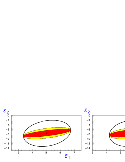
Figure 3: 70% confidence level contour plots for fits to $\epsilon$’s in units of $10^{-3}$. The outer contour is for a fit with the current error, $\Delta M_{\mathrm{W}}=\pm 160\;{\rm MeV}$, whereas the inner contours are for $\Delta M_{\mathrm{W}}=\pm 50\;{\rm MeV}$ and $\Delta M_{\mathrm{W}}=\pm 25\;{\rm MeV}$ respectively.

Numerically, the projected data give a precision

$$\Delta\epsilon_{1}=\pm 1.1\times 10^{-3}\hskip 42.67912pt\Delta\epsilon_{3}=\pm 1.0\times 10^{-3}\,.$$ (3)

For $\Delta M_{\mathrm{W}}=160\;{\rm MeV}$, the error $\Delta\epsilon_{2}=\pm 3.7\times 10^{-3}$ is obtained, whereas for the projected errors on $M_{\mathrm{W}}$ one obtains

$$\Delta\epsilon_{2}=\pm 1.0\,(\pm 1.6)\,\times 10^{-3}\hskip 28.45274pt\mbox{for}\hskip 17.07182pt\Delta M_{\mathrm{W}}=25\,(50)\;{\rm MeV}\,.$$ (4)

The smaller the volume in $\epsilon$ space allowed by the precision electroweak measurements, the greater the constraint on physics beyond the Standard Model.

The MSSM is arguably the most promising new-physics candidate. It is therefore especially important to consider the MSSM prediction for $M_{\mathrm{W}}$. Figure 4 [15] shows $M_{\mathrm{W}}$ as a function of $M_{\mathrm{t}}$ in the SM (solid lines) and in the MSSM (dashed lines). In each case the prediction is a band of values, corresponding to a variation of the model parameters (dominantly $M_{\mathrm{H}}$ in the SM case, with $90\;{\rm GeV}<\mbox{$M_{\mathrm{H}}$}<1000\;{\rm GeV}$ chosen here) consistent with current measurements and limits. An additional constraint of ‘no SUSY particles at LEP2’ is imposed in the MSSM calculation.

Figure 4: Predictions for $M_{\mathrm{W}}$ as a function of $M_{\mathrm{t}}$ in the SM (solid lines) and in the MSSM (dashed lines), from Ref. [15]. In each case the prediction is a band of values, corresponding to a variation of the model parameters consistent with current measurements and limits. An additional constraint of ‘no SUSY particles at LEP2’ is imposed in the MSSM calculation.

1.5 Methods for measuring $M_{\mathrm{W}}$

Precise measurements of $M_{\mathrm{W}}$ can in principle be obtained using the enhanced statistical power of the rapidly varying total cross-section at threshold, the sharp (Breit-Wigner) peaking behaviour of the invariant-mass distribution of the W^± decay products and the sharp end-point spectrum of the lepton energy in W^± decay. One can obtain a rough idea of the relative power of these methods by estimating their statistical precision assuming 100% efficiency, perfect detectors and no background. More complete discussions are given in Sections 2 and 3.

• Threshold cross-section measurement of the process $\mbox{$\mathrm{e^{+}e^{-}}$}\rightarrow\mbox{$\mathrm{W^{+}W^{-}}$}$. The statistical power of this method, assuming 100% signal efficiency and no background, is

  $$\Delta M_{\mathrm{W}}\geq 91\;{\rm MeV}\sqrt{{100\;{\rm pb}^{-1}\over{\cal L}}}\,,$$ (5)

  where the minimum value is attained at $\sqrt{s}\simeq 161\;{\rm GeV}$. Here ${\cal L}$ denotes the total integrated luminosity.

• Direct reconstruction methods, which reconstruct the Breit-Wigner resonant shape from the W^± final states using kinematic fitting techniques to improve the mass resolution. The statistical power of this method, again assuming 100% efficiency, perfect detector resolution and no background, can be estimated as

  $$\Delta M_{\mathrm{W}}\sim\frac{\Gamma_{\rm W}}{\sqrt{N}}\approx 50\;{\rm MeV}\sqrt{{100\;{\rm pb}^{-1}\over{\cal L}}}\,,$$ (6)

  approximately independent of the collider energy. This order of magnitude estimate is confirmed by more detailed studies, see below.

• Determination of $M_{\mathrm{W}}$ from the lepton end-point energy. The end-points of the lepton spectrum in $\mbox{$\mathrm{W^{+}W^{-}}$}\rightarrow\mbox{$\mathrm{q\overline{q}}$}l\nu$ depend quite sensitively on the W mass. For on-shell W bosons at leading order:

  $$E_{-}\leq E_{l}\leq E_{+}\;,\qquad E_{\pm}={\sqrt{s}\over 4}\;\left(1\pm\sqrt{1-4M_{\mathrm{W}}^{2}/s}\right)\;.$$ (7)

  In this case the statistical error on $M_{\mathrm{W}}$ is determined by the statistical error on the measurement of the lepton end-point energy,

  $$\Delta M_{\mathrm{W}}=\frac{\sqrt{s-4M_{\mathrm{W}}^{2}}}{M_{\mathrm{W}}}\;\Delta E_{\pm}\,.$$ (8)

  In practice, however, the end-points of the distribution are considerably smeared by finite width effects and by initial state radiation, and only a fraction of events close to the end-points are sensitive to $M_{\mathrm{W}}$. This significantly weakens the statistical power of this method from what the naive estimate (8) would predict.

The detailed studies described in the following sections show that the errors which can realistically be achieved in practice are somewhat larger than the above estimates for Methods A and B. The statistical precisions of the two methods are in fact more comparable (for the same integrated luminosity) than the factor 2 difference suggested by the naive estimates (5) and (6). The overall statistical error for Method C has been estimated at ${\cal O}(300\;{\rm MeV})$ [1] for ${\cal L}=500\;{\rm pb}^{-1}$ , significantly larger than that of the other two methods. It will not therefore be considered further here, although it is still a valid measurement for cross-checking the other results.

It is envisaged that most of the LEP2 data will be collected at energies well above threshold, and so the statistically most precise determination of $M_{\mathrm{W}}$ will come from Method B. However with a relatively modest amount of luminosity spent at the $\mathrm{W^{+}W^{-}}$ threshold (for example $50\;{\rm pb}^{-1}$ per experiment), Method A can provide a statistical error of order $100\;{\rm MeV}$, not significantly worse than Method B and with very different systematics. The two methods can therefore be regarded as complementary tools, and both should be used to provide an internal cross-check on the measurement of the W mass at LEP2. This constitutes the main motivation for spending some luminosity in the threshold region.

The threshold cross-section method is also of interest because it appears to fit very well into the expected schedule for LEP2 operation in 1996. It is anticipated that the maximum beam energy at LEP2 will increase in steps, with the progressive installation of more superconducting RF cavities, in such a way that a centre-of-mass energy of 161 GeV will indeed be achievable during the first running period of 1996. This would then be the ideal time to perform such a threshold measurement. The achievable statistical error on $M_{\mathrm{W}}$ depends of course critically on the available luminosity at the threshold energy. In Section 2 we present quantitative estimates based on integrated luminosities of 25, 50 and 100 pb^-1 per experiment.

1.6 Theoretical input information

1.6.1 Cross-sections for the $\mathrm{W^{+}W^{-}}$ signal and backgrounds

Methods (A) and (B) for measuring $M_{\mathrm{W}}$ described above require rather different theoretical input. The threshold method relies on the comparison of an absolute cross-section measurement with a theoretical calculation which has $M_{\mathrm{W}}$ as a free parameter. The smallness of the cross-section near threshold is compensated by the enhanced sensitivity to $M_{\mathrm{W}}$ in this region. In contrast, the direct reconstruction method makes use of the large $\mathrm{W^{+}W^{-}}$ statistics at the higher LEP2 energies, $\sqrt{s}{\ \lower 2.58334pt\hbox{$\buildrel>\over{\sim}$}\ }175$ GeV. Here the more important issue is the accurate modeling of the W^± line-shape, i.e. the distribution in the invariant mass of the W^± decay products.

In this section we describe some of the important features of the theoretical cross-sections which are relevant for the $M_{\mathrm{W}}$ measurements. A more complete discussion can be found in the contribution of the WW and Event Generators Working Group to this Report [18].

We begin by writing the cross-section for $\mbox{$\mathrm{e^{+}e^{-}}$}\rightarrow 4\mathrm{f}\;(+\gamma,\mathrm{g},\ldots)$, schematically, as

$$\sigma = \sigma_{\rm WW}\;+\;\sigma_{\rm bkd}\;,$$

$$\sigma_{\rm WW} = \sigma_{0}^{\rm WW}\;(1+\delta_{\rm EW}+\delta_{\rm QCD})\;,$$ (9)

We note that this decomposition of the cross-section into ‘signal’ and ‘background’ contributions is practical rather than theoretically rigorous, since neither contribution is separately exactly gauge invariant nor experimentally distinguishable in general. The various terms in (9) correspond to

• $\sigma_{0}^{\rm WW}$: the Born contribution from the 3 ‘CC03’ leading-order diagrams for $\mbox{$\mathrm{e^{+}e^{-}}$}\rightarrow\mbox{$\mathrm{W^{+}W^{-}}$}$ involving $t$-channel $\nu$ exchange and $s$-channel $\gamma$ and Z⁰ exchange, calculated using off-shell W propagators.

• $\delta_{\rm EW}$: higher-order electroweak radiative corrections, including loop corrections, real photon emission, etc.

• $\delta_{\rm QCD}$: higher-order QCD corrections to $\mathrm{W^{+}W^{-}}$ final states containing $\mathrm{q\overline{q}}$ pairs. For the threshold measurement, where in principle only the total cross-section is of primary interest, the effect of these is to generate small corrections to the hadronic branching ratios which are entirely straightforward to calculate and take into account. More generally, such QCD corrections can lead to additional jets in the final state, e.g. $\mbox{$\mathrm{W^{+}W^{-}}$}\rightarrow\mbox{$\mathrm{q\overline{q}}$}\mbox{$\mathrm{q\overline{q}}$}\mathrm{g}$ from one hard gluon emission. This affects the direct reconstruction method, insofar as the kinematic fits to reconstruct $M_{\mathrm{W}}$ assume a four-jet final state, and both methods insofar as cuts have to be imposed in order to suppress the QCD background (see Sections 2,3 below). Perturbative QCD corrections, real gluon emission to $O(\alpha_{s}^{2})$ and real plus virtual emission to $O(\alpha_{s})$, have been recently discussed in Refs. [19, 20] respectively, together with their impact on the measurement of $M_{\mathrm{W}}$.

• $\sigma_{\rm bkd}$: ‘background’ contributions, for example from non-resonant diagrams (e.g. $e^{+}e^{-}\rightarrow\mu^{+}\nu_{\mu}\mathrm{W}^{-}$) and QCD contributions $\mbox{$\mathrm{e^{+}e^{-}}$}\rightarrow\mbox{$\mathrm{q\overline{q}}$}\mathrm{gg}(\gamma),\;\mbox{$\mathrm{q\overline{q}}$}\mbox{$\mathrm{q\overline{q}}$}(\gamma)$ to the four-jet final state. All of the important backgrounds have been calculated, see Table 6 below. At threshold, the QCD four-jet background is particularly large in comparison to the signal.

In what follows we consider (i) and (ii) in some detail. Background contributions and how to suppress them are considered in later sections.

1.6.2 The $\mathrm{W^{+}W^{-}}$ off-shell cross-section

The leading-order cross-section for off-shell $\mathrm{W^{+}W^{-}}$ production was first presented in Ref. [21]:

$$\sigma(s)=\int_{0}^{s}ds_{1}\int_{0}^{(\sqrt{s}-\sqrt{s_{1}})^{2}}ds_{2}\;\rho(s_{1})\rho(s_{2})\;\sigma_{0}(s,s_{1},s_{2})\;,$$ (10)

where

$$\rho(s)={1\over\pi}{\Gamma_{\mathrm{W}}\over M_{\mathrm{W}}}\;{s\over(s-M_{\mathrm{W}}^{2})^{2}+s^{2}\Gamma_{\mathrm{W}}^{2}/M_{\mathrm{W}}^{2}}\;.$$ (11)

The cross-section $\sigma_{0}$ can be written in terms of the $\nu$, $\gamma$ and Z exchange contributions and their interferences:

$$\sigma_{0}(s,s_{1},s_{2})={g^{4}\over 256\pi s^{2}s_{1}s_{2}}\;\left[a_{\gamma\gamma}+a_{ZZ}+a_{\gamma Z}+a_{\nu\nu}+a_{\nu Z}+a_{\nu\gamma}\right]\;,$$ (12)

where $g^{4}=e^{4}/\sin^{4}\theta_{W}$. Explicit expressions for the various contributions can be found in Ref. [21] for example. The stable (on-shell) $\mathrm{W^{+}W^{-}}$ cross-section is simply

$$\sigma^{\rm on}(s)=\sigma_{0}(s,M_{\mathrm{W}}^{2},M_{\mathrm{W}}^{2})\;.$$ (13)

A theoretical ansatz of this kind will be the basis of any experimental determination of the mass and width of the W boson. The reason for this is the large effect of the virtuality of the W bosons produced around the nominal threshold. An immediate conclusion from Eq. (10) may be drawn: the W mass influences the cross sections exclusively through the off-shell $W$ propagators; all the other parts are independent of $M_{\mathrm{W}}$ and $\Gamma_{\mathrm{W}}$ (neglecting for the moment the relatively minor dependence due to radiative corrections). It will be an important factor in the discussion which follows that near threshold the (unpolarized) cross-section is completely dominated by the $t$-channel neutrino exchange diagram. This leads to an $S$-wave threshold behaviour $\sigma_{t}\sim\beta$, whereas the $s$-channel vector boson exchange diagrams give the characteristic $P$-wave behaviour $\sigma_{s}\sim\beta^{3}$.

By tradition (for example at LEP1 with the Z boson), the virtual W propagator in Eq. (11) uses an $s$-dependent width,

$$\Gamma_{\mathrm{W}}(s)={s\over M_{\mathrm{W}}^{2}}\;\Gamma_{\mathrm{W}}\;,$$ (14)

where $\Gamma_{\mathrm{W}}\equiv\Gamma_{\mathrm{W}}(M_{\mathrm{W}}^{2})$. Another choice, equally well justified from a theoretical point of view, would be to use a constant width in the W propagator (for a discussion see Ref. [22]):

$${\overline{\rho}}=\frac{1}{\pi}\frac{{\overline{M}}_{\mathrm{W}}{\overline{\Gamma}}_{\mathrm{W}}}{\left(s-{\overline{M}}_{\mathrm{W}}^{2}\right)^{2}+{\overline{M}}_{\mathrm{W}}^{2}{\overline{\Gamma}}_{\mathrm{W}}^{2}}\;.$$ (15)

The numerical values of the width and mass in the two expressions are related [23]:

$${\overline{M}}_{\mathrm{W}} = M_{\mathrm{W}}-\frac{1}{2}\frac{\Gamma_{\mathrm{W}}^{2}}{M_{\mathrm{W}}}=M_{\mathrm{W}}-26.9\;{\rm MeV}\;,$$ (16)

$${\overline{\Gamma}}_{\mathrm{W}} = \Gamma_{\mathrm{W}}-\frac{1}{2}\frac{\Gamma_{\mathrm{W}}^{3}}{M_{\mathrm{W}}^{2}}=\Gamma_{\mathrm{W}}-0.7\;{\rm MeV}\;.$$ (17)

These relations may be derived from the following identity: $(s-{\overline{M}}_{\mathrm{W}}^{2}+i{\overline{M}}_{\mathrm{W}}{\overline{\Gamma}}_{\mathrm{W}})=(s-M_{\mathrm{W}}^{2}+is\Gamma_{\mathrm{W}}/M_{\mathrm{W}})/(1+i\Gamma_{\mathrm{W}}/M_{\mathrm{W}})$. Numerically, the consequences are below the anticipated experimental accuracy.

1.6.3 Higher-order electroweak corrections

The complete set of $O(\alpha)$ next-to-leading order corrections to $\mathrm{W^{+}W^{-}}$ production has been calculated by several groups [24, 25], for the on-shell case only, see for example Refs. [26, 18] and references therein. There has been some progress with the off-shell (i.e. four fermion production) corrections but the calculation is not yet complete. However using the on-shell calculations as a guide, it is already possible to predict some of the largest effects. For example, it has been shown that close to threshold the dominant contribution comes from the Coulomb correction, i.e. the long-range electromagnetic interaction between almost stationary heavy particles. Also important is the emission of photons collinear with the initial state e^± (‘initial state radiation’) which gives rise to logarithmic corrections $\sim\alpha\ln(s/m_{e}^{2})$. These leading logarithms can be resummed to all orders, and incorporated for example using a ‘structure function’ formalism. In this case, the generalization from on-shell to off-shell $W$’s appears to be straightforward. For the Coulomb corrections, however, one has to be much more careful, since in this case the inclusion of the finite $W$ decay width has a dramatic effect. Finally, one can incorporate certain important higher-order fermion and boson loop corrections by a judicious choice of electroweak coupling constant. Each of these effects will be discussed in turn below.

In summary, certain $O(\alpha)$ corrections are already known to be large because their coefficients involve large factors like $\ln(s/m_{e}^{2})$, $\sqrt{M_{\mathrm{W}}/\Gamma_{\mathrm{W}}}$, $M_{\mathrm{t}}^{2}/M_{\mathrm{W}}^{2}$, etc. Once these are taken into account, one can expect that the remaining corrections are no larger than ${\cal O}(\alpha)$. When estimating the theoretical systematic uncertainty on the W mass in Section 2 below, we shall therefore assume a conservative overall uncertainty on the cross-section of $\pm 2\%$ from the as yet uncalculated $O(\alpha)$ and higher-order corrections.

1.6.4 Coulomb corrections

The Coulomb corrections for on-shell and off-shell $\mathrm{W^{+}W^{-}}$ production have been discussed in detail in Refs. [27, 28, 29], where a complete set of references to earlier studies can also be found.

The result for on-shell $\mathrm{W^{+}W^{-}}$ production is well-known [30] — the $O(\alpha)$ correction diverges as $\alpha\pi/v_{0}$ as the relative velocity $v_{0}=2[1-4M_{\mathrm{W}}^{2}/s]^{1/2}$ of the $W$ bosons approaches zero at threshold. Note that $\sigma_{0}\sim v_{0}$ near threshold and so the Coulomb-corrected cross-section is formally non-vanishing when $\sqrt{s}=2M_{\mathrm{W}}$.

For unstable $\mathrm{W^{+}W^{-}}$ production the finite decay width $\Gamma_{\mathrm{W}}$ screens the Coulomb singularity [27], so that very close to threshold the perturbative expansion in $\alpha\pi/v_{0}$ is effectively replaced by an expansion in $\alpha\pi\sqrt{M_{\mathrm{W}}/\Gamma_{\mathrm{W}}}$ [28]. In the calculations which follow we use the expressions for the $O(\alpha)$ correction given in Ref. [28]. The net effect is a correction which reaches a maximum of approximately $+6\%$ in the threshold region. Although this does not appear to be large, we will see below that it changes the threshold cross-section by an amount equivalent to a shift in $M_{\mathrm{W}}$ of order $100$ MeV. In Ref. [28] the $O(\alpha)$ result is generalized to all orders. However the contributions from second order and above change the cross-section by $\ll 1\%$ in the threshold region [31] (see also [29]) and can therefore be safely neglected.

Note also that the Coulomb correction to the off-shell $\mathrm{W^{+}W^{-}}$ cross-section

$$\sigma(s)=\int_{0}^{s}ds_{1}\int_{0}^{(\sqrt{s}-\sqrt{s_{1}})^{2}}ds_{2}\;\rho(s_{1})\rho(s_{2})\;\sigma_{0}(s,s_{1},s_{2})[1+\delta_{C}(s,s_{1},s_{2})]$$ (18)

provides an example of a (QED) interconnection effect between the two W bosons: the exchange of a soft photon distorts the line shape ($d\sigma/d\sqrt{s_{1}}$) of the W^± and therefore, at least in principle, affects the direct reconstruction method [32, 33, 34]. In Ref. [32], for example, it is shown that the Coulomb interaction between the W bosons causes a downwards shift in the average reconstructed mass of $O(\pi\alpha\Gamma_{\mathrm{W}})\sim O(20\;{\rm MeV})$. Selecting events close to the Breit-Wigner peak reduces the effect somewhat. However the calculations are not yet complete, in that QED interactions between the decay products of the two W bosons are not yet fully included.

1.6.5 Initial state radiation

Another important class of electroweak radiative corrections comes from the emission of photons from the incoming e⁺ and e^-. In particular, the emission of virtual and soft real photons with energy $E<\omega$ gives rise to doubly logarithmic contributions $\sim\alpha\ln(s/m_{e}^{2})\ln(s/\omega^{2})$ at each order in perturbation theory. The infra-red ($\ln\omega$) logarithms cancel when hard photon contributions are added, and the remaining collinear ($\ln(s/m_{e}^{2})$) logarithms can be resummed and incorporated in the cross-section using a ‘flux function’ or a ‘structure function’ [35] (see also Refs. [36, 37, 38, 39, 18]).

The ISR corrected cross section in the flux function (FF) approach is

$$\frac{d\sigma_{\mathrm{ISR}}(s)}{ds_{1}ds_{2}} = \int\limits_{s_{\min}}^{s}\frac{ds^{\prime}}{s}\Biggl{\{}F(x,s)\Bigl{[}\sigma_{\tt CCn}(s^{\prime},s_{1},s_{2})+~{}\delta_{C}\,\sigma_{\tt CC3}(s^{\prime},s_{1},s_{2})\Bigr{]}+~{}\sigma_{\mathrm{ISR}}^{\mathrm{non-univ}}\Biggr{\}},$$ (19)

where $x=1-s^{\prime}/s$ and

$$F(x,s) = tx^{t-1}(1+S)+H(s^{\prime},s)\;,$$ (20)

with

$$t = \frac{2\alpha}{\pi}\left[\ln\left(\frac{s}{m_{e}^{2}}\right)-1\right]\;.$$ (21)

The ${\cal S}$ term comes from soft and virtual photon emission, the ${\cal H}$ term comes from hard photon emission, $\delta_{C}$ contains the Coulomb correction (18), $\sigma_{\tt CC3}$ is the doubly resonating Born cross section, and $\sigma_{\tt CCn}$ the background contributions. Explicit expressions can be found in the above references. The additional term $\sigma_{\mathrm{ISR}}^{\mathrm{non-univ}}$ is discussed in Refs. [38] and [18]. The invariant mass lost to photon radiation may be calculated as

$$\langle m_{\gamma}\rangle = \frac{1}{\sigma}\int ds_{1}ds_{2}\,\int\frac{ds^{\prime}}{s}\frac{\sqrt{s}}{2}\left(1-\frac{s^{\prime}}{s}\right)\frac{d\sigma}{ds_{1}ds_{2}ds^{\prime}},$$ (22)

where $d\sigma/ds_{1}ds_{2}ds^{\prime}$ is the contents of the curly brackets in Eq. (19).

Alternatively, the structure function (SF) approach may be used:

$$\frac{d\sigma_{\mathrm{QED}}(s)}{ds_{1}ds_{2}} = \int\limits_{x_{1}^{\min}}^{1}dx_{1}\int\limits_{x_{2}^{\min}}^{1}dx_{2}\,D(x_{1},s)D(x_{2},s)\Biggl{\{}\sigma_{\tt CCn}(x_{1}x_{2}s,s_{1},s_{2})+~{}\delta_{C}~{}\sigma_{\tt CC3}\Biggr{\}}\;,$$ (23)

where

$$D(x,s) = \frac{t}{2}(1-x)^{t/2-1}(1+{\overline{S}})+{\overline{H}}(x,s)\;.$$ (24)

Here, the invariant mass loss is

$$\langle m_{\gamma}\rangle = \frac{1}{\sigma}\int ds_{1}ds_{2}\int dx_{1}dx_{2}\,D(x_{1},s)D(x_{2},s)\frac{\sqrt{s}}{2}(1-x_{1}x_{2})\frac{d\sigma(x_{1}x_{2}s,s_{1},s_{2})}{ds_{1}ds_{2}dx_{1}dx_{2}}.$$ (25)

In addition, the radiative energy loss may be determined,

$$\langle E_{\gamma}\rangle = \frac{1}{\sigma}\int ds_{1}ds_{2}\int dx_{1}dx_{2}\,D(x_{1},s)D(x_{2},s)\frac{\sqrt{s}}{2}(2-x_{1}-x_{2})\frac{d\sigma}{ds_{1}ds_{2}dx_{1}dx_{2}}\;.$$

Initial state radiation affects the W mass measurement in two ways. Close to threshold the cross-section is smeared out, thus reducing the sensitivity to $M_{\mathrm{W}}$ (see Fig. 5 below). For the direct reconstruction method, the relatively large average energy carried away by the radiated photons leads to a large positive mass-shift if it is not taken into account in the rescaling of the final-state momenta to the beam energy (see Section 3 below). By rescaling to the nominal beam energy we obtain for the mass-shift $\Delta M_{\mathrm{W}}$ $=$  $\langle E_{\gamma}\rangle M_{\mathrm{W}}/\sqrt{s}$. Note however that a fit to the mass distribution gives more weight to the peak, and therefore in practice the effective value of $\langle E_{\gamma}\rangle$ or $\langle m_{\gamma}\rangle$ is less than that given by Eqs. (22,25,LABEL:eq:26) (see Section 3.4). Table 3 shows the influence of the various cross-section contributions on the average energy and invariant mass losses. The invariant mass loss may be calculated both in the SF and FF approaches. A comparison shows that the predictions in both schemes differ only slightly, which allows us to use the numerically faster FF approach for the numerical estimates. At the lower LEP2 collider energies, the energy and invariant mass losses are nearly equal, while at higher energies their difference is non-negligible. Note also that the inclusion of the non-universal ISR corrections and background terms is of minor influence. The latter has been studied only for CC11 processes; for reactions of the CC20 type the background is larger and the numerical estimates are not yet available. The Coulomb correction is numerically important and cannot be neglected [29]. The dependence of the predictions on the details of the treatment of QED is discussed in detail in Ref. [18] and will not be repeated here.

	$\sqrt{s}$ (GeV)	175	192	205
SF, CC3	$\sigma$ (pb)	13.182	16.488	17.077
	$\langle E_{\gamma}\rangle$	1115	2280	3202
	$\langle m_{\gamma}\rangle$	1112	2271	3185
	$\langle E_{\gamma}\rangle$–$\langle m_{\gamma}\rangle$	3	9	17
change to FF	$\Delta\langle m_{\gamma}\rangle$	0.5	–0.8	–4.2
add $\delta_{C}$	$\Delta\langle m_{\gamma}\rangle$	11.8	16.3	20.8
add $\sigma_{\rm{ISR}}^{non-univ}$	$\Delta\langle m_{\gamma}\rangle$	0.2	0.3	0.3
add $\sigma_{\tt CCn}$	$\Delta\langle m_{\gamma}\rangle$	$\leq$0.1	0.2	0.5

Table 3: Influence of different cross-section treatments on the average energy loss $\langle E_{\gamma}\rangle$ and invariant mass loss $\langle m_{\gamma}\rangle$ in MeV.

parameter	value
$M_{\mathrm{Z}}$	91.1888
$M_{\mathrm{W}}$	80.23
$\Gamma_{\mathrm{Z}}$	2.4974
$\Gamma_{\mathrm{W}}$	2.078
$\alpha^{-1}$	137.0359895
$G_{\mu}$	$1.16639\times 10^{-5}$ GeV-2
$\sin^{2}\theta_{W}\equiv\sin^{2}\theta_{W}^{(\ell)\rm eff}$	0.2320
$m_{e}$	$5.1099906\times 10^{-4}$
$(\hbar c)^{2}$	$3.8937966\times 10^{8}$ pb GeV2

Table 4: Parameter values used in the numerical calculations in Table 5 and Fig. 5. Masses and widths are given in GeV.

1.6.6 Improved Born approximation

In the Standard Model, three parameters are sufficient to parametrise the electroweak interactions, and the conventional choice is $\{\alpha,G_{\mu},M_{\mathrm{Z}}\}$ since these are the three which are measured most accurately. In this case the value of $M_{\mathrm{W}}$ is a prediction of the model. Radiative corrections to the expression for $M_{\mathrm{W}}$ in terms of these parameters introduce non-trivial dependences on $M_{\mathrm{t}}$ and $M_{\mathrm{H}}$, and so a measurement of $M_{\mathrm{W}}$ provides a constraint on these masses. However the choice $\{\alpha,G_{\mu},M_{\mathrm{Z}}\}$ does not appear to be well suited to $\mathrm{W^{+}W^{-}}$ production. The reason is that a variation of the parameter $M_{\mathrm{W}}$, which appears explicitly in the phase space and in the matrix element, has to be accompanied by an adjustment of the charged and neutral weak couplings. Beyond leading order this is a complicated procedure.

It has been argued [40] that a more appropriate choice of parameters for LEP2 is the set $\{M_{\mathrm{W}},G_{\mu},M_{\mathrm{Z}}\}$ (the so-called $G_{\mu}$–scheme), since in this case the quantity of prime interest is one of the parameters of the model. Using the tree-level relation

$$g^{2}=e^{2}/\sin^{2}\theta_{W}=4\sqrt{2}G_{\mu}M_{\mathrm{W}}^{2}$$ (27)

we see that the dominant $t$-channel neutrino exchange amplitude, and hence the corresponding contribution to the cross-section, depends only on the parameters $M_{\mathrm{W}}$ and $G_{\mu}$. It has also been shown [40] that in the $G_{\mu}$–scheme there are no large next-to-leading order contributions to the cross-section which depend on $M_{\mathrm{t}}$, either quadratically or logarithmically. One can go further and choose the couplings which appear in the other terms in the Born cross-section such that all large corrections at next-to-leading order are absorbed, see for example Ref. [41]. However for the threshold cross-section, which is dominated by the $t$-channel exchange amplitude, one can simply use combinations of $e^{2}$ and $g^{2}$ defined by Eq. (27) for the neutral and charged weak couplings which appear in the Born cross-section, Eq. (12).

In summary, the most model-independent approach when defining the parameters for computing the $\mbox{$\mathrm{e^{+}e^{-}}$}\rightarrow\mbox{$\mathrm{W^{+}W^{-}}$}$ cross-section appears to be the $G_{\mu}$–scheme, in which $M_{\mathrm{W}}$ appears explicitly as a parameter of the model. Although this makes a non-negligible difference when calculating the Born cross-section, compared to using $\alpha$ and $\sin^{2}\theta_{W}$ to define the weak couplings (see Table 5 below), a full next-to-leading-order calculation will remove much of this scheme dependence [40].

$\sigma_{WW}$	$\sqrt{s}=161$ GeV	$\sqrt{s}=175$ GeV
$\sigma_{0}$ (on-shell, $\alpha$)	3.813	15.092
$\sigma_{0}$ (on-shell, $G_{\mu}$)	4.402	17.425
$\sigma_{0}$ (off-shell with $\Gamma_{\mathrm{W}}(M_{\mathrm{W}}^{2})$, $G_{\mu}$)	4.747	15.873
$\sigma_{0}$ (off-shell with $\Gamma_{\mathrm{W}}(s)$, $G_{\mu}$)	4.823	15.882
$\ldots\ +$ $O(\alpha)$ Coulomb	5.122	16.311
$\ldots\ +$ $O(\alpha)$ Coulomb $+$ ISR	3.666	13.620

Table 5: Decomposition of the theoretical $e^{+}e^{-}\rightarrow W^{+}W^{-}$ cross-section (in picobarns) as defined and discussed in the text, at two LEP2 collider energies.

1.6.7 Numerical evaluation of the cross-section

Figure 5 shows the $\mbox{$\mathrm{e^{+}e^{-}}$}\rightarrow\mbox{$\mathrm{W^{+}W^{-}}$}$ cross-section at LEP2 energies. The different curves correspond to the sequential inclusion of the different effects discussed above. The parameters used in the calculation are listed in Table 4. Note that both the initial state radiation and the finite width smear the sharp threshold behaviour at $\sqrt{s}=2M_{\mathrm{W}}$ of the on-shell cross-section.

Figure 5: The cross-section for $\mbox{$\mathrm{e^{+}e^{-}}$}\rightarrow W^{+}W^{-}$ in various approximations: (i) Born (on-shell) cross-section, (ii) Born (off-shell) cross-section, (iii) with first order Coulomb corrections, and (iv) with initial state radiation. The parameter values are listed in Table 4.

The different contributions are quantified in Table 5, which gives the values of the cross-section in different approximations just above threshold ($\sqrt{s}=161$ GeV) and at the standard LEP2 energy of $\sqrt{s}=175$ GeV. At threshold we see that the effects of initial state radiation and the finite W width are large and comparable in magnitude. For the threshold method, the primary interest is the dependence of the cross-section on $M_{\mathrm{W}}$.

Reaction	Cross-section (pb)
	at 161 GeV	at 175 GeV	at 192 GeV
$\mbox{$\mathrm{e^{+}e^{-}}$}\rightarrow\mbox{$\mathrm{W^{+}W^{-}}$}\rightarrow\mathrm{all}$	3.64	13.77	17.10
$\mbox{$\mathrm{e^{+}e^{-}}$}\rightarrow\mbox{\mbox{$\mathrm{W^{+}W^{-}}$}$\rightarrow$\mbox{$\mathrm{q\overline{q}}$}\mbox{$\mathrm{q\overline{q}}$}}$	1.67	6.30	7.85
$\mbox{$\mathrm{e^{+}e^{-}}$}\rightarrow\mbox{\mbox{$\mathrm{W^{+}W^{-}}$}$\rightarrow$\mbox{$\mathrm{q\overline{q}}$}\mbox{$l\nu$}}$	1.59	6.02	7.46
$\mbox{$\mathrm{e^{+}e^{-}}$}\rightarrow\mbox{\mbox{$\mathrm{W^{+}W^{-}}$}$\rightarrow$\mbox{$l\nu$}\mbox{$l\nu$}}$	0.38	1.44	1.79
$\mbox{$\mathrm{e^{+}e^{-}}$}\rightarrow\mathrm{Z}/\gamma\rightarrow\mathrm{all}$	221.	172.	135.
$\mbox{$\mathrm{e^{+}e^{-}}$}\rightarrow\mathrm{Z}/\gamma\rightarrow\mbox{$\mathrm{q\overline{q}}$}$	151.	116.	91.
$\mbox{$\mathrm{e^{+}e^{-}}$}\rightarrow\mathrm{Z}/\gamma\rightarrow l^{+}l^{-},\nu\overline{\nu}$	70.	56.	44.
$\mbox{$\mathrm{e^{+}e^{-}}$}\rightarrow(\mathrm{Z}/\gamma)(\mathrm{Z}/\gamma)\rightarrow\mathrm{all}$	0.46	0.44	1.12
$\mbox{$\mathrm{e^{+}e^{-}}$}\rightarrow\mathrm{Zee}\rightarrow\mathrm{all}$	2.53	2.70	2.85
$\mbox{$\mathrm{e^{+}e^{-}}$}\rightarrow\mathrm{We}\nu\rightarrow\mathrm{all}$	0.37	0.51	0.72
$\mbox{$\mathrm{e^{+}e^{-}}$}\rightarrow\mbox{$\mathrm{e^{+}e^{-}}$}$, $|\cos\theta|<0.95$	351.	297.	247.

Table 6: Cross-sections (in picobarns) for signal and background channels as given by PYTHIA. $\mathrm{W^{+}W^{-}}$, $(\mathrm{Z}/\gamma)(\mathrm{Z}/\gamma)$, $\mathrm{We}\nu$ and $\mathrm{Zee}$ refer to four-fermion production with intermediate formation of either one or two vector bosons; in the case of Z pair production, the generator includes the photon contribution. The process $\mathrm{Z}/\gamma\rightarrow\mathrm{all}$ refers to the production of a fermion pair via a Z boson or photon. All interactions include initial state radiation, and therefore may contain additional photons in the final state. The final row lists cross-sections generated for the Bhabha scattering process (including t-channel exchange) using the BABAMC program.

This will be quantified in Section 2 below. For both methods, the size of the background cross-sections is important. For completeness, therefore, we list in Table 6 some relevant cross-section values obtained using the PYTHIA Monte Carlo. This includes finite-width effects, initial state radiation and Coulomb corrections. Notice that the values for $\sigma_{WW}$ agree to within about 1% accuracy with those given in the last row of Table 5.

2 Measurement of $M_{\mathrm{W}}$ from the $\mathrm{W^{+}W^{-}}$ Threshold Cross-Section

As discussed in Section 1.5, one can exploit the rapid increase of the $\mathrm{W^{+}W^{-}}$ production cross-section at $\sqrt{s}\sim 2M_{\mathrm{W}}$ to measure the W mass. In the following, we briefly discuss the basic features of this method, suggest an optimal collider strategy for data-taking, and estimate the statistical and systematic errors. The intrinsic statistical limit to the resolution on $M_{\mathrm{W}}$ is shown to be energy-dependent: in particular, arguments are presented in favour of a single cross-section measurement at a fixed energy $\sqrt{s}\sim 161\;\mathrm{GeV}$.

2.1 Collider strategy

The cross-section for $\mathrm{W^{+}W^{-}}$ production increases very rapidly near the nominal kinematic threshold $\sqrt{s}=2M_{\mathrm{W}}$, although the finite W width and ISR smear out the abrupt rise of the Born on-shell cross-section. This means that for a given $\sqrt{s}$ near threshold, the value of the cross-section is very sensitive to $M_{\mathrm{W}}$. This is illustrated in Fig. 6, where the $\mathrm{W^{+}W^{-}}$ excitation curve is plotted for various values of the W mass. The calculation is the same as that discussed in Section 1.6, and includes finite W width effects, ISR and QED Coulomb corrections. A measurement of the cross-section in this region therefore directly yields a measurement of $M_{\mathrm{W}}$.

Figure 6: The cross-section for $\mathrm{W^{+}W^{-}}$ production as a function of $\sqrt{s}$  in the threshold region, for various values of $M_{\mathrm{W}}$. Finite-width effects, the QED Coulomb correction and Initial State Radiation are included.

For an integrated luminosity $\cal{L}$ and an overall signal efficiency $\epsilon_{WW}=\sum_{i}\epsilon_{i}\mathrm{BR}_{i}$ (where the sum extends over the various channels selected, with branching ratios BR_i and efficiencies $\epsilon_{i}$), the error on the $\mathrm{W^{+}W^{-}}$ cross-section due to signal statistics is given by

$$\Delta\sigma_{WW}={\sigma_{WW}\over\sqrt{N}}={\sqrt{\sigma_{WW}}\over\sqrt{\epsilon_{WW}{\cal L}}},$$ (28)

where $N=\epsilon_{WW}\sigma_{WW}{\cal L}$ is the number of selected signal events. The corresponding error on the W mass is

$$\Delta M_{\mathrm{W}}=\sqrt{\sigma_{WW}}\left|\frac{dM_{\mathrm{W}}}{d\sigma_{WW}}\right|\frac{1}{\sqrt{\epsilon_{WW}\cal{L}}}.$$ (29)

The sensitivity factor $\sqrt{\sigma_{WW}}|{dM_{\mathrm{W}}}/d\sigma_{WW}|$ is plotted in Fig. 7 as a function of $\sqrt{s}-2M_{\mathrm{W}}$. There is a minimum at

$$(\sqrt{s})^{\,\mathrm{opt}}\simeq 2M_{\mathrm{W}}+0.5\;\mathrm{GeV},$$ (30)

corresponding to a minimum value of approximately $0.91\mathrm{\;{\rm GeV}\;{\rm pb}}^{-1/2}$. Note that the $0.5\;\mathrm{GeV}$ offset of the minimum of the sensitivity above the nominal threshold is insensitive to the actual value of $M_{\mathrm{W}}$, since in the threshold region the cross-section is to a first approximation a function of $\sqrt{s}-2M_{\mathrm{W}}$ only.

As discussed below, the statistical uncertainty is expected to be the most important source of error for the threshold measurement of $M_{\mathrm{W}}$: the optimal strategy for data-taking consists therefore in operating at the collider energy $(\sqrt{s})^{\,\mathrm{opt}}$ in order to minimize the statistical error on $M_{\mathrm{W}}$. The statistical sensitivity factor is essentially flat within $(\sqrt{s})^{\,\mathrm{opt}}\pm 0.65\;\mathrm{GeV}$, where it increases at most to $0.95\mathrm{\;{\rm GeV}\;{\rm pb}}^{-1/2}$ (+4%); bearing in mind that the present uncertainty on $M_{\mathrm{W}}$ from direct measurements is 160 MeV (and is expected to decrease further in the coming years), this corresponds to $\pm 2\sigma$ on the current world average $M_{\mathrm{W}}$ value. In other words, $M_{\mathrm{W}}$ is already known to a level of precision good enough to choose, a priori, one optimal energy for the measurement of the $\mathrm{W^{+}W^{-}}$ cross-section at the threshold. Using the latest world average value $M_{\mathrm{W}}=80.26\pm 0.16\;\mathrm{GeV}$ (see Eq. (1)) gives an optimal collider energy of $(\sqrt{s})^{\,\mathrm{opt}}\simeq 161.0\;\mathrm{GeV}$.

Figure 7: The sensitivity of the $\mathrm{W^{+}W^{-}}$ cross-section to the W mass, plotted as a function of $\sqrt{s}-2M_{\mathrm{W}}$. The significance of the three curves to the W mass measurement is discussed in the text. A value of $M_{\mathrm{W}}=80.26\;\mathrm{GeV}$ has been used in the calculations.

2.2 Event selection and statistical errors

The error on the W mass due to the statistics of $\mathrm{W^{+}W^{-}}$ events collected has been given in the previous section. Background contamination with an effective cross-section $\sigma_{\mathrm{bkg}}$ introduces an additional statistical error. The overall effect is that the statistical error on $M_{\mathrm{W}}$ is modified according to

$$\Delta M_{\mathrm{W}}\rightarrow\Delta M_{\mathrm{W}}\sqrt{1+\frac{\sigma_{\mathrm{bkg}}}{\epsilon_{WW}\sigma_{WW}}}.$$ (31)

In the following subsections we present estimates of this statistical error for realistic event selections, for an integrated luminosity of $100\;\mathrm{pb}^{-1}$ at $\sqrt{s}=161\;\mathrm{GeV}$. Tight selection cuts are required to reduce the background contamination while retaining a high efficiency for the signal, especially as the signal cross-section is a factor of 4–5 lower at threshold than at higher centre-of-mass energies.

The studies are based on samples of signal and background events generated by means of Monte Carlo programs (mainly PYTHIA [43]) tuned to LEP1 data. These events were run through the complete simulation program giving a realistic detector response, and passed through the full reconstruction code for the pattern recognition.

2.2.1 Fully hadronic channel, $\mathrm{W^{+}W^{-}}$$\rightarrow$$\mathrm{q\overline{q}}$$\mathrm{q\overline{q}}$.

The pure four quark $\mathrm{W^{+}W^{-}}$ decay mode benefits from a substantial branching ratio (46%) corresponding to a cross-section $\sigma(\mbox{\mbox{$\mathrm{W^{+}W^{-}}$}$\rightarrow$\mbox{$\mathrm{q\overline{q}}$}\mbox{$\mathrm{q\overline{q}}$}};\sqrt{s}=161\;\mathrm{GeV})=1.67$ pb. Obviously, the typical topology of such events consists of four or more energetic jets in the final state. Due to its large cross-section (see Table 6), the main natural background to this four-jet topology comes from $\mbox{$\mathrm{e^{+}e^{-}}$}\rightarrow\mathrm{Z}(\rightarrow\mbox{$\mathrm{q\overline{q}}$}(+n\mathrm{g}))\gamma$ events which can be separated into two classes depending on the virtuality of the Z: (i) the production of an on-mass-shell Z accompanied by a radiative photon of nearly 55 GeV (at $\sqrt{s}=161\;\mathrm{GeV}$), which is experimentally characterised by missing momentum carried by the photon escaping inside the beam pipe (typically 70% of the time), and (ii) events with a soft ISR $\gamma$ and a large total visible energy, which potentially constitute the most dangerous QCD background contribution.

Note that a semi-analytical calculation of the genuine four-fermion background cross-section [16] for a wide range of four-fermion final states (with non-identical fermions) shows that in the threshold region $\sigma_{\mathrm{bkgd}}(4\mathrm{f})/\sigma_{WW}\ll 1\%$, and therefore the effect on the $M_{\mathrm{W}}$ determination from these final states is negligible.

Although the effective four-jet-like event selection depends somewhat on the specific detector under consideration, a general and realistic guideline selection can be described. The most relevant conditions to be fulfilled by the selected events can be summarised as follows:

• A minimum number of reconstructed tracks of charged and neutral particles is required. A typical value is 15. This cut removes nearly all low multiplicity reactions, such as dilepton production ($\mbox{$\mathrm{e^{+}e^{-}}$}\rightarrow l\bar{l},l=\mathrm{e},\mu,\tau$) and two-photon processes.

• A veto criterion against hard ISR photons from $\mbox{$\mathrm{q\overline{q}}$}\gamma$ events in the detector acceptance can be implemented by rejecting events with an isolated cluster with significant electromagnetic energy (larger than 10 GeV for example).

• A large visible energy, estimated using the information from tracks of charged particles and from the electromagnetic and hadron calorimeters. For example, a minimum energy cut value of 130 GeV reduces by a factor of 2 the number of $\mbox{$\mathrm{q\overline{q}}$}\gamma$ events with a photon collinear to the beam axis.

• A minimum number (typically 5) of reconstructed tracks per jet. This criterion acts on the low multiplicity jets from $\tau$ decays as well as from $\gamma$ conversions or $\gamma$ interactions with the detector material.

• A minimum jet polar angle. The actual cut value depends on the detector setup, but is likely to be around $10^{\circ}-15^{\circ}$. This cut is mainly needed to eliminate poorly measured jets in the very forward region, where the experiments are generally less well instrumented.

These selection criteria almost completely remove the harmless background sources ($\mbox{$\mathrm{e^{+}e^{-}}$}\rightarrow\mathrm{ZZ,Zee}$ and $\mathrm{We}\nu$), but there is still an unacceptable level of $\mbox{$\mathrm{e^{+}e^{-}}$}\rightarrow\mathrm{Z}(\rightarrow\mbox{$\mathrm{q\overline{q}}$}(+n\mathrm{g}))\gamma$ contamination (about three times higher than the signal). The second step is to suppress the remaining QCD background (from $\mbox{$\mathrm{e^{+}e^{-}}$}\rightarrow\mbox{$\mathrm{q\overline{q}}$}\mathrm{gg}\gamma_{soft}$ events) by performing a W^± mass reconstruction based on a constrained kinematic fit. The following additional criteria can then be imposed:

• A $\chi^{2}$ probability cut associated with a minimum constrained dijet mass requirement – a typical choice of standard values of 1% and 70 GeV respectively is used here. This procedure appears to be an efficient tool to improve the mass resolution and therefore to reduce the final background, see Fig. 8.

Figure 8: Distributions of the fitted dijet mass using a constrained kinematic fit as described in the text. The solid histogram shows the $\mbox{$\mathrm{W^{+}W^{-}}$}\rightarrow\mbox{$\mathrm{q\overline{q}}$}\mbox{$\mathrm{q\overline{q}}$}$ signal and the hatched histogram represents the $\mbox{$\mathrm{e^{+}e^{-}}$}\rightarrow q\bar{q}\gamma$ background events.

In summary, a reasonable signal detection efficiency in excess of 50% is achievable for $\mathrm{W^{+}W^{-}}$$\rightarrow$$\mathrm{q\overline{q}}$$\mathrm{q\overline{q}}$ events. Although the final rejection factor of QCD events is approximately 500, a substantial residual four-jet background still remains, giving a purity of around 70%. The contributions from other backgrounds ($\mathrm{ZZ}$, $\mathrm{Zee}$, $\mathrm{We}\nu$ and two-photon events) are negligible for the four-jet analysis.

The signal and background efficiencies for the typical event selection described above are given in Table 7, assuming a total integrated luminosity of 100 pb^-1 (i.e. 25 pb^-1 per interaction point).

	$\mathrm{W^{+}W^{-}}$$\rightarrow$$\mathrm{q\overline{q}}$$\mathrm{q\overline{q}}$	$\mathrm{W^{+}W^{-}}$$\rightarrow$$\mathrm{q\overline{q}}$$l\nu$	$\mathrm{W^{+}W^{-}}$$\rightarrow$$l\nu$$l\nu$
Signal cross-section	0.94 pb	0.76 pb	0.23 pb
Signal efficiency	55%	47%	60%
$\Delta M_{\mathrm{W}}$ (stat.) for signal	180 MeV	197 MeV	354 MeV
Background cross-section	0.39 pb	0.03 pb	0.01 pb
$\Delta M_{\mathrm{W}}$ (stat.) for background	106 MeV	37 MeV	74 MeV
Total $\Delta M_{\mathrm{W}}$ (stat.)	209 MeV	200 MeV	360 MeV

Table 7: Typical accepted cross-sections at $\sqrt{s}=161$ GeV and corresponding statistical uncertainty on $M_{\mathrm{W}}$, assuming an integrated luminosity of 100 pb^-1. Note that $l=\mathrm{e},\mu,\tau$.

2.2.2 Semileptonic channel, $\mathrm{W^{+}W^{-}}$$\rightarrow$$\mathrm{q\overline{q}}$$l\nu$.

The decay channel $\mathrm{W^{+}W^{-}}$$\rightarrow$$\mathrm{q\overline{q}}$$l\nu$ is characterised by the presence of two or more hadronic jets, an isolated, energetic lepton or a narrow jet in the case of hadronic $\tau$ decays, and missing energy and momentum due to the undetected neutrino. Since the $\mathrm{W^{+}W^{-}}$ cross-section is small at threshold, processes such as $\mbox{$\mathrm{e^{+}e^{-}}$}\rightarrow\mathrm{Z}/\gamma$ and $\mbox{$\mathrm{e^{+}e^{-}}$}\rightarrow\mathrm{Zee}$ constitute important backgrounds. Their cross-sections at 161 GeV are listed in Table 6. Typical experimental selection cuts for the $\mathrm{W^{+}W^{-}}$$\rightarrow$$\mathrm{q\overline{q}}$$\mathrm{e}\nu$ and $\mathrm{W^{+}W^{-}}$$\rightarrow$$\mathrm{q\overline{q}}$$\mu\nu$ channels include:

• A multiplicity cut to reject purely leptonic events. By requiring at least 6 charged tracks in the event, backgrounds from the $\mathrm{W^{+}W^{-}}$$\rightarrow$$l\nu$$l\nu$, $\mathrm{Z}/\gamma\rightarrow l^{+}l^{-}$ and leptonic two-photon channels can be removed.

• Identification of an electron or muon using standard experimental cuts. The lepton is required to have a high momentum and to be isolated from the hadronic jets. This isolation can be achieved by restricting the energy in a cone around the lepton candidate, or by requiring a minimum transverse momentum relative to the nearest jet. An example of such a cut is to require less than 2.5 GeV of energy (charged and neutral) inside a 200 mrad cone around the track. This suppresses hadronic background, much of which originates from the semi-leptonic decays of heavy quarks inside jets.

• Cuts on missing momentum and its direction. The neutrino carries away momentum, leaving the event with a net momentum imbalance. In order to distinguish the signal events from $\mathrm{Z^{0}}/\gamma$ or two photon backgrounds, in which the missing momentum tends to be along the beam direction, the event is required either to have a large transverse momentum, or to have missing momentum pointing away from the beam direction. These quantities are illustrated in Fig. 9(a) and (b) and show clear differences between signal and background events. Effective experimental cuts are $|\cos\theta_{\mathrm{mis}}|<0.95$ and $p_{\mathrm{mis}}/\mbox{$E_{\mathrm{cm}}$}>0.07$.

• Cuts on the corrected, visible energy in the event. Requiring $E_{\mathrm{vis}}/\mbox{$E_{\mathrm{cm}}$}<1$ removes some residual background from $\mathrm{Z}/\gamma\rightarrow\mathrm{hadrons}$. Similar results can be achieved by cutting on the energy or mass of the hadronic system.

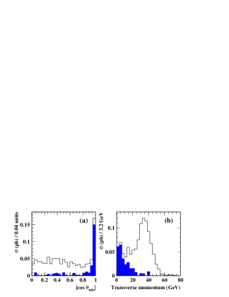
Figure 9: Examples of the momentum imbalance in candidate events for the $\mathrm{W^{+}W^{-}}$$\rightarrow$$\mathrm{q\overline{q}}$$l\nu$ channel: (a) direction of the missing momentum, (b) total momentum transverse to the beam direction. The open histogram indicates events which contain an isolated, identified lepton and pass all other selection cuts; the background from the $\mathrm{Z}/\gamma$, $\mathrm{ZZ}$, $\mathrm{Zee}$ and $\mathrm{We}\nu$ channels is shaded. All samples include detector simulation.

Additional improvements to the selection may be obtained by applying a kinematic fit, in which energy-momentum constraints are applied in conjunction with assumptions about the W masses. The background events tend to give poor probabilities in the fit.

Selection cuts based on these quantities give efficiencies of 70–75% for the $\mathrm{q\overline{q}}$$\mathrm{e}\nu$ and $\mathrm{q\overline{q}}$$\mu\nu$ channels, but only about 5% for the $\mathrm{q\overline{q}}$$\tau\nu$ decays. The purity of the selected sample is 90–95%, with typical accepted cross-sections as listed in Table 7. The corresponding statistical uncertainty on $M_{\mathrm{W}}$ is approximately 200 MeV for 100 pb^-1. More work will be needed to improve the efficiency for selecting $\tau$ decays, and hence to enhance the statistical precision of the cross-section measurement. Hadronic $\tau$ decays can be identified as a third jet with low multiplicity and a small opening angle.

2.2.3 Fully leptonic channel, $\mathrm{W^{+}W^{-}}$$\rightarrow$$l\nu$$l\nu$.

The fully leptonic channel is not used by the direct reconstruction method due to the lack of sufficient constraints on the kinematics of the event, but it can be used for event-counting in the threshold measurement of $M_{\mathrm{W}}$. It has, however, a branching ratio of only 11% ($l=\mathrm{e},\mu,\tau$), a factor 4 lower than the other two channels. This is reflected in the relative weight of this channel to the overall precision on $M_{\mathrm{W}}$ using the threshold method.

The $\mathrm{W^{+}W^{-}}$$\rightarrow$$l\nu$$l\nu$  channel is characterised by two acoplanar, energetic leptons and large missing momentum. In 4/9 (1/9) of the cases, however, one (both) of these leptons is a $\tau$, which typically decays to a narrow hadronic jet. Typical experimental selections for all $\mathrm{W^{+}W^{-}}$$\rightarrow$$l\nu$$l\nu$ channels require:

• Low charged multiplicity (typically not greater than 6), which allows the rejection of most of the hadronic backgrounds. The most important background to this channel is then given by dilepton ($\mathrm{Z}/\gamma$, two-photon or Bhabha) events. At least two good charged tracks (with a typical minimum energy of 1 GeV) are required in any case.

• One identified electron or muon (requiring two would lose most of the events with one $\mathrm{W}\rightarrow\tau\nu_{\tau}$ decay); this lepton is required to have an angle of typically at least $25^{\circ}$ to the beam axis, as both Bhabhas and two-photon events are concentrated at low angles. Since the leptons from $\mathrm{W^{+}W^{-}}$ decays at threshold have approximately half the beam energy, an energy window may be imposed on the lepton, centered around this value (such as [28–55] GeV); this is effective both against low-energy two-photon events (which can be further reduced by requiring a large total visible mass), and against di-muons and Bhabhas, where the energy of each lepton is typically equal to the beam energy.

• Explicit tagging of events with isolated, energetic photons or luminosity clusters allows one to reject radiative Z events with hard, detected ISR.

• Cuts on the missing momentum and its direction can also be used: large transverse missing momentum (typically more than 4 GeV) is required to discriminate against two-photon events, while combined cuts on the angle between the jets and on the missing momentum out of the beam-thrust plane are very effective against di-tau $\mathrm{Z}/\gamma$ events.

• To reconstruct the two original lepton directions, the event is forced into two jets, which must be of low invariant mass and well contained in the detector. A cut on the acoplanarity $\Delta\phi$ between these two jets (such as $\Delta\phi<174^{\circ}$) is effective against all residual backgrounds. The distribution of this variable for signal and background events is shown in Fig. 10.

Selection cuts of this kind give overall efficiencies of approximately 60% (60% to 70% in all individual channels except the $\tau\nu_{\tau}\tau\nu_{\tau}$ channel, where it is only of the order of 30%), with a purity close to 95%. Typical accepted cross-sections are listed in Table 7. The corresponding statistical error on $M_{\mathrm{W}}$ is approximately 360 MeV (354 MeV from signal statistics plus 74 MeV from background statistics) for a total integrated luminosity of 100 $\mathrm{pb}^{-1}$.

Figure 10: Distribution of the jet acoplanarity $\Delta\phi$, in the selection of $\mathrm{W^{+}W^{-}}$$\rightarrow$$l\nu$$l\nu$ events at threshold. The solid histogram includes the events selected by all cuts (except that on $\Delta\phi$). The shaded area corresponds to the background from the $\mathrm{Z}/\gamma$ and $\gamma\gamma$ dilepton events.

2.3 Systematic errors

Uncertainties in the $\mathrm{W^{+}W^{-}}$ production cross-section translate directly into systematic errors on the W mass. The uncertainties fall into three categories: multiplicative uncertainties in the cross-section; an additive uncertainty due to background subtraction; other sources, for example beam energy and W width.

2.3.1 Luminosity, higher-order corrections and selection efficiency

Quantities which enter multiplicatively in the calculation or measurement of the cross-section contribute an error to the W mass which can be expressed as

$$\Delta M_{\mathrm{W}}=\left|\frac{d\sigma}{dM_{\mathrm{W}}}\right|^{-1}\sigma\mbox{\hskip 5.69046pt}\frac{\Delta\mathrm{C}}{\mathrm{C}},$$ (32)

where $\Delta$C is the uncertainty on the multiplicative quantity C, and the cross-section $\sigma$ includes contributions from signal and background weighted by their relative efficiencies. The quantity $\sigma|d\sigma/dM_{\mathrm{W}}|^{-1}$ is shown in Fig. 7 as a function of $\sqrt{s}$. Like the statistical sensitivity factor, it also has a minimum near the nominal threshold and has the value of approximately 1.7 GeV at $(\sqrt{s})^{\,\mathrm{opt}}\simeq 161$ GeV.

The three most important uncertainties of this type are:

• The luminosity, which is expected to be known to about $0.5\%$, including both the known theoretical error on the Bhabha cross-section and the expected experimental error, thus contributing about 8 MeV to $\Delta M_{\mathrm{W}}$.

• Unknown higher-order corrections to the theoretical cross-section (see Section 1.1.6 and Ref. [18]), which if we conservatively assume a value of $\pm 2\%$, contribute about 34 MeV to $\Delta M_{\mathrm{W}}$.

• Uncertainties in the signal efficiency, described in Section 2.3.4 below, which depend on the particular decay channel under consideration.

2.3.2 Background subtraction

An uncertainty $\Delta\sigma_{\mathrm{bkgd}}$ on the residual background cross-section predicted by Monte Carlo propagates as an additive uncertainty to the measured $\mathrm{W^{+}W^{-}}$ cross-section, from which the background has to be subtracted. It contributes an error

$$\Delta M_{\mathrm{W}}=\left|\frac{d\sigma}{dM_{\mathrm{W}}}\right|^{-1}\frac{\Delta\sigma_{\mathrm{bkgd}}}{\epsilon_{WW}}$$ (33)

where $\epsilon_{WW}$ is the signal efficiency, which is found by multiplying the selection efficiency for a given channel by the appropriate branching ratio. The quantity $|d\sigma/dM_{\mathrm{W}}|^{-1}$ is shown in Fig. 7 as a function of $\sqrt{s}$, and is approximately 470 MeV pb^-1 at $(\sqrt{s})^{\,\mathrm{opt}}\simeq 161$ GeV. Experimental methods for determining the uncertainty in the background are described in Section 2.3.4 below. A systematic contribution to $\Delta M_{\mathrm{W}}$ of about 59 MeV (32 MeV) in the $\mathrm{W^{+}W^{-}}$$\rightarrow$$\mathrm{q\overline{q}}$$\mathrm{q\overline{q}}$ ($\mathrm{W^{+}W^{-}}$$\rightarrow$$\mathrm{q\overline{q}}$$l\nu$, $\mathrm{W^{+}W^{-}}$$\rightarrow$$l\nu$$l\nu$) channels is expected.

2.3.3 Beam energy and W width

The error introduced by an uncertainty in the beam energy $E_{\mathrm{beam}}$ to $M_{\mathrm{W}}$ is

$$\Delta M_{\mathrm{W}}=\left|\frac{d\sigma}{dM_{\mathrm{W}}}\right|^{-1}\left|\frac{d\sigma}{d\mbox{$E_{\mathrm{beam}}$}}\right|\Delta\mbox{$E_{\mathrm{beam}}$}.$$ (34)

In the threshold region the cross-section $\sigma_{WW}$ is essentially a function of the single variable $\sqrt{s}-2M_{\mathrm{W}}$ only (see Fig. 6), and hence the ratio of derivatives in (34) is approximately unity, i.e. $\Delta M_{\mathrm{W}}\simeq 1.0\;\Delta\mbox{$E_{\mathrm{beam}}$}$. It is estimated that the beam energy will be known to an accuracy of 12 MeV.

The error on $M_{\mathrm{W}}$ introduced by an uncertainty in the W width $\Gamma_{\mathrm{W}}$ is

$$\Delta M_{\mathrm{W}}=\left|\frac{d\sigma}{dM_{\mathrm{W}}}\right|^{-1}\left|\frac{d\sigma}{d\Gamma_{\mathrm{W}}}\right|\Delta\Gamma_{\mathrm{W}}\simeq 0.16\;\Delta\Gamma_{\mathrm{W}},$$ (35)

where the value of the ratio of the derivatives corresponds to $\sqrt{s}=161~{}$GeV. In the Standard Model, $\Gamma_{\mathrm{W}}$ is proportional to the third power of $M_{\mathrm{W}}$,

$$\Gamma_{\mathrm{W}}=2.080\;\left({M_{\mathrm{W}}\over 80.26\;\mathrm{GeV}}\right)^{3}.$$ (36)

If the current world average value of $M_{\mathrm{W}}=80.26\pm 0.16$ GeV is used then $\Delta\Gamma_{\mathrm{W}}=12$ MeV. In contrast, a (combined) measurement of $\Gamma_{\mathrm{W}}$ by the CDF and D0 collaborations at the Tevatron $\mathrm{p}\bar{\mathrm{p}}$ collider [42] gives $\Gamma_{\mathrm{W}}=2.051\pm 0.061\mbox{(expt.)}\pm 0.013\mbox{(input)}$ GeV, consistent with the Standard Model calculation, but with a much larger error. If we use the Standard Model width, then the contribution (2 MeV) to $\Delta M_{\mathrm{W}}$ is negligible. See Ref. [17] for a further discussion.

2.3.4 Experimental determination of systematic uncertainties

Two methods have been proposed to determine the uncertainty in the signal efficiency and background cross-section. The first method examines the sensitivity of the signal efficiencies and background cross-section to uncertainties in fragmentation. Some preliminary studies have been performed in the $\mathrm{W^{+}W^{-}}$$\rightarrow$$\mathrm{q\overline{q}}$$\mathrm{q\overline{q}}$ channel by varying the fragmentation parameters Q₀, $\sigma_{q}$, $b$ and $\Lambda_{\mathrm{QCD}}$ [43] within one standard error bounds, and noting the effect on the signal efficiency and background cross-section in PYTHIA [43] generated events.

The second method uses data and Monte Carlo event samples from LEP1 to determine the uncertainty in the background cross-section. The selections described in Section 2.2 have been scaled to the LEP1 centre-of-mass energy and applied to both real and simulated data. The difference between data and Monte Carlo gives the error on the background cross-section at $\sqrt{s}\simeq M_{\mathrm{Z}}$. The results are then rescaled to $\sqrt{s}=161$ GeV. It is assumed that the fractional uncertainty on the selection efficiencies for the background is the same at the two energies.

The uncertainty on the signal efficiency appears small from the results of the fragmentation test, within the low statistics of the event samples tested. Further studies are needed to quantify any effects. Therefore a conservative estimate of the signal efficiency error of 2% is used at present, contributing an error of 34 MeV to $M_{\mathrm{W}}$. The uncertainty on the background cross-section in the $\mathrm{W^{+}W^{-}}$$\rightarrow$$\mathrm{q\overline{q}}$$\mathrm{q\overline{q}}$ channel (8%) is estimated to contribute about 59 MeV to the error on $M_{\mathrm{W}}$. The uncertainty in the $\mathrm{W^{+}W^{-}}$$\rightarrow$$\mathrm{q\overline{q}}$$l\nu$ and $\mathrm{W^{+}W^{-}}$$\rightarrow$$l\nu$$l\nu$ channels, estimated to be 50% and 100% respectively, both give an error of about 32 MeV. These errors are expected to decrease with further study.

2.3.5 Conclusions

Table 8 summarizes the estimated systematic errors for the $\mathrm{W^{+}W^{-}}$$\rightarrow$$\mathrm{q\overline{q}}$$\mathrm{q\overline{q}}$, $\mathrm{W^{+}W^{-}}$$\rightarrow$$\mathrm{q\overline{q}}$$l\nu$ and $\mathrm{W^{+}W^{-}}$$\rightarrow$$l\nu$$l\nu$ channels.

Source	$\mathrm{W^{+}W^{-}}$$\rightarrow$$\mathrm{q\overline{q}}$$\mathrm{q\overline{q}}$	$\mathrm{W^{+}W^{-}}$$\rightarrow$$\mathrm{q\overline{q}}$$l\nu$	$\mathrm{W^{+}W^{-}}$$\rightarrow$$l\nu$$l\nu$
Luminosity (*)	8	8	8
HO corrections (*)	34	34	34
Beam energy (*)	12	12	12
W width (*)	2	2	2
Signal efficiency	34	34	34
Background cross-section	59	32	32
Total (MeV)	77	60	60

Table 8: Summary of systematic error contributions, in MeV, to the threshold measurement in the $\mathrm{W^{+}W^{-}}$$\rightarrow$$\mathrm{q\overline{q}}$$\mathrm{q\overline{q}}$, $\mathrm{W^{+}W^{-}}$$\rightarrow$$\mathrm{q\overline{q}}$$l\nu$ and $\mathrm{W^{+}W^{-}}$$\rightarrow$$l\nu$$l\nu$ channels. The quantities denoted (*) are common to all channels. The total for each channel is found by combining the sources in quadrature.

2.4 Summary

Table 9 summarizes the results presented above for the estimated statistical, systematic and total errors on $M_{\mathrm{W}}$ (for all decay channels combined) using the threshold method, i.e. by measuring the $\mathrm{W^{+}W^{-}}$ cross-section at the optimal collider energy of 161 GeV. Our estimates for some of the systematic errors, for example the unknown higher-order theoretical corrections, are probably too conservative, and others, for example the uncertainty in the estimates of the various background cross-sections, will almost certainly decrease with more study. Nevertheless, for the amount of luminosity likely to be available for the threshold measurement the overall error is dominated by statistics.

Total luminosity	$\Delta M_{\mathrm{W}}$ (stat)	$\Delta M_{\mathrm{W}}$ (stat$+$sys1)	$\Delta M_{\mathrm{W}}$ (total)
$4\times 25\;{\rm pb}^{-1}=100\;{\rm pb}^{-1}$	134	139	144
$4\times 50\;{\rm pb}^{-1}=200\;{\rm pb}^{-1}$	95	101	108
$4\times 100\;{\rm pb}^{-1}=400\;{\rm pb}^{-1}$	67	76	84

Table 9: Summary of statistical and systematic errors (in MeV) on $M_{\mathrm{W}}$ from a cross-section measurement (all channels) at $\sqrt{s}=161$ GeV. The total luminosity refers to four experiments combined. The third column includes the channel-dependent systematic errors only (see Table 8), and the fourth column includes the overall common systematic error.

3 Direct Reconstruction of $M_{\mathrm{W}}$

In this section, we discuss the measurement of the W mass by kinematic reconstruction of the invariant mass of the W decay products. The statistical precision of this method which could be obtained by combining four experiments each with 500 pb^-1 at $\sqrt{s}=175\;{\rm GeV}$, assuming 100% efficiency and perfect detector resolution, is about $10\;{\rm MeV}$, limited by the finite width of the W. In practice, this ideal precision will be degraded, partly through loss of statistics, but mainly because detector effects limit the resolution on the reconstructed mass. This has been studied in detail by the four experiments, using Monte Carlo events with full detector simulation. We discuss methods of improving the mass resolution over that obtained by simple calculation of invariant masses. In particular, a kinematic fit using the constraints of energy and momentum conservation, together with the equality of the two W masses in an event, proves to be a very powerful technique for improving the mass resolution, and also turns out to be a useful background rejection criterion. For this reason, we concentrate on the channels $\mathrm{W^{+}W^{-}}$$\rightarrow$$\mathrm{q\overline{q}}$$\mathrm{q\overline{q}}$ and $\mathrm{W^{+}W^{-}}$$\rightarrow$$\mathrm{q\overline{q}}$$l\nu$ where the lepton is an electron or muon, for which constrained fits are most useful.

We start by discussing the basic selection of W-pair events in these two channels, and the reconstruction of jets. We discuss the techniques of the constrained fit in some detail, followed by the determination of $M_{\mathrm{W}}$ from the distribution of reconstructed masses, indicating the statistical error which may be expected. Finally we describe the main sources of systematic error pertaining to this measurement.

3.1 Event selection and jet reconstruction

The criteria used to select W-pair events are essentially the same as those described in Section 2, but at the higher energies used for direct reconstruction the background from Z/$\gamma\rightarrow$$\mathrm{q\overline{q}}$ is lower, so looser cuts can be used.

3.1.1 $\mathrm{W^{+}W^{-}}$$\rightarrow$$\mathrm{q\overline{q}}$$\mathrm{q\overline{q}}$

$\mathrm{W^{+}W^{-}}$$\rightarrow$$\mathrm{q\overline{q}}$$\mathrm{q\overline{q}}$ events are characterised by high multiplicity (about twice that of a Z/$\gamma\rightarrow$$\mathrm{q\overline{q}}$ event at LEP1), high visible energy, and exhibit a four-jet structure. The main background comes from (${\mathrm{Z}^{0}}$/$\gamma)^{*}\rightarrow$$\mathrm{q\overline{q}}$ events, for which the cross-section is much higher, as shown in Table 6. Typical selection cuts for $\mathrm{W^{+}W^{-}}$$\rightarrow$$\mathrm{q\overline{q}}$$\mathrm{q\overline{q}}$ events include:

• high multiplicity of tracks and calorimeter clusters to remove purely leptonic events; a significant fraction of $\mathrm{W^{+}W^{-}}$$\rightarrow$$\mathrm{q\overline{q}}$$l\nu$ and (${\mathrm{Z}^{0}}$/$\gamma)^{*}\rightarrow$$\mathrm{q\overline{q}}$ events can also be removed.

• high visible energy and low missing momentum, to remove $\mathrm{W^{+}W^{-}}$$\rightarrow$$\mathrm{q\overline{q}}$$l\nu$ and radiative Z/$\gamma\rightarrow$$\mathrm{q\overline{q}}$ events.

• explicit removal of events with an isolated electromagnetic cluster consistent with being an initial state photon to remove radiative Z/$\gamma\rightarrow$$\mathrm{q\overline{q}}$ events.

• event shape variables to separate the four-jet $\mathrm{W^{+}W^{-}}$$\rightarrow$$\mathrm{q\overline{q}}$$\mathrm{q\overline{q}}$ events from the remaining background, almost entirely composed of non-radiative Z/$\gamma\rightarrow$$\mathrm{q\overline{q}}$ events. For example, Fig. 11 shows the distribution of $y_{34}^{D}$, the value of $y_{cut}$ in the Durham (k_T) jet-finding scheme at which events change from three jets to four jets, after cuts on the above quantities have been applied. The $\mathrm{W^{+}W^{-}}$$\rightarrow$$\mathrm{q\overline{q}}$$\mathrm{q\overline{q}}$ events tend to have larger values of this variable than the background. Other event shape variables, such as jet broadening measures can also be used.

Figure 11: Distribution of $y_{34}^{D}$, the value of $y_{cut}$ in the Durham (k_T) jet-finding scheme at which events change from three jets to four jets, after cuts on multiplicity, visible energy and missing momentum have been applied to events at 175 GeV. The solid histogram shows $\mathrm{W^{+}W^{-}}$$\rightarrow$$\mathrm{q\overline{q}}$$\mathrm{q\overline{q}}$ events, the open histogram background, mainly non-radiative (${\mathrm{Z}^{0}}$/$\gamma)^{*}\rightarrow$$\mathrm{q\overline{q}}$ events. The dotted line indicates a typical cut value.

In Table 10 we show values of efficiency, purity, accepted cross-sections and numbers of events produced by typical cuts on these variables. The efficiency of selection cuts tends to fall slightly with energy because as $\sqrt{s}$ is increased the W’s are more boosted and event shape variables have less separating power. The purity can be further enhanced by using kinematic fits, as described below, though at a cost in efficiency.

	$\sqrt{s}$ = 175 GeV		$\sqrt{s}$ = 192 GeV
	Accepted	Events	Accepted	Events
	cross-section (pb)	for 500pb-1	cross-section (pb)	for 500pb-1
After basic selection cuts:
$\mathrm{W^{+}W^{-}}$$\rightarrow$$\mathrm{q\overline{q}}$$\mathrm{q\overline{q}}$	5.3	2650	6.2	3100
(${\mathrm{Z}^{0}}$/$\gamma)^{*}\rightarrow$$\mathrm{q\overline{q}}$	3.1	1550	2.1	1050
(${\mathrm{Z}^{0}}$/$\gamma)^{*}$(${\mathrm{Z}^{0}}$/$\gamma)^{*}$	0.1	50	0.4	200
efficiency	83%		79%
purity	62%		62%
After kinematic fit:
$\mathrm{W^{+}W^{-}}$$\rightarrow$$\mathrm{q\overline{q}}$$\mathrm{q\overline{q}}$	4.5	2250	5.0	2500
(${\mathrm{Z}^{0}}$/$\gamma)^{*}\rightarrow$$\mathrm{q\overline{q}}$	1.8	900	1.2	600
(${\mathrm{Z}^{0}}$/$\gamma)^{*}$(${\mathrm{Z}^{0}}$/$\gamma)^{*}$	0.08	40	0.3	150
efficiency	71%		64%
purity	71%		77%
$\Delta(M_{\mathrm{W}})$ (stat)	73 MeV		74 MeV

Table 10: Typical accepted cross-sections and numbers of events for the signal and main backgrounds for the $\mathrm{W^{+}W^{-}}$$\rightarrow$$\mathrm{q\overline{q}}$$\mathrm{q\overline{q}}$ channel for two values of c.m. energy, determined from Monte Carlo including full detector simulation. Values are given both for basic selection cuts, and after demanding a good kinematic fit. The efficiency, purity and expected statistical error on $M_{\mathrm{W}}$ for an integrated luminosity of 500 pb^-1 are also given.

In order to reconstruct the W mass, a jet-finder is used to force the selected events to contain four jets. Jets are usually reconstructed using both tracks and calorimeter information combined to give the best resolution. The typical jet energy resolution is around 20% for a jet energy of 20 GeV, improving to 15% at an energy of 60 GeV; over this same energy range the angular resolution improves from 4^∘ to 1.3^∘ for jets at 90^∘ to the beam direction. Studies of various jet finders comparing the reconstructed jets with the initial quark directions show no major differences among the commonly used schemes. The W mass may then be reconstructed by forming the invariant mass of pairs of jets. For each event, there are three possible combinations; Monte Carlo studies show that the combination where the two highest energy jets are combined together is rarely the correct one, and combinatorial background can be reduced by discarding this combination. The mass resolution can be improved by using beam energy constraints or kinematic fits, as described in the next section.

3.1.2 $\mathrm{W^{+}W^{-}}$$\rightarrow$$\mathrm{q\overline{q}}$$l\nu$

Figure 12: (a) Momentum spectrum of particles identified as leptons and passing isolation cuts at $161\;{\rm GeV}$. (b) scalar sum of charged particle momentum and electromagnetic calorimeter energy in a 200 mrad cone around high momentum identified electrons and muons at $161\;{\rm GeV}$. (c) and (d) as (a) and (b) for $\sqrt{s}=175\;{\rm GeV}$. In each case the solid histogram shows the contribution from leptons in $\mathrm{W^{+}W^{-}}$$\rightarrow$$\mathrm{q\overline{q}}$$l\nu$ events, the open histogram the background. The dashed lines show possible cuts.

The distinguishing feature of $\mathrm{W^{+}W^{-}}$$\rightarrow$$\mathrm{q\overline{q}}$$\mathrm{e}\nu$ and $\mathrm{W^{+}W^{-}}$$\rightarrow$$\mathrm{q\overline{q}}$$\mu\nu$ events is the presence of a high momentum, isolated lepton. Typical selection cuts for $\mathrm{W^{+}W^{-}}$$\rightarrow$$\mathrm{q\overline{q}}$$\mathrm{e}\nu$ and $\mathrm{W^{+}W^{-}}$$\rightarrow$$\mathrm{q\overline{q}}$$\mu\nu$ events include:

• high multiplicity of tracks and calorimeter clusters to remove purely leptonic events; the multiplicity of $\mathrm{W^{+}W^{-}}$$\rightarrow$$\mathrm{q\overline{q}}$$l\nu$ events is lower than that of $\mathrm{W^{+}W^{-}}$$\rightarrow$$\mathrm{q\overline{q}}$$\mathrm{q\overline{q}}$ events, so suitable cuts do not remove (${\mathrm{Z}^{0}}$/$\gamma)^{*}\rightarrow$$\mathrm{q\overline{q}}$ background in this case.

• the presence of a high momentum, isolated, lepton.

	$\sqrt{s}$ = 175 GeV		$\sqrt{s}$ =192 GeV
	Accepted	Events	Accepted	Events
	cross-section (pb)	for 500pb-1	cross-section (pb)	for 500pb-1
After basic selection cuts:
$\mathrm{W^{+}W^{-}}$$\rightarrow$$\mathrm{q\overline{q}}$$l\nu$ ($l=e$ or $\mu$)	3.1	1550	3.8	1880
$\mathrm{W^{+}W^{-}}$$\rightarrow$$\mathrm{q\overline{q}}$$\tau\nu$	0.2	100	0.4	200
(${\mathrm{Z}^{0}}$/$\gamma)^{*}\rightarrow$$\mathrm{q\overline{q}}$	0.2	100	0.2	100
${\mathrm{Z}^{0}}$ ee	0.2	100	0.3	150
efficiency	77%		74%
purity	83%		80%
After kinematic fit:
$\mathrm{W^{+}W^{-}}$$\rightarrow$$\mathrm{q\overline{q}}$$l\nu$($l=e$ or $\mu$)	3.0	1500	3.4	1700
$\mathrm{W^{+}W^{-}}$$\rightarrow$$\mathrm{q\overline{q}}$$\tau\nu$	0.05	25	0.06	30
(${\mathrm{Z}^{0}}$/$\gamma)^{*}\rightarrow$$\mathrm{q\overline{q}}$	0.04	20	0.05	25
${\mathrm{Z}^{0}}$ ee	0.02	10	0.05	25
efficiency	73%		68%
purity	96%		95%
$\Delta(M_{\mathrm{W}})$ (stat)	72 MeV		93 MeV

Table 11: Typical accepted cross-sections and numbers of events for the signal and main backgrounds for the $\mathrm{W^{+}W^{-}}$$\rightarrow$$\mathrm{q\overline{q}}$$l\nu$ ($l=e$ or $\mu$) channel for two values of c.m. energy, determined from Monte Carlo including full detector simulation. Values are given both for basic selection cuts, and after demanding a good kinematic fit. The efficiency, purity and expected statistical error on $M_{\mathrm{W}}$ for an integrated luminosity of 500 pb^-1 are also given.

An isolated lepton can be identified as an electron or muon with fairly loose, standard experimental cuts with high efficiency ($\sim$95%), though only in a limited acceptance, typically $|\cos(\theta)|<0.93$. For example electrons can be identified using the match between track momentum and energy deposited in the electromagnetic calorimeter, where the pattern of energy deposition is consistent with an electromagnetic shower. Muon identification uses matching between a track in a central tracking chamber and one in outer muon detectors. The lepton momentum spectrum and its degree of isolation, as measured by the total scalar sum of charged particle momentum plus electromagnetic energy in a 200mrad cone around the lepton, are shown in Fig. 12. Typical efficiencies, purities, accepted cross-sections and numbers of events are indicated in Table 11. $\mathrm{W^{+}W^{-}}$$\rightarrow$$\mathrm{q\overline{q}}$$\tau\nu$ events can be selected as above, but instead of requiring an identified electron or muon, searching for a narrow, low multiplicity jet isolated from the other jets.

The W mass can be estimated from these events by simply forming the invariant mass of the hadronic system, scaling to the beam energy, or preferably using the full information in a kinematic fit as described below. In this case, the hadronic system is forced to be two jets, which are reconstructed as in the $\mathrm{W^{+}W^{-}}$$\rightarrow$$\mathrm{q\overline{q}}$$\mathrm{q\overline{q}}$ case. The lepton energy resolution is much better than that for a reconstructed jet, as long as care is taken to include all the electromagnetic energy associated with an electron.

3.2 Constrained fit

After the event has been reconstructed as a number of jets and a number of leptons we next turn to the reconstruction of the W mass from these four fermions, which are treated as individual objects with measurable quantities. We try to reconstruct the best estimator for the W mass on an event by event basis from the measured quantities and the constraints imposed by energy and momentum conservation, and the possible additional constraint that the masses of the two W’s are equal.

Without imposing any constraints the direct reconstruction of the di-jet mass gives:

$$m_{ij}=\sqrt{2E_{i}E_{j}(1-\cos\theta_{ij})},$$ (37)

where $E_{i}$ and $E_{j}$ are the jet energies, $\theta_{ij}$ the jet-jet opening angle and where the jet masses have been neglected. Taking only the errors on the jet energies into account, as these are much larger than the errors on the angle measurements, this then gives:

$$\frac{\sigma(m_{ij})}{m_{ij}}=\sqrt{\left(\frac{\sigma(E_{i})}{2E_{i}}\right)^{2}+\left(\frac{\sigma(E_{j})}{2E_{j}}\right)^{2}}$$ (38)

Typical jet energy measurement errors of 15% at $45\;{\rm GeV}$ lead to a relative uncertainty of 10% on $M_{\mathrm{W}}$, and give distributions of reconstructed mass as shown in the top half of Fig. 13. To make a precision measurement of $M_{\mathrm{W}}$ it is necessary to improve this resolution by making use of the knowledge of the total energy and momentum which is given in an $\mathrm{e^{+}e^{-}}$ collider.

3.2.1 Rescaling methods

These methods are especially useful for the analysis of the semi-leptonic channels and most have been described previously [1]. The basic principle is to write the momentum, energy, and equal mass constraints as functions of the measured fermion momenta and solve for those variables which have the largest measurement uncertainties, generally jet energies.

The first step is to include the beam energy constraint, which is equivalent to the constraint that the two masses are equal:

$$E_{i}+E_{j}=E_{\rm b}.$$ (39)

This leads to a determination of the reconstructed $M_{\mathrm{W}}$:

$$m_{ij}=\frac{E_{\rm b}}{E_{i}+E_{j}}\sqrt{2E_{i}E_{j}(1-\cos\theta_{ij})}.$$ (40)

Assuming that only the errors on the jet energies are important the error on the mass becomes:

$$\frac{\sigma(m_{ij})}{m_{ij}}\simeq\frac{|E_{i}-E_{j}|}{E_{i}+E_{j}}\sqrt{\left(\frac{\sigma(E_{i})}{E_{i}}\right)^{2}+\left(\frac{\sigma(E_{j})}{E_{j}}\right)^{2}}.$$ (41)

Together with the other errors which were neglected, this leads to a relative uncertainty on the reconstructed mass of typically 5%. This method is especially suited to the semi-leptonic channel in which the leptonic W decay into $\tau\nu_{\tau}$ does not allow advantage to be taken of the measured lepton energy.

In the case of semi-leptonic decays to an electron or muon, we can include the parameters of the measured lepton by writing:

$$\vec{p}_{\nu} = -E_{\ell}\vec{{\rm e}_{\ell}}-E_{i}\vec{{\rm e}_{i}}-E_{j}\vec{{\rm e}_{j}}$$

$$E_{i}+E_{j} = E_{\rm b}$$

$$E_{\ell}+E_{\nu} = E_{\rm b},$$ (42)

where $\vec{\rm e}$ are unit vectors in the direction of the particles. These five equations with five unknowns, $\vec{p}_{\nu}$, $E_{i}$, and $E_{j}$, can be solved, and yield two distinct solutions. This ambiguity leads to a problem if the two solutions are close to each other. Taking the solution which is closest to the measured jet energies leads to a relative error on $M_{\mathrm{W}}$ of about 4%.

The two exact solutions of Eq. (42) will give two minima also for the constrained fit in the $\chi^{2}(M_{\mathrm{W}})$ distribution when the two solutions are close. Monte Carlo studies suggest that about 40% of the events are afflicted by this problem. Current analyses have not yet included this effect in the determination of $M_{\mathrm{W}}$ and one might therefore expect an improvement in resolution if this effect is taken correctly into account.

3.2.2 The constrained fit

The most effective way to use all the information available in an event is to perform a constrained kinematic fit. In such a fit, the measured parameters are varied until a solution is found which satisfies the constraints imposed and also minimises the $\chi^{2}$ difference between the measured and fitted values. Several methods exist to perform this minimization. A traditional one solves the problem using Lagrange multipliers, minimising

$${\cal S}(\vec{y},\vec{\lambda})=(\vec{y}-\vec{y_{0}})^{\top}{\bf V}^{-1}(\vec{y}-\vec{y_{0}})+2\vec{\lambda}\cdot\vec{f}(\vec{y}),$$ (43)

where ${\bf V}$ is the error matrix, $\vec{y}$ the fitted variables, $\vec{y_{0}}$ the measured values, $\vec{\lambda}$ Lagrange multipliers, and $\vec{f}(\vec{y})$ the constraints written as functions which must vanish. An equivalent method is to use penalty functions where terms of the type $\vec{f}^{2}/\sigma^{2}$ are added to the $\chi^{2}$. The procedure then minimizes the total $\chi^{2}$ in an iterative way, for each step decreasing the $\sigma$ of the penalties. Results are in general the same but the convergence is slightly slower.

The inputs to the fit are measurements of the energy and angles, of the four jets in the hadronic final state or of the two jets and lepton in the semi-leptonic final state, together with their error matrix. Errors on jet parameters can be extracted from data or Monte Carlo, and may be functions of both energy and position measured in the detector. In practice most of the jet measurement errors are nearly uncorrelated, making the error matrix diagonal. For the jet masses two different strategies are used. Either the jets are assumed to be massless and the measured jet energy is used as the measured jet momentum, or one includes the reconstructed jet masses in the fit. (Note that the $\tau$ lepton can be treated in nearly the same way as jets, except that the errors on the transverse momenta are given by the missing mass and that the $\tau$ mass is used explicitly in the fit. This has not yet been studied in detail.)

The fit can be performed using only the constraints of energy and momentum conservation, or also including the constraint that the masses of the two reconstructed W’s be equal. In the hadronic channel, this gives a 4C or 5C fit respectively. In the semi-leptonic channel, the number of constraints is reduced by three because the parameters of the neutrino are unmeasured, resulting in a 1C or 2C fit. The equal mass constraint can be included exactly, or the width of the W can be taken into account by adding a term to the $\chi^{2}$ proportional to the difference in mass of the two W’s. In practice, because the mass resolution is larger than the W width, both methods give almost the same results. If an equal mass constraint is not applied, the reconstructed masses of the two di-fermion systems are strongly anticorrelated. Thus only the average invariant mass can usefully be extracted per event. The inclusion of an equal mass constraint is preferred over a fit using only energy and momentum conservation because it gives improved mass resolution and superior background rejection.

In the 4-jet channel we do not know which jets are to be combined to produce the heavy particles we are interested in reconstructing. Therefore the constrained fit is performed for all three possible combinations. In the case with no equal mass constraint there are three different mass solutions with the same $\chi^{2}$. When an equal mass constraint is imposed the three different solutions will in general have different $\chi^{2}$ and one can therefore use this information to distinguish between the solutions. The procedure employed by most analyses is to first define a mass window, wide enough not to bias the mass measurement, and if more than one solution exists inside this window choose the solution with the lowest $\chi^{2}$. This procedure is however not perfect and one is left with a fraction of wrong combinations as shown in Fig. 13.

3.2.3 Results of the fit

In Fig. 13 we show invariant mass distributions before and after the fit, in the latter case taking only those events which give a good fit. Before the fit, the mass distributions are very broad. After the fit the mass resolutions obtained are typically 3.5% for the $\mathrm{W^{+}W^{-}}$$\rightarrow$$\mathrm{q\overline{q}}$$l\nu$ channel and around 2.5% for the 4-jet channel. It is also clear from this figure that the $\chi^{2}$ of the constrained fit can be used to eliminate possible background which does not comply with the $\mathrm{W^{+}W^{-}}$ hypothesis: the level of background is much lower in both channels after demanding a good fit. However, a fraction of $\mathrm{W^{+}W^{-}}$ events, varying from about 10% to 30% depending on the channel, also fails to give a good fit. These events are discussed below. Typical values of efficiency and purity after the fit are given in Tables 10 and 11.

Figure 13: Distributions of the invariant mass for selected events for the $\mathrm{W^{+}W^{-}}$$\rightarrow$$\mathrm{q\overline{q}}$$\mathrm{q\overline{q}}$ channel at $\sqrt{s}=192\;{\rm GeV}$ (left) and the $\mathrm{W^{+}W^{-}}$$\rightarrow$$\mathrm{q\overline{q}}$$l\nu$ channel at $\sqrt{s}=175\;{\rm GeV}$ (right). The top plots are before the kinematic fit, the bottom ones after a five-constraint ($\mathrm{W^{+}W^{-}}$$\rightarrow$$\mathrm{q\overline{q}}$$\mathrm{q\overline{q}}$) or two-constraint ($\mathrm{W^{+}W^{-}}$$\rightarrow$$\mathrm{q\overline{q}}$$l\nu$) kinematic fit. For the $\mathrm{W^{+}W^{-}}$$\rightarrow$$\mathrm{q\overline{q}}$$\mathrm{q\overline{q}}$ channel, the open histograms show the correctly found jet-jet combinations, the singly hatched areas correspond to the incorrectly found jet-jet combinations and the cross-hatched parts indicate the background from other sources (mainly $q\bar{q}(\gamma)$). For the $\mathrm{W^{+}W^{-}}$$\rightarrow$$\mathrm{q\overline{q}}$$l\nu$ channel the open histograms show signal events, the cross-hatched areas background including the $\mathrm{W^{+}W^{-}}$$\rightarrow$$\mathrm{q\overline{q}}$$\tau\nu$ contribution. The statistics correspond to an integrated luminosity of 500 pb^-1.

From the constrained fit we can calculate the error on the fitted mass. This error is highly correlated to the actual value of the fitted mass, so selecting events with a simple cut on this quantity would seriously bias the measurement. The reason for this effect is related to the kinematics of the events. When the mass approaches the kinematic limit the precision on the sum of the unknown masses will be better and better while the precision on the difference between the masses will deteriorate. This leads to a mass resolution that broadens with increasing energy. Going from $175\;{\rm GeV}$ to $192\;{\rm GeV}$ typically increases the measurement errors by 25% on an event by event basis. The effect of this on the final statistical error on $M_{\mathrm{W}}$ is diluted by the fixed $\Gamma_{\rm W}$ and compensated by an increase of the $\mathrm{W^{+}W^{-}}$ cross-section.

The constrained fit assumes that the errors on the measured quantities are Gaussian and uncorrelated between jets. Several effects lead to non-Gaussian errors and correlations. Each of these will lead to tails in the distributions and hence to a peak at low probability for the fitted $\chi^{2}$. The most important is gluon radiation, but also overlapping jets, initial state radiation, $\Gamma_{\rm W}$, and acceptance effects play a rôle. The hard gluon radiation is of course in direct disagreement with the treatment of jets as independent objects. Even rather soft gluon radiation lead to jets being broadened in a specific direction, giving correlations that are not included in the current implementations of the constrained fit. Studies have been performed to try to recover some of the 4-jet events which fail to give a good fit by treating them as 5-jet events. However, although some fraction of these events then give a good fit, the combinatorial problem is severe, and it appears that their inclusion has little effect on the ultimate mass resolution.

3.2.4 Inclusion of initial state radiation

As will be seen below, energy lost in initial state radiation biases the fitted mass if it is not included in the fit. Initial state radiation can be included in the constrained fit using the following procedure. We know that there is a large probability that the photon is produced close to the collision axis and hence not detected. We can therefore as a good assumption take the momentum to be collinear with the $z$-axis. We also know to a high precision the expected distribution of the photon energy. In a simple approximation this reads:

$$p(x)dx=\beta x^{\beta-1}dx,$$ (44)

where $x=E_{\gamma}/\sqrt{s}$ and $\beta$ is a parameter which is smaller than unity and depends on $\sqrt{s}$. Since this is non-Gaussian we cannot take this term directly into the $\chi^{2}$ expression. Instead we introduce the likelihood concept and use the standard -2 ln(likelihood) as the term to add to the $\chi^{2}$. If we just use the probability as the likelihood this approach will not work since the distribution has a pole for $x\rightarrow 0$. Instead one can choose to use the confidence limit as an estimator for the likelihood:

$$C(x)=\int_{x}^{\infty}p(y)dy$$ (45)

With this formulation the constrained fit works but its implementation is rather difficult since one has to divide the fit into two parts: one where one assumes the photon goes in the forward direction and one where one assumes the opposite. When the fitted $E_{\gamma}$ approaches zero the first order derivative of $\chi^{2}$ will still diverge, but this only means that the fit prefers the zero solution, since the measurement does not have sufficient resolution to distinguish between no $\gamma_{\rm ISR}$ and a $\gamma_{\rm ISR}$ with a small energy. Monte Carlo studies show that photons below about $3\;{\rm GeV}$ cannot be resolved and when photons are above typically $8\;{\rm GeV}$ the W bosons can not be on mass-shell. The final improvement in the $M_{\mathrm{W}}$ measurement is therefore limited.

3.3 Determination of the mass and width of the W

In this section we describe several strategies for extracting $M_{\mathrm{W}}$ from distributions of reconstructed invariant masses such as those show in Fig. 13. As we aim for a precision measurement of $M_{\mathrm{W}}$ with sub-permille accuracy, this is a non-trivial task, because we have to control any systematic effect to an accuracy of a few MeV. The total width of the W boson, $\Gamma_{\mathrm{W}}$, may either be extracted simultaneously with the mass, or the functional dependence $\Gamma_{\mathrm{W}}=\Gamma_{\mathrm{W}}(M_{\mathrm{W}})$ of the Standard Model may be imposed as a constraint for increased accuracy on $M_{\mathrm{W}}$. The methods to analyse the data in terms of $M_{\mathrm{W}}$ and $\Gamma_{\mathrm{W}}$ fall into four groups: (1) Monte Carlo calibration of simple function; (2) (De-) Convolution of underlying physics function; (3) Monte Carlo interpolation; (4) Reweighting of Monte Carlo events.

In general, all methods make use of Monte Carlo event generators [18] and detector simulation to determine the effects of the detector such as resolution. Thus any method has to be checked for possible systematic biases introduced by using Monte Carlo event samples generated with certain input values for $M_{\mathrm{W}}$ and $\Gamma_{\mathrm{W}}$. In addition, systematic errors may arise due to deficiencies in the Monte Carlo simulation describing the detector and/or the data. Other systematic errors arise from the technical implementation of the fitting methods, such as fit range, bin width in case of binned data, choice of functions to describe signal and background etc.

3.3.1 Monte Carlo calibration

To fit the invariant mass distribution, this method uses a simple, ad-hoc function, e.g., a double Gaussian or a Breit-Wigner convoluted with a Gaussian, to describe the signal peak and another simple function to describe the background. One of the fit parameters is used as an estimator, $M$, for the W mass, e.g., the mean of the Gaussian or the Breit-Wigner. The same fitting procedure is applied to both data and Monte Carlo events. Since for the latter the input W mass, $M_{\mathrm{W}}^{\mathrm{MC}}$, is known, the Monte Carlo result is used to evaluate the bias $\Delta$ of this method, $\Delta\equiv M^{\mathrm{MC}}-M_{\mathrm{W}}^{\mathrm{MC}}$, where this bias may depend on the final state analysed. The mass of the W measured in the data is now simply given by the estimator $M^{\mathrm{data}}$ derived from fitting the data distribution, corrected for the bias $\Delta$ evaluated from Monte Carlo events: $M_{\mathrm{W}}=M^{\mathrm{data}}-\Delta$.

This procedure automatically takes into account all corrections for all biases as long as they are implemented in the Monte Carlo simulation, such as initial-state radiation, background contributions, detector resolutions and efficiencies, selection cuts etc. The knowledge of how well the Monte Carlo describes the underlying physics and the detector response enters in the systematic error on the bias $\Delta$.

The fundamental drawback of this method is that the simple function used in the fit is not unique. Depending on its choice, even different statistical errors on $M_{\mathrm{W}}$ can be obtained. In addition, the estimate of the bias correction $\Delta$ depends itself to some extent on the Monte Carlo parameters $M_{\mathrm{W}}^{\mathrm{MC}}$ and $\Gamma_{\mathrm{W}}^{\mathrm{MC}}$, or on the centre-of-mass energy, $\sqrt{s}$, $\Delta=\Delta(s;M_{\mathrm{W}}^{\mathrm{MC}},\Gamma_{\mathrm{W}}^{\mathrm{MC}})$. Such a dependence, however, can be corrected for by iteration.

3.3.2 Convolution

The drawbacks listed above are alleviated in the convolution method. Here, the correct function, i.e., the underlying physics function, is used as a fitting function. This function is simply the differential cross-section in the two invariant masses (denoted by $m_{1},m_{2}$). Note that this function is not a simple Breit-Wigner distribution in $m_{1}$ and $m_{2}$ due to phase space effects and radiative corrections. Several analytical codes exist (e.g., GENTLE etc. [18]), which calculate the differential cross-section including QED corrections, $\frac{\mathrm{d^{2}\,}\sigma(s;M_{\mathrm{W}},\Gamma_{\mathrm{W}})}{\mathrm{d\,}m_{1}\mathrm{d\,}m_{2}}$, as a function of the centre-of-mass energy, $\sqrt{s}$, and the Breit-Wigner mass and total width of the W boson, $M_{\mathrm{W}}$ and $\Gamma_{\mathrm{W}}$.

The effects of the detector are included by convolution. The prediction for the distribution of the reconstructed invariant masses (denoted by $\overline{m}_{1},\overline{m}_{2}$) is thus given by:

$$\frac{\mathrm{d^{2}\,}\sigma(s;M_{\mathrm{W}},\Gamma_{\mathrm{W}})}{\mathrm{d\,}\overline{m}_{1}~{}\mathrm{d\,}\overline{m}_{2}}~{}=~{}\int\mathrm{d\,}m_{1}\int\mathrm{d\,}m_{2}~{}G(s;\overline{m}_{1},\overline{m}_{2},m_{1},m_{2})\cdot\frac{\mathrm{d^{2}\,}\sigma(s;M_{\mathrm{W}},\Gamma_{\mathrm{W}})}{\mathrm{d\,}m_{1}~{}\mathrm{d\,}m_{2}}\,.$$ (46)

The transfer or Green’s function $G$, which depends on the final state analysed, can be interpreted as the probability of reconstructing the pair of invariant masses $(\overline{m}_{1},\overline{m}_{2})$ given the event contained the pair of true invariant masses $(m_{1},m_{2})$. Several simplifications for $G$ are possible, down to a 1-dimensional resolution function $G=G\left([{\overline{m}_{1}+\overline{m}_{2}}]/{2}-[{m_{1}+m_{2}}]/{2}\right)$.

The actual fitting of invariant mass distributions can be performed either on the measured or on unfolded distributions. In the former case, the underlying physics function, $\frac{\mathrm{d^{2}\,}\sigma(s;M_{\mathrm{W}},\Gamma_{\mathrm{W}})}{\mathrm{d\,}m_{1}\mathrm{d\,}m_{2}}$, is convoluted with $G$, and the result is fitted to the data with $M_{\mathrm{W}}$ and $\Gamma_{\mathrm{W}}$ as fit parameters. In the latter case, the measured distribution, $\frac{\mathrm{d^{2}\,}\sigma(s;M_{\mathrm{W}},\Gamma_{\mathrm{W}})}{\mathrm{d\,}\overline{m}_{1}\mathrm{d\,}\overline{m}_{2}}$, is first unfolded for detector effects, by applying the “inverse” of $G$. The underlying physics function, $\frac{\mathrm{d^{2}\,}\sigma(s;M_{\mathrm{W}},\Gamma_{\mathrm{W}})}{\mathrm{d\,}m_{1}\mathrm{d\,}m_{2}}$, can now be fitted directly to the unfolded distribution. From a purely mathematical point of view, both methods are equivalent. In practice, however, $G$ is determined only up to a certain statistical accuracy. Since folding is an intrinsically stable procedure in contrast to unfolding, which is unstable, the former method is preferred. Reference [49] gives more details on the features of unfolding procedures. Backgrounds are described by simple functions, derived from data and from Monte Carlo simulations, which are added to the signal.

This method allows cuts on generated invariant masses ($m_{1},m_{2}$) and ISR energy loss, since these are the only variables used in most semianalytical codes. In addition, cuts on the reconstructed invariant masses ($\overline{m}_{1},\overline{m}_{2}$) are possible. Since cuts on other variables cannot be applied, it must be checked whether selection cuts bias the invariant mass distribution, for example by testing the method with Monte Carlo events (cf. method (1)).

3.3.3 Other Monte Carlo based methods

The problems of the previous two methods can be solved by a Monte Carlo interpolation technique. Several samples of Monte Carlo events corresponding to different input values of $M_{\mathrm{W}}^{\mathrm{MC}}$ and $\Gamma_{\mathrm{W}}^{\mathrm{MC}}$ are simulated, e.g., in a grid around the current central values for $(M_{\mathrm{W}},\Gamma_{\mathrm{W}})$ extending a few times the total (expected) error in all directions. The Monte Carlo samples of the accepted events are compared to the accepted data events, thereby taking the influence of event selection cuts into account. Backgrounds are included by adding the corresponding Monte Carlo events. The compatibility of the invariant mass distributions is calculated, e.g., in terms of a $\chi^{2}$ quantity. Interpolation of the $\chi^{2}$ within the generated ($M_{\mathrm{W}}^{\mathrm{MC}}$, $\Gamma_{\mathrm{W}}^{\mathrm{MC}}$) grid allows to find the values $M_{\mathrm{W}}$ and $\Gamma_{\mathrm{W}}$ which minimise the $\chi^{2}$. Like method (1), this method corrects automatically all possible biases due to all effects considered in the Monte Carlo simulation. The only drawback is that a rather large amount of Monte Carlo events must be simulated.

This problem, however, can be solved by a reweighting procedure. In that case only one sample of Monte Carlo events is needed, which has been generated with fixed values $M_{\mathrm{W}}^{\mathrm{MC}}$ and $\Gamma_{\mathrm{W}}^{\mathrm{MC}}$. Event-by-event reweighting in the generated invariant masses ($m_{1},m_{2}$) is performed to construct the prediction for the invariant mass distributions corresponding to values $M_{\mathrm{W}}^{\mathrm{fit}}$ and $\Gamma_{\mathrm{W}}^{\mathrm{fit}}$. These distributions are then fitted to the data distributions. Since individual Monte Carlo events are reweighted, it is straight forward to implement the effects of selection cuts. Moreover, using a Monte Carlo generator also in the calculation of the event weights, it is even possible to extend further the set of variables on which the event weights depend to include any kinematic variable describing the four-fermion final state, such as the reconstructed fermion energies and angles.

3.3.4 Expected statistical error on $M_{\mathrm{W}}$

So far the experiments have studied methods (1), (2) and (3) [44, 45, 46, 47]. For the statistical errors on $M_{\mathrm{W}}$ quoted in Tables 10 and 11, the experiments have mainly used method (1), which is adequate for this purpose. It should be noted that the more involved analyses (2), (3) and (4) do not aim for a reduction in the statistical error on $M_{\mathrm{W}}$. This error is fixed by the number of selected events, the natural width of the W boson and the detector resolution in invariant masses. Instead the advantage of these methods lies in the fact that they allow a thorough investigation of the various systematic biases arising in the determination of the W mass. It is possible to disentangle systematic effects due to background diagrams, initial-state radiation, event selection, detector calibration and resolution etc. Thus, in order to have a better control of systematic effects, it is envisaged that the final analyses will use the more involved strategies (2), (3), (4) or a combination thereof.

As shown in Table 10, the statistical error on $M_{\mathrm{W}}$ from the $\mathrm{W^{+}W^{-}}$$\rightarrow$$\mathrm{q\overline{q}}$$\mathrm{q\overline{q}}$ channel is expected to be about $73\;{\rm MeV}$, roughly independent of $\sqrt{s}$, for an integrated luminosity of $500\;{\rm pb}^{-1}$. For the $\mathrm{W^{+}W^{-}}$$\rightarrow$$\mathrm{q\overline{q}}$$l\nu$ channel a similar value is expected at $175\;{\rm GeV}$, but at higher energies the worsening resolution on $M_{\mathrm{W}}$ causes this value to increase somewhat.

3.4 Systematic errors

Three classes of systematic error have been envisaged: errors coming from the accelerator, from the knowledge of the underlying physics phenomena, and from the detector. The last two classes are sometimes related as some physics parameters may affect the detector response. In contrast with the threshold cross-section method, effects which distort the mass distribution must be considered here. Most of the following error estimates have been obtained using simulations. The models used will be checked against LEP2 data when available and represent today’s state of the art.

3.4.1 Error from the LEP beam

The direct mass reconstruction method relies on constraining or rescaling the energies of the reconstructed W’s to the beam energy. The error on the beam energy is foreseen to be less than $12\;{\rm MeV}$ (see Section 1.1), translating to $12\;{\rm MeV}\ \times M_{\mathrm{W}}/E_{beam}$ on the mass. The beam energy spread will be $\approx 40\;{\rm MeV}\times s/(91\;{\rm GeV})^{2}$  [2] with a negligible effect on the statistical error. The operation with bunch trains should not significantly affect the beam energy. Experience gained at LEP1 will guarantee a very good follow up of the behaviour of the beam even at short time scales.

3.4.2 Error from the theoretical description

The most important distortion of the mass distribution comes from initial state radiation (ISR). The average energy carried by radiated ISR photons is $\langle E_{ISR}\rangle=1.2\;{\rm GeV}$ per event at $\sqrt{s}=175\;{\rm GeV}$ and rises linearly up to $2.2\;{\rm GeV}$ at $\sqrt{s}=200\;{\rm GeV}$. From the beam energy constraint, one expects an average mass shift of the order of $\langle E_{ISR}\rangle M_{\mathrm{W}}/\sqrt{s}$, i.e. about $500\;{\rm MeV}$ at $175\;{\rm GeV}$. A fit to the mass distribution gives more weight to the peak yielding a shift of only $200\;{\rm MeV}$ at this energy. As a direct measurement of the ISR spectrum seems impossible to an accuracy relevant for the W mass measurement, we will rely on the theoretical calculations as described in Section 1.6.5 which present an error of $10\;{\rm MeV}$ on $\langle E_{ISR}\rangle$. Together with uncertainties on the shape of the spectrum, this translates into an error smaller than $10\;{\rm MeV}$ on the W mass.

Background events contained in the final sample will also distort the mass distribution (Fig. 13). These backgrounds can be monitored with the data themselves under a dedicated analysis. The most important source of background comes from (${\mathrm{Z}^{0}}$/$\gamma)^{*}\rightarrow$$\mathrm{q\overline{q}}$ events which has a flat mass distribution in the fit area. The effects of an error on the level or in the shape of this background have been estimated by changing its production cross-section by 20% and by shifting the background mass distribution by $0.5\;{\rm GeV}$ resulting in an error of $12\;{\rm MeV}$ for the $\mathrm{W^{+}W^{-}}$$\rightarrow$$\mathrm{q\overline{q}}$$\mathrm{q\overline{q}}$ channel and $6\;{\rm MeV}$ for the $\mathrm{W^{+}W^{-}}$$\rightarrow$$\mathrm{q\overline{q}}$$l\nu$ channel. The background four jet rate as measured at LEP1 is not perfectly reproduced by the simulations [50] and will have to be better determined.

The fragmentation model for W events is the same as was fitted to Z events at LEP1. To estimate errors from this model, each of its parameters has been varied and the error is derived according to a 1 standard deviation from the best fit value. The total error is $16\;{\rm MeV}$, which should be taken as an upper limit as the parameters have been varied separately without taking into account correlations.

Colour reconnection and Bose-Einstein correlations may seriously affect the mass distribution in the $\mathrm{W^{+}W^{-}}$$\rightarrow$$\mathrm{q\overline{q}}$$\mathrm{q\overline{q}}$ channel. These are discussed in detail in Section 4.

3.4.3 Error from the detector

Effects of miscalibration appear to be very small. This is due to the use of the beam energy which gives a precise scale. For instance, a conservative shift of 2% in the momentum of charged tracks, and miscalibration of 5% for electromagnetic and hadronic calorimeters produces a shift of $10\;{\rm MeV}$ on the W mass.

During the LEP2 era, it is foreseen to run for short periods at $\sqrt{s}=\mbox{$M_{\mathrm{Z}}$}$ in order to calibrate and determine the efficiencies of the detectors with high statistics. Genuine LEP2 events like $\mbox{$\mathrm{e^{+}e^{-}}$}\rightarrow\mbox{${\mathrm{Z}^{0}}$}\gamma$ will also be used to monitor the hadronic recoil mass to the photon. Two Z events produced at LEP1 can be mixed and boosted to a LEP2 energy to study the adequacy of the mass reconstruction in comparison with the simulations.

In the $\mathrm{W^{+}W^{-}}$$\rightarrow$$\mathrm{q\overline{q}}$$\mathrm{q\overline{q}}$ channel, the wrong assignment of a jet to a W distorts the mass distribution giving rise to a low mass tail. The amount of such misassignments depends on the algorithms used. By changing parameters in such algorithms we estimate an error of up to $5\;{\rm MeV}$.

Several methods to extract the W mass from the measurements have been studied (see Section 3.3). If a simple function is fitted to the measured mass distribution, errors from the choice of the mass fit range are to be expected, and are typically $10\;{\rm MeV}$. A convolution of the physics function with (or a deconvolution from) detector effects should largely reduce such errors. However this convolution depends on the accuracy of the simulation of the event structure, for instance on the fragmentation model used (see above).

In the present simulation studies, limited statistics have been generated. The statistical error on the mass shift with 500k events simulated is of the order of $10\;{\rm MeV}$.

Source	$\mathrm{W^{+}W^{-}}$$\rightarrow$$\mathrm{q\overline{q}}$$\mathrm{q\overline{q}}$	$\mathrm{W^{+}W^{-}}$$\rightarrow$$\mathrm{q\overline{q}}$$l\nu$
$E_{beam}$	12	12
ISR	10	10
fragmentation	16	16
backgrounds	12	6
calibration	10	10
MC statistics	10	10
mass fit	10	10
jet assignment	5	-
interconnection	?	-
total	31	29

Table 12: Estimated systematic errors on $M_{\mathrm{W}}$ per experiment in$\;{\rm MeV}$. Colour reconnection and Bose-Einstein effects are not included in the total.

3.4.4 Common errors

The effects mentioned above are summarized in Table 12 and total to about $30\;{\rm MeV}$ for each channel at $\sqrt{s}=175\;{\rm GeV}$. Although errors from the beam energy, ISR and background will vary with energy, we do not expect large variations over the 165 to $190\;{\rm GeV}$ range.

Errors on the beam energy and ISR are common to all experiments. Errors from fragmentation and background are partially common as far as the physical parameters are concerned, but a particular analysis will retain a level of background or be sensitive to fragmentation tails in a different way from another analysis, hence with a slightly different error. If these errors were considered common to the four experiments, they would amount to a total of $25\;{\rm MeV}$ ($23\;{\rm MeV}$) in the $\mathrm{W^{+}W^{-}}$$\rightarrow$$\mathrm{q\overline{q}}$$\mathrm{q\overline{q}}$ ($\mathrm{W^{+}W^{-}}$$\rightarrow$$\mathrm{q\overline{q}}$$l\nu$) channel.

3.5 Summary

In Table 13 we show the total error on $M_{\mathrm{W}}$ which might be expected by combining four experiments each with an integrated luminosity of $500\;{\rm pb}^{-1}$ at $\sqrt{s}=175\;{\rm GeV}$. As discussed in the previous section, systematic errors from the beam energy measurement and initial state radiation, fragmentation and backgrounds are considered common to both channels and to all experiments. The total expected error is around $34\;{\rm MeV}$. with roughly equal contributions from statistics and systematics. This value is expected to rise, but only very slowly, with $\sqrt{s}$ because of the worsening mass resolution.

Source	$\mathrm{W^{+}W^{-}}$$\rightarrow$$\mathrm{q\overline{q}}$$\mathrm{q\overline{q}}$	$\mathrm{W^{+}W^{-}}$$\rightarrow$$\mathrm{q\overline{q}}$$l\nu$	Combined
Statistical	36	36	25
Common systematic	25	23	23
Uncorr. systematic	9	9	6
total	45	44	34

Table 13: Estimated total error on $M_{\mathrm{W}}$, in$\;{\rm MeV}$, which could be obtained by combining four experiments each with an integrated luminosity of $500\;{\rm pb}^{-1}$ at $\sqrt{s}=175\;{\rm GeV}$. Colour reconnection and Bose-Einstein effects are not included in the systematic error.

4 Interconnection Effects

4.1 Introduction

The success of the precision measurements of the W boson mass $M_{\mbox{\scriptsize W}}$ strongly relies on accurate theoretical knowledge of the dynamics of the production and decay stages in $\mbox{e}^{+}\mbox{e}^{-}\rightarrow\mbox{W}^{+}\mbox{W}^{-}\rightarrow 4$ fermions. Owing to the large W width, $\Gamma_{\mbox{\scriptsize W}}$, these stages are not independent but may be interconnected by QCD (and electroweak) interference effects, which must be kept under theoretical control. Interconnection phenomena may obscure the separate identities of the two W bosons, so that the final state may no longer be considered as a superposition of two separate W decays [51, 52]. Thus the “direct reconstruction” method of measuring $M_{\mbox{\scriptsize W}}$ at LEP2 using the hadronic $(\mbox{q}_{1}\overline{\mbox{q}}_{2}\,\mbox{q}_{3}\overline{\mbox{q}}_{4})$ channel has an important caveat — the colour reconnection effects [51, 52, 53] — which may distort the mass determination [52]. Another delicate question is whether Bose–Einstein effects could induce a further uncertainty in the mass determination [52, 54].

The hadronic effects mentioned above are all well-known from other processes. Interferences in the production and decay of unstable objects are observed e.g. in multipion final states at low invariant masses [55]. QCD interconnection could be exemplified by J/$\psi$ production in B decay: in the weak decay $\mbox{b}\rightarrow\mbox{c}\mbox{W}^{-}\rightarrow\mbox{c}\,\overline{\mbox{c}}\mbox{s}$ the $\mbox{c}\overline{\mbox{c}}\rightarrow\mbox{J}/\psi$ formation requires a “cross-talk” between the $\overline{\mbox{c}}$$+$s and the c$+$spectator colour singlets. Bose–Einstein effects are readily visible in high-energy multiparticle production, including LEP1. In view of the precedents, the working hypothesis must be that interconnection effects are at play also for W⁺W^- events.

The space–time picture of hadroproduction in hadronic $\mbox{W}^{+}\mbox{W}^{-}$ decays plays a very important rôle in understanding the physics of QCD interference phenomena [52, 56]. Consider, for instance, a centre of mass energy of 175 GeV where the typical separation of the two decay vertices in space and in time is of the order of 0.1 fm. A gluon with an energy $\omega\gg\mbox{$\Gamma_{\mbox{\scriptsize W}}$}$ therefore has a wavelength much smaller than the separation between the $\mbox{W}^{+}$ and $\mbox{W}^{-}$ decay vertices, and is emitted almost incoherently either by the $\mbox{q}_{1}\overline{\mbox{q}}_{2}$ system from one W or by the $\mbox{q}_{3}\overline{\mbox{q}}_{4}$ one from the other. Only fairly soft gluons, $\omega~{}\raisebox{-2.27621pt}{$\stackrel{{\scriptstyle<}}{{\sim}}$}~{}\Gamma_{W}$, feel the joint action of all four quark colour charges. On the other hand, the typical distance scale of hadronization is about 1 fm, i.e. much larger than the decay vertex separation. Similarly, observed Bose–Einstein radii are of this order. As a result, the hadronization phase may induce sizeable interference effects.

As one could anticipate from the above, the perturbative QCD interconnection effects appear to be very small [52]. In examining the size of the non-perturbative W mass distortions one has to rely on existing QCD Monte Carlo models rather than on exact calculations. These models have done a very good job in describing a large part of the experimental data at the Z⁰ resonance, so it seems plausible that they (after the appropriate extensions) could provide a reliable estimate of the magnitude of the interconnection-induced shift in the W mass. However, one has to bear in mind that there is a true limit to our current understanding of the physics of hadronization [52, 57], so the actual value of the shift may be beyond our current reach.

One of the achievements of the activity of our working group is that the colour reconnection physics has been tested in several approaches [52, 53, 57, 58, 59]. The Bose–Einstein studies are somewhat lagging behind, but progress is visible also here [54, 60, 61].

There is another challenging reason to study the phenomenon of colour recoupling in hadronic $\mbox{W}^{+}\mbox{W}^{-}$ events: it could provide a new laboratory for probing non-perturbative QCD dynamics [51]. The very fact that different assumptions about the confinement forces may give different predictions for various final-state characteristics means that it might be possible to learn from experiment about the structure of the QCD vacuum [51, 52, 53].

Finally, note that there are other effects — this time originating in purely QED radiative phenomena — which, in principle, prevent the final state from being treated as two separate W decays. For instance, final-state QED interactions, for the threshold region exemplified by the Coulomb forces between two unstable W bosons, induce non-factorizable corrections to the final-state mass distributions in $\mbox{e}^{+}\mbox{e}^{-}\rightarrow\mbox{W}^{+}\mbox{W}^{-}\rightarrow 4$ fermions [32, 33, 34]. Of course, there is no reason why all such QED effects cannot, in principle, be computed to arbitrary accuracy, and taken into account in the mass determination. However, at the moment no complete formulae are available which could be relevant for the whole LEP2 energy range. This topic certainly needs further detailed studies and a comprehensive activity here is in progress. For further comments see Section 1.

4.2 Colour reconnection

Several quite different colour reconnection models have been presented by now. A crude survey of features is found in Table 14. The listing is by no means complete; several simpler toy models have also been proposed [52]. The three main philosophies are the following:

• A colour-confinement string is created in each W decay, spanned between the decay-product partons. These strings expand out from the respective decay vertex and eventually fragment to hadrons. Before that time, a reconnection can occur by a space–time encounter between sections of the two strings. In one extreme (QCD vacuum structure analogous to a type I superconductor) the reconnection probability is related to the integrated space–time overlap of the extended strings, in another (likewise, with type II superconductor) to the crossing of two string cores (vortex lines). Many subvariants are conceivable. The models in [59] represent further refinements of the ones presented in [52].

• Perturbative QCD prefers configurations with minimal string length in Z⁰ decays. Here length is defined in terms of the $\lambda$ measure, which may be viewed as the rapidity range along the string: $\lambda\approx\sum_{i}\ln(m_{i}^{2}/m_{\rho}^{2})$, where $m_{i}$ is the invariant mass of the $i$’th string piece and $m_{\rho}$ sets a typical hadronic mass scale. It is plausible that, when the partons of a W pair are separating and strings formed between them, such configurations are favoured which correspond to a reduced total string length. Therefore a reasonable criterion is to allow $\lambda$-reducing reconnections at the scale of $\Gamma_{\mbox{\scriptsize W}}$, within the limits of what is given by colour algebra factors. The models in [53] and [57] are variants on this theme.

• In a cluster approach to fragmentation, clusters are formed by the recombination of a quark from one gluon branching with an antiquark from an “adjacent” branching (alternatively primary quark flavours or diquarks). Normally “adjacent” is defined in terms of the shower history, but another reasonable criterion is the space–time size of the formed clusters. Therefore reconnection relative to the ordinary picture could be allowed anytime the sum of the squared sizes of the formed clusters is reduced. Restrictions are imposed, so that e.g. the quark and antiquark from a gluon splitting cannot form a cluster together. This approach is found in [58].

The models need not be viewed as mutually contradictory. Rather, each may represent some aspect of the true nature of the process.

authors	Khoze	Todorova	Gustafson	Lönnblad	Webber
	Sjöstrand		Häkkinen
reference	[52]	[59]	[53, 66]	[57]	[58]
based on	Pythia		Ariadne		HERWIG
reconnection	space–time overlap (I)		string length		cluster space–time
criterion	or crossing (II) of strings		reduced		sizes reduced
reconnection	I: free parameter		free	partly	free
probability	II: partly predicted		parameter	predicted	parameter
model of	yes	yes	no	yes	yes
all events
space–time picture implemented for (— = not applicable)
W vertices	yes	yes	no	no	yes
parton shower	no	yes	—	—	yes
fragmentation	yes	yes	—	—	—
multiple	no	yes	yes	yes	yes
reconnections
reconnection	no	yes	yes	yes	yes
inside W/Z
change of event	almost		small but	visible, needs	large, needs
properties	invisible		visible	retuning	retuning

Table 14: Survey of colour reconnection models. The information should be taken as indicative; only the original literature gives the ideological motivation behind the choices.

The main philosophies can be varied in a multitude of ways — Table 14 is to be viewed as an appetizer to a proper appreciation of this. Program details can be found in the QCD event generators section and in the original literature. The overall reconnection probability depends on free parameters in all the models, since we do not understand the non-perturbative dynamics; colour suppression factors like $1/N_{C}^{2}$ may be present, as in the perturbative phase, but are multiplied by unknown functions of the space–time and momentum variables. Furthermore, the models can only be incomplete representations of the physics, e.g., the effects of “negative antennae/dipoles” [52] and of virtual-gluon corrections remain to be addressed.

Several studies have been performed to estimate the effect (bias) of colour reconnections on the W mass measurement, and to evaluate the possibility of determining experimentally whether such phenomena are taking place in the W⁺W^- system. Reconnection effects could also give visible signals at LEP1. To allow unbiased comparisons, each reconnection model should be retuned to general event-shape data with the same care as for the “no reconnection” scenarios. This process is now under way. The Ariadne studies make use of a retuning of the model with reconnection effects, by its author [57, 62].

In order to set limits on possible W mass shifts, the experimental sensitivity with which reconnection may be observed has to be evaluated for each model (as a function of the model parameters, where appropriate). If no effects are observed in the LEP2 data, this sets a limit on the reconnection probability, which can be turned into an estimate of the systematic uncertainty in the W mass. To complicate matters, different models will in general predict different mass shifts for the same probability of reconnection. This complication will also appear if reconnections are observed in the data and one would like to correct the observed W mass accordingly.

Predictions for the systematic error in W mass measurement are presented in Table 15. It is important to understand that the value of the W mass shift depends very strongly on the definition of this shift, as well as on the method used to reconstruct the jets, the fitting function used, and the tuning of the models. These factors need to be controlled strictly to allow meaningful comparisons. Three estimates of the mass shift have been studied:

• Averaging   Some Monte Carlo authors [52, 57] form a distribution (difference between reconstructed and generated W mass) event-by-event, and use the difference in the means of two such distributions (with and without reconnection) as an estimator of the systematic shift.

• Fitting   Two mass distributions are formed, one with and one without reconnection, and the W mass is obtained by fitting each separately. The function used was a Breit-Wigner, modulated by phase space factors. The difference between the fit results gives the estimated mass shift. The definition of jets and correspondence between jets and W’s followed method 3 of [52].

• Detector   The analysis was performed as if using real data. Mass distributions are obtained after the events (with initial state radiation) have been passed through a LEP detector simulation program, thereby including typical experimental acceptance and quality cuts. The W mass is determined for each event using a 5 constraint kinematic fit (see, e.g., Section 3). The shift is taken as the difference between two fitted mass distributions as above, although the definition of jets, the association between jets and W’s and the fitting function were different. The experimental results presented here were obtained using a simulation of the OPAL experiment [63].

Table 15 contains an (incomplete) comparison of the shifts observed using all three definitions of the shift in the W mass, where the errors are from finite Monte Carlo statistics. As indicated, the three are not expected to agree. It is noted that there is an upwards shift after detector simulation. The study of [63], including the same kinematic fitting, jet and W reconstruction, was repeated using events without detector simulation. Mass shifts which are 1–2$\sigma$ (statistical) lower than the detector simulation fits were observed; they were stable against changes in fit range, and cuts on $P_{t}>150$ MeV/c and kinematic fit probability ($>$1%). They are also consistent with the shifts in the ‘fitting’ column in Table 15.

If the shift is genuinely caused by specific experimental cuts, it may be possible to redesign those cuts to reduce $\Delta$$M_{\mbox{\scriptsize W}}$ to the level seen without detector simulation. If so, we might also construct a related observable for the detection of reconnection.

Model	Reconn.	$\Delta$$M_{\mbox{\scriptsize W}}$ (MeV)			Sensitivity ($\sigma$)
	prob.(%)	averaging	fitting	detector	Central	Interjet
[52] Type I, $\rho$=0.9	46.7	27$\pm$14	61$\pm$20	130$\pm$40	2.4	1.9
$\rho$=0.6	36.5	22$\pm$14	68$\pm$20	80$\pm$40	2.0	1.5
$\rho$=0.3	22.4	10$\pm$14	35$\pm$20	60$\pm$40	1.4	1.2
Type II′	34.2	$-$22$\pm$14	$-$25$\pm$19	50$\pm$40	0.8	0.8
[59] Type I, $\rho$=1.	22	0$\pm$14	33$\pm$18	–	–	–
Type I, $\rho$=100.	64	17$\pm$14	47$\pm$18	–	–	–
Type II, $d$=0. fm	8	$-$18$\pm$14	$-$1$\pm$18	–	–	–
Type II, $d$=0.01 fm	34	$-$2$\pm$14	32$\pm$18	–	–	–
[53]	100	70$\pm$20	–	150$\pm$40	6.5	6.8
[57]	52	30$\pm$10	58 $\pm$ 21	154$\pm$36	–	–
[57] retuned([64])	46	$-$6$\pm$14	17 $\pm$ 19	–	–	–
[58]	8	–	11$\pm$10	–	–	–

Table 15: Summary of effects on $M_{\mbox{\scriptsize W}}$ at 175 GeV. See the text for details. The $\rho$ parameter in Type I models relates the string overlap integral to the reconnection probability. The $d$ parameter gives the vortex line core diameter in Type II models. The numbers for [53] can be rescaled by the reconnection probability, which here is a free parameter. The sensitivities in the last two columns include detector simulation [63]. Several of the numbers in the table are preliminary and further studies are underway to understand them.

Two related experimental methods of detecting the presence of reconnection phenomena at LEP2 have been studied, including OPAL simulation [63]: multiplicity in a central rapidity bin [53] and interjet multiplicity [63].

In ref. [53] a significant decrease was found in the central rapidity region for events with a thrust cut $T>0.76$. (A larger difference but poorer statistical significance was obtained for more restrictive thrust cuts.) An independent, Pythia-based implementation of the GH model [63] showed a much reduced signal. It was here pointed out that one reason for the difference is the effect of W polarization, which was neglected in ref. [53]. Recent studies [65] confirm that the polarization is important; it reduces the signal by roughly a factor of 2 compared to the original results. However, although significantly reduced, a clear signal for reconnection effects is still visible in [65]; this appears to be larger than the result obtained in ref. [63].

Following the prescription of [53], the central multiplicity is defined as the number of particles, $n$, observed within a given rapidity interval. In order to quantify the level at which colour reconnection could be observed, the sensitivity at a given multiplicity, $n$, is defined as [63]:

$$\left[\sum_{i=1}^{n}N_{\mathrm{rec}}(i)-\sum_{i=1}^{n}N_{\mathrm{norm}}(i)\right]/\sqrt{1+\sum_{i=1}^{n}N_{\mathrm{norm}}(i)}$$ (47)

where $N_{\mathrm{rec}}(i)$ and $N_{\mathrm{norm}}(i)$ are the number of events in the reconnected and normal event samples having a central multiplicity $i$, respectively. The sensitivities given in Table 15 are obtained assuming that 3 000 four quark events have been observed, that is about what is expected from the nominal luminosity of 500 pb^-1, by scaling the sensitivities from samples of 50 000 generated events by $\sqrt{3\,000/50\,000}$. If the results of the four experiments are combined, the statistical significance will double. With such statistics a tentative conclusion from the models so far studied is that reconnection effects could be observed down to 25–30%, corresponding to a $3\sigma$ effect. A smaller integrated luminosity is not very encouraging at an energy of 175 GeV. It should also be remembered that the significance level is based on an assumed perfect knowledge on the no-reconnection multiplicity distribution; an entirely experimental procedure based on a comparison with mixed leptonic–hadronic events would have a smaller sensitivity.

A reconnection probability of 30% could induce a systematic effect of about 50 MeV on the W mass measurement using the four-jet method, which is of the same order as the total measurement error expected in this mode for all four LEP experiments combined. This mass shift is found to depend upon the model used and may be larger than estimated above. The uncertainty is further increased by other reconnection sources, including perturbative interconnection, interplay between perturbative and non-perturbative effects [52], virtual effects, and so on. The 50 MeV number above is therefore to be viewed as a realistic uncertainty.

It is also interesting to study event topologies at LEP1. For instance, a qgg$\overline{\mbox{q}}$ event is normally expected to have the partons ordered along a single string, but an alternative subdivision into a q$\overline{\mbox{q}}$ and a gg singlet is possible. Such “reconnection” phenomena (though not quite of the same character as the ones we worry about for the W mass issue) could give rapidity gaps in events where the quark and antiquark are tagged to lie in the same hemisphere with respect to the thrust axis [66, 63]. Generic event shapes presumably cannot lead to any definite conclusions; in part, the information on event shapes is used to tune generators in the first place. If a properly tuned generator with “reconnection” included could perform as well as the conventional ones, it would provide indications that a given approach is not unreasonable. Models including “reconnection” which do not, even with appropriate retuning, describe the data are less useful. A recent retuning of Ariadne with “reconnection” by DELPHI [67] shows that the quality of the description of LEP1 data can even be improved. However, it may be entirely fortuitous.

4.3 Bose–Einstein Effects

Since the hadronization regions of the $\mbox{W}^{+}$ and $\mbox{W}^{-}$ overlap, it is natural to assume that some coherence effects are present between identical low-momentum bosons stemming from different W’s due to Bose–Einstein (BE) correlations. How much such effects would influence the W mass measurement is difficult to answer. Intuitively, since the BE effect favours production of identical bosons close in phase-space, one would expect the softest particles from each W to be “dragged” closer to each other. This reduces the momentum of the W’s and thus increases the measured W mass. However, most of our understanding of the details of multi-particle production comes from probabilistic hadronization models where BE correlations are absent. Only a few attempts have been made to include such effects and to investigate their influence on the W mass measurement.

One such attempt [54] used an algorithm (LUBOEI) implemented in the Jetset. This algorithm is based on the assumptions that BE effects are local in phase space and do not alter the event multiplicity. (Notice that any effects on the multiplicity are already, at least partially, accounted for by the tuning of the generators to data.) A re-weighting of events with a BE factor is then equivalent, in some approximation, to letting the momenta of the bosons produced in the hadronization be shifted somewhat, e.g. to reproduce the difference in two-particle correlation functions expected for a source with Gaussian distribution in space–time,

$$\frac{C_{\mbox{\scriptsize BE}}(Q)}{C_{\mbox{\scriptsize noBE}}(Q)}=1+\lambda\exp(-Q^{2}R^{2})~{}.$$ (48)

Here $R$ is the source radius and $\lambda$ is an incoherence parameter. $C_{\mbox{\scriptsize BE}}(Q)$ and $C_{\mbox{\scriptsize noBE}}(Q)$ are the two-particle correlations as functions of relative four-momenta in a world with and one without BE effects, respectively. This is a well-defined generator procedure but, since it is not possible to switch off BE in the data, the main challenge of experimental BE studies is to define an appropriate no-BE reference sample. With this algorithm, the observed correlations at LEP are reproduced using $\lambda\approx 1$ and $R\approx 0.5$ fm [68]. One problem with this algorithm is that it does not inherently conserve energy and momentum. This has to be done separately by rescaling all momenta in an event. Therefore, when this algorithm is used on $\mbox{W}^{+}\mbox{W}^{-}$ events, identical bosons within each W are shifted closer to each other in phase space resulting in an artificial negative shift in the measured W mass even if there is no cross-talk between the W’s. In Ref. [54] this artificial shift was corrected for and an estimate for the true shift in the measured W mass was obtained. The result was $\langle\Delta M_{W}\rangle\approx 100$ MeV for 170 GeV center of mass energy. This shift increases with energy and decreasing source radius.

A variation of this algorithm has been investigated [60], where not only the momenta of identical particles are shifted closer to each other, but also non-identical particles are shifted away from each other, so that the ratio of correlation functions of identical and non-identical particles is the same as with the original algorithm. In this way, the energy–momentum non-conservation can be made much smaller, minimizing possible dependence on the correction procedure. The shift in the W mass is in this case smaller, around 30 MeV. But modifying the algorithm slightly, not allowing the shifting of non-identical bosons from different W’s, again gives a mass shift around 100 MeV.

In both these cases the shift was calculated on the generator level, assuming that the origin of each particle was known. It is clear that an experimentally feasible reconstruction algorithm may be more or less sensitive to these BE effects.

Another attempt to estimate the influence of BE correlations on the W mass measurement was based on a simplified toy model of W decays, in which only decays into two or three particles were considered [61]. Each of the two W’s was treated as a scalar, decaying into a heavy particle and one or two pions, according to a relativistic Breit-Wigner. The decay amplitudes can thus be written down explicitly, with and without symmetrization with respect to exchange of the pions. This allowed the generation of such low-multiplicity events, each with two weights corresponding to the symmetrized and non-symmetrized cases, respectively, and thus the study of the effect on the reconstructed W mass. The mass of the heavy particle in the model was chosen to correspond roughly to the total mass of the hadronic decay products of a W boson with one or two pions removed, i.e. 75–79 GeV.

The model calculations confirm that substantial shifts of the W mass due to the BE symmetrization can occur, and also suggests that the magnitude of the effect can depend significantly on the precise way in which the W mass is reconstructed from the data. In the particular case studied, the peak position of the mass distribution was less sensitive to the BE effect than the average mass. The interpretation was hampered by severe threshold effects, however, and it is in any case not clear how to draw quantitative conclusions valid for the multi-particle decays that form the bulk of real hadronic W decays.

At our present level of understanding, effects of BE correlations on the W-mass measurement of the order of 100 MeV cannot be excluded, though this number may be viewed as a “worst case” estimate. Much more work is needed to develop realistic models and to study the sensitivity of different reconstruction algorithms. It may also be possible to find signals, e.g. by studying the two-particle correlation function using only pairs where the particles come from different reconstructed W’s, that could enable us to deduce from data the magnitude of the effect.

4.4 Summary and Outlook

Several activities are under way, especially on the experimental front, so it would be premature to draw any definite conclusions. However, it is not excluded that interconnection and Bose–Einstein effects could each contribute a 50 MeV mass shift in the hadronic $\mbox{W}^{+}\mbox{W}^{-}$ decay channel. Most interconnection models predict a positive mass shift, but we know of no general argument why it would have to be so. Furthermore, not all possible interconnection effects have been studied so far. In contrast, a positive mass shift from BE effects appears plausible on general grounds.

In spite of the bias towards positive shifts, the conservative approach would be to quote a symmetric “theory uncertainty” of the order of $\pm 100$ MeV. This is to be viewed as some sort of theorist’s $1\sigma$ error, that is, larger numbers can not be excluded but are less likely. The value above refers to studies at 175 GeV. The energy dependence has not yet been well studied, but indications are that the uncertainty is not smaller even at the maximum LEP2 energy. We note here that the interconnection phenomena are not expected to die out rapidly with increasing energy [52], since the W resonance is so wide that the two W decays appear “on top of each other”, in terms of hadronic distance scales, over the full LEP2 energy range.

Interconnection effects might be found in the data itself, at LEP2 or even by a careful analysis of LEP1 data. If so, it would be very interesting. However, a non-discovery would not prove non-existence: so far, we have failed to find realistic signals for some of the current approaches. We could only hope to exclude some extreme scenarios with large values of the reconnection probability. Conversely, at our present level of understanding, a discovery would not guarantee a unique recipe for how to “correct” the data. This is illustrated by BE effects, where it should be fairly straightforward to observe cross-talk at LEP2 in principle, but where statistics presumably will not allow a sufficiently precise investigation for the effects on the measured W mass to be well defined.

At the end of this workshop, another model of interconnections appeared [69], with which its authors find mass shifts of up to several hundred MeV, i.e. more than observed in previous studies. This exemplifies the need for continued theoretical and experimental activity in the field to better understand the issues. However, in view of the well-known complexity of hadronic final states, it would be unrealistic to expect these studies to give any simple answers. Monte Carlo models are all we have so far, and may be the best we can get in the foreseeable future. Therefore the main conclusion is clear: one cannot blindly average W mass results in the hadronic $\mbox{W}^{+}\mbox{W}^{-}$ channel with numbers obtained elsewhere.

5 Conclusions

Figure 14: Collider energy dependence of the statistical errors.

The goal of $\Delta M_{\mathrm{W}}<O(50)\;{\rm GeV}$ appears to be achievable at LEP2. The ‘worst-case’ scenario, in which only the $\mbox{$\mathrm{q\overline{q}}$}l\nu$ channel is used in the direct reconstruction method because of colour reconnection in the $\mathrm{q\overline{q}}$$\mathrm{q\overline{q}}$ channel (see below), gives a total estimated error of $\Delta M_{\mathrm{W}}=44\;{\rm MeV}$, assuming four experiments each collecting $500\;{\rm pb}^{-1}$ at $\sqrt{s}=175\;{\rm GeV}$.

Two methods have been studied in detail. A precise measurement of the $\mbox{$\mathrm{e^{+}e^{-}}$}\rightarrow\mbox{$\mathrm{W^{+}W^{-}}$}$ threshold cross section can be compared to the theoretical prediction as a function of $M_{\mathrm{W}}$, see Fig. 6. The maximum statistical power is obtained by running the collider at an optimal energy $(\sqrt{s})^{\,\mathrm{opt}}\simeq 2M_{\mathrm{W}}+0.5\;{\rm GeV}\simeq 161\;{\rm GeV}$. All three decay channels ($\mathrm{q\overline{q}}$$\mathrm{q\overline{q}}$, $\mbox{$\mathrm{q\overline{q}}$}l\nu$ and $l\nu l\nu$) can be used, and the total estimated errors are listed in Table 9. Some marginal improvement in the systematic error can be expected, but ultimately the measurement is statistics limited. An integrated luminosity of at least $50\;{\rm pb}^{-1}$ per experiment is required to obtain a precision comparable to that expected from the combined Fermilab Tevatron experiments. The total error using the threshold cross-section method for four experiments each with $50\;{\rm pb}^{-1}$ is estimated to be $108\;{\rm MeV}$.

One very attractive feature of the threshold measurement is that it appears to fit in very well with the anticipated LEP2 machine schedule, viz. a run of at least $25\;{\rm pb}^{-1}$ luminosity at $\sqrt{s}=161\;{\rm GeV}$ in 1996 followed by the bulk of the luminosity at higher energy.

The direct reconstruction method, in which $M_{\mathrm{W}}$ is reconstructed from the invariant mass of the W^± decay products, appears to offer the highest precision. The statistical and systematic errors are summarised in Table 13. More work is needed to investigate different fitting procedures, different fragmentation parameters etc., and this may lead to small but important reductions in the errors. The major outstanding problem concerns the issues of colour reconnection, i.e. non-perturbative strong interactions between the decay products of two hadronically decaying W bosons which may significantly distort the invariant mass distributions. This question is currently receiving much attention, but at this time it is impossible to say whether the problem can be completely overcome. At best, one may eventually hope to demonstrate that the effect on the reconstructed $M_{\mathrm{W}}$ value is either small or under theoretical control, so that the results from the $\mathrm{q\overline{q}}$$\mathrm{q\overline{q}}$ and $\mbox{$\mathrm{q\overline{q}}$}l\nu$ channels can be combined. At worst, the precise magnitude of the colour reconnection effect may remain unknown, with different models giving different mass shifts larger or comparable to the remaining systematic and statistical errors. We have therefore chosen to present results both for the $\mbox{$\mathrm{q\overline{q}}$}l\nu$ channel only (where colour reconnection is absent) and for the two channels combined. The estimated total errors are $44\;{\rm MeV}$ and $34\;{\rm MeV}$ respectively, for $500\;{\rm pb}^{-1}$ luminosity for each experiment at $\sqrt{s}=175\;{\rm GeV}$.

The collider energy dependence of the direct reconstruction measurement has also been studied. The results are summarised in Fig. 14. There is clearly a ‘blind window’ between $161\;{\rm GeV}$ and $170\;{\rm GeV}$ where a precision measurement of $M_{\mathrm{W}}$ is impossible. In this window the threshold cross section method loses sensitivity to $M_{\mathrm{W}}$, and the direct reconstruction method has insufficient statistics.

Increasing the LEP2 energy from 175 GeV to 192 GeV has an essentially neutral effect on the measurement of $M_{\mathrm{W}}$. Most of the anticipated errors, in both the $\mathrm{q\overline{q}}$$\mathrm{q\overline{q}}$ and $\mbox{$\mathrm{q\overline{q}}$}l\nu$ channels, appear to be approximately energy independent. Two important energy-dependent systematic errors, which are common to all experiments and both decay channels, are from initial state radiation and from beam energy calibration. Both are expected to increase slightly with energy, although the overall effect is marginal.

References

- [1] P. Roudeau et al., in Proceedings of the ECFA Workshop on LEP 200, Aachen, CERN 87-08 (1987); D. Treille, The LEP 200 Program, CERN-PPE/93/REV (1993).
- [2] S. Myers, F. Richard, G. von Holtey and C. Wyss, Report of the “Physics/Machine interface” Working Group.
- [3] S. Myers, F. Richard, G. von Holtey and C. Wyss, in the Interim Report on the Physics Motivations for an Energy Upgrade of LEP2, preprints CERN–TH.151/95, CERN–PPE/95–78 (1995).
- [4] P.B. Renton, Review of Experimental Results on Precision Tests of Electroweak Theories, Oxford University Preprint OUNP-95-20; to appear in the proceedings of the XVII International Symposium on Lepton-Photon Interactions, August 10-15 1995, Beijing, China.
- [5] UA2 Collaboration: J. Alitti et al., Phys. Lett. B276 (1992) 354.
- [6] CDF Collaboration: F. Abe et al., Phys. Rev. Lett. 65 (1990) 2243; Phys. Rev. D43 (1991) 2070.
- [7] CDF Collaboration: F. Abe et al., Phys. Rev. Lett. 75 (1995) 11.
- [8] D0 Collaboration: C.K. Jung, Proc. of the XXVII Int. Conf. on High Energy Physics, Glasgow, July 1994, eds. P.J. Bussey and I.G. Knowles.
- [9] CDF Collaboration, F. Abe et al., Phys. Rev. Lett. 74 (1995) 2626.
- [10] D0 Collaboration: S. Abachi et al., Phys. Rev. Lett. 74 (1995) 2632.
- [11] K. Einsweiler, talk presented at the Workshop on LEP2 Physics, CERN, November 1995.
- [12] M. Demarteau, private communication.
- [13] P.B. Renton, Precision electroweak data; present status and future prospects, Oxford University preprint OUNP-96-02 (1996).
- [14] G. Altarelli et al., Nucl. Phys. B405 (1993) 3; Phys. Lett. B349 (1995) 145.
-
[15]
P. Chankowski, A. Dabelstein, W. Hollik, W. Mösle,
S. Pokorski, J. Rosiek, Nucl. Phys. B417 (1994) 101.
A. Dabelstein, W. Hollik, W. Mösle, Karslruhe preprint KA-TP-5-1995, Proc. Ringberg Workshop on Perspectives of the Electroweak Interaction, Ringberg Castle Feb. 1995, ed. B.A. Kniehl, World Scientific 1995, p. 345; updated by A. Dabelstein (private communication). - [16] D. Bardin, M. Bilenky, D. Lehner, A. Olchevski and T. Riemann, Nucl. Phys. B (Proc. Suppl.) 37B (1994) 148 [CERN-TH.7295/94].
- [17] W.J. Stirling, Nucl. Phys. B456 (1995) 3.
- [18] Report of the “WW cross-sections and distributions” Working Group.
- [19] E. Accomando, A. Ballestrero and E. Maina, Phys. Lett. B362 (1995) 141, and contributions to this Working Group.
- [20] E. Maina and M. Pizzio, Torino preprint DFTT-49-95 (1995).
- [21] T. Muta, R. Najima and S. Wakaizumi, Mod. Phys. Lett. A1 (1986) 203.
-
[22]
M. Consoli and A. Sirlin, in
Physics with LEP, J. Ellis and R. Peccei (eds.),
CERN 86–02 (1986) p. 63.
F. Jegerlehner, in Testing the Standard Model, M. Cvetič and P. Langacker (eds.), Proc. of the 1990 Theor. Adv. Study Inst. (World Scientific, Singapore, 1991), p. 476. - [23] D. Bardin, A. Leike, T. Riemann and M. Sachwitz, Phys. Lett. B206 (1988) 539.
-
[24]
J. Fleischer, F. Jegerlehner and M. Zralek, Zeit. Phys. C42
(1989) 409.
K. Kolodziej, M. Kolodziej and M. Zralek, Phys. Rev. D43 (1991) 3619.
J. Fleischer, F. Jegerlehner and K. Kolodziej, Phys. Rev. D47 (1993) 830. -
[25]
M. Böhm et al., Nucl. Phys. B304 (1988) 463.
W. Beenakker, F.A. Berends and T. Sack, Nucl. Phys. B367 (1991) 287.
W. Beenakker, K. Kolodziej and T. Sack, Phys. Lett. B258 (1991) 469. - [26] W. Beenakker and A. Denner, Int. J. Mod. Phys. A9 (1994) 4837.
- [27] V.S. Fadin, V.A. Khoze and A.D. Martin, Phys. Lett. B311 (1993) 311.
- [28] V.S. Fadin, V.A. Khoze, A.D. Martin and A. Chapovsky, Phys. Rev. D52 (1995) 1377.
- [29] D. Bardin, W. Beenakker and A. Denner, Phys. Lett. B317 (1993) 213.
- [30] A. Sommerfeld, Atombau und Spektrallinien, Bd. 2, Vieweg, Braunschweig (1939); A.D. Sakharov, JETP 18 (1948) 631.
- [31] V.S. Fadin, V.A. Khoze, A.D. Martin and W.J. Stirling, Phys. Lett. B363 (1995) 112.
- [32] V.A. Khoze and W.J. Stirling, Phys. Lett. B356 (1995) 373.
- [33] V.A. Khoze and T. Sjöstrand, preprints DTP/95/68 and LU TP 95–18, to appear in Z. Phys. C.
- [34] K. Melnikov and O. Yakovlev, Phys. Lett. B324 (1994) 217; Mainz University preprint MZ-TH/95-01 (1995).
- [35] E.A. Kuraev and V.S. Fadin, Sov. J. Nuc. Phys. 41 (1985) 466; G. Altarelli and G. Martinelli, Yellow Report CERN 86-02 (1986) 47.
- [36] F.A. Berends, G. Burgers and W.L. van Neerven, Phys. Lett. B177 (1986); Nucl. Phys. B297 (1988); B304 (1988) 921(E).
- [37] M. Cacciari, A. Deandrea, G. Montagna and O. Nicrosini, Z. Phys. C52 (1991) 421.
- [38] D. Bardin, M. Bilenky, A. Olchevski and T. Riemann, Phys. Lett. B308 (1993) 403; B357 (1995) 725(E).
- [39] D. Bardin and T. Riemann, preprint DESY 95-167 (1995) [hep-ph/9509341].
-
[40]
J. Fleischer, F. Jegerlehner and M. Zralek, Z. Phys.
C42 (1989) 409.
F. Jegerlehner in Radiative Corrections: Results and Perspectives, eds. N. Dombey and F. Boudjema, NATO ASI Series, Plenum Press, New York (1990), p. 185. - [41] S. Dittmaier, M. Böhm and A. Denner, Nucl. Phys. B376 (1992) 29.
- [42] CDF Collaboration: F. Abe et al., Phys. Rev. D52 (1995) 2624.
- [43] T. Sjöstrand, Computer Physics Commun. 82 (1994) 74.
- [44] G. Durany, Ll.B. Garrido and M. Talby, ALEPH Note 94-065 (May 1994); A. Trabelsi, P. Perez and J. Schwindling, ALEPH Note 95-048 (April 1995); P. Perez, Proceedings of the International Europhysics Conference on High Energy Physics, Brussels (August 1995); A. Blondel and A. Valassi, ALEPH Note in preparation; Ll.B. Garrido, A. Juste, M. Martinez and S. Orteu, ALEPH Note in preparation; Ll.B. Garrido, A. Juste and M. Martinez, ALEPH Note in preparation.
- [45] N.J. Kjær, R. Møller, DELPHI Note 91-17 PHYS 88; S. Katsanevas et al., DELPHI Note 92-166 PHYS 250.
- [46] T. Aziz et al., L3 Note 1474, August 1993; S. Ganguli et al., L3 Note 1496, September 1993, preprint TIFR/EHEP 94-6, May 1994; A. Chan et al., L3 Note 1761, May 1995; F. Cavallari et al., L3 Note in preparation; M. Grünewald, L3 Note in preparation.
- [47] D.G. Charlton et al., OPAL Technical Note TN338, December 1995.
- [48] Report of the “Event Generators: WW and SM processes” Working Group.
- [49] A. Höker, V. Kartvelishvili, preprint MC-TH-95/15, LAL-95/55, hep-ph/9509307, and references therein.
- [50] OPAL Collaboration, Z. Phys. C65 (1995) 367.
- [51] G. Gustafson, U. Pettersson and P. Zerwas, Phys. Lett. B209 (1988) 90.
- [52] T. Sjöstrand and V.A. Khoze, Z. Phys. C62 (1994) 281; Phys. Rev. Lett. 72 (1994) 28.
- [53] G. Gustafson and J. Häkkinen, Z. Phys. C64 (1994) 659.
- [54] L. Lönnblad and T. Sjöstrand, Phys. Lett. B351 (1995) 293.
- [55] For a review, see e.g. K. Braune, in Proceedings of “94 QCD and High Energy Hadronic Reactions”, ed. J. Tran Thanh Van (Editions Frontières, 1995), p. 569.
-
[56]
V.A. Khoze, L.H. Orr and W.J. Stirling,
Nucl. Phys. B378 (1992) 413.
Yu.L. Dokshitzer, V.A. Khoze, L.H. Orr and W.J. Stirling, Nucl. Phys. B403 (1993) 65. - [57] L. Lönnblad, CERN–TH.218/95, to appear in Z. Phys. C.
- [58] B.R. Webber, LEP2 QCD Working Group meeting, 19 May 1995.
- [59] Š. Todorova, in preparation.
- [60] L. Lönnblad and T. Sjöstrand, work in progress.
- [61] J. Bijnens and R. Møller, work in progress.
- [62] L. Lönnblad, private communication.
- [63] A. Gaidot, J.P. Pansart and N.K. Watson, OPAL Technical Note TN320, September 1995.
- [64] K. Hamacher and M. Weierstall, private communication.
- [65] G. Gustafson and J. Häkkinen, private communication.
- [66] C. Friberg, G. Gustafson and J. Häkkinen, in preparation.
- [67] K. Hamacher and M. Weierstall, DELPHI-95-80-PHYS-515, WU B 95-07.
-
[68]
OPAL Collaboration, P.D. Acton et al., Phys. Lett. B267 (1991) 143,
B298 (1003) 456.
ALEPH Collaboration, D. Decamp et al., Z. Phys. C54 (1992) 75.
DELPHI Collaboration, P. Abreu et al., Phys. Lett. B286 (1002) 291, B323 (1994) 242. - [69] J. Ellis and K. Geiger, preprint CERN–TH.283/95.