hep-ph/9602288

QCD

conveners: P. Nason and B.R. Webber

Working group: D.Ward, D. Lanske, L.A. del Pozo, F. Fabbri and B. Poli (OPAL), G.Cowan and C.Padilla (ALEPH), M. Seymour, F. Hautmann, Yu.L. Dokshitzer and V.A. Khoze.

1 Introduction

LEP1 has performed a gigantic task in testing QCD predictions. In this it has benefited from the very large statistics available, the substantial lack of background, and the fact that initial state radiation plays only a minor rôle on the resonance. At LEP2, QCD tests are more challenging. Initial state radiation is very important, there is a $WW$ production background, and statistics are somewhat limited. In fig. 1 we show the annihilation cross section as a function of the centre of mass energy.

Figure 1: Hadronic cross sections as a function of the centre of mass energy.

The figure reports the Born cross section for the production of hadronic final states through the $Z/\gamma$ annihilation process, and the same cross section with the inclusion of the initial state radiation. This increases the cross section considerably above the $Z$ resonance due to the $e^{+}e^{-}\to Z\,\gamma$ process, in which the hadronic system has an invariant mass equal to the mass of the $Z$ boson. In the figure we also show the hadronic cross section at a fixed $E_{\rm cm}$, as a function of a lower cut $E_{\rm cut}$ on the invariant mass of the hadronic system (dot–dashed line). With $E_{\rm cut}=0$ this cross section coincides with the value of the dotted line at 175 GeV. As the cut is increased above the $Z$ mass, the cross section drops suddenly, and it approaches the partonic cross section at 175 GeV. As the cut approaches 175 GeV the cross section vanishes, but it is quite clear that if we allow for few GeV of initial state radiation, its value is very close to the Born cross section. Assuming therefore a 20 pb cross section, with an integrated luminosity of 500 pb^-1 we expect 10000 hadronic events. From the figure we see that the $W$ background is not a negligible one, and further cuts should be imposed to get rid of it. From statistics alone, the error on a measurement of the total hadronic cross section is 1%. Since $\sigma_{\rm tot}=\sigma^{(0)}_{\rm tot}(1+\mbox{$\alpha_{\mathrm{s}}$}/\pi+\ldots)$, we would expect a 25–30% error on a determination of $\alpha_{\mathrm{s}}$ from the hadronic cross section, not including systematics. Therefore, a useful measurement of $\alpha_{\mathrm{s}}$ from the total cross section will not be possible at LEP2. Instead, it will be possible to determine $\alpha_{\mathrm{s}}$ from jets. The rule of thumb in these cases is that we expect most events to be two–jet events, a fraction $\alpha_{\mathrm{s}}$ of three–jet events, and a fraction $\mbox{$\alpha_{\mathrm{s}}$}^{2}$ of 4–jet events. With 10000 hadronic events, we would have 1000 three–jet events, which will allow us to determine $\alpha_{\mathrm{s}}$ with a statistical precision of 3%. Assuming that $\mbox{$\alpha_{\mathrm{s}}$}(M_{Z})=0.123$, we expect $\mbox{$\alpha_{\mathrm{s}}$}(175\;{\rm GeV})=0.112$, a 10% variation. It seems therefore possible to see the running of $\alpha_{\mathrm{s}}$ between LEP1 and LEP2.

A large fraction of this report will be dedicated to the problem of measuring $\alpha_{\mathrm{s}}$ from jets at LEP2. In Section 2 the relevant experimental aspects of event selection and background corrections will be dealt with. In the Sections 3 and 4 the present status of theoretical calculations for jet shape variables will also be given.

Using the large number of hadronic events, studies of particle spectra will certainly be possible. Section 5 is dedicated to fragmentation function studies at LEP2. The study of fragmentation functions is a relatively recent topic at LEP1. Measurements of the various components of the quark and gluon fragmentation functions have been performed at LEP1, and they allow us to make an absolute prediction for the fragmentation function at LEP2 energies, and also for the fragmentation function in W decays. We will see that it is very difficult to see scaling violation effects from LEP1 to LEP2. It is nevertheless important to measure the fragmentation function to check for the consistency of the whole approach, since important assumptions are often made when performing the fit (for example, flavour SU(3) symmetry). A study of scaling violation towards the small $x$ region has not yet been performed even at LEP1, mostly because of the lack of a complete theoretical calculation. We will present the relevant theoretical ideas in Section 5.3.

Section 6 will be dedicated to the measurement of particle multiplicities at LEP2. QCD makes a prediction for the energy dependence of the multiplicity, and for the shape of the multiplicity distribution, based upon the assumption known as local parton–hadron duality. The measurement of the multiplicity in heavy–flavoured events has recently received some attention, and will also be considered here. Based again upon the idea of local parton–hadron duality, QCD predicts many features of the small–$x$ particle spectrum and correlations. Section 7 will deal with these topics.

2 Event Selection and Event Shapes – Experimental

2.1 Introduction

A number of interesting studies of QCD may be performed at LEP2 using $\mbox{${\mathrm{Z}^{0}}$}/\gamma\rightarrow\mbox{$\mathrm{q\overline{q}}$}$ events. Although the number of events will be much smaller than at LEP1, it may be sufficient to explore aspects of the energy evolution of QCD. In this study we focus on the determination of $\alpha_{\mathrm{s}}$. The value of $\alpha_{\mathrm{s}}(\mathrm{M_{Z^{0}}})$ has been determined using a number of techniques involving jet rates and event shape observables at LEP1[1, 2, 3, 4, 5, 6, 7, 8] and at SLD [9]. For example, using a combination of resummed next-to-leading log (NLLA) and ${\cal O}(\alpha_{\mathrm{s}}^{2}$) QCD calculations, an average measurement of

$$\mbox{$\alpha_{\mathrm{s}}(\mathrm{M_{Z^{0}}})$}\ =0.123\pm 0.006$$

was obtained [10]. Taking the typical centre-of-mass energy at LEP2 to be 175 GeV, we may expect the value of $\alpha_{\mathrm{s}}$ to be reduced to 0.112. Although the change in $\alpha_{\mathrm{s}}$ is not great compared to the uncertainty on the LEP1 measurement, it should be noted that the error at LEP1 is predominantly theoretical in origin, and thus may be largely correlated between LEP1 and LEP2. We may therefore hope to make a useful measurement of the difference in $\alpha_{\mathrm{s}}$ between the two energies.

The experimental difficulties at LEP2 are somewhat different from those at LEP1. At LEP1  hadronic ${\mathrm{Z}^{0}}$ decays could be readily identified with efficiencies in excess of 98%, and with negligible background. At LEP2 there are extremely large radiative corrections, and W⁺W^- events may contribute a significant and troublesome background. Therefore, in Sect. 2.2 we investigate the problems of selecting a sample of non-radiative $\mbox{${\mathrm{Z}^{0}}$}/\gamma\rightarrow\mbox{$\mathrm{q\overline{q}}$}$ events, and discuss the extent to which these selection procedures may bias the events selected.

It will turn out that the events which may be selected most cleanly are those nearer to the two-jet region. Multi-jet events are much more susceptible to contamination from W⁺W^- events. Since statistics are also meagre, and most of the events lie in the two jet region, this suggests that techniques based on the resummed NLLA QCD calculations will be most effective in determining $\alpha_{\mathrm{s}}$, since these calculations are expected to describe the two-jet region best. We have therefore focused on those event shape variables for which complete resummed NLLA calculations are available, namely Thrust ($T$), heavy jet mass ($M_{H}$), total jet broadening ($B_{T}$) and wide jet broadening ($B_{W}$) [bib-catani]. We also examine jet rates in the Durham jet-finding scheme, for which NLLA calculations are available – specifically the observable $y_{23}^{(D)}$ which is the value of $y_{cut}$ at which the event changes from two- to three-jet. All these variables are discussed in, for example, Ref. [7]. The next-to-leading order calculation [12] for $y_{23}^{(D)}$ as used so far by the LEP experiments was known to be incomplete. Recently, however, a more complete calculation has been presented [13]. We have not yet studied this new calculation, for compatibility with the existing LEP1 results. Resummed calculations are also now available for the C-parameter [14], though they are not yet published, and are therefore not discussed here.

2.2 Selection of $\mbox{${\mathrm{Z}^{0}}$}/\gamma\rightarrow\mbox{$\mathrm{q\overline{q}}$}$ events

The discussion here will be based on events generated with Pythia [15] version 5.715, with hadronization parameters tuned to LEP1 data [16]. The examples given below will relate to events processed through the Opal detector simulation, but it is to be expected that similar results would hold for the other experiments. The cross-sections predicted for $\mbox{${\mathrm{Z}^{0}}$}/\gamma\rightarrow\mbox{$\mathrm{q\overline{q}}$}$ events and for the principal source of background $\mathrm{W^{+}W^{-}}$$\rightarrow$$\mathrm{q\overline{q}}$$\mathrm{q\overline{q}}$ are as follows:

	Cross-section / pb
Reaction	161 GeV	175 GeV	192 GeV
$\mbox{$\mathrm{e^{+}e^{-}}$}\rightarrow\mbox{$\mathrm{W^{+}W^{-}}$}\rightarrow\mbox{$\mathrm{q\overline{q}}$}\mbox{$\mathrm{q\overline{q}}$}$	1.69	6.34	7.92
$\mbox{$\mathrm{e^{+}e^{-}}$}\rightarrow\mbox{${\mathrm{Z}^{0}}$}/\gamma\rightarrow\mbox{$\mathrm{q\overline{q}}$}$	149.6	116.8	90.6
$\mbox{$\mathrm{e^{+}e^{-}}$}\rightarrow\mbox{${\mathrm{Z}^{0}}$}/\gamma\rightarrow\mbox{$\mathrm{q\overline{q}}$}$ ; $E_{isr}<$ 30 GeV	39.0	29.9	22.4
$\mbox{$\mathrm{e^{+}e^{-}}$}\rightarrow\mbox{${\mathrm{Z}^{0}}$}/\gamma\rightarrow\mbox{$\mathrm{q\overline{q}}$}$ ; $E_{isr}<$ 1 GeV	26.1	20.0	15.1

The $\mbox{${\mathrm{Z}^{0}}$}/\gamma\rightarrow\mbox{$\mathrm{q\overline{q}}$}$ cross-section is also given for two cuts on the amount of energy lost in initial state radiation. The useful cross-section for QCD studies is the non-radiative cross-section. The cut at 30 GeV corresponds roughly to the minimum in the hadronic mass spectrum $d\sigma/dM_{h}$ between the non-radiative process and radiation down to the ${\mathrm{Z}^{0}}$ pole. Unless otherwise stated, the results shown relate to 175 GeV.

It is helpful to consider the selection of $\mbox{${\mathrm{Z}^{0}}$}/\gamma\rightarrow\mbox{$\mathrm{q\overline{q}}$}$ events in two stages. In stage I we remove the leptonic and highly radiative events, and the $\mathrm{W^{+}W^{-}}$$\rightarrow$$\mathrm{q\overline{q}}$$\ell\overline{\nu_{\ell}}$ events, mainly using cuts on multiplicity and energy/momentum balance. These cuts introduce rather little bias into the $\mbox{${\mathrm{Z}^{0}}$}/\gamma\rightarrow\mbox{$\mathrm{q\overline{q}}$}$ event sample. The stage II cuts are to remove $\mathrm{W^{+}W^{-}}$$\rightarrow$$\mathrm{q\overline{q}}$$\mathrm{q\overline{q}}$ events, and are more problematic, since they turn out to bias the selected $\mbox{${\mathrm{Z}^{0}}$}/\gamma\rightarrow\mbox{$\mathrm{q\overline{q}}$}$ sample significantly.

Typical stage I cuts would be as follows:

• Require $|\cos\theta_{T}|<0.9$ to ensure reasonable containment of the event, where $\theta_{T}$ is the polar angle of the thrust axis.

• Require the number of charged tracks to be $\mathrm{N}_{ch}>6$ to remove purely leptonic events. This cut causes a negligible loss of $\mbox{${\mathrm{Z}^{0}}$}/\gamma\rightarrow\mbox{$\mathrm{q\overline{q}}$}$ events.

• In Fig. 2 we plot $R_{vis}$ against $R_{miss}$ for various classes of events, where $R_{vis}$ is the visible energy scaled by the centre of mass energy $E_{c.m.}$, and $R_{miss}$ is the missing momentum scaled by $E_{c.m.}$.

  

  Figure 2: Plots of $R_{vis}$ against $R_{miss}$ for (a) $\mbox{${\mathrm{Z}^{0}}$}/\gamma\rightarrow\mbox{$\mathrm{q\overline{q}}$}$ events having less than 30 GeV initial state radiation (b) $\mbox{${\mathrm{Z}^{0}}$}/\gamma\rightarrow\mbox{$\mathrm{q\overline{q}}$}$ events having more than 30 GeV initial state radiation (c) $\mathrm{W^{+}W^{-}}$$\rightarrow$$\mathrm{q\overline{q}}$$\mathrm{q\overline{q}}$ events (d) $\mathrm{W^{+}W^{-}}$$\rightarrow$$\mathrm{q\overline{q}}$$\ell\overline{\nu_{\ell}}$ events. The lines show typical cuts. These plots are at $E_{cm}=175$ GeV, though they are only weakly energy dependent.

  It is desirable to have the best resolution on the visible energy and missing momentum, which involves using an algorithm to combine the information from the charged tracks, electromagnetic and hadronic calorimeters so as to reduce double counting. We note that the non-radiative $\mbox{${\mathrm{Z}^{0}}$}/\gamma\rightarrow\mbox{$\mathrm{q\overline{q}}$}$ events and the $\mathrm{W^{+}W^{-}}$$\rightarrow$$\mathrm{q\overline{q}}$$\mathrm{q\overline{q}}$ events are peaked around $R_{vis}=1$ and $R_{miss}=0$. The $\mathrm{W^{+}W^{-}}$$\rightarrow$$\mathrm{q\overline{q}}$$\ell\overline{\nu_{\ell}}$ events, and most of the radiative $\mbox{${\mathrm{Z}^{0}}$}/\gamma\rightarrow\mbox{$\mathrm{q\overline{q}}$}$ events lie away from this point. Typical cuts are shown by the lines in Fig. 2.

• Fig. 2(b) reveals a group of radiative $\mbox{${\mathrm{Z}^{0}}$}/\gamma\rightarrow\mbox{$\mathrm{q\overline{q}}$}$ events having $R_{vis}\sim 1$ and $R_{miss}\sim 0$. In these events, the radiative photons are detected in the electromagnetic calorimeter. Such photons may be identified using standard criteria on lateral shower shapes. The cluster should also be required to be be isolated, for example by demanding that within a cone of half angle 0.2 rad centred about the cluster less than 1 GeV is observed. If the energy of the most energetic cluster satisfying the above criteria exceeds $0.6\times p_{\gamma}$, the event is rejected. Here, $p_{\gamma}$ is the expected photon momentum in an $\mbox{$\mathrm{e^{+}e^{-}}$}\rightarrow\mbox{${\mathrm{Z}^{0}}$}\gamma$ event, i.e. $p_{\gamma}=(E_{c.m.}^{2}-M_{Z}^{2})/2E_{c.m.}$.

The cross-sections for the various channels of interest before and after these stage I selection cuts are listed in table 1.

Channel	Cross-section /pb	Cross-section /pb
	$|\cos\theta_{T}|<0.9$	after stage I cuts
$\mbox{${\mathrm{Z}^{0}}$}/\gamma\rightarrow\mbox{$\mathrm{q\overline{q}}$}$ ($E_{isr}<1$ GeV)	17.90	16.51
$\mbox{${\mathrm{Z}^{0}}$}/\gamma\rightarrow\mbox{$\mathrm{q\overline{q}}$}$ ($E_{isr}<30$ GeV)	26.68	23.99
$\mbox{${\mathrm{Z}^{0}}$}/\gamma\rightarrow\mbox{$\mathrm{q\overline{q}}$}$ ($E_{isr}>30$ GeV)	73.37	1.07
$\mathrm{W^{+}W^{-}}$$\rightarrow$$\mathrm{q\overline{q}}$$\ell\overline{\nu_{\ell}}$	5.88	0.06
$\mathrm{W^{+}W^{-}}$$\rightarrow$$\mathrm{q\overline{q}}$$\mathrm{q\overline{q}}$	6.08	5.74

Table 1: Cross-sections at $E_{cm}=175$ GeV, based on Pythia.

Hence, at $E_{cm}=175$ GeV, in the region $|\cos\theta_{T}|<0.9$, the stage I cuts accept 92% of the non-radiative $\mbox{${\mathrm{Z}^{0}}$}/\gamma\rightarrow\mbox{$\mathrm{q\overline{q}}$}$ events, whilst accepting only around 1.5% of the radiative $\mbox{${\mathrm{Z}^{0}}$}/\gamma\rightarrow\mbox{$\mathrm{q\overline{q}}$}$ events and $\mathrm{W^{+}W^{-}}$$\rightarrow$$\mathrm{q\overline{q}}$$\ell\overline{\nu_{\ell}}$ events. The $\mathrm{W^{+}W^{-}}$$\rightarrow$$\mathrm{q\overline{q}}$$\mathrm{q\overline{q}}$ events are accepted with high efficiency. The corresponding figures at 192 GeV and 161 GeV are essentially the same. Backgrounds from two-photon events, Z$\mathrm{e^{+}e^{-}}$ and W$e\nu$ final states have been examined, and appear to be negligible. $\mathrm{ZZ}$$\rightarrow$$\mathrm{q\overline{q}}$$\mathrm{q\overline{q}}$ does contribute, but at a much lower rate than $\mathrm{W^{+}W^{-}}$$\rightarrow$$\mathrm{q\overline{q}}$$\mathrm{q\overline{q}}$, with similar characteristics.

The main feature which distinguishes the $\mathrm{W^{+}W^{-}}$$\rightarrow$$\mathrm{q\overline{q}}$$\mathrm{q\overline{q}}$ events (and also the much smaller contribution from $\mathrm{ZZ}$$\rightarrow$$\mathrm{q\overline{q}}$$\mathrm{q\overline{q}}$) from the $\mbox{${\mathrm{Z}^{0}}$}/\gamma\rightarrow\mbox{$\mathrm{q\overline{q}}$}$ events is that the former contain four quarks, and thus generally have four or more jets, and are therefore less collimated. Furthermore, the invariant masses of appropriate pairs of jets should equal the mass of the W boson. We have examined the use of the following variables in separating these event classes:

• The “narrow jet broadening”, $B_{N}$. The event is divided into two hemispheres, $S_{\pm}$, by the plane orthogonal to the thrust axis, $\hat{\mbox{\boldmath$n$}}_{T}$. In each hemisphere, the quantity $B_{\pm}=\sum_{i\in S_{\pm}}|{\mbox{\boldmath$p$}}_{i}\times\hat{\mbox{\boldmath$n$}}_{T}|/2\sum_{i}|{\mbox{\boldmath$p$}}_{i}|$ is computed, where the sum in the denominator runs over all particles, whilst that in the numerator runs over one hemisphere. $B_{N}$ is defined by $B_{N}=\min(B_{+},B_{-})$.

• The scaled “light hemisphere mass”, $M_{L}/E_{vis}$. The event is divided into two hemispheres, $S_{\pm}$, by the plane orthogonal to the thrust axis, and the invariant mass of each is computed, $M_{\pm}$. Then, $M_{L}$ is defined by $M_{L}=\min(M_{+},M_{-})$.

• The value of $y_{cut}$ at which the event changes from 3-jet to 4-jet in the Durham jet finding scheme, $y_{34}^{(D)}$.

• Using the Durham jet finder, the event may be forcibly reconstructed as having four jets. The invariant masses of pairs of jets may be formed, from which we define the variable $D^{2}=\min\left[(M_{ij}-M_{W})^{2}+(M_{kl}-M_{W})^{2}\right]$ where the minimum is taken over the permutations $(ij;kl)=(12;34),(13;24),(14;23)$. Various ways of scaling the jet energies in order to improve the W mass resolution have been considered in connection with the W mass determination, but have not been used here.

In Fig. 3(a) we show the distributions of $B_{N}$ for non-radiative $\mbox{${\mathrm{Z}^{0}}$}/\gamma\rightarrow\mbox{$\mathrm{q\overline{q}}$}$ events ($E_{isr}<1$ GeV) and for $\mathrm{W^{+}W^{-}}$$\rightarrow$$\mathrm{q\overline{q}}$$\mathrm{q\overline{q}}$ events, after the stage I cuts.

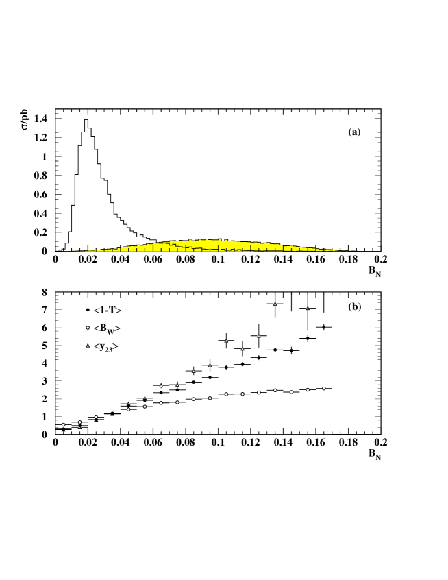
Figure 3: (a) Distributions (at 175 GeV) of $B_{N}$ for $\mbox{${\mathrm{Z}^{0}}$}/\gamma\rightarrow\mbox{$\mathrm{q\overline{q}}$}$ events having less than 1 GeV initial state radiation (open histogram) and for $\mathrm{W^{+}W^{-}}$$\rightarrow$$\mathrm{q\overline{q}}$$\mathrm{q\overline{q}}$ events (shaded) (b) average values of $(1-T)$, $B_{W}$ and $y_{23}^{(D)}$ (scaled by their overall mean values) as a function of $B_{N}$

In order to judge the correlation between $B_{N}$ and the observables which we would wish to use for the determination of $\alpha_{\mathrm{s}}$  we show in Fig. 3(b) the average values of $(1-T)$, $B_{W}$ and $y_{23}^{(D)}$ (normalized to their overall mean values) for non-radiative $\mbox{${\mathrm{Z}^{0}}$}/\gamma\rightarrow\mbox{$\mathrm{q\overline{q}}$}$ events as a function of $B_{N}$. It is evident that the $\mathrm{W^{+}W^{-}}$$\rightarrow$$\mathrm{q\overline{q}}$$\mathrm{q\overline{q}}$ contribution can be reduced to almost any level desired by cutting on $B_{N}$, but at an increasing cost in bias, and a corresponding loss in statistics. Generally, $M_{L}$ and $y_{34}^{(D)}$ show similar behaviour to $B_{N}$. The $D^{2}$ variable offers a less clean separation between the $\mbox{${\mathrm{Z}^{0}}$}/\gamma\rightarrow\mbox{$\mathrm{q\overline{q}}$}$ and $\mathrm{W^{+}W^{-}}$$\rightarrow$$\mathrm{q\overline{q}}$$\mathrm{q\overline{q}}$ events, but it appears that it may introduce somewhat less, or different, bias, and may thus be complementary.

These observations may be quantified in table 2 below, where we show the effect of various possible stage II cuts on the $\mbox{${\mathrm{Z}^{0}}$}/\gamma\rightarrow\mbox{$\mathrm{q\overline{q}}$}$ non-radiative signal and the $\mathrm{W^{+}W^{-}}$$\rightarrow$$\mathrm{q\overline{q}}$$\mathrm{q\overline{q}}$ background.
We give the average values of $1-T$, $B_{W}$ and $y_{23}^{(D)}$ as an indication of the bias caused by the cuts.

	$\mbox{${\mathrm{Z}^{0}}$}/\gamma\rightarrow\mbox{$\mathrm{q\overline{q}}$}$($E_{isr}<1$ GeV)				$\mathrm{W^{+}W^{-}}$$\rightarrow$$\mathrm{q\overline{q}}$$\mathrm{q\overline{q}}$
Cut(s)	$\sigma$ /pb	$<1-T>$	$<B_{W}>$	$<y_{23}^{(D)}>$	$\sigma$ /pb
$|\mbox{$\cos\theta$}_{T}|<0.9$	17.90	0.0598	0.0708	0.0196	6.08
Stage I only	16.51	0.0587	0.0701	0.0195	5.74
$B_{N}<$0.07	15.73	0.0528	0.0668	0.0169	1.34
$B_{N}<$0.06	15.27	0.0504	0.0653	0.0160	0.87
$B_{N}<$0.05	14.53	0.0474	0.0632	0.0149	0.50
$B_{N}<$0.04	13.26	0.0433	0.0601	0.0133	0.24
$M_{L}<$0.175	15.26	0.0504	0.0656	0.0161	1.37
$y_{34}^{(D)}<$0.0065	15.34	0.0501	0.0644	0.0156	0.88
$D^{2}>$300 GeV2	14.17	0.0543	0.0667	0.0164	1.90
$D^{2}>$600 GeV2	12.25	0.0504	0.0638	0.0140	0.89
$D^{2}>$600 GeV2 and $B_{N}<$0.06	11.71	0.0460	0.0613	0.0124	0.24
$D^{2}>$300 GeV2 and $B_{N}<$0.05	12.79	0.0457	0.0615	0.0132	0.24
$B_{N}-\sqrt{D^{2}}/2000<0.03$	13.84	0.0451	0.0612	0.0137	0.25

Table 2: Cross-sections at 175 GeV accepted after the Stage I cuts, and after various possible Stage II cuts. The average values of various relevant observables are also shown, to indicate the level of bias introduced.

We note that the stage I cuts cause only a small bias. We show several possible cuts on the $B_{N}$ variable. The background from $\mathrm{W^{+}W^{-}}$$\rightarrow$$\mathrm{q\overline{q}}$$\mathrm{q\overline{q}}$ may be reduced, for example, to a level of 4% with an efficiency for selection $\mbox{${\mathrm{Z}^{0}}$}/\gamma\rightarrow\mbox{$\mathrm{q\overline{q}}$}$ events of 82%. However, the sample of $\mbox{${\mathrm{Z}^{0}}$}/\gamma\rightarrow\mbox{$\mathrm{q\overline{q}}$}$ events accepted is strongly biased. The bias, as measured by the mean value of the observable, tends to be greatest for $y_{23}^{(D)}$ and smallest for $B_{W}$. We show similar results for cuts on $M_{L}$ and $y_{34}^{(D)}$, where we have chosen cuts which yield roughly the same $\mbox{${\mathrm{Z}^{0}}$}/\gamma\rightarrow\mbox{$\mathrm{q\overline{q}}$}$ efficiency as the $B_{N}<0.06$ cut. Cutting on $M_{L}$ is less effective than $B_{N}$ at removing $\mathrm{W^{+}W^{-}}$$\rightarrow$$\mathrm{q\overline{q}}$$\mathrm{q\overline{q}}$ background, while a cut on $y_{34}^{(D)}$ gives essentially the same performance as $B_{N}$. The cut on $D^{2}>600$ GeV² yields the same $\mathrm{W^{+}W^{-}}$$\rightarrow$$\mathrm{q\overline{q}}$$\mathrm{q\overline{q}}$ contamination (7%) as the $B_{N}<0.06$ cut, but for a significantly lower $\mbox{${\mathrm{Z}^{0}}$}/\gamma\rightarrow\mbox{$\mathrm{q\overline{q}}$}$ efficiency (69% compared to 85%). Using $D^{2}$ yields a somewhat smaller bias on $1-T$, but the bias on $y_{23}^{(D)}$ is a little greater. The two observables $B_{N}$ and $D^{2}$ are not strongly correlated (whereas, for example, $B_{N}$ and $M_{L}$ are highly correlated), suggesting that a joint cut on the two variables could give better separation. Examples are given in Table 2. The $\mathrm{W^{+}W^{-}}$$\rightarrow$$\mathrm{q\overline{q}}$$\mathrm{q\overline{q}}$ background may, for example, be reduced to around the 2% level for a $\mbox{${\mathrm{Z}^{0}}$}/\gamma\rightarrow\mbox{$\mathrm{q\overline{q}}$}$ efficiency of almost 80%, with somewhat less bias than a cut on $B_{N}$ alone. The precise cuts chosen for the separation of $\mbox{${\mathrm{Z}^{0}}$}/\gamma\rightarrow\mbox{$\mathrm{q\overline{q}}$}$ and $\mathrm{W^{+}W^{-}}$$\rightarrow$$\mathrm{q\overline{q}}$$\mathrm{q\overline{q}}$ events may therefore need to depend on the analysis being performed – whether a high purity is demanded, or whether a comparatively unbiased sample is required.

In Fig. 4(a) we show the distributions of a typical observable which may be used for the determination of $\alpha_{\mathrm{s}}$, $(1-T)$, after the stage I cuts. We compare the $\mbox{${\mathrm{Z}^{0}}$}/\gamma\rightarrow\mbox{$\mathrm{q\overline{q}}$}$ non-radiative ($E_{isr}<1$ GeV) signal with the $\mathrm{W^{+}W^{-}}$$\rightarrow$$\mathrm{q\overline{q}}$$\mathrm{q\overline{q}}$ background. In Fig. 4(b) we show the same distributions after the stage II cuts, taking $B_{N}<0.05$ as a typical stage II cut.

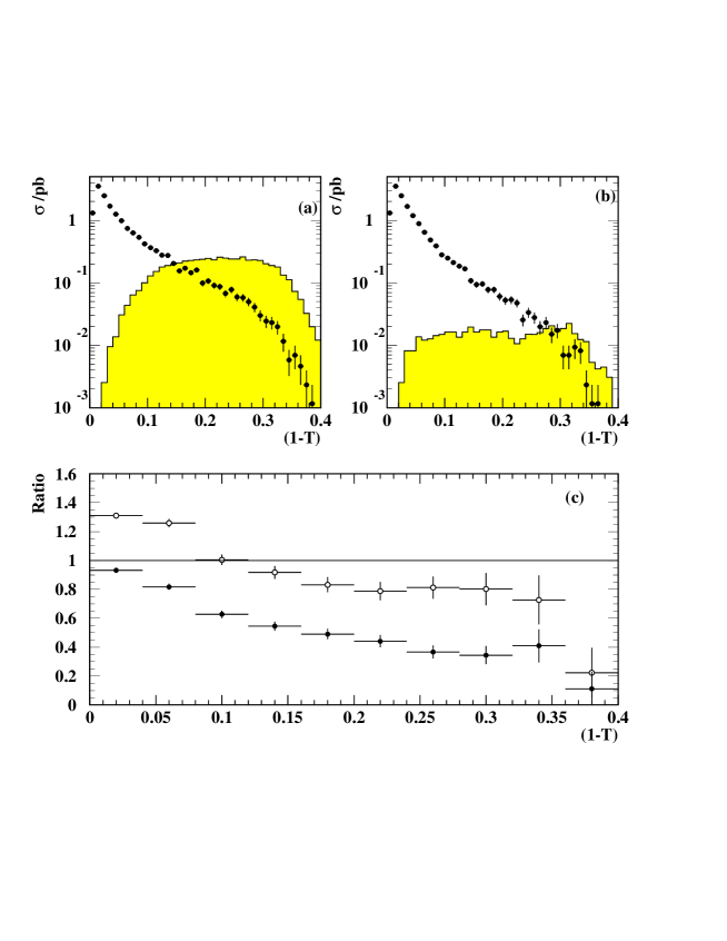
Figure 4: (a) Distributions (at 175 GeV) of $(1-T)$ after the stage I cuts. $\mbox{${\mathrm{Z}^{0}}$}/\gamma\rightarrow\mbox{$\mathrm{q\overline{q}}$}$ non-radiative ($E_{isr}<1$ GeV) events are shown as points with errors, and $\mathrm{W^{+}W^{-}}$$\rightarrow$$\mathrm{q\overline{q}}$$\mathrm{q\overline{q}}$ events by the shaded histogram. (b) as (a), after applying the stage I cuts and the stage II cut $B_{N}<0.05$. (c) Biases to the distribution of $(1-T)$. The stage I cuts and the stage II cut $B_{N}<0.05$ are applied. The closed points show the fraction of $\mbox{${\mathrm{Z}^{0}}$}/\gamma\rightarrow\mbox{$\mathrm{q\overline{q}}$}$ non-radiative ($E_{isr}<1$ GeV) events accepted after cuts. The open points show the ratio of all accepted $\mbox{${\mathrm{Z}^{0}}$}/\gamma\rightarrow\mbox{$\mathrm{q\overline{q}}$}$ events after cuts to non-radiative ($E_{isr}<1$ GeV) $\mbox{${\mathrm{Z}^{0}}$}/\gamma\rightarrow\mbox{$\mathrm{q\overline{q}}$}$ events before cuts.

As expected, the background tends to be concentrated toward large values of $(1-T)$, i.e. the region of hard gluon emission in the $\mbox{${\mathrm{Z}^{0}}$}/\gamma\rightarrow\mbox{$\mathrm{q\overline{q}}$}$ reaction. The two-jet region of the $\mbox{${\mathrm{Z}^{0}}$}/\gamma\rightarrow\mbox{$\mathrm{q\overline{q}}$}$ process is relatively free of background. Other stage II cuts give similar results. In Fig. 4(c) we show the efficiency of the stage I+II cuts, taking $B_{N}<0.05$ as a typical stage II cut, as a function of the $(1-T)$, for $\mbox{${\mathrm{Z}^{0}}$}/\gamma\rightarrow\mbox{$\mathrm{q\overline{q}}$}$ non-radiative ($E_{isr}<1$ GeV) events (solid points). As expected, the cuts bias against large values of $(1-T)$. In Fig. 4(c) we also show as open points the ratio of the distributions of all accepted $\mbox{${\mathrm{Z}^{0}}$}/\gamma\rightarrow\mbox{$\mathrm{q\overline{q}}$}$ events (including radiative events) to those of the non-radiative events before selection cuts. In general the effect of initial state radiation is to bias the distribution towards higher values, but this is counteracted by the tendency of the cuts to reject events with high values of the observables. The net effect is that the distribution of the accepted radiative $\mbox{${\mathrm{Z}^{0}}$}/\gamma\rightarrow\mbox{$\mathrm{q\overline{q}}$}$ events is quite similar to the distribution of non-radiative events before cuts, and so the ratios in Fig. 4(c) are increased roughly uniformly. Other stage II cuts give similar results, though the efficiencies may be systematically higher or lower.

2.3 Determination of $\alpha_{\mathrm{s}}$

Before comparing with QCD calculations, the observed data must be corrected for the effects of detector resolution, the acceptance of selection cuts and the effects of background (Fig. 4). The influence of hadronization must then be accounted for, and one standard way of doing this is to multiply the corrected hadron level data by the ratio of the parton level to hadron level distributions from a Monte Carlo model. In Fig. 5 we show these ratios for $(1-T)$, based on Jetset7.4, at 175 GeV (LEP2) and 91.2 GeV (LEP1).

Figure 5: Hadronization corrections for the distributions of $(1-T)$.

We note that the correction factors at LEP2 are significantly closer to unity, especially at small values of $(1-T)$, corresponding to the two-jet region. Similar comments apply to the other observables. A requirement for a credible analysis is that the correction factors be not too far from unity.

In this study, we investigate three types of QCD calculations, which may be used as the basis of a measurement of $\alpha_{\mathrm{s}}$ from event shape variables. These are:

${\cal O}(\alpha_{\mathrm{s}}^{2}$)

The QCD matrix elements, expanded as a power series in $\alpha_{\mathrm{s}}$ are fully known to ${\cal O}(\alpha_{\mathrm{s}}^{2}$) [17]. From previous studies at LEP1 we know that these calculations are applicable in the “3-jet” region, i.e. the region dominated by hard gluon radiation. A significant uncertainty in applying the ${\cal O}(\alpha_{\mathrm{s}}^{2}$) calculations is the choice of renormalization scale, $\mu$, represented by $\mbox{$x_{\mu}$}=\mu/E_{c.m.}$. The region over which the data can successfully be fitted can be extended further into the 2-jet region by choosing a small value of $\mbox{$x_{\mu}$}\sim 0.1$ (typically).

NLLA

In the 2-jet region, the expansion in powers of $\alpha_{\mathrm{s}}$ is bound to fail, because large logarithms arise associated with collinear and soft gluon emission. In this region, ”NLLA” calculations are available which resum the leading and next to leading logarithms to all orders in $\alpha_{\mathrm{s}}$. It has been shown in ref. [8] that such calculations may be used to derive $\alpha_{\mathrm{s}}$ at LEP1, but that it is necessary also to include a sub-leading term of the form $G_{21}\mbox{$\alpha_{\mathrm{s}}$}^{2}L$ in order to achieve a good description of the data.

Combined NLLA+${\cal O}(\alpha_{\mathrm{s}}^{2}$)

The most complete embodiment of our present knowledge of QCD comes from combining the ${\cal O}(\alpha_{\mathrm{s}}^{2}$) and NLLA calculations. It is necessary to match the calculations in such a way as to eliminate double counting of terms, and there are several ways of doing this. These have been studied at LEP1, based on which we choose the “$\ln R$” matching scheme for the present work.

To assess the range of validity of these calculations at LEP2 we proceed in the following empirical manner. We have generated distributions of the five observables, $(1-T)$, $M_{H}$, $B_{T}$, $B_{W}$ and $y_{23}^{(D)}$, at the parton level, using the Jetset7.4 parton shower model without initial state radiation. We can assume that the data, after correction for detector acceptance, the effect of selection cuts and background, and hadronization, would closely resemble these distributions. For each observable, we then determine the largest range for which the theoretical calculations reproduce those from Jetsetwith an acceptable $\chi^{2}/{\bf DOF}$. The results are summarised in Table 3. We note that the ${\cal O}(\alpha_{\mathrm{s}}^{2}$) calculations may (in most cases) be extended to lower values of the observables by fitting $x_{\mu}$. The NLLA or combined calculations allow a description down to still lower values, but, particularly in the case of the pure NLLA calculations, the higher values of the observables are less well modelled. The NLLA and combined calculations for $B_{W}$ tend to give a rather poor description of the Jetset “data” (as seen at LEP1). The pure NLLA calculations are not applied to $y_{23}^{(D)}$, since they are known to be incomplete, and in fact yield a poor fit to the Jetset distributions.

Observable	${\cal O}(\alpha_{\mathrm{s}}^{2}$) ($x_{\mu}$=1)	${\cal O}(\alpha_{\mathrm{s}}^{2}$) ($x_{\mu}$ fitted)	pure NLLA	Combined ${\cal O}(\alpha_{\mathrm{s}}^{2}$)+NLLA
$(1-T)$	0.09–0.3	0.05–0.3	0.02–0.17	0.02–0.3
$M_{H}$	0.20–0.55	0.14–0.55	0.10–0.35	0.14–0.55
$B_{T}$	0.11–0.3	0.10–0.3	0.05–0.18	0.05–0.22
$B_{W}$	0.06–0.26	0.06–0.26	0.02–0.12	0.05–0.17
$y_{23}^{(D)}$	0.015–0.2	0.005–0.2	–	0.005–0.2

Table 3: Approximate ranges of applicability of various types of QCD calculation.

If, for example, we require that the hadronization corrections lie between 0.8 and 1.2, that the $\mbox{${\mathrm{Z}^{0}}$}/\gamma\rightarrow\mbox{$\mathrm{q\overline{q}}$}$ acceptance be greater than 50% and that the $\mathrm{W^{+}W^{-}}$$\rightarrow$$\mathrm{q\overline{q}}$$\mathrm{q\overline{q}}$ contamination be less than 50%, the regions where the data can be used reliably would be roughly 0.03–0.2 for $(1-T)$, 0.15–0.4 for $M_{H}$, 0.06–0.2 for $B_{T}$, 0.03–0.18 for $B_{W}$ and 0.005–0.09 for $y_{23}^{(D)}$. By comparison with Table 3 it is evident that the regions in which reliable data may be obtained are best matched by the regions in which the combined NLLA+${\cal O}(\alpha_{\mathrm{s}}^{2}$) calculations are valid. Since these are also the most complete calculations, this would appear to be the most promising approach.

We next assess the precision on $\alpha_{\mathrm{s}}$ which could be achieved using 500 pb^-1 of data at LEP2. In order to do this, we take the Jetset7.4 parton level distribution, with statistical errors corresponding to this integrated luminosity (approximately 6500 $\mbox{${\mathrm{Z}^{0}}$}/\gamma\rightarrow\mbox{$\mathrm{q\overline{q}}$}$ events). We then fit the QCD theory to infer $\alpha_{\mathrm{s}}$, fitting in the range of the observable given by the overlap of the ranges in Tables 3 and the regions where reliable data may be obtained. A typical fit (of the ${\cal O}(\alpha_{\mathrm{s}}^{2}$)+NLLA calculations to $(1-T)$) is shown in Fig. 6.

Figure 6: Typical fit of the${\cal O}(\alpha_{\mathrm{s}}^{2}$)+NLLA QCD calculations to $(1-T)$ in order to determine $\alpha_{\mathrm{s}}$. The dotted lines delimit the fit region.

We find that the ${\cal O}(\alpha_{\mathrm{s}}^{2}$) calculations yield typical statistical errors of $\pm 0.0024$, which are larger than the NLLA and combined ${\cal O}(\alpha_{\mathrm{s}}^{2}$)+NLLA calculations (typically $\pm 0.0015$) because the former are only applicable towards the 3-jet region, where the few events are found. It also appears that the statistics are generally insufficient to permit a precise determination of the scale factor $x_{\mu}$ for the ${\cal O}(\alpha_{\mathrm{s}}^{2}$) fits. The pure NLLA and combined ${\cal O}(\alpha_{\mathrm{s}}^{2}$)+NLLA calculations both appear to be competitive, and offer the possibility of measuring $\alpha_{\mathrm{s}}$ with a statistical precision of around $\pm 0.0015$. For the event shapes $(1-T)$, $M_{H}$, $B_{T}$ and $B_{W}$, the NLLA tend to yield smaller values of $\alpha_{\mathrm{s}}$, and the ${\cal O}(\alpha_{\mathrm{s}}^{2}$) calculations larger values; the same trend was noted at LEP1 [8].

As at LEP1, the combined ${\cal O}(\alpha_{\mathrm{s}}^{2}$)+NLLA method will probably be the preferred technique, because it represents the most complete theoretical calculations, and allows the largest fraction of the data to be included in the analysis. For the discussion of possible systematic uncertainties, we therefore focus on these calculations. In ref. [7], for example, a wide range of systematic effects were investigated. The largest contribution was found to arise from variation of the renormalization scale factor $x_{\mu}$. Other significant effects arose from varying the hadronization model, particularly from the use of the Herwig model, and from the influence of b-quark mass effects. We have estimated the systematic errors resulting from these effects at 175 GeV, and compared with the LEP1 experimental results.

• The renormalization scale factor is varied in the range 0.5$<\mbox{$x_{\mu}$}<$2.0. The changes in $\alpha_{\mathrm{s}}$ are highly correlated with those at LEP1, though about 20% smaller on average. If we assume that it makes sense to choose the same scale factor at LEP2 as at LEP1, then the effective systematic uncertainty on the change in $\alpha_{\mathrm{s}}$ between LEP1 and LEP2 would be about $\pm 0.0015$ for $(1-T)$, $\pm 0.0025$ for $M_{H}$, $\pm 0.0015$ for $B_{T}$, $\pm 0.0005$ for $B_{W}$ and $\pm 0.0003$ for $y_{23}^{(D)}$.

• The influence of b-quark mass effects may be crudely accounted for by basing the parton level distributions in the correction procedure only on udsc quark events. At LEP1 this correction was found to increase $\alpha_{\mathrm{s}}$ by about 0.002 for most observables. Not surprisingly, the effect is much smaller at LEP2. However, the relevant point is the difference between the LEP1 and LEP2 uncertainties, which is of the order of 0.002 (somewhat larger for $B_{T}$ and smaller for $M_{H}$).

• The Herwig model offers a quite different hadronization scheme from Jetset. Since the hadronization corrections are smaller at LEP2 than at LEP1, we would expect the uncertainty associated with the use of different models to be reduced. This is generally the case, but the correlation between the Herwig uncertainties at LEP1 and LEP2 is unclear. This is partly because different fit regions have been used, and also different versions of the models. Clearly, in order to establish a reliable systematic uncertainty on the difference in $\alpha_{\mathrm{s}}$ between LEP1 and LEP2 it would be necessary to make a more careful analysis using consistent versions of the models at the two energies. For some observables at least (e.g. $B_{W}$ and $y_{23}^{(D)}$) it seems plausible that the hadronization uncertainty could be quite small.

In summary, it appears that systematic errors would not preclude making a useful measurement of the difference in $\alpha_{\mathrm{s}}$ between LEP1 and LEP2. The renormalization scale uncertainty seems to be comparable with or smaller than the statistical error. The uncertainty associated with b-quark mass effects could perhaps be reduced by further analysis and theoretical work. The uncertainties associated with the choice of hadronization models are less clear; it may be necessary to reanalyse the LEP1 data using the same models and parameter sets as employed in the LEP2 analysis, and the same fit regions, in order to minimise the uncertainties. Nonetheless, it seems that the systematic errors could be quite small, for some observables at least (especially $B_{W}$ and $y_{23}^{(D)}$, according to our study). It may be noted that recent studies of non-perturbative (power) corrections to the mean values of event shape observables [18] suggest that certain observables or combinations of observables might be expected theoretically to have especially small hadronization uncertainties (e.g. $y_{23}^{(D)}$ or $T-2C/3\pi$ [19]).

3 Event Shapes – Theoretical

Since the completion of the Yellow Report for LEP1 [20] much progress has been achieved in the theoretical calculations of shape variable distributions. A technique of resummation of contributions enhanced near the two–jet region has been studied and fully implemented in refs. [22, 11, jp_CDOTW, 23, 24, 25, 26, 27, 28, 29, 30, 31]. Furthermore, new calculations of shape variable distributions (implemented as computer code) have become available.

Calculation of shape variables are all based upon the original work of ref. [ERT]. This calculation was also performed in ref. [21]. Although the analytic results did agree, several problems where found in the comparison of numerical results (see ref. [20] for a small review). While at the time of ref. [20] it was hard to find precision calculations of jet shape distributions that agreed with each other, today we have at least three general purpose programs that do agree. One, the program EVENT, was developed for ref. [20]. Results of shape variables distributions performed with this program are reported there, and have served as a benchmark for comparison with other computations. In ref. [36] a new computation was performed, which agrees with good accuracy with ref. [20]. Furthermore, very recently, yet another calculation was completed [37]. In ref. [37] also oriented events are implemented, and apparently they will also be implemented in ref. [36]. This means that it will be possible to compute distribution of shape variables that do depend upon the orientation of the incoming beams axis, unlike all shape variables that where used up to now (see the next section).

The most disturbing disagreement on shape variables was found to be on the Energy-Energy correlation (EEC). The computation performed in ref. [34] was found in important disagreement with other calculations, and in particular with ref. [20]. Recently, in ref. [35] the calculation of ref. [34] was repeated. The result of the new calculation was found in disagreement both with the result of ref. [20] and with ref. [34]. No clear statement is made in ref. [35] upon the origin of the discrepancy. It is however claimed that the disagreement comes from the region in which besides the quark–antiquark pair, two soft gluons have been radiated. The EEC is in fact peculiar, in the sense that even configurations with thrust near 1 can contribute to the EEC at angles far away from $0$ and $\pi$. Because of the lack of a more complete theoretical paper form the authors of ref.  [35], we thought that the most useful thing to be done for the present report is to perform a high–precision comparison of the different computations of the EEC, that can serve as benchmark for future calculations. In order to achieve high precision, instead of computing the EEC itself as a function of the angle, we computed its moments. The energy-energy correlation is defined as

$$\mbox{EEC}(\chi)=\frac{1}{\sigma}\sum_{ij}\;\int d^{3}\vec{p}_{i}\,d^{3}\vec{p}_{j}\;\frac{d\sigma}{d^{3}\vec{p}_{i}\,d^{3}\vec{p}_{j}}\frac{E_{i}\,E_{j}}{E^{2}}\;\delta(\vec{p}_{i}\cdot\vec{p}_{j}-\cos\chi)\;.$$ (1)

We define

$$\int\mbox{EEC}(\chi)\;\sin^{2+m}\chi\;\cos^{n}\chi\;d\cos\chi=\frac{\mbox{$\alpha_{\mathrm{s}}$}}{2\pi}A_{\rm EEC}^{(m,n)}+\left(\frac{\mbox{$\alpha_{\mathrm{s}}$}}{2\pi}\right)^{2}B_{\rm EEC}^{(m,n)}+{\cal O}(\mbox{$\alpha_{\mathrm{s}}$}^{3})$$ (2)

where $\mbox{$\alpha_{\mathrm{s}}$}=\mbox{$\alpha_{\mathrm{s}}$}(E_{\rm cm})$. The coefficients $B_{\rm EEC}^{(m,n)}$ have the following colour structure

$$B_{\rm EEC}^{(m,n)}=C_{F}\left(C_{A}\,B_{C_{A}}^{(m,n)}+C_{F}\,B_{C_{F}}^{(m,n)}+T_{f}\,n_{f}\,B_{T_{f}}^{(m,n)}\right).$$ (3)

We then asked K. Clay (C), N. Glover (G), M. Seymour (S), and the author (N), to compute $B_{C_{A}}^{(m,n)}$, $B_{C_{F}}^{(m,n)}$, $B_{T_{F}}^{(m,n)}$ with the programs of ref. [35], [36], [37] and [20] for $m=0,\ldots,5$ and $n=0,1$. All four computations agreed within errors for the $B_{T_{F}}^{(m,n)}$ term. In the other two cases we found disagreements. The results are reported in tables 4 and 5.

m	n	N	G	S	C
0	0	$50.82\pm 0.05$	$50.54\pm 0.03$	$50.72\pm 0.02$	$46.4\pm 0.2$
1	0	$35.76\pm 0.04$	$35.53\pm 0.02$	$35.64\pm 0.02$	$32.09\pm 0.06$
2	0	$28.94\pm 0.03$	$28.75\pm 0.02$	$28.82\pm 0.02$	$25.73\pm 0.04$
3	0	$24.92\pm 0.03$	$24.75\pm 0.02$	$24.80\pm 0.02$	$22.03\pm 0.04$
4	0	$22.20\pm 0.03$	$22.05\pm 0.02$	$22.09\pm 0.02$	$19.54\pm 0.04$
5	0	$20.21\pm 0.03$	$20.07\pm 0.02$	$20.10\pm 0.02$	$17.74\pm 0.03$
0	1	$-6.468\pm 0.006$	$-6.50\pm 0.01$	$-6.455\pm 0.005$	$-6.0\pm 0.15$
1	1	$-2.356\pm 0.004$	$-2.365\pm 0.009$	$-2.344\pm 0.003$	$-2.15\pm 0.03$
2	1	$-1.189\pm 0.003$	$-1.194\pm 0.008$	$-1.177\pm 0.003$	$-1.06\pm 0.02$
3	1	$-0.714\pm 0.003$	$-0.718\pm 0.007$	$-0.702\pm 0.003$	$-0.62\pm 0.01$
4	1	$-0.478\pm 0.003$	$-0.479\pm 0.007$	$-0.466\pm 0.003$	$-0.41\pm 0.01$
5	1	$-0.344\pm 0.003$	$-0.344\pm 0.006$	$-0.331\pm 0.003$	$-0.28\pm 0.01$

Table 4: Comparison of different computations of the $B_{C_{A}}^{(m,n)}$ coefficients.

m	n	N	G	S	C
0	0	$-13.29\pm 0.01$	$-13.94\pm 0.05$	$-13.40\pm 0.05$	$7.2\pm 0.2$
1	0	$-5.09\pm 0.01$	$-5.38\pm 0.04$	$-5.14\pm 0.04$	$9.98\pm 0.04$
2	0	$-2.98\pm 0.01$	$-3.20\pm 0.03$	$-3.02\pm 0.03$	$9.55\pm 0.03$
3	0	$-2.11\pm 0.01$	$-2.29\pm 0.03$	$-2.14\pm 0.03$	$8.86\pm 0.02$
4	0	$-1.65\pm 0.01$	$-1.81\pm 0.03$	$-1.67\pm 0.03$	$8.22\pm 0.02$
5	0	$-1.36\pm 0.01$	$-1.51\pm 0.03$	$-1.39\pm 0.03$	$7.69\pm 0.02$
0	1	$4.906\pm 0.002$	$4.92\pm 0.01$	$4.892\pm 0.006$	$2.6\pm 0.2$
1	1	$0.240\pm 0.002$	$0.259\pm 0.008$	$0.232\pm 0.004$	$-0.58\pm 0.02$
2	1	$-0.383\pm 0.002$	$-0.367\pm 0.006$	$-0.386\pm 0.004$	$-0.80\pm 0.01$
3	1	$-0.458\pm 0.002$	$-0.445\pm 0.005$	$-0.459\pm 0.003$	$-0.72\pm 0.01$
4	1	$-0.428\pm 0.002$	$-0.417\pm 0.005$	$-0.429\pm 0.003$	$-0.606\pm 0.007$
5	1	$-0.381\pm 0.002$	$-0.371\pm 0.004$	$-0.381\pm 0.003$	$-0.510\pm 0.006$

Table 5: Comparison of different computations of the $B_{C_{F}}^{(m,n)}$ coefficients.

It is clear that the results N, G and S agree with each other with high accuracy, while C is seriously different. Observe that, although for all practical purposes N, G and S agree with each other, there are among them discrepancies of several standard deviations. We attributed these differences as an underestimate of the errors, rather than to a real difference in the calculation. More details on the different characteristics of the three computer codes are given in the generator’s section [38].

4 Next-to-leading Order Calculations of Oriented Event Shapes

At LEP2, it will become increasingly important to be able to cut out some angular regions to control the backgrounds, and to define event shapes that are invariant under boosts along the beam direction to study continuum events with initial-state radiation. To make predictions for such quantities it is essential to use the full matrix elements for $\mathrm{e^{+}e^{-}\to q\bar{q}g},$ including the full Z$/\gamma$ interference and the polarisation of the exchanged boson. Two programs have recently become available that include these matrix elements, EERAD[39] and EVENT2[MHScs]. These use completely different methods to implement the cancellation of poles between real and virtual contributions, as described in [38], but the results are in excellent agreement with each other.

As an example of an oriented event shape we study the thrust distribution as a function of the thrust axis direction. As usual[MHSlep1], we parametrize the distribution as

$$\frac{1}{\sigma_{0}}(1-T)\frac{d\sigma}{dTd\!\cos\theta}=\frac{\alpha_{s}(\mu^{2})}{2\pi}A(T,\cos\theta)+\left(\frac{\alpha_{s}(\mu^{2})}{2\pi}\right)^{2}\left[A(T,\cos\theta)2\pi b_{0}\log\frac{\mu^{2}}{s}+B(T,\cos\theta)\right]\!.$$ (4)

The definition of thrust has a forward-backward ambiguity, so we are at liberty to define $\cos\theta>0$. The leading order term is known analytically[40],

$$A(T,\cos\theta) = C_{F}\left[\left\{\frac{2(3T^{2}-3T+2)}{T}\log\frac{2T-1}{1-T}-3(3T-2)(2-T)\right\}\mbox{$\frac{3}{4}$}(1+\cos^{2}\theta)\right.$$ (5)

$$\phantom{C_{F}}\;\;\left.+\left\{\frac{2(3T-2)(2-T)(1-T)}{T^{2}}\right\}\mbox{$\frac{3}{4}$}(1-3\cos^{2}\theta)\right].$$

Integration over $\cos\theta$ immediately gives us the expression in [MHSlep1]. Numerical results for $A$ and $B$ are shown in Fig. 7.

Figure 7: The coefficients of the thrust distribution for five bins in $\cos\theta,$ where $\theta$ is the angle between the thrust axis and the beam. The errors shown are purely statistical and are similar for each histogram, so we only show them for one.

Combining these coefficients with an $\alpha_{s}$ value and factorisation scale choice, $\alpha_{s}(\mu^{2}=s)=0.120,$ we obtain the predictions shown in Fig. 8a.

Figure 8: Predictions for the thrust distribution for five bins in $\cos\theta$ normalized to (a) the total number of events and (b) the number of events in each bin.

Alternatively, we can divide out the trivial dependence on $\cos\theta$ by normalising each curve to the number of events in that bin, given by[40]

$$\frac{1}{\sigma_{0}}\frac{d\sigma}{d\!\cos\theta}=\mbox{$\frac{3}{4}$}(1+\cos^{2}\theta)\left\{1+\frac{\alpha_{s}}{\pi}\right\}+\frac{\alpha_{s}}{\pi}\left\{8\log\frac{3}{2}-3\right\}(1-3\cos^{2}\theta)\approx\mbox{$\frac{3}{4}$}(1+\cos^{2}\theta)+\frac{\alpha_{s}}{\pi},$$ (6)

where the approximation is good to better than 1%. The result is shown in Fig. 8b, where we see that the majority of the $\cos\theta$ dependence in Fig. 8a was from this dependence of the total event rate and the residual dependence is rather small. Nevertheless, it should be measurable with the full statistics of LEP1.

5 Fragmentation functions

The measurement of fragmentation functions at different energies and the comparison with the theoretical predictions, either implemented in the Monte Carlo programs or deduced from other measured data, can be used to perform different QCD tests and to tune the parameters describing the fragmentation processes inside the Monte Carlo programs.

At the energies available at LEP II the scaled energy ($x\equiv 2E/\sqrt{s}$) distributions for charged particles can be measured for ${\mathrm{q}}\overline{\mathrm{q}}$ events in which the mass of the hadronic system is close to the centre–of–mass energy of the collision. Furthermore, the fragmentation function of the W boson can also be measured and compared to the expectation that comes from the measurement of the fragmentation functions for different enriched flavour samples at LEP I, after correcting for the small scaling produced for the different masses of the Z and the W boson and for the different flavour composition.

This Section describes how the measurement of the scaled energy distributions can be made and what can be expected in the measurement of $\alpha_{s}$ from scaling violations.

5.1 Measurement of scaled energy distributions

The measurement of the charged scaled energy distributions will follow the same procedure used at lower centre–of–mass energies. At centre–of–mass energies of the Z mass, hadronic events can be selected with very high purity and small backgrounds (coming mainly from $\tau$ events). At LEP II centre–of–mass energies, most of the $q\bar{q}$ events (more than 75%) will radiate an initial state hard photon such a way that the effective centre–of–mass energy of the collision will be reduced to below 120 GeV. These events have a high boost along the collision axis and have to be removed.

The selection of hadronic events will follow a procedure very similar to the one presented in subsection 2.2. After some minimal requirements on track quality, number of tracks and total measured energy of these tracks, additional selection variables have to be considered. Good containment of the events can be obtained with cuts in the sphericity or thrust axis.

Monte Carlo simulations performed in ALEPH, based upon DYMU3 and JETSET, including full simulation of the detector response, show that requiring a visible mass of the event above 120 GeV and a normalized balanced momentum of the charged tracks along the beam axis below 0.3, a selection efficiency of $\sim 18\%$ can be achieved. The percentage of selected events such that the invariant mass of the propagator is below 120 GeV is reduced to approximately 7% with this selection procedure.

The backgrounds from dilepton events are small at this level. However, the background from WW events could still be substantial. A cut in missing momentum will remove most of the events in which one of the W has decayed leptonically. The remaining events in which both W decay hadronically can be removed by considering appropriate shape variables. Events resulting from the fragmentation of two W bosons will have a four-jet topology that makes them more spherical than the ones resulting from $\mathrm{Z}/\gamma\rightarrow{\mathrm{q}}\overline{\mathrm{q}}$. In subsection 2.2 a discussion of the various possible approaches is given. For the case of the measurement of the scaled energy distributions, a cut on thrust $T>0.925$ would be appropriate, since (unlike the case of shape variables) such a cut does not introduce strong biases in the shape of the fragmentation function.

The whole selection procedure should result in a cross section for ${\mathrm{q}}\overline{\mathrm{q}}$ events of $~{}\sim 11$ pb with less than 1% of events with the effective centre–of–mass energy below 120 GeV and with a background of WW events below 5%. Assuming an integrated luminosity of 500 pb^-1 the expectation is to have $\sim 6000$ selected hadronic events.

It can be assumed that the background can be subtracted statistically using Monte Carlo techniques, and that the distribution is corrected using a hadronic event generator (with parameters adjusted to describe the data) for the effects of geometrical acceptance, detector efficiency and resolution, decays of long-lived particles (with $\tau>1$ ns), secondary interactions and residual initial state photon radiation. The bin-to-bin correction factors are below 10% using the selection described above.

Figure 9: Scaled energy distribution for hadronic events at a centre–of–mass energy of 180 GeV according to the JETSET Monte Carlo. The error bars correspond to the statistics of 6000 events.

Figure 9 shows the Monte Carlo scaled energy distribution for the statistics of 6000 events. The energies of the particles before detector effects have been used to construct the distribution. Additional systematic uncertainties coming from possible discrepancies between the real detector performance and the simulated one and from the dependence on the hadron production model used to correct the data for detector effects will have to be considered.

The measurement of the W fragmentation function will require the selection of hadronic W events. The events in which one of the W decays leptonically can be selected using missing momentum or tagging a high-momentum lepton. The rest of the particles can be used to determine the momentum of the hadronically decaying W boson and to construct the scaled energy distribution, after boosting the particles into the rest frame of the parent W boson. In the case that both W bosons decay hadronically the techniques used in the measurement of the W mass can be used to unambiguously assign the jets to the corresponding W bosons.

5.2 Scaling violations: QCD tests

The analysis of scaling violations with the data available at LEP and data from lower centre–of–mass energy experiments (PEP, PETRA, TRISTAN) has focused on the measurement of $\alpha_{s}$ [41, 42]. The prediction of scaling violations in fragmentation functions of quarks and gluons is similar to that predicted in structure functions in deep-inelastic lepton-nucleon scattering.

In an electron-positron collider, scaling violations are observed in the dependence of the distribution of the scaled energy of final-state particles in hadronic events on the centre–of–mass energy $\sqrt{s}$. This comes about because with increasing $\sqrt{s}$ more phase space for gluon radiation and thus for final-state particle production becomes available, leading to a softer $x$-distribution. As the probability for gluon radiation is proportional to the strong coupling constant, a measurement of the scaled-energy distributions at different centre–of–mass energies compared to the QCD prediction allows one to determine the only free parameter of QCD, $\alpha_{s}$. A recent review of the relevant theoretical ideas has been given in ref. [43]. For another recent theoretical analysis see [44].

A reliable measurement of scaling violations has to disentangle the true QCD evolution from effects due to the dependence of the flavour composition upon the centre–of–mass energy. Since heavy flavours, after their decay into light particles, typically have softer fragmentation functions, when going from centre–of–mass energies below the Z mass towards the Z mass, the $b$ content increases, and it decreases again when going towards higher energies. To analyse the data in a model independent way, final-state flavour identification and a measurement of the gluon fragmentation function are needed. This procedure has been followed in the analysis performed in ref. [41], where enriched $uds$-, $c$-, and $b$-quark scaled energy distributions, together with the measurement of the gluon fragmentation functions and the longitudinal cross section, have been used to constraint the fragmentation functions for the different flavours and the gluon. It was assumed that the fragmentation functions of $u$, $d$, and $s$ quarks are the same. In the analysis presented there, a total of 15 parameters besides $\alpha_{s}$ are fitted to all the available. The parameters contain information on the fragmentation functions for the different quarks and the gluon and also a parametrisation of the non-perturbative contributions to the evolution. The value of the strong coupling constant obtained from this fit is

$$\mbox{$\alpha_{s}(M_{Z})$}=0.126\pm 0.007(exp)\pm 0.006(theory)=0.126\pm 0.009{\mbox{\hskip 14.22636pt}}.$$ (7)

The experimental error is the result of the combination in quadrature of the errors from the fit (0.0053), the uncertainties in the flavour composition of the enriched scaled energy distributions and the assumptions on the normalisation errors for those low-energy experiments where this error is not specified. The theoretical error is estimated by varying the factorisation and renormalisation scales.

A possible extension of this analysis has been investigated by including the predicted distribution measured at a centre–of–mass energy of 180 GeV (figure 9). Figure 10 shows the result of the fit to the scaled energy distributions at three centre–of–mass energies (29 GeV, 91.2 GeV and 180 GeV). The fact that the variations with energy of the fragmentation functions is logarithmic makes the difference between the distributions at 180 GeV and 91.2 GeV smaller than that between 91.2 GeV and 29 GeV. This is accentuated by the fact that the flavour composition changes between 91.2 GeV and 180 GeV, in particular the percentage of $b$ quarks diminishes when going to energies above the Z pole. Since the fragmentation function for $b$ quarks is softer, this hardens the inclusive distribution at LEP II energies.

Figure 10: Result of the scaling violation fit to the distributions at centre–of–mass energies at 29 GeV, 91.2 GeV and 180 GeV.

The error in $\alpha_{s}(M_{Z})$ coming from the fit is not improved by including the distribution measured at 180 GeV. It was found, however, that with four times the predicted available statistics, a 10% improvement in this error could be obtained. The conclusion is that the analysis could serve as another consistency check of the predicted QCD scaling violations. Improvement in the error on $\alpha_{s}(M_{Z})$ may come from several sources. A better understanding of the flavour tagging algorithms used to measure the flavour-enriched distributions could improve the experimental systematic error. Progress on the theoretical side, for example the extension of the formalism to describe better the low–$x$ region (see Section 5.3) could also be helpful.

Another consistency check can be performed by using the measured flavour-enriched distributions at the Z peak and the scaling violation formalism to predict the fragmentation function in W decays. The fragmentation functions obtained from the fit to all data for the different quark flavours can be evolved to the mass of the W. Then the W scaled energy distribution can be predicted using the W decay branching ratios for each flavour. Figure 11 shows, in the continuous line, the prediction that results from this procedure. The points are the W scaled energy distribution as predicted by the PYTHIA Monte Carlo.

Figure 11: W fragmentation function predicted by the PYTHIA Monte Carlo (points), compared with the QCD prediction resulting from the analysis of scaling violations.

5.3 Small-$x$ fragmentation

In the region of small values of the momentum fraction $x$, the behaviour of the fragmentation functions may be significantly affected by phenomena related to the coherence of soft gluon radiation (for a review of this subject see, for instance, Ref. [46]). These effects are expected to result in a suppression of hadron production in the small-$x$ (or soft) region, and to modify both the $x$-shape and the $Q^{2}$-dependence of the inclusive single-particle spectrum. In particular, as a consequence of coherence, when the momentum fraction becomes small the gluon fragmentation function is expected to peak at a value dependent on the hard scale of the process, and be damped in the soft region.

From the standpoint of perturbation theory, coherence effects show up as logarithmic corrections $\alpha_{S}^{k}\log^{m}(1/x)$ ($m\leq 2k-2$) to the splitting and coefficient functions which control the perturbative evaluation of the fragmentation functions. For example, the gluon splitting function $P_{gg}(\alpha_{S},x)$ has the small-$x$ behaviour (${\bar{\alpha}}_{S}\equiv\alpha_{S}N_{c}/\pi$)

$$P_{gg}(\alpha_{S},x)\simeq{{\bar{\alpha}}_{S}\over x}-{{\bar{\alpha}}_{S}^{2}\over x}\log^{2}x+{{\bar{\alpha}}_{S}^{3}\over{3x}}\log^{4}x+\dots\;\;\;\;,\;\;x\ll 1\;\;.$$ (8)

Small-$x$ logarithms are present to all orders in $\alpha_{S}$, and a systematic way to take coherence effects into account is to resum these logarithms to the leading accuracy, next-to-leading accuracy, and so on.

The leading-log results were determined in Refs. [22, 47], and can be best given in the moment space defined via the Mellin-Fourier transform

$$\gamma_{gg}(\alpha_{S},\omega)\equiv\int_{0}^{1}dx\;x^{\omega}\;P_{gg}(\alpha_{S},x)\;\;\;\;,$$ (9)

and the analogous transform for any other function of $x$. In the moment space logarithmic terms appear as multiple poles at $\omega\to 0$, and the summation of the leading contributions ${\cal O}\left(\alpha_{S}^{k}/\omega^{2k-1}\right)$ is encompassed by the formula [48]

$$\gamma_{gg}(\alpha_{S},\omega)={1\over 4}\left(\sqrt{\omega^{2}+8\,{\bar{\alpha}}_{S}}-\omega\right)\;\;.$$ (10)

The perturbative behaviour of this formula can be obtained by expanding it in the coupling $\alpha_{S}$. The first terms of the expansion read as follows

$$\gamma_{gg}(\alpha_{S},\omega)\simeq{{\bar{\alpha}}_{S}\over\omega}-2{{\bar{\alpha}}_{S}^{2}\over{\omega^{3}}}+8{{\bar{\alpha}}_{S}^{3}\over{\omega^{5}}}+\dots\;\;\;\;\;\;,$$ (11)

where in the ${\cal O}(\alpha_{S})$ and ${\cal O}(\alpha_{S}^{2})$ terms one may recognize the dominant part at small $x$ of the standard one-loop and two-loop evolution kernels for the fragmentation functions (see [nw] and references therein), whilst higher-order terms represent corrections due to coherent emission of soft gluons. An important feature which can be observed in Eq. (11) is the alternating sign of the expansion. As a matter of fact, this feature extends to the whole series, and the net effect of resumming all the leading logarithms turns out to be a damping of the fragmentation function in the soft region with respect to the lowest-order prediction.

The asymptotic properties of the resummed expression (10) are conversely determined by its behaviour near $\omega=0$. This is given by

$$\gamma_{gg}(\alpha_{S},\omega)\sim\sqrt{{{\bar{\alpha}}_{S}\over 2}}\;\;\;\;,\;\;\omega\to 0\;\;\,.$$ (12)

Note that the all-order summation of the perturbative poles $\alpha_{S}^{k}/\omega^{2k-1}$ gives rise to a finite result at $\omega=0$, and introduces on the other hand the non-analytic behaviour in $\alpha_{S}$ of the square-root type.

The summation of the next-to-leading contributions ${\cal O}\left(\alpha_{S}^{k}/\omega^{2k-2}\right)$ has also been performed [49]. The explicit expression of the next-to-leading correction to Eq. (10) reads

$$\gamma_{gg}^{NL}(\alpha_{S},\omega) = \gamma_{gg}^{L}+{\bar{\alpha}}_{S}\left[-{{11}\over{12}}-{{N_{f}}\over{6\,C_{A}}}+\left({11\over 4}+{{N_{f}}\over{3\,C_{A}}}-{2\over 3}{{N_{f}\,C_{F}}\over{C_{A}^{2}}}\right)\,{{\gamma_{gg}^{L}}\over{4\,\gamma_{gg}^{L}+\omega}}\right.$$ (13)

$$- \left.{11\over 12}\,{{\omega\,\gamma_{gg}^{L}}\over{(4\,\gamma_{gg}^{L}+\omega)^{2}}}-{2\over 3}\,{{N_{f}}\over{C_{A}}}\,{{{\gamma_{gg}^{L}}^{2}}\over{(4\,\gamma_{gg}^{L}+\omega)^{2}}}\right]\;\;\;,$$

where $\gamma_{gg}^{L}$ denotes the leading term (10), and $N_{f}$ is the number of flavours. Next-to-leading contributions do not alter the qualitative behaviour determined by the leading-order analysis, but provide a ${\cal O}(\sqrt{\alpha_{S}})$ correction to the position of the peak in the gluon fragmentation function.

Phenomenological studies of the soft region of the single-particle spectrum have been carried out in Ref. [50], on the basis of modified evolution equations which hold in the small-$x$ regime. The central region of the spectrum, on the other hand, is known to be well described by second-order perturbation theory. It is therefore important to develop a procedure in which resummed contributions are consistently matched on to second-order perturbation theory, in order to get a uniform description of fragmentation over the whole phase space.

6 Charged Particle Multiplicities

The study of hadron multiplicity distributions in high energy collisions is an important topic in multiparticle dynamics and is generally undertaken as soon as a new energy domain becomes accessible. It has been always considered a valuable tool to test our understanding of phenomenological approaches to multiparticle production and, in the framework of perturbative QCD (MLLA) with assumption of Local Parton Hadron Duality (LPHD) [52], the average charged multiplicity $<n_{ch}>$ and the second binomial moment of the distribution, $R_{2}=\frac{<n(n-1)>}{<n>^{2}}$, are predicted to evolve with energy [qcd]. The measurement of the average charged multiplicity in heavy flavoured events is also of interest to perturbative QCD and a theoretical discussion on this particular topic is presented in this Section.

6.1 Accompanying Multiplicity in Light and Heavy Quark Initiated Events

Perturbative QCD approach predicts a suppression of soft gluon radiation off an energetic massive quark $Q$ inside the forward cone of aperture $\Theta_{0}=M_{Q}/E_{Q}$ (Dead Cone)[51]. This phenomenon is responsible for the “leading heavy particle effect” and, at the same time, induces essential differences in the structure of the accompanying radiation in light and heavy quark initiated jets. According to the LPHD concept[Book], this should lead to corresponding differences in “companion” multiplicity and energy spectra of light hadrons.

In particular, a solid QCD prediction is that the difference of companion mean multiplicities of hadrons, $\Delta N_{Q\ell}$, from equal energy (hardness) heavy and light quark jets should be $W$-independent[53, 54] ($W$ is the energy available for soft particle production), up to power correction terms $\propto M_{Q}^{2}/W_{Q}^{2}$. This constant is different for $c$ and $b$ quarks and depends on the type of light hadron under study (e.g., all charged, $\pi^{0}$, etc). This is in a marked contrast with the prediction of the so called Naive Model based on the idea of reduction of the energy scale[55], $N_{Q\bar{Q}}(W)=N_{q\bar{q}}((1-\left\langle x_{Q}\right\rangle)W)$, so that the difference of $q$- and $Q$-induced multiplicities grows with $W$ proportional to $N(W)$.

The data[56] for charged multiplicities in $b$- and $c$-quark events are in agreement with the energy independence of $\Delta N_{Q\ell}$. As far as the the value of multiplicity differences is concerned, an expression for $\Delta N_{Q\ell}$ has been derived within the MLLA accuracy[54] assuming $M_{Q}\gg\Lambda$:

$$\Delta N_{Q\ell}=N_{Q\bar{Q}}(W)-N_{q\bar{q}}(W)=-N_{q\bar{q}}(\sqrt{e}M_{Q})\left[\,1+{{\cal{O}}}\left(\mbox{$\alpha_{\mathrm{s}}$}(M^{2})\right)\,\right].$$ (14)

One usually consider the directly measurable quantity

$$\delta_{Q\ell}=\Delta N_{Q\ell}+N_{D}$$ (15)

where $N_{D}$ is the average multiplicity due to the heavy quark decay. Quantitative QCD expectation for the difference of measured charged multiplicities $\delta_{Q\ell}$ that includes decay products of heavy hadrons, based on (14) was obtained in [57]. For $b$ quarks, which are only relevant for LEP2, the MLLA estimate $\delta_{b\ell}=5.5\pm 0.8$ exceeds the experimental value $2.90\pm 0.30$.

Recently an attempt has been made[58] to improve eq.(14), the result of which modification agreed with the data “significantly better than the original MLLA prediction” (W.Metzger, [56]). However, the very picture of accompanying multiplicity as induced by a single cascading gluon, implemented in [58], is not applicable at the level of subleading ${{\cal{O}}}\left(\mbox{$\alpha_{\mathrm{s}}$}\right)$ effects (see, e.g. [Book]). Therefore a reliable theoretical improvement of the QCD prediction for the absolute value of $N_{Q\ell}$ remains to be achieved.

DELPHI has recently measured[59] the number of $\pi^{0}$ in $b\bar{b}$ events to be close to that in all $Z^{0}$ events. The same difference should be there at LEP2.

6.2 Experimental

The main limitations at LEP2 in this kind of study will come from the limited statistics and the relatively high contamination of events from other physical processes, absent or totally negligible at LEP I. Hadronic decays of $\mathrm{W^{+}W^{-}}$ pairs and highly radiative $\mbox{${\mathrm{Z}^{0}}$}/\gamma\rightarrow\mbox{$\mathrm{q\overline{q}}$}$ events are expected to constitute the dominant background. It was shown in subsection 2.2 that this background can be reduced to a tolerable level, but the selection cuts needed, due to the particular nature of background events, will inevitably introduce a bias at both low and high multiplicities.

The present study is based on the analysis of events generated with Pythia version 5.715 at three different energies ($\sqrt{s}=161,175,192$ GeV), with hadronization parameters tuned to LEP1 data [16]. The events were fully processed through the Opal detector simulation and reconstruction program chain, but the conclusions drawn here are believed to be practically the same for the other experiments. The statistics used was large compared to the most optimistic assumption on the integrated luminosity achievable at LEP2. Following the usual convention[60], the charged multiplicity is defined as the total number of all promptly produced stable charged particles and those produced in the decays of particles with lifetimes shorter than $3\cdot 10^{-10}$ sec. Non-radiative $\mbox{${\mathrm{Z}^{0}}$}/\gamma\rightarrow\mbox{$\mathrm{q\overline{q}}$}$ events were selected following the criteria suggested in subsection 2.2, in particular we used a combined ”stage I” and $B_{N}<0.06$ cut. A further background reduction was obtained by rejecting events with a Thrust value $T<0.8$. The selection efficiency achieved for non-radiative events, defined as those with an $E_{isr}<1$ GeV (see subsection 2.2), was higher than $82\%$ for all the considered energies. Due to detector acceptance and quality cuts, about $9\%$ of the charged particles, on average, were lost in events surviving cuts while the predicted unbiased average charged multiplicity ($<n_{ch}>=27.3$ at $\sqrt{s}=175$ GeV) is about $14\%$ higher than the observed one. Both those fractions were found to be practically energy independent. Approximately $33\%$ of the events surviving cuts are radiative, namely with an $E_{isr}>1$ GeV, but most of them have $E_{isr}<20$ GeV. Background from $\mathrm{W^{+}W^{-}}$ events never exceeds the $3\%$ level. Residual background from other sources, like $\mathrm{ZZ}$ pairs, single W and single Z production, tau pairs and two-photon events was found to be negligible.

The observed multiplicity distribution must be corrected for detector effects (acceptance and efficiency in track reconstruction, spurious tracks from photon conversions and particle interactions in the material, selection cuts) and for effects induced by the residual background. In figure 12 we show the bias produced on the charged multiplicity distribution by the presence of residual $\mathrm{W^{+}W^{-}}$ and radiative events as well as the bias produced by selection cuts. In figure 12-a we compare two normalized multiplicity distributions as they would appear in an ideal detector, namely without particle loss and interactions in the material, after event selection. In terms of real data, they would correspond to detector level corrected distributions including residual initial state radiation (i.s.r.).

Figure 12: Bias from: a) residual $\mathrm{W^{+}W^{-}}$; b) radiative events; c) selection cuts.

The dotted distribution is relative to the pure $\mathrm{q\overline{q}}$ sample which survived cuts, the other distribution (histogram) contains also the residual contamination from $\mathrm{W^{+}W^{-}}$ events. As it can be seen from the bin-by-bin ratio shown in the bottom part, the bias due to this kind of background is relatively small. The estimated effect is $1.5\%$ on $<n_{ch}>$ and $0.6\%$ on $R_{2}$. In figure 12-b a similar comparison is done to estimate the bias due to the presence of radiative events. Although this kind of contamination is relevant, the difference between the distribution containing residual radiative $\mathrm{q\overline{q}}$ events (histogram) and the corresponding distribution for non-radiative events alone (dotted), is marginal. The effect is negligible on $R_{2}$, while on $<n_{ch}>$ is similar in size and in the opposite direction with respect to the one produced by $\mathrm{W^{+}W^{-}}$ events. The bias introduced by selection cuts is important at high multiplicity. This can be seen in figure 12-c where the normalized distribution for non-radiative $\mathrm{q\overline{q}}$ events surviving the selection criteria, (histogram), and the normalized distribution for an unbiased $\mathrm{q\overline{q}}$ sample, (dots), are compared. In this case the effect on $<n_{ch}>$ and $R_{2}$ was estimated to be $3.7\%$ and $1.3\%$, respectively.

Detector dependent corrections are usually carried out with unfolding matrix procedures and bin-by-bin coefficients[61]. In general matrices and coefficients are computed with the help of a very detailed detector Monte Carlo simulation in terms of material distribution, physical processes which particles undergo when interacting in the material and detector response to particles traversing the active media. After subtraction of the estimated residual $\mathrm{W^{+}W^{-}}$ contamination, using for example a bin-by-bin correction, and provided one has a reliable simulation of the initial state radiation process, a global correction for particle loss due to detector effects is conceivable using a single unfolding matrix, computed from fully simulated events including i.s.r. The bias produced by event selection and residual i.s.r. can be corrected using bin-by-bin coefficients.

Considering our estimated selection efficiencies and assuming cross sections and multiplicity distributions as predicted by Pythia, we show in figure 13-a,b the expected relative statistical uncertainties on $<n_{ch}>$ and on $R_{2}$ as a function of the integrated luminosity, at three different energies.

Figure 13: Expected relative statistical uncertainties on $<n_{ch}>$ and $R_{2}$.

The integrated luminosities expected at LEP2 are such that statistical uncertainties on these parameters should comfortably stay below the $1\%$ level. A sensible estimate of the magnitude of systematic uncertainties is difficult at this time. It will be most probably dominated by model dependent corrections needed to handle residual background and event selection biases. It is hard to believe it will be smaller than at LEP1 ($1-2\%$ on $<n_{ch}>$), but an uncertainty of a factor two higher may not be out of reach. We have fit the average charged multiplicity measured above the Upsilon threshold[62] using the most popular parametrisations[63]:

$$\begin{array}[]{l}<n_{ch}>=a\cdot\alpha_{s}^{\beta}\cdot\exp(\gamma/\sqrt{\alpha_{s}})\\ <n_{ch}>=b\cdot s^{a}\\ <n_{ch}>=a+b\cdot\ln s+c\cdot\ln^{2}s\end{array}$$

where a, b and c are free parameters. The predicted values extrapolated to LEP2 energies, however, only differ by a $3\%$ or less and it will be not obvious to disentangle among these models.

We also investigated the possibility to measure the average charged multiplicity in heavy-quark initiated events. Vertex-tagging methods have been shown to be very effective to select b-quark samples of high purity, and it is well known that secondary vertices with a relatively high associated multiplicity are likely to be produced in this kind of events. In the present study a method recently applied at LEP1[64] was used to analyse events simulated at $\sqrt{s}=175$ GeV.

Figure 14: a) Flavour composition vs. decay length significance; b) $<n_{ch}>$ for the unbiased event hemisphere vs. b-quark purity.

The method relies on the fact that independent samples of events with a different flavour composition can be selected by requiring events to have (at least) one secondary vertex with a certain decay length significance, defined as the decay length divided by its error. The fraction of a given flavour in the sample can be evaluated, as a function of this variable, from fully simulated and reconstructed events, figure 14-a. In general to a high value of the decay length significance corresponds a high probability to tag a b-quark event while at low significances the samples are predominantly populated by light-flavour events. To minimise the bias on multiplicity introduced by vertex tagging requirements, each event is divided in two hemispheres by a plane perpendicular to the thrust axis and the multiplicity is measured only in the hemisphere opposite to the one containing a secondary vertex, (unbiased hemisphere). The average charged multiplicity for pure samples of b-, c- and light-quark events is computed from a simultaneous fit to the corrected average multiplicity of samples selected with different decay length significance, i.e. with different flavour composition, figure 14-b. More details about the experimental procedure can be found in[64].

Due to extra selection requirements needed to insure the presence of secondary vertices, the original sample is reduced by a $30\%$. A b-tagging efficiency higher than $20\%$ can be achieved in the highest purity bin. These values are similar to those obtained at LEP1. We studied the effects induced by the residual background and by the event selection cuts on the average charged multiplicity, measured in the unbiased hemisphere, as a function of the b-purity. Again we find that $\mathrm{W^{+}W^{-}}$ and radiative events produce only a marginal effect while the bias produced by selection cuts is important. The unfolding matrices to correct for detector acceptance, efficiency and spurious tracks must be calculated for each bin of decay length significance. A bin-by-bin correction method could be used to unfold residual i.s.r. and selection cuts effects.

In order to estimate the statistical precision attainable in this kind of measurement, we used the selection efficiencies found in this study and assumed the cross sections as well as the average multiplicity for different quark flavours, $<n_{q}>$, predicted by Pythia. The fitting procedure mentioned above was applied to a high statistics sample of unbiased $\mathrm{q\overline{q}}$ events to estimate the uncertainty on $<n_{q}>$.

In figure 15-a we show the expected relative statistical uncertainties on $<n_{q}>$ (q = b,c,light) as a function of the integrated luminosity.

Figure 15: Expected relative statistical uncertainties on $<n_{q}>$ and $\delta_{ql}$.

The difference in charged multiplicity between b- and light-quark events, $\delta_{bl}$, and between c- and light-quark events, $\delta_{cl}$, is shown, taking into account correlations, in figure 15-b. One can see that these measurements will be largely dominated by statistical uncertainties, at least using this method of analysis. A measurement of $\delta_{bl}$ could probably be attempted, while a determination of $\delta_{cl}$ seems to be precluded.

7 Hadron Momentum Spectra as a Test of LLA QCD

The shape of the momentum spectrum of hadrons produced in $\mathrm{e^{+}e^{-}}$ collisions is successfully predicted in leading-log QCD (LLA). The LLA family of calculations together with the assumption of local parton hadron duality (LPHD) [52] predict that soft gluons should interfere destructively due to their coherent emission (or angular ordering), and this gives rise to a ‘hump-backed’ shape for the momentum distribution. At leading order, the distribution of $\ln(1/x)$ should have a Gaussian form, and this shape is modified to be a Gaussian with higher moments if next-to-leading order terms are calculated. The position of the peak of the distribution $\ln(1/x_{0})$ is predicted in terms of the centre-of-mass energy, and therefore the evolution of the peak position with energy is well defined. This has been measured at centre-of-mass energies between 14 and 91 GeV, and the results are in agreement with a theoretical prediction that includes the effects of coherent, soft gluons. Models for hadron production based on phase space alone, or incoherent parton branchings predict a peak variation with energy that is twice as rapid and which is not supported by the data [schmelling][65].

The increase of centre-of-mass energy afforded by the energy upgrade LEP2, allows the hadron $\ln(1/x)$ distribution to be measured in a new energy regime and provides the opportunity to further test the evolution of $\ln(1/x_{0})$ from low energies. The energy increase is of the order of a factor two, so this represents a substantial ‘lever arm’ when compared to the existing data. In order to be able to challenge the predictions, the peak $\ln(1/x_{0})$ should be measured to a precision of less than about 0.1 unit of $\ln(1/x_{0})$.

The detailed shape of the $\ln(1/x)$ is predicted in terms of a small (typically three) number of parameters, and an energy evolution. These parameters have been fixed by fitting to the LEP1 data [66][65], and they can be used to predict the form of the data at higher energies. Clearly such a prediction of the shape of the $\ln(1/x)$ distribution constitutes an important potential measure of the success of the LLA approach to QCD calculations.

The LLA approach has been extended to predict the momentum distribution of pairs of gluons which has commonly been presented in terms of the two particle correlation [67]. This distribution has been measured at LEP1 [65][68] where it was found that the data were qualitatively, but not quantitatively described by next-to-leading order predictions. It was subsequently shown [69] that a satisfactory description of the data was possible if next-to-next-to-leading order terms with coefficients of order unity were added to the prediction. The study of the energy dependence of the two particle correlation is interesting as it is predicted solely in terms of a single free parameter and the energy scale.

7.1 Monte Carlo Studies at 175 GeV

Monte Carlo events generated at a centre-of-mass energy of 175 GeV were used to study the likely precision and limitations of an analysis of hadron momentum spectra at LEP2. Events were generated using Pythia for the processes ${\mathrm{e}}^{+}{\mathrm{e}}^{-}\rightarrow{\mathrm{W}}^{+}{\mathrm{W}}^{-}\rightarrow{\mathrm{q}}\overline{{\mathrm{q}}}{\mathrm{q}}\overline{{\mathrm{q}}}$ and ${\mathrm{e}}^{+}{\mathrm{e}}^{-}\rightarrow{\mathrm{Z}}^{0}/\gamma\rightarrow{\mathrm{q}}\overline{{\mathrm{q}}}$, and were subsequently passed through the Opal detector simulation program.

In contrast to analyses at LEP1 energies, the chief experimental problems are event statistics, and backgrounds in the event sample due to ${\mathrm{W}}^{+}{\mathrm{W}}^{-}\rightarrow{\mathrm{q}}\overline{{\mathrm{q}}}{\mathrm{q}}\overline{{\mathrm{q}}}$ events and events with a large amount of energy radiated by the initial fermions. The efficient selection of a clean sample of $\rightarrow{\mathrm{Z}}^{0}/\gamma\rightarrow{\mathrm{q}}\overline{{\mathrm{q}}}$ events with propagator energies close to the centre-of-mass energy has been extensively studied in subsection 2.2. The present analysis uses the stage I cuts described there together with a stage II cut of $D^{2}>300{\mathrm{G}}{\mathrm{e}}{\mathrm{V}}^{2}$ and $B_{N}<0.05$. In total about 9000 ${\mathrm{e}}^{+}{\mathrm{e}}^{-}\rightarrow{\mathrm{Z}}^{0}/\gamma$ events and about 130 ${\mathrm{e}}^{+}{\mathrm{e}}^{-}\rightarrow{\mathrm{W}}^{+}{\mathrm{W}}^{-}$ events would be selected assuming the nominal LEP2 luminosity of 500 pb^-1 and standard model cross sections. About 72 % of the selected events have initial state radiation amounting to less than 2 GeV, and less than 2 % of the events have radiation in excess of 60 GeV.

7.2 ln (1/x) Distributions at 175 GeV

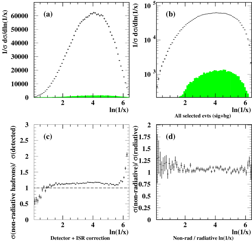
Figure 16: Distributions of $\ln(1/x)$ for 500 pb^-1 of events passing selection cuts. Background from ${\mathrm{W}}^{+}{\mathrm{W}}^{-}$ events is shown as the shaded areas. Figures (c) and (d) show the the typical acceptance and initial state radiation corrections that might be expected.

The expected distribution of $\ln(1/x)$ is shown in figure 16 (a) (and figure 16 (b) with a logarithmic vertical scale) for all events that pass the selection cuts. The statistical errors on the points correspond to a luminosity of 500 pb^-1. The contribution of the ${\mathrm{W}}^{+}{\mathrm{W}}^{-}$ background events is shown as the shaded region. The background is concentrated in the region around the peak of the $\ln(1/x)$ distribution, varies smoothly, and is small compared to the level of the signal events – the signal to background ratio is almost 100:1. In practice, this background could be corrected for by a multiplicative correction factor, the background could be subtracted directly or a more complex matrix correction procedure could be applied.

Typical corrections for detector acceptance and resolution are shown in figure 16 (c). There is a correction of about 10 % to the overall level of the distribution which is basically flat in the region around the peak of the $\ln(1/x)$ distribution. Uncertainties in the determination of detector corrections are therefore unlikely to have a large effect on the position of the peak, and there is no evidence that a serious bias has been introduced into the $\ln(1/x)$ distribution by the event selection. Figure 16 (d) shows the ratio of the $\ln(1/x)$ distributions for events passing the selection cuts that did not radiate and those that radiated a photon of more than 2 GeV. This illustrates the component of the detector correction that accounts for initial state radiation. The bias introduced by the initial state radiation is most severe for low values of $\ln(1/x)$ but is fairly uniform around the area of the peak. It is not expected that the event selection and detector corrections will seriously bias the measurement of the position of the peak.

7.3 Determination of Peak Position

The peak position may be determined by fitting a Gaussian to the ${\mathrm{W}}^{+}{\mathrm{W}}^{-}$-background subtracted $\ln(1/x)$ distribution. The statistical error on the peak position is about 0.025 if data corresponding to 100 pb^-1 are fitted, and this decreases to 0.011 when the expected 500 pb^-1 data sample is analysed. A Gaussian function is only valid for the region close to the peak and is less successful at describing the shape of the distribution far away from it. This leads to a variation of the fitted peak position as data points far from the peak are included in the fit. Varying the fit range such that a reasonable $\chi^{2}$ is still obtained for the fit results in an uncertainty in the peak position of about 0.02.

A systematic error due to uncertainties in the level of the ${\mathrm{W}}^{+}{\mathrm{W}}^{-}$ backgrounds has been estimated by varying the amount of the background subtracted by $\pm 100~{}\%$. The fitted peak position changes by less then 0.01 in all cases. It is not expected that there is a large uncertainty due to the details of the shape of the ${\mathrm{W}}^{+}{\mathrm{W}}^{-}$ background. The process ${\mathrm{W}}^{\pm}\rightarrow{\mathrm{q}}\overline{{\mathrm{q}}}$ is very closely related to ${\mathrm{Z}}^{0}\rightarrow{\mathrm{q}}\overline{{\mathrm{q}}}$ which has been very well understood thanks the the LEP1 data. In conclusion, it is expected that the position of the peak of the $\ln(1/x)$ distribution may be measured with the data recorded at LEP2 to a sufficient precision in order to be able to test the LLA predictions.

7.4 Detailed Shape of ln(1/x) Distribution

The expected statistical errors on the points of the $\ln(1/x)$ distribution are small compared to the bin-to-bin variations of the distribution – there is no apparent scatter of the data points. This indicates that the data will most likely be of sufficient precision to allow a detailed comparison with the shape predicted by theoretical calculations with parameters fitted to LEP1 data. The comments regarding the influence of acceptance, initial state radiation and ${\mathrm{W}}^{+}{\mathrm{W}}^{-}$ background corrections on the peak position also apply to the shape of the distribution – they are not expected to pose a major problem. If these systematic effects turn out to be troublesome, there is the still the prospect that a reasonable measurement of the ratio of $\ln(1/x)$ distributions at LEP1 and LEP2 energies might be made in which many systematic effects may cancel.

It might be expected that the description of data by LLA predictions is more successful at higher energies as the LPHD assumption is more justified. This is supported in part by Monte Carlo studies that indicate that the differences between hadrons and partons are much reduced at LEP2 energies.

7.5 Two Particle Correlation

The two particle correlation at LEP2 energies has been studied in the same way as the single particle $\ln(1/x)$ distribution. If the correlation distribution is computed along lines in the $\ln(1/x_{1})-\ln(1/x_{2})$ plane as in reference [68] then the statistical error on each point would be of the order of 0.02 for the full 500 pb^-1 data ample. This should be compared to 0.005 achieved in reference [68] with about 21 pb^-1 of LEP1 data. Preliminary studies indicate that corrections for acceptance, resolution and initial state radiation will be small as anticipated for this distribution. As for the LEP1 analysis, it is also expected that other systematic effects such as the ${\mathrm{W}}^{+}{\mathrm{W}}^{-}$ background might also cancel when the normalized correlation distribution is calculated.

With the luminosity currently expected from LEP2 it is expected that any measurement of the two particle correlation would be statistics limited. There is however the hope that if the entire data sample is analysed, the possibility exists to test the energy evolution of the predicted correlation distribution in a meaningful way. In particular it can be tested whether the distribution at higher energies may be fitted by a prediction with the coefficients of the next-to-next-to-leading order terms fitted to LEP1 data. Such a prediction with coefficients fitted to LEP1 data is able to describe Pythia/Jetset events at both 91 and 175 GeV. Finally, the ratio of the two particle correlation at 91 and 175 GeV may be measured and compared to the theoretical prediction with the advantage that uncomputed higher order terms may cancel to some extent in the ratio.

7.6 Summary

In summary, measurements of hadron momentum spectra offer the possibility to make detailed tests of LLA QCD predictions, particularly in terms of their energy evolution. The peak position of the $\ln(1/x)$ distribution may be measured accurately with only a small amount of data allowing a powerful test of the extrapolation from lower energies. It should also be possible to determine the detailed shape of this distribution which will provide a stringent test of the energy evolution of predictions from LEP1 energies. Meaningful measurements of the two particle correlation will probably have to wait for the full 500 pb^-1 of luminosity to be delivered by LEP2.

References

- [1] Aleph Collaboration, D. Decamp et al.,Phys. Lett. B255(1991)623.
- [2] Aleph Collaboration, D. Decamp et al.,Phys. Lett. B284(1992)163.
- [3] Delphi Collaboration, P. Abreu et al., Z. Phys. C54(1992)55.
- [4] Delphi Collaboration, P. Abreu et al., Z. Phys. C59(1993)21.
- [5] L3 Collaboration, B. Adeva et al., Phys. Lett. B284(1992)471.
- [6] Opal Collaboration, P.D. Acton et al., Z. Phys. C55(1992)1.
- [7] Opal Collaboration, P.D. Acton et al., Z. Phys. C59(1993)1.
- [8] Opal Collaboration, R. Akers et al., CERN-PPE/95-069, to be published in Z. Phys. C.
- [9] SLD Collaboration, K. Abe et al., Phys. Rev. D51(1995)962.
- [10] S.Bethke, Nucl. Phys. B39(Proc. Suppl.)(1995)198.
- [11] S. Catani, L. Trentadue, G. Turnock and B.R. Webber, Nucl. Phys. B407(1993)3.
- [12] S. Catani, Yu.L. Dokshitzer, M. Olsson, G. Turnock and B.R. Webber, Phys. Lett. B269(1991)432.
- [13] G. Dissertori and M. Schmelling, CERN-PPE/95-119.
- [14] S. Catani and B.R. Webber, private communication.
- [15] T. Sjöstrand, Comp. Phys. Commun. 82(1994)74.
- [16] Opal Collaboration, G. Alexander et al., CERN-PPE/95-126, to be published in Z. Phys.C.
- [17] R.K. Ellis, D.A. Ross and A.E. Terrano, Nucl. Phys. B178(1981)421.
- [18] Yu.L. Dokshitzer and B.R. Webber, Phys. Lett. B352(1995)451.
- [19] B.R. Webber, private communication.
- [20] “QCD”, Z. Kunszt, P. Nason, G. Marchesini and B.R. Webber, from “Z Physics at LEP 1”, CERN 89-08 p. 434, editors G. Altarelli, R. Kleiss and C. Verzagnassi.
- [21] K. Fabricius, G. Kramer, G. Schierholz and I. Schmitt, Z. Phys. C11(1981)315.
-
[22]
A. Bassetto, M. Ciafaloni and G. Marchesini, Nucl. Phys. B163(1980)477;
-
[23]
Yu.L. Dokshitzer, and D.I. Dyakonov, Phys. Lett. B84(1979)234;
G. Parisi and R. Petronzio, Nucl. Phys. B154(1979)427;
G. Curci and M. Greco, Phys. Lett. B92(1980)175;
J.C. Collins and D.E. Soper, Ann. Rev. Nucl. Part. Sci. 37 (1987) 383. - [24] S. Catani and L. Trentadue, Phys. Lett. B217(1989)539, Nucl. Phys. B327(1989)353, Nucl. Phys. B353(1991)183.
- [25] M. Greco, Phys. Rev. D23(1981)2791.
- [26] K. Tesima and M.F. Wade, Z. Phys. C52(1991)43.
- [27] S. Catani, G. Turnock and B.R. Webber, Phys. Lett. B272(1991)368.
-
[28]
J. Kodaira and L. Trentadue, Phys. Lett. B123(1982)335;
J.C. Collins and D.E. Soper, Nucl. Phys. B284(1987)253;
G. Turnock, Cambridge preprint Cavendish–HEP–91/3. - [29] S. Catani, G. Turnock and B.R. Webber, Phys. Lett. B295(1992)269.
- [30] S. Catani, Yu.L. Dokshitzer, F. Fiorani and B.R. Webber, Nucl. Phys. B377(1992)445.
- [31] S. Catani, Yu.L. Dokshitzer and B.R. Webber, Phys. Lett. B322(1994)263. M.H. Seymour, Nucl. Phys. B421(1994)545.
- [32] M.H. Seymour, Nucl. Phys. B436(1995)163.
- [33] M.H. Seymour, CERN preprint CERN-TH/95-225.
-
[34]
D.G. Richards, W.J. Stirling and S.D. Ellis,
Phys. Lett. B119(1982)193;
Nucl. Phys. B229(1983)317 - [35] K.A. Clay and S.D. Ellis, Phys. Rev. Lett. 74(1995)4392, hep–ph/9502223.
- [36] E.W.N. Glover and M.R. Sutton, Phys. Lett. B342(1995)375.
- [37] S. Catani and M. Seymour, in preparation.
- [38] Report of the QCD event generators group, these proceedings.
- [39] W.T. Giele and E.W.N. Glover, Phys. Rev. D46(1992)1980.
-
[40]
G.A. Schuler, PhD thesis, Univ. of Mainz, 1986, Internal Report DESYT-87-01,
Feb. 1987;
B. Lampe, G. Kramer, G. Schierholz and J. Willrodt, Phys. Lett. B79(1978)249, errata Phys. Lett. B80(1979)433. - [41] Aleph Collaboration, D. Buskulic et al., Phys. Lett. B357(1995)487.
-
[42]
Delphi Collaboration, P. Abreu et al., Phys. Lett. B311(1993)408;
Delphi Collaboration, P. Abreu et al., contribution to the EPS-HEP 95 Conference, Brussels, July 1995 (Ref. EPS0551). - [43] P. Nason and B. R. Webber, Nucl. Phys. B421(1994)473.
- [44] N.B. Skachkov, Comm. of the JINR, Dubna 1995, E2-95-189.
-
[45]
V. N. Gribov and L. N. Lipatov, Sov. J. Nucl. Phys. 15(1972)78;
G. Altarelli, G. Parisi, Nucl. Phys. B126(1977)298;
Yu. L. Dokshitzer, Sov. Phys. JETP 46(1977)641. - [46] Yu.L. Dokshitzer, V.A. Khoze, A.H. Mueller and S.I. Troyan, Basics of Perturbative QCD, Editions Frontieres, Gif-sur-Yvette, 1991, and references therein.
- [47] A.H. Mueller, Phys. Lett. 104B(1981)161.
- [48] A. Bassetto, M. Ciafaloni, G. Marchesini and A.H. Mueller, Nucl. Phys. B207(1982)189.
-
[49]
A.H. Mueller, Nucl. Phys. B213(1983)85, Erratum quoted in
Nucl.Phys. B241(1984)141;
Yu.Dokshitzer and S. Troyan, Leningrad preprint LNPI-922(1984). - [50] Yu.L. Dokshitzer, V.A. Khoze and S.I. Troyan, Z. Phys. C55(1992)107.
- [51] Yu.L. Dokshitzer, V.A. Khoze and S.I. Troyan, in: Proc. of the 6th Int. Conf. on Physics in Collisions, p.417, ed. M. Derrick, World Scientific, Singapore, 1987.
- [52] Ya.I. Azimov et al, Z. Phys. C27(1985)65.
- [53] Yu.L. Dokshitzer, V.S. Fadin and V.A. Khoze, Phys. Lett. B115(1982)242; Z. Phys. C15(1982)325.
-
[54]
Yu.L. Dokshitzer, V.A. Khoze, S.I.Troyan,
J.Phys.G: Nucl.Part.Phys. 17(1991) 1481, 1602;
Yu.L. Dokshitzer, Light and Heavy Quark Jets in Perturbative QCD, in: Physics up to 200 TeV, Proc. of the Int. School of Subnuclear Physics, Erice, 1990, vol.28, Plenum Press, New York, 1991. -
[55]
Ya.I. Azimov, Yu.L. Dokshitzer and V.A. Khoze, Sov. J. Nucl. Phys. 36(1982)878;
P.C.Rowson et.al., Phys. Rev. Lett. 54(1985)2580;
V.A. Petrov and O.P. Yushchenko, Z. Phys. C41(1988)521. - [56] Minireview talks given by A.De Angelis and W.J. Metzger at the EPS95 Int. Conf. on High Energy Physics, Brussels, July-August 1995 and references therein.
- [57] B. A. Schumm et.al., Phys. Rev. Lett. 69(1992)3025.
- [58] V.A. Petrov and A.V. Kisselev, Z. Phys. C66(1995)453.
- [59] Delphi Collaboration, contribution eps0542 to the EPS95 Int. Conf. on High Energy Physics, Brussels, July-August 1995
- [60] T. Sjöstrand et al., ”Z Physics at LEP 1”, vol. 3, CERN 89-08, p. 331.
-
[61]
Tasso Collaboration, W. Braunshweig et al., Z. Phys. C45(1989)193;
Aleph Collaboration, D.Decamp et al., Phys. Lett. B273(1991)181 and ref. therein;
Opal Collaboration, R. Akers et al., Phys. Lett. B320(1994)417 and ref. therein. - [62] See, for example, M.Schmelling, CERN/PPE 94-184, p.30; subm. to Physica Scripta.
- [63] See, for example, P.D.Acton et al., Z. Phys. C53(1992)457.
-
[64]
Opal Collaboration, R.Akers et al., Phys. Lett. B352(1995)176;
Opal Collaboration, R.Akers et al., Z. Phys. C61(1994)269. - [65] L.A. del Pozo, Ph.D. Thesis, University of Cambridge 1993. RALT-002.
- [66] Opal Collaboration, M.Z. Akrawy et al., Phys. Lett. B247(1990)617.
- [67] C.P. Fong and B.R. Webber, Nucl. Phys. B355(1991)54.
- [68] Opal Collaboration, P.D. Acton et al., Phys. Lett. B287(1992)401.
- [69] B.R. Webber, in proceedings of XXVI Int. Conf. on High Energy Physics, Dallas, CERN TH 6710/92, (1992).