HIGGS PHYSICS
Conveners:
M. Carena and P.M. Zerwas
Working Group:
E. Accomando,
P. Bagnaia,
A. Ballestrero,
P. Bambade,
D. Bardin,
F. Berends,
J. van der Bij,
T. Binoth,
G. Burkart,
F. de Campos,
R. Contri,
G. Crosetti,
J. Cuevas Maestro,
A. Dabelstein,
W. de Boer,
C. de StJean,
F. Di Lodovico,
A. Djouadi,
V. Driesen,
M. Dubinin,
E. Duchovni,
O.J.P. Eboli,
R. Ehret,
U. Ellwanger,
J.-P. Ernenwein,
J.-R. Espinosa,
R. Faccini,
M. Felcini,
R. Folman,
H. Genten,
J.–F. Grivaz,
E. Gross,
J. Guy,
H. Haber,
Cs. Hajdu,
S.W. Ham,
R. Hempfling,
A. Hoang,
W. Hollik,
S. Hoorelbeke,
K. Hultqvist,
P. Igo–Kemenes,
P. Janot,
S. de Jong,
U. Jost,
J. Kalinowski,
S. Katsanevas,
R. Keränen,
W. Kilian,
B.R. Kim,
S.F. King,
R. Kleiss,
B. A. Kniehl,
M. Krämer,
A. Leike,
E. Lund,
V. Lund,
P. Lutz,
J. Marco,
C. Mariotti,
J.–P. Martin,
C. Martinez–Rivero,
G. Mikenberg,
M.R. Monge,
G. Montagna,
O. Nicrosini,
S.K. Oh,
P. Ohmann,
G. Passarino,
F. Piccinini,
R. Pittau,
T. Plehn,
M. Quiros,
M. Rausch de Traubenberg,
T. Riemann,
J. Rosiek,
V. Ruhlmann-Kleider,
C.A. Savoy,
P. Sherwood,
S. Shichanin,
R. Silvestre,
A. Sopczak,
M. Spira,
J.W.F. Valle,
D. Vilanova,
C.E.M. Wagner,
P.L. White,
T. Wlodek,
G. Wolf,
S. Yamashita,
and F. Zwirner.
1 Synopsis
1. The understanding of the mechanism responsible for the breakdown of the electroweak symmetry is one of the central problems in particle physics. If the fundamental particles – leptons, quarks and gauge bosons – remain weakly interacting up to high energies, then the sector in which the electroweak symmetry is broken must contain one or more fundamental scalar Higgs bosons with masses of the order of the symmetry breaking scale 174 GeV. Alternatively, the symmetry breaking could be generated dynamically by novel strong forces at the scale 1 TeV. However, no compelling model of this kind has yet been formulated which provides a satisfactory description of the fermion sector and reproduces the high precision electroweak measurements.
2. The simplest mechanism for the breaking of the electroweak symmetry is realized in the Standard Model (SM) [1]. To accommodate all observed phenomena, a complex isodoublet scalar field is introduced which, through self-interactions, spontaneously breaks the electroweak symmetry SU(2)U(1)Y down to the electromagnetic U(1)EM symmetry, by acquiring a non–vanishing vacuum expectation value. After the electroweak symmetry breakdown, the interaction of the gauge bosons and fermions with the isodoublet scalar field generates the masses of these particles [2]. In this process, one scalar field remains in the spectrum, manifesting itself as the physical Higgs particle .
The mass of the SM Higgs boson is constrained in two ways. Since the quartic self-coupling of the Higgs field grows indefinitely with rising energy, an upper limit on the Higgs mass is obtained by demanding that the SM particles remain weakly interacting up to a scale [3]. On the other hand, stringent lower bounds on the Higgs mass can be derived from the requirement of stability of the electroweak vacuum [3, 4]. Hence, if the Standard Model is valid up to scales near the Planck scale, then the SM Higgs mass is restricted to the range between GeV and 180 GeV, for a top-quark mass 176 GeV. Moreover, if the Higgs particle is discovered in the mass range up to the GeV accessible at LEP2, this will imply that new physics beyond the Standard Model should exist at energies below a scale of order 10 TeV. [These bounds become stronger (weaker) for larger (smaller) values of the top quark mass].
The high precision electroweak data give a slight preference to Higgs masses of less than 100 GeV, despite the fact that the electroweak observables depend only logarithmically on the Higgs mass through radiative corrections [5]. They do not, however, exclude values up to GeV at the level [6], thus sweeping the entire Higgs mass range of the Standard Model. By searching directly for the SM Higgs particle, the LEP experiments [7] have set a lower bound, GeV [95% CL], on the Higgs mass.
The dominant production mechanism for the SM Higgs boson within the energy range of LEP2 is the Higgs–strahlung process in which the Higgs boson is emitted from a virtual boson [8]. The cross section monotonically falls from pb at 65 GeV down to very small values for Higgs masses near the kinematical threshold. The cross section for the production of Higgs bosons via fusion [9, 10] is nearly two orders of magnitude smaller at LEP2, except at the edge of the phase space for Higgs–strahlung where both are small. In the mass range between 60 and 120 GeV, the dominant decay mode of the SM Higgs particle is [12]. Branching ratios for Higgs decays to and final states are suppressed by an order of magnitude or more.
The experimental search for the SM Higgs boson at LEP2 will be based primarily on the Higgs–strahlung process. The boson can easily be reconstructed in all charged leptonic and hadronic decay channels while the Higgs decay mostly leads to and, less frequently, to final states. Moreover, neutrino decays of the boson, augmented by fusion events, can be exploited in the experimental analyses. Higgs events can be searched for with an average efficiency of about 25%. Exploiting micro–vertex detection for tagging quarks, the Higgs events can be well discriminated from the main background process of production even for a Higgs mass near the mass. When the results of all four LEP experiments are combined, after accumulating an integrated luminosity pb-1 per experiment, the SM Higgs boson can be discovered in the mass range up to 95 GeV at LEP2 for a total center of mass energy of GeV.
3. If the Standard Model is embedded in a Grand Unified Theory (GUT) at high energies, then the natural scale of electroweak symmetry breaking would be close to the unification scale , due to the quadratic nature of the radiative corrections to the Higgs mass. Supersymmetry [13] provides a solution to this hierarchy problem through the cancellation of these quadratic divergences via the contributions of fermionic and bosonic loops [14]. Moreover, the Minimal Supersymmetric extension of the Standard Model (MSSM) can be derived as an effective theory from supersymmetric Grand Unified Theories [15], involving not only the strong and electroweak interactions but gravity as well. A strong indication for the realization of this physical picture in nature is the excellent agreement between the value of the weak mixing angle predicted by the unification of the gauge couplings, and the measured value [15]-[21]. In particular, if the gauge couplings are unified in the minimal supersymmetric theory at a scale GeV) and if the mass spectrum of the supersymmetric particles is of order , then the electroweak mixing angle is predicted to be in the scheme for , to be compared with the experimental result . Threshold effects at both the low scale of the supersymmetric particle spectrum and at the high unification scale may drive the prediction for even closer to its experimental value.
In the past two decades a detailed picture has been developed of the Minimal Supersymmetric Standard Model. In this extension of the Standard Model the Higgs sector is built up of two doublets, necessary to generate masses for up– and down–type fermions in a supersymmetric theory, and to render the theory anomaly–free [22]. The Higgs particle spectrum consists of a quintet of states: two CP–even scalar , one CP-odd pseudoscalar neutral , and a pair of charged Higgs bosons [23] .
Since the tree–level quartic Higgs self–couplings in this minimal theory are determined in terms of the gauge couplings, the mass of the lightest CP-even Higgs boson is constrained very stringently. At tree-level, the mass has been predicted to be less than the mass [24, 25]. Radiative corrections to grow as the fourth power of the top mass and the logarithm of the stop masses. They shift the upper limit to about GeV [26, 27], depending on the MSSM parameters.
The upper limit on depends on , the ratio of the vacuum expectation values associated with the two neutral scalar Higgs fields. This parameter can be constrained by additional symmetry concepts. If the theory is embedded into a grand unified theory, the and Yukawa couplings can be expected to unify at . The condition of - Yukawa coupling unification determines the value of the top-quark Yukawa coupling at low energies [28], thus explaining qualitatively the large value of the top quark mass [18],[29]-[32]. For the present experimental range [33], GeV, the condition of - unification implies either low values of , , or very large values of [29]-[32]. In the small regime, the top-quark mass is strongly attracted to its infrared fixed point [34], implying a strong correlation between the top-quark mass and . The large regime is more complex because of possible large radiative corrections to the quark mass associated with supersymmetric particle loops [35, 36]. For small and GeV, the upper bound on the mass of the lightest neutral Higgs particle is reduced to 100 GeV. This mass bound is just at the edge of the kinematical range accessible at a center of mass energy of 192 GeV [37] – raising the prospects of discovering this Higgs boson at LEP2.
The structure of the Higgs sector in the MSSM at tree level is determined by one Higgs mass parameter, which we choose to be , and . The mass of the pseudoscalar Higgs boson may vary between the present experimental lower bound of 45 GeV [7] and 1 TeV, the heavy neutral scalar mass is in general larger than 120 GeV, and the mass of the charged Higgs bosons exceeds GeV. Due to the kinematics the primary focus at LEP2 will be on the light scalar particle and on the pseudoscalar particle . In the decoupling limit of large mass [yielding large masses], the Higgs sector becomes SM like and the properties of the lightest neutral Higgs boson coincide with the properties of the Higgs boson in the Standard Model [38].
The processes for producing the Higgs particles and at LEP2 are Higgs–strahlung , and associated pair production [39]. These two processes are complementary. For small values of the Higgs boson is produced primarily through Higgs–strahlung; if kinematically allowed, associated production becomes increasingly important with rising . The typical size of the cross sections is of order 1 pb or slightly below. The dominant decay modes of the Higgs bosons are decays into and pairs, if we consider SM particles in the final state [12]. Only near the maximal mass for a given value of do and decays occur at a level of several percent, in accordance with the decoupling theorem. However, there are areas in the SUSY ] parameter space where Higgs particles can decay into invisible LSP final states or possibly other neutralino and chargino final states [40, 41]. If the LSP channel is open, the and invisible decay branching ratios can be close to 100% for small to moderate values of . However, the Higgs boson can still be found in the Higgs–strahlung process. The pseudoscalar , produced only in association with , would be hard to detect in this case since both particles decay into invisible channels for small .
The experimental search for in the Higgs–strahlung process follows the lines of the Standard Model, while for associated production and final states can be exploited. Signal events of the type can be searched for with an efficiency of about 30%; the background rejection is somewhat more complicated than for Higgs–strahlung, due to two unknown particles in the signal final state. For small to moderate , particles with masses up to GeV can be discovered in the Higgs–strahlung process. For large the experimentally accessible limits are typically reduced by about 10 GeV. The pseudoscalar Higgs boson is accessible for masses up to about GeV. [These limits are based on the LEP2 energy of 192 GeV and an integrated luminosity of pb-1 per experiment, with all four experiments pooled.]
The supersymmetric theory may be distinguished from the Standard Model if one of the following conditions occurs: (i) at least two different Higgs bosons are found; (ii) precision measurements of production cross sections and decay branching ratios of can be performed at a level of a few per cent; and (iii) genuine SUSY decay modes are observed. Near the maximum mass, the decoupling of the heavy Higgs bosons reduces the MSSM to the SM Higgs boson except for the SUSY decay modes.
4. In summary. If a neutral scalar Higgs boson is found at LEP2, new physics beyond the Standard Model should exist at scales of order 10 TeV. In the framework of the Minimal Supersymmetric extension of the Standard Model, there are good prospects of discovering the lightest of the neutral scalar Higgs bosons at LEP2. Even though this discovery cannot be ensured, observation or non–observation will have far reaching consequences on the possible structure of low–energy supersymmetric theories.
In section 2 the theoretical analysis and experimental simulations for the search for the Higgs boson in the Standard Model are presented. In section 3 the Higgs spectrum and the couplings in the MSSM as well as the relevant cross sections and branching ratios are studied. In addition, the results of the experimental simulations are thoroughly discussed. Section 4 investigates opportunities of detecting Higgs particles at LEP2 within non-minimal extensions of the SM and the MSSM. In particular, the next–to–minimal extension of the MSSM with an additional isoscalar Higgs field (NMSSM) is studied.
2 The Standard–Model Higgs Particle
2.1 Mass Bounds
(i) Strong interaction limit and vacuum stability. Within the Standard Model the value of the Higgs mass cannot be predicted. The mass is given as a function of the vacuum expectation value of the Higgs field, = 174 GeV, and the quartic coupling which is a free parameter. However, since the quartic coupling grows with rising energy indefinitely, an upper bound on follows from the requirement that the theory be valid up to the scale or up to a given cut-off scale below [3]. The scale could be identified with the scale at which a Landau pole develops. However, in the following the upper bound on shall be defined by the requirement so that characterizes the energy where the system becomes strongly interacting. [This scale is very close to the scale associated with the Landau pole in practice.] The upper bound on depends mildly on the top-quark mass through the impact of the top-quark Yukawa coupling on the running of the quartic coupling ,
| (1) |
with . The first two terms inside the parentheses are crucial in driving the quartic coupling to its perturbative limit. On the other hand, the requirement of vacuum stability in the SM imposes a lower bound on the Higgs boson mass, which depends crucially on the top-quark mass as well as on the cut-off [3, 4]. Again, the dependence of this lower bound on is due to the effect of the top-quark Yukawa coupling on the quartic coupling of the Higgs potential [third term inside the parentheses of eq.(1)], which drives to negative values at large scales, thus destabilizing the standard electroweak vacuum.

Fig.1 shows the perturbativity and stability bounds on the Higgs boson mass of the SM for different values of the cut-off at which new physics is expected. From the point of view of LEP physics, the upper bound on the SM Higgs boson mass does not pose any relevant restriction. The lower bound on , instead, needs to be carefully considered. To define the conditions for vacuum stability in the SM and to derive the lower bounds on as a function of , it is necessary to study the Higgs potential for large values of the Higgs field and to determine under which conditions it develops an additional minimum deeper than the electroweak minimum. The renormalization group improved effective potential of the SM is given by
| (2) |
where and are the tree–level potential and the one–loop correction, respectively. A rigorous analysis of the structure of the potential has been done in Ref.[4]. Quite generally it follows that the stability bound on is defined, for a given value of , as the lower value of for which 0 for any value of below the scale at which new physics beyond the SM should appear. From eq.(1) it is clear that the stability condition of the effective potential demands new physics at lower scales for larger values of and smaller values of .
From Fig.1 it follows that for = 175 GeV and GeV [i.e. in the LEP2 regime] new physics should appear below the scale a few to 100 TeV. The dependence on the top-quark mass however is noticeable. A lower value, 160 GeV, would relax the previous requirement to TeV, while a heavier value 190 GeV would demand new physics at an energy scale as low as 2 TeV.
The previous bounds on the scale at which new physics should appear can be relaxed if the possibility of a metastable vacuum is taken into account [42]. In fact, if the effective potential of the SM has a non-standard stable minimum deeper than the standard minimum, the decay of the electroweak minimum by thermal fluctuations or quantum tunnelling to the stable minimum must be suppressed. In this case, the lower bounds on follow from requiring that no transition at any finite temperature occurs, so that all space remains in the metastable electroweak vacuum. In practice, if the metastability arguments are taken into account, the lower bounds on become gradually weaker. They seem to disappear if the cut-off of the theory is at the TeV scale; however, the calculations are technically not reliable in this energy regime. Moreover, the metastability bounds depend on several cosmological assumptions which may be relaxed in several ways.

(ii) Estimate of the Higgs mass from electroweak data. Indirect evidence for a light Higgs boson comes from the high–precision measurements at LEP [6] and elsewhere. Indeed, the fact that the SM is renormalizable only after including the top and Higgs particles in the loop corrections shows that the electroweak observables should be sensitive to these particle masses. Although the sensitivity to the Higgs mass is only logarithmic, while the sensitivity to the top-quark mass is quadratic, the increasing precision of present experiments makes it possible to derive curves as a function of . Several groups [6] have performed an analysis of by means of a global fit to the electroweak data, including low and high energy data. In the light of the recent direct determination of , the results favor a light Higgs boson. With all LEP, SLD, and N data included, a central value for around 80 GeV and 170 GeV is obtained [6]. However, the recently reported LEP values of and which are more than 2 standard deviations away from the SM predictions, and the left-right asymmetries of SLD which still lead to a 2 discrepancy in compared with LEP analyses, have drastic effects on the SM fits. Fig.2 shows as a function of ; the curve is rather flat at the minimum due to the mild logarithmic dependence of the observables on . It should be noticed in this context that the bounds on become very weak if , and/or the left-right asymmetries are excluded from the data.
In summary. It is clear that the indirect bounds on cannot assure the existence of a light Higgs boson at the reach of LEP2. However, the fact that the best fit to the present high-precision data tends to prefer a light SM Higgs boson, indicates that this particle may be found either at LEP or LHC. On the other hand, the stability bounds imply that if the Higgs boson is light, new physics beyond the Standard Model should appear at relatively low energies in the TeV regime.
2.2 Production and Decay Processes
The main mechanism for the production of Higgs particles in collisions at LEP2 energies is the radiation off the virtual -boson line [8],
| (3) |
The fusion process [9, 10, 11] in which the Higgs bosons are formed in collisions, the virtual ’s radiated off the electrons and positrons,
| (4) |
has a considerably smaller cross section at LEP energies. It is suppressed by an additional power of the electroweak coupling with respect to the Higgs-strahlung process, becoming competitive only at the edge of phase space in (3), where the boson turns virtual. In this corner, however, both cross sections are small and the experimentally accessible mass parameter space will be extended only slightly by the fusion channel.
2.2.1 Higgs-strahlung
The cross section for the Higgs-strahlung process can be written in the following compact form:
| (5) |
where denotes the center-of-mass energy, and , are the charges of the electron; is the usual two-particle phase space function. The radiative corrections to the cross section are well under control. The genuine electroweak corrections [43] are small at the LEP energy, less than 1.5% (for a recent review see Ref.[44]). By contrast, photon radiation [45] affects the cross section in a significant way. The bulk of the corrections, real and virtual contributions due to photons and pairs, can be accounted for by convoluting the Born cross section in eq.(5) with the radiator function ,
| (6) |
with . The radiator function is known to order , including the exponentiation of the infrared sensitive part,
| (7) |
where and are polynomials in and . accounts for virtual and soft photon effects, for hard photon radiation. The ’s are given in Ref.[45].
The cross-section for Higgs-strahlung is shown in Fig.5 for the three representative energy values , and GeV as a function of the Higgs-mass [46]. The curves include all genuine electroweak and QED corrections introduced above. The boson in the final state is allowed to be off-shell, so that the tails of the curves extend beyond the on-shell limit . [The Higgs boson is so narrow, MeV for GeV, that the particle need not be taken off-shell.] From a value of order to pb at GeV, the cross section falls steadily, reaching a level of less than 0.05 pb at the mass GeV.

Since the Higgs particle decays predominantly to and pairs, the observed final state consists of four fermions. Among the possible final states, the channel , the pair being generated by the decay, has a particularly simple structure. Background events of this type are generated by double vector-boson production and with the virtual decaying to and ; final states generate by far the dominant contribution. Since these processes are suppressed by one and two additional powers of the electroweak coupling compared with the signal [except for ], the background can be controlled fairly easily up to the kinematical limit of the Higgs signal. This is demonstrated in Tables 2/2 and Fig. 6 where signal and background cross sections for the process are compared for three Higgs masses at GeV. The invariant mass is restricted to GeV and the invariant mass is cut at GeV. The following conclusions can be drawn from the tables and the figure: (i) The signal-to-background ratio decreases steadily with rising Higgs mass from a value of about three near GeV; (ii) The initial state QED radiative corrections are large, varying between 10 and 20%; (iii) The cross sections are lowered by taking non-zero quark masses into account, but only marginally at a level of less than 1%. Since massless fermions are coupled to spin-vectors in decays but to spin-scalars in Higgs decays, signal and background amplitudes do not interfere as long as quark masses are neglected.
| [GeV] | 65 | 90 | 115 | |
|---|---|---|---|---|
| CompHEP0 | 37.264(58) | 24.395(46) | 10.696(13) | 10.634(13) |
| CompHEP4.7 | 37.147(58) | 24.279(46) | 10.580(13) | 10.518(13) |
| EXCALIBUR | — | — | — | 10.6398(15) |
| FERMISV | — | — | — | 9.49(23) |
| GENTLE0 | 37.3975(37) | 24.4727(25) | 10.7022(11) | 10.6401(11) |
| HIGGSPV | 37.393(27) | 24.490(21) | 10.694(16) | 10.65(05) |
| HZHA/PYTHIA | 36.79(13) | 23.53(13) | 10.28(13) | 10.22(13) |
| WPHACT4.7 | — | — | — | 10.52430.24E-02 |
| WPHACT0 | 37.398960.64E-02 | 24.472690.40E-02 | 10.702720.24E-02 | 10.640700.24E-02 |
| WTO | 37.409940.32E-02 | 24.476530.42E-02 | 10.703600.21E-02 | 10.641570.21E-02 |
| [GeV] | 65 | 90 | 115 | |
|---|---|---|---|---|
| EXCALIBUR | — | — | — | 8.4306(29) |
| FERMISV | — | — | — | 7.90(27) |
| GENTLE0 | 33.7575(34) | 19.4717(19) | 8.47729(85) | 8.43290(84) |
| HIGGSPV | 33.759(12) | 19.480(09) | 8.483(05) | 8.44(05) |
| HZHA/PYTHIA | 33.48(11) | 18.91(11) | 8.31(11) | 8.27(11) |
| WPHACT | 33.752170.16E-01 | 19.469230.91E-02 | 8.476650.57E-02 | 8.432360.57E-02 |
| WTO | 33.777410.10E-01 | 19.485620.83E-02 | 8.485110.78E-02 | 8.440900.78E-02 |
The angular distribution of the bosons in the Higgs-strahlung process is sensitive to the spin-parity quantum numbers of the Higgs particle. At high energies the boson is produced in a state of longitudinal polarization according to the equivalence theorem so that the angular distribution approaches asymptotically the law, where is the polar angle between the flight direction and the beam axis. At non-asymptotic energies the distribution is shoaled [47],
| (8) |
becoming independent of at the threshold. Were a pseudoscalar particle produced in association with the , the angular distribution would be given by , independent of the energy; the polarization would be transverse in this case. Thus, the angular distribution is sensitive to the assignment of spin-parity quantum numbers to the Higgs particle. The coefficients of the term and the constant term are independent and could be modified separately by additional effective , couplings or contact terms induced by interactions outside the Standard Model [48].
2.2.2 The Fusion Process
The final state in which the Higgs particle is produced in association with neutrinos
| (9) |
is built up by two different mechanisms, Higgs-strahlung with decays to the three types of neutrinos and fusion [9, 10, 11, 49, 50]. For final states the two amplitudes interfere. At energies above the threshold for on-shell , Higgs-strahlung is by far the dominant process, while below the threshold the fusion process becomes dominant. Correspondingly, the interference term is most important near the threshold where the cross-over between the two mechanisms occurs. The cross section for Higgs-strahlung above the threshold is of order while below the threshold it is suppressed by the additional electroweak vertex as well as by the off-shell propagator. The fusion cross-section is of order and therefore small at LEP energies where no enhancement factors are effective.111The cross-section for fusion is reduced by another order of magnitude since the leptonic NC couplings are considerably smaller than the CC couplings. The cross section for fusion can be expressed in a compact form [49]:
| (10) |
with and . The more involved analytic form of the interference term between fusion and Higgs-strahlung [11] is given in the Appendix 5.1.
The size of the various contributions to the cross section for the final state is shown in Fig.5 at GeV. The Higgs-strahlung includes all three neutrinos in the final state. The nominal threshold value of the Higgs mass for on-shell production in Higgs-strahlung is GeV at GeV. A few GeV above this mass value the fusion mechanism becomes dominant while the Higgs-strahlung becomes rapidly more important for smaller Higgs masses. In the cross-over range, the cross-sections for fusion, Higgs-strahlung and the interference term are of the same size. With a cross section of the order of 0.01 pb only a few events can be generated in the cross-over region for the integrated luminosity at LEP. Dedicated efforts are therefore needed to explore this domain experimentally and to extract the signal from the event sample , which includes several background channels. Nevertheless, fusion can extend the Higgs mass range that can be explored at LEP2 by a few (perhaps very valuable) GeV.
2.2.3 Higgs Decays
The Higgs decay width is predicted in the Standard Model to be very narrow, being less than 3 MeV for less than 100 GeV. The width of the particle can therefore not be resolved experimentally. The main decay modes (Fig.7), relevant in the LEP2 Higgs mass range, are in the following channels [12, 46]:
| (11) |
The decays are by far the leading decay mode, followed by , charm, and gluon decays at a level of less than 10%. Only at the upper end of the mass range do decays of the Higgs particle to pairs start playing an increasingly important role.
The theoretical analysis of the Higgs decay branching ratios is not only important for the prediction of signatures to define the experimental search techniques. In addition, once the Higgs boson is discovered, the measurement of the branching ratios will be necessary to determine its couplings to other particles. This will allow us to explore the physical nature of the Higgs particle and to encircle the Higgs mechanism as the mechanism for generating the masses of the fundamental particles. In fact, the strength of the Yukawa coupling of the Higgs boson to fermions, , and the couplings to the electroweak gauge bosons, , both grow with the masses of the particles. While the latter can be measured through the production of Higgs particles in the Higgs-strahlung and fusion processes, fermionic couplings can be measured at LEP only through decay branching ratios.
Higgs decay to fermions. The partial width of the Higgs decay to pairs is given by [51]
| (12) |
For the decay into and quark pairs, QCD radiative corrections [52] must be included which are known up to order [in the term up to order ],
| (13) |
accounts for the top-quark triangle coupled to the final state in second order by 2-gluon -channel exchange [53], , while accounts for Higgs decays to two gluons with one gluon split into a pair [12], discussed in detail below. The strong coupling is to be evaluated at the scale , and is the number of active flavors [all quantities defined in the scheme]. The bulk of the QCD corrections can be absorbed into the running quark masses evaluated at the scale ,
| (14) |
In the case of bottom (charm) quarks, the coefficients and are 1.17 (1.01) and 1.50 (1.39), respectively. Since the relation between the pole mass of the charm quark and the mass evaluated at the pole mass is badly convergent, the running quark masses lend themselves as the basic mass parameters in practice. They have been extracted directly from QCD sum rules evaluated in a consistent expansion [54]. Typical values of the running , masses at the scale GeV, which is of the order of the Higgs mass, are displayed in Table 3. The evolution has been performed for the QCD coupling . The large uncertainty in the running charm mass is a consequence of the small scale at which the evolution starts and where the errors of the QCD coupling are very large. In any case the value of the mass, relevant for the prediction of the branching ratio of the Higgs particle, is reduced to about 600 MeV.
| GeV) | ||||
|---|---|---|---|---|
| GeV | GeV | GeV | ||
| GeV | GeV | GeV | ||
| GeV | GeV | GeV | ||
| GeV | GeV | GeV | ||
| GeV | GeV | GeV | ||
| GeV | GeV | GeV |
An additional mechanism for , quark decays of the Higgs particle [12] is provided by the gluon decay mechanism where virtual gluons split into pairs, . These contributions add to the QCD corrected partial widths (13) in which the , quarks are coupled to the Higgs boson directly. As long as quark masses are neglected in the final states, the two amplitudes do not interfere. In this approximation, the contributions of the splitting channels are obtained by taking the differences of the widths between and 4 for , and and 3 for final states, given below in eq.(15). The and the quarks are in general emitted into two different parts of the phase space for the two mechanisms; for the direct process the flight directions tend to be opposite, while by contrast for gluon splitting they are parallel.
The electroweak radiative corrections to fermionic Higgs decays are well under control [55, 44]. If the Born formulae are parametrized in terms of the Fermi coupling , the corrections are free of large logarithms associated with light fermion loops. For , , decays the electroweak corrections are of the order of one percent.
Higgs decays to gluons and light quarks. In the Standard Model, gluonic Higgs decays are primarily mediated by top-quark loops [56]. Since in the LEP2 range Higgs masses are much below the top threshold, the gluonic width can be cast into the approximate form [57]
| (15) |
The QCD corrections, which include the splitting of virtual gluons into and final states, are very important; they nearly double the partial width.
It is physically meaningful to separate the gluon and light-quark decays of the Higgs boson [12] from the , decays which add to the , decays through direct coupling to the Higgs boson. In this case, the partial width is obtained from (15) by choosing for the light , , quarks and by evaluating the running QCD coupling at for three flavors only [corresponding to MeV for ].
Higgs decay to virtual W bosons. The channel becomes relevant for Higgs masses when one of the W bosons can be produced on-shell. The partial width for this final state is given by
| (16) |
with . Due to the larger mass and the reduced NC couplings compared with mass and the CC couplings, respectively, decays to final states are suppressed by one order of magnitude.
Summary of the branching ratios. The numerical results for the branching ratios are displayed in Fig.8, taking into account all QCD and electroweak corrections available so far. Separately shown are the branching ratios for ’s, , quarks, gluons plus light quarks, and electroweak gauge bosons. The analyses have been performed for the following set of parameters: , pole mass , and the masses and as listed in Table 3. The dominant error in the predictions is due to the uncertainty in which migrates to the running quark masses at the high energy scales.
Despite the uncertainties, the hierarchy of the Higgs decay modes is clearly preserved. The branching ratio is more than an order of magnitude smaller than the branching ratio, following from the ratio of the two masses squared and the color factor. Since the charm quark mass is small at the scale of the Higgs mass, the ratio of to is reduced to about , i.e. more than would have been expected naïvely.
Thus, the measurements of the production cross sections and of the decay branching ratios enable us to explore experimentally the physical nature of the Higgs boson and the origin of mass through the Higgs mechanism.
2.3 The Experimental Search for the SM Higgs Particle
Selection algorithms were developed by the four LEP experiments [58] towards the Higgs production via the Higgs-strahlung process, for the following event topologies:
-
(i)
the four-jet channel, ;
-
(ii)
the missing energy channel, ;
-
(iii)
the leptonic channel, anything;
-
(iv)
the channel, hadrons and vice-versa;
altogether amounting to more than 90% of the possible final states in the LEP2 mass range.
All important background processes were included in the simulations. Whenever possible, the corresponding cross-sections were computed and events were generated using PYTHIA 5.7 [59]. The Z process being not simulated in PYTHIA, the corresponding results were derived from a Monte Carlo generator based on Ref.[60]. The most relevant cross-sections are indicated in Table 4 for the three different center-of-mass energies at which the studies were carried out. Events from the Higgs-strahlung process were generated using either PYTHIA (DELPHI, L3, OPAL), the HZGEN generator [61] (DELPHI, for the final state) or the HZHA generator [62] (ALEPH, for all signal final states), and the signal cross-section and Higgs boson decay branching ratios were determined from Ref.[46], or directly from the HZHA program in the case of ALEPH.
| 175 GeV | 192 GeV | 205 GeV | |
|---|---|---|---|
| 173.4 | 135.5 | 116.5 | |
| WW | 14.63 | 17.74 | 18.07 |
| ZZ | 0.45 | 1.20 | 1.43 |
| Z | 2.75 | 2.93 | 3.05 |
| We | 0.68 | 0.90 | 1.10 |
| Z | 0.011 | 0.015 | 0.020 |
| 22.3 | 24.9 | 26.3 |
The selection efficiencies and the background rejection capabilities were evaluated after a simulation of each of the four LEP detectors. Fully simulated events were produced by DELPHI [63, 64], L3 [65] and OPAL [66] for all the background processes and for the signal at several Higgs boson masses, including all the detector upgrades foreseen for the LEP2 running. A fast, but reasonably detailed simulation was used in ALEPH [67] instead, with the current detector design (in particular, the gain expected from the installation of a new vertex detector was conservatively ignored), but it was checked in the four-jet topology and in the missing energy channel, at GeV and with GeV, that this fast simulation faithfully reproduces the predictions of the full simulation chain both for the background rejection and for the signal selection, up to an accuracy at the percent level.
a) Search in the Four-jet Topology
The selection procedures developed by the four collaborations to improve the signal-to-noise ratio are very close to each other. After a preselection aimed at selecting four-jets events, either from global events properties or directly from a jet algorithm such as the DURHAM or JADE algorithms, the four-jet energies and momenta are subjected to a kinematical fit with the four constraints resulting from the energy-momentum conservation, in order to improve the Higgs boson mass resolution beyond the detector resolution. Events consistent with the WW hypothesis, i.e. events in which two pairs of jets have an invariant mass close to , are rejected. Only events in which the mass of one pair of jets is consistent with are kept, and they are fitted again with the Z mass constraint in addition. This last step improves again the Higgs boson mass resolution, which is found to be between 2.5 and 3.5 GeV/ by the four LEP experiments.
However, these requirements do not suffice to reduce the background contamination to an adequate level. This is illustrated in Fig.9a where the distribution of the fitted Higgs boson mass (i.e. the mass of the pair of jets recoiling against the pair consistent with a Z) is shown, for the signal ( GeV/) and for the backgrounds, at GeV and for a luminosity of 500 as obtained from the ALEPH simulation at this level of the analysis.
The high branching of the Higgs boson into must then be taken advantage of to further reduce the background, by requiring that the jets associated to the Higgs boson be identified as b-jets. This is done by means of a microvertex detector, either by counting the charged particle tracks with large impact parameters, or by evaluating the probability that these tracks come from the main interaction point [68], or by directly reconstructing secondary decay vertices [69]. Shown in Fig.9b is the resulting Higgs boson mass distribution after such a b-tagging requirement is applied. The same distribution as seen by DELPHI is shown in Fig.10, together with the efficiency of the DELPHI lifetime b-tagging requirement applied to four-jet events, in which four b-jets, two b-jets or no b-jets are present, as a function of the logarithm of the probability . The OPAL result in this topology is shown in Fig.11a. Due to the recent vertex detector installation, the L3 b-tagging algorithm is not yet fully optimized and its performance is thus expected to improve in the future.
| Experiment | ALEPH | DELPHI | L3 | OPAL |
|---|---|---|---|---|
| Signal | 58 | 43 | 43 | 46 |
| Background | 33 | 33 | 47 | 26 |
The numbers of background and signal events expected to be selected by ALEPH, DELPHI, L3, and OPAL in a window of around the reconstructed Higgs boson mass are shown in Table 5 for a Higgs boson mass of 90 GeV/ and at a center-of mass energy of 192 GeV.
b) Search in the Missing Energy Channel
The four collaborations developed a selection procedure with a sequence of criteria, based on these differences between signal and background, including a b-tagging requirement. The mass of the Higgs boson can be either rescaled or fitted by constraining the missing mass to equal the Z mass, allowing mass resolutions from 3.5 to 5 GeV/ to be achieved. The mass distribution obtained by OPAL in this channel, for a Higgs boson mass of 90 GeV/ and at a center-of mass energy of 192 GeV, is shown in Fig.11b.
This selection procedure was supplemented in DELPHI by an alternative multi-variate probabilistic method, confirming (or slightly improving) the first analysis results. The contribution of the -channel WW fusion to the H final topology was also estimated by DELPHI with the recently released HZGEN event generator which includes both the Higgs-strahlung and the WW fusion diagrams together with their interference. As can be naively expected, the relative gain is only sizeable above the HZ kinematical threshold, and amounts to 28% for a 100 GeV/ Higgs boson at 192 GeV, corresponding to 0.25 additional events expected for an integrated luminosity of 300 .
| Experiment | ALEPH | DELPHI | L3 | OPAL |
|---|---|---|---|---|
| Signal | 24 | 24 | 9 | 25 |
| Background | 13 | 17 | 11 | 20 |
The numbers of background and signal events expected to be selected by ALEPH, DELPHI, L3, and OPAL in a window of around the reconstructed Higgs boson mass are shown in Table 6 for a Higgs boson mass of 90 GeV/ and at a center-of mass energy of 192 GeV.
c) Search in the Leptonic Channel
In addition to these high efficiencies, the mass of the Higgs boson can be determined with a very good resolution (typically better than 2 GeV/) either as the mass recoiling to the lepton pair with the mass of the pair constrained to the Z mass, or with a full fitting procedure using the energies and the directions of the leptons and of the Higgs decay products, the energy-momentum conservation and the Z mass constraint. As shown in Fig.12 from L3, this drastically reduces the ZZ background contamination, except if when the two mass peaks merge together.
The numbers of background and signal events expected to be selected by ALEPH, DELPHI, L3, and OPAL in a window of around the reconstructed Higgs boson mass are shown in Table 7 for a Higgs boson mass of 90 GeV/ and at a centre-of mass energy of 192 GeV.
d) Search in the Channel
| Experiment | ALEPH | DELPHI | L3 | OPAL |
|---|---|---|---|---|
| Signal | 12 | 11 | 7 | 6.5 |
| Background | 12 | 24 | 10 | 9.4 |
The typical efficiency for such an analysis is 20 to 30%, corresponding to 6 to 8 signal events expected for a 90 GeV/ Higgs boson with 1 at 192 GeV, and the and the hadronic mass resolutions amount to approximately 3 GeV/. These resolutions can be further improved by fitting the final state to the HZ hypothesis, with free and constrained. As in the leptonic channel, the only really irreducible background source is the process ZZ when one of the Zs decays into a pair and the other hadronically. The existence of the Higgs boson would then be observed as an accumulation around (, ) in the folded two-dimensional distribution of these masses. A signal-to-noise ratio between 1 and 2 can be achieved when . It could be further improved by a factor of two with a b-tagging requirement, at the expense of a drastic efficiency loss, since two thirds of these events (when ) do not contain b-quarks.
Summary: Numbers of Events Expected
Tables 8, 9 and 10 summarize the
results of the standard model Higgs boson search, with
the total numbers of signal and background events expected by
each experiment given for several Higgs boson masses, at , 192 and 205 GeV, respectively. The uncertainties are due to
the limited Monte Carlo statistics. No systematic uncertainties (due for
instance to the simulation of the b-tagging efficiency) are included.
| (GeV/) | ||||||
|---|---|---|---|---|---|---|
| ALEPH | ||||||
| Signal | ||||||
| Background | ||||||
| DELPHI | ||||||
| Signal | ||||||
| Background | ||||||
| L3 | ||||||
| Signal | ||||||
| Background | ||||||
| OPAL | ||||||
| Signal | ||||||
| Background | ||||||
| ALL | ||||||
| Signal | ||||||
| Background |
| (GeV/) | ||||||
|---|---|---|---|---|---|---|
| ALEPH | Signal | |||||
| Background | ||||||
| DELPHI | Signal | |||||
| Background | ||||||
| L3 | Signal | |||||
| Background | ||||||
| OPAL | Signal | |||||
| Background | ||||||
| ALL | Signal | |||||
| Background |
| (GeV/) | ||||||
|---|---|---|---|---|---|---|
| ALEPH | ||||||
| Signal | ||||||
| Background | ||||||
| DELPHI | ||||||
| Signal | ||||||
| Background | ||||||
| L3 | ||||||
| Signal | ||||||
| Background | ||||||
| OPAL | ||||||
| Signal | ||||||
| Background | ||||||
| ALL | ||||||
| Signal | ||||||
| Background |
2.4 Discovery and Exclusion Limits
Based on the simulations described in Section 2.3, it is possible to derive the exclusion and discovery limits of the standard model Higgs boson as a function of the luminosity for the three center-of-mass energies specified earlier. The contours are defined at for the discovery in the case of the existence of the Higgs boson and at 95% C.L. for the exclusion limits in the case of negative searches, with the specifications described in Appendix 5.3.
In Table 11, the minimum integrated luminosities needed to exclude or discover a given Higgs boson mass at the center-of-mass energies , 192 and 205 GeV are given for the combination of all channels for each of the four experiments separately, as well as for the combination of all channels for the four LEP experiments together. The results of the combination of the four experiments are graphically shown in Fig.13, and summarized in Table 12.
GeV
| Experiment | 65 | 70 | 75 | 80 | |
|---|---|---|---|---|---|
| ALEPH | 12:34 | 18:49 | 25:76 | 36:126 | 80:316 |
| DELPHI | 16:48 | 18:51 | 31:87 | 40:140 | 78:335 |
| L3 | 29:127 | 39:180 | 56:244 | 75:334 | 152:727 |
| OPAL | 17:56 | 20:75 | 34:96 | 44:161 | 74:294 |
| All | 6:15 | 6:19 | 8:28 | 10:41 | 21:90 |
GeV
| Experiment | = 80 | 85 | 90 | 95 |
|---|---|---|---|---|
| ALEPH | 33:117 | 42:166 | 59:238 | 103: 510 |
| DELPHI | 50:195 | 50:231 | 80:388 | 118: 529 |
| L3 | 64:306 | 90:426 | 118:596 | 172: 832 |
| OPAL | 43:157 | 60:251 | 85:360 | 182: 825 |
| All | 12:44 | 15:60 | 20:87 | 33:149 |
GeV
| Experiment | = 80 | 90 | 100 | 105 | 110 |
|---|---|---|---|---|---|
| ALEPH | 41:157 | 80:369 | 76:327 | 119: 504 | 186: 870 |
| DELPHI | 75:356 | 78:372 | 97:462 | 114: 507 | 283:1296 |
| L3 | 74:342 | 142:704 | 162:817 | 164: 897 | 409:2103 |
| OPAL | 87:372 | 149:735 | 151:719 | 267:1284 | 680:3500 |
| All | 16:66 | 25:119 | 30:125 | 38:158 | 72:339 |
| Exclusion: | Discovery: | |||
|---|---|---|---|---|
| (GeV) | (GeV/) | () | (GeV/) | () |
| 175 | 83 | 75 | 82 | 150 |
| 192 | 98 | 150 | 95 | 150 |
| 205 | 112 | 200 | 108 | 300 |
Combining the four LEP experiments, the required minimal integrated luminosity per experiment to discover or exclude a certain Higgs boson mass at a given center-of-mass energy is reduced to approximately a fourth of the average minimal integrated luminosity of each individual experiment. This implies that the maximal value of the Higgs boson mass will be reached at a given energy for luminosities which can be naturally expected at LEP2. The following conclusions can be drawn from detailed analyses of the figures and tables.
-
(i)
At a center-of-mass energy of 175 GeV, the maximum integrated luminosity needed is of the order of 150 and this allows the discovery of a Higgs boson with a maximum mass of about 82 GeV/. Indeed, combining the four experiments it follows that raising the luminosity leads only to a marginal increase of the exclusion and discovery limits, which are very close to each other.
-
(ii)
At 192 GeV it is again sufficient to have an integrated luminosity of about 150 , in this case to discover a Higgs boson with mass up to 95 GeV/. Increasing the center-of-mass energy from 175 to 192 GeV leads to a significant extension in the discovery range of the Higgs boson mass. It is of great interest to observe that at GeV a 95 GeV/ Higgs boson mass can be excluded at the 95% confidence level with an integrated luminosity as low as 33 while with 150 a Higgs boson mass close to 100 GeV/ can be excluded.
-
(iii)
This development continues up to 205 GeV, where a luminosity as low as 70 is sufficient to exclude Higgs boson masses up to about 110 GeV/, and a 5 discovery of a Higgs boson with a mass of order 105 GeV/ requires an integrated luminosity of . More luminosity is needed in this case, since the cross section of the irreducible ZZ background increases. With an integrated luminosity of a Higgs boson mass close to 110 GeV can be discovered.
If each experiment is considered separately, the 5 discovery limit for an integrated luminosity of 500 is, on average, approximately given by 82 (95) (103) GeV/ for = 175 (192) (205) GeV. Similar results may be obtained by combining the four experiments for an integrated luminosity per experiment of about 150 . For the combined exclusion limits, the maximum value of at = 175, 192, 205 GeV is reached for a luminosity per experiment of about 75, 150, 200 . A further increase in luminosity is not very useful in case of negative searches. Clearly, energy rather than luminosity is the crucial parameter to improve the range of masses which can be reached at LEP2.
2.5 The LHC Connection
It has been shown in section 2.4 that LEP2 can cover the SM Higgs mass range up to at a total energy of while the Higgs mass discovery limit increases to for a total energy of . Since this mass range contains the lower limit at which the SM Higgs particle can be searched for at the LHC, the upper limit of the LEP2 energy is quite crucial for the overlap in the discovery regions of the two accelerators.
Low–mass Higgs particles are produced at the LHC predominantly in gluon–gluon collisions [71, 72] or in Higgs–strahlung processes [73, 74],
with the Higgs boson emitted from a virtual boson or from a top quark. In the gluon–fusion process the Higgs particle is searched for as a resonance in the decay channel which comes with a branching ratio of order . Even though large samples of Higgs particles can be generated in this mass range, the signal–to–background ratio is only a few percent and the rejection of jet background events which are eight orders of magnitude more frequent, is a very difficult experimental task. Excellent energy resolution and particle identification is needed [75] to tackle this problem. It has been shown in detailed experimental simulations that the significance of the Higgs signal is expected to rise in this channel from a value at to a value at for if ATLAS and CMS analyses are combined.
In the Higgs–strahlung process, the events can be tagged by leptonic decays of the bosons or the quark to trigger the experiment and to reduce the jet background. In these subsamples the Higgs boson can be searched for in the decay mode with a branching ratio close to unity. This method is based on tagging by micro–vertex detection which is anticipated to be an excellent tool of the LHC detectors. After suitable cuts in the transverse momenta of the isolated lepton and the jets, a peak is looked for in the invariant mass. The experimental significance of this method is biggest for small Higgs masses. For and ATLAS/CMS combined, experimental simulations of the sample suggest that falls from at down to at . It is not yet clear how the search can be extended to higher luminosities where the layers in the micro–vertex detectors closest to the beams may not survive, thus reducing significantly the –tagging performance of the experiments.
Combining the prospective signals from the and the analyses, an overall significance of 7 to 8 may be reached for Higgs masses below , based on a low integrated luminosity of within three years. Raising the integrated luminosity to increases the discovery significance to almost for GeV [76].
3 The Higgs Particles in the Minimal Supersymmetric Standard Model
The Minimal Supersymmetric Standard Model leads to clear and distinct experimental signatures in the Higgs sector. Two Higgs doublets, and , must be present, in order to give masses to the up and down quarks and leptons, and to cancel the gauge anomalies induced through the Higgs superpartners. In the supersymmetric limit, the Higgs potential is fully determined as a function of the gauge couplings and the supersymmetric mass parameter . The breakdown of supersymmetry is associated with the introduction of soft supersymmetry breaking parameters, which are essential to yield a proper electroweak symmetry breaking. In the broken phase, the ratio of the Higgs vacuum expectation values, , appears as a new parameter, which can be related to the other parameters of the theory by minimizing the Higgs potential.
The physical Higgs spectrum of the MSSM contains two CP-even and one CP-odd neutral Higgs bosons, and , respectively, and a charged Higgs boson pair [23]. The tree–level Higgs spectrum is determined by the weak gauge boson masses, the CP–odd Higgs mass, , and . It is only through radiative corrections that the other parameters of the model affect the Higgs mass spectrum. The dominant radiative corrections to the Higgs masses grow as the fourth power of the top-quark mass and they are logarithmically dependent on the sparticle spectrum. The mass of the heavy Higgs doublet is controlled by the CP-odd Higgs mass and, for large values of , the effective low energy theory contains only one Higgs doublet, which couples to fermions in the standard way. In a first approximation, the Higgs masses may be calculated by assuming that all sparticles acquire masses of order of the characteristic supersymmetry breaking scale which, based on naturalness arguments, should be below a few TeV. The low–energy effective theory below is a general two–Higgs doublet model, with couplings which can be calculated as a function of the other parameters of the theory. Under these conditions, a general upper bound on the lightest CP-even Higgs boson mass is derived for values of the CP-odd Higgs mass of order . For smaller values of , a more stringent upper bound is obtained. In the following, we shall discuss in detail the different methods to compute the Higgs spectrum in the MSSM and the bounds which can be derived in each case.
3.1 Higgs Mass Spectrum and Couplings
3.1.1 Tree–level Mass Bounds
The masses of the Higgs bosons at tree level are determined as a function of , and the gauge boson masses as follows,
| (17) |
| (18) |
The mass of the lightest MSSM neutral Higgs particle is bounded to be smaller than the mass [24, 25],
| (19) |
and it approaches this upper bound for large values of . The bound is modified by radiative corrections, which raise the upper limit on the lightest CP-even Higgs mass to values close to 150 GeV.
3.1.2 Radiative Corrections to the Higgs Masses
The one- and partial two-loop radiative corrections to the Higgs mass spectrum in the MSSM have been calculated. Computations implying a variety of different approximations, which may be distinguished according to their level of refinement, exist. In general, the radiative corrections to the Higgs masses are large and positive, being dominated by the contributions of the third-generation quark superfields. Since the upper bound on determines the limit for the detectability of the Higgs boson at LEP2, it is interesting to discuss the different methods in some detail.
a) Diagrammatic Approach. Order by order, a precise method of computation of the radiative corrections to the Higgs masses is the full diagrammatic approach. At the one-loop level such calculations have been pursued by several authors [24, 26, 80]. Complete expressions, including all supersymmetric particle contributions are available [81]. The resulting Higgs masses are defined as the location of the pole in the Higgs propagator. In order to obtain a more accurate estimate of the Higgs spectrum in the diagrammatic approach, the two-loop effects must be evaluated. A first step in this direction was performed in Ref.[82] for the case of large values of the CP-odd Higgs boson mass, large , and degenerate squark masses. It was shown that these corrections may be quite significant, of order 10–15 GeV, underlining the need for a careful treatment of the two-loop effects on the Higgs mass spectrum.
b) Effective Potential Methods. The leading corrections to the Higgs mass spectrum in the MSSM can be computed in a very simple way by means of effective potential methods [27, 78]. If all the contributions from the MSSM particles are included, the results within this scheme differ from those of the full diagrammatic approach in that the Higgs masses are evaluated at zero momentum. In order to simplify the calculations, it is possible to consider only the contributions of the third-generation quark superfields, neglecting all weak gauge coupling effects in the one-loop expressions [27]. This treatment of the effective potential has the virtue of displaying, in a compact way, the full dependence of the one-loop radiative corrections on the stop/sbottom masses and mixing angles. For a given squark spectrum, the numerical results obtained in this case differ by only a few GeV from the results obtained within the full one–loop diagrammatic approach. This reflects the smallness of the one-loop contributions from superfields other than top and bottom. Moreover, it shows that the one-loop vacuum polarization effects relating the Higgs pole masses to the running masses calculated through the effective potential approach are in general small. The effective potential computation can be improved by including the dependence of the stop and sbottom spectrum on the weak gauge couplings [79]. In the limit , , , where are the two stop mass eigenvalues, the expression of the lightest Higgs mass takes a simple form,
| (20) |
where
| (21) |
and
| (22) |
In eq.(22), and the functions and are given by
| (23) |
The above expression is particularly interesting since it provides the upper bound on for a given stop spectrum. Including two–loop effects remains, however, a necessary further step to obtain a correct quantitative estimate of the Higgs mass.
c) Renormalization Group Improvement of the Radiatively Corrected Higgs Sector. The most important two–loop effects may be included by performing a renormalization group improvement of the effective potential, while taking into account, in a proper way, the effect of the decoupling of the heavy third–generation squarks. This program can be easily carried out in the case of a large CP-odd Higgs boson mass and degenerate squarks [77]. Since only one Higgs doublet survives at low energies, the lightest CP–even Higgs mass may be calculated through the renormalization group evolution of the effective quartic coupling, assuming that the heavy sparticles decouple at a common scale . The one-loop renormalization group evolution of the quartic couplings includes two-loop effects through the resummation of the one-loop result. The general result is, however, scale dependent but this dependence is reduced by taking into account the two-loop renormalization group improvement of the one–loop effective potential [84, 85]. The vacuum expectation value of the Higgs field and the renormalized Higgs mass scale (approximately) with the appropriate one–loop anomalous dimension factors within this approximation. The scale dependence of the Higgs mass is cancelled by adding the one-loop vacuum polarization effects, necessary to define the Higgs pole mass. For the case of small stop mixing and large values of , the Higgs spectrum evaluated through this method agrees with the diagrammatic computation at the two–loop level [82, 85].
Analytical Expression for the Lightest CP-even Higgs Mass. The two-loop RG improvement of the one–loop effective potential includes two–loop effects in two different ways: through the resummation of one–loop effects and through genuine two–loop effects. Numerically, the latter are small compared to the resummation effects [83]. Once an appropriate scale of order of the top-quark mass is adopted, the results of the one–loop RG improvement of the tree–level effective potential including the proper threshold effects of squark decoupling, are in excellent agreement with the pole Higgs masses computed by the two-loop RG improvement of the one-loop effective potential [85, 89]. This holds, for large values of the CP-odd Higgs mass, for any value of and the squark mixing angles. Based on this result, an analytical approximation may be obtained [89] which reproduces the dominant two-loop results [85] within an error of less than 2 GeV. Fig.15 shows the agreement of the one–loop and two–loop results for evaluated at the appropriate scale , and the accuracy of the analytical approximation. In the scheme, the pole top-quark mass must be related to the on-shell running mass by taking into account the corresponding one-loop QCD correction factor
| (24) |
Top Yukawa effects have been neglected in eq.(24), since they are essentially cancelled by the two–loop QCD effects. Observe that eq.(24) gives the correct relation between the running and the pole top-quark masses only if the leading-log contributions to the running mass, associated with the decoupling of the heavy sparticles, are properly taken into account and the sparticles are sufficiently heavy so that the finite corrections become small [90]. The analytical approximation to the one-loop renormalization-group improved result, including two-loop leading-log effects, is given by [89]
| (25) | |||||
where the angle is defined at the scale and . is defined above and
| (26) |
Furthermore, with being the one-loop QCD beta function and the number of quark flavours [ at scales below ]. The supersymmetric scale is defined as . For simplicity, all supersymmetric particle masses are assumed to be of order . Notice that eq.(25) includes the leading -term correction [79].


A similar analytical result to eq.(25) has been obtained in Ref.[92]. In this approximation the two-loop leading-logarithmic contributions to are incorporated by replacing in eq.(20) by the running top quark mass evaluated at appropriately chosen scales. For the result is:
| (27) |
where ; the running top-quark mass is given by
| (28) |
with . All couplings on the right hand side of eq.(28) are evaluated at . The requirement that the two stop mass eigenstates be close to each other allows an expansion of the functions and , eq.(23), in powers of . The resulting expression for the Higgs mass is equivalent to the one obtained by performing an expansion of the effective potential in powers of the Higgs field . Keeping only operators up to order four in the effective potential, eq.(27) reproduces the expression of eq.(25). This comparison holds up to small differences associated with the treatment of the effects due to the weak gauge couplings in the one-loop effective potential, and with the inclusion of the top Yukawa effects in the relation between the pole and running top-quark mass [89, 92]. A more detailed treatment of the dependence of the Higgs mass on the weak gauge couplings may be also found in Ref.[91].
Fig.15 shows the comparison between the results of the analytical approximation, eq.(28), and the one-loop RG improvement to the full one–loop leading–log diagrammatic calculation. In general, the prescription given in eq.(28) reproduces the full one-loop RG-improved Higgs masses to within 2 GeV for top-squark masses of 2 TeV or below. The dashed line in the figure shows the result that would be obtained by ignoring the RG-improvement; it reflects the relevance of the two-loop effects in the evaluation of the Higgs mass.
The Case . A similar RG improvement of the effective potential method to the one already discussed can be applied to calculate all the masses and couplings in the more general case of a light CP-odd Higgs boson . As above, the finite one-loop threshold corrections to the quartic couplings at the scale at which the heavy squarks decouple [87] are also taken into account. The effective theory below the scale [86, 87] is a two-Higgs doublet model where the tree–level quartic couplings can be written in terms of dimensionless parameters , , whose tree–level values are functions of the gauge couplings. The one-loop threshold corrections , , are expressed as functions of the supersymmetric Higgs mass and the soft supersymmetry breaking parameters , and [87]. An analytical approximation, which reproduces the previous one–loop RG improved results for all values of and , can also be derived. For example, generalizations of Eq. (20) can be found in Refs.[89, 92]. The CP-even light and heavy Higgs masses and the charged Higgs mass are given as functions of , , , , , the CP-odd Higgs mass and the physical top-quark mass related to the on-shell running mass through eq.(24). The analytical expressions for the masses and mixing angle of the Higgs sector as a function of the parameters are presented in Appendix 5.2. These expressions are the analogue of eq.(25) for the case in which two-Higgs doublets survive at low energies. Effects of the bottom Yukawa coupling, which may become large for values ( being the running bottom mass at the scale ), are also included. A subroutine implementing this method is available [93].
| Vertex | Coupling |
|---|---|
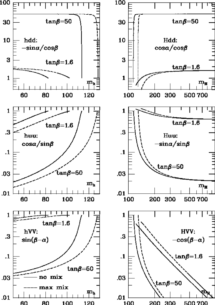
Couplings. Notice that the radiatively corrected quartic couplings , , and hence the corresponding value of the Higgs mixing angle as given in Appendix 5.2, permit us to evaluate all radiatively corrected Higgs couplings. For instance, the Yukawa and gauge Higgs couplings relevant for LEP2 energies are listed in Table 13 [ () is the incoming (outgoing) CP-odd (CP-even) Higgs momentum]. The size of the couplings of the two scalar Higgs bosons to fermions and a gauge boson are shown in Fig.16 [95]. For fermions the charged Higgs particles couple to mixtures of scalar and pseudoscalar currents, with components proportional to and for the two chiralities. The couplings to left(right)-handed ingoing quarks are given by . For large the down–type mass defines the size of the coupling; for small to moderate it is defined by the up–type mass. Furthermore, the trilinear Higgs couplings can be explicitly written as functions of , and [87, 88].
d) Renormalization Group Improvement of the Effective Potential: General Third–Generation Squark Mass Parameters. The above one–loop RG improved treatment of the effective potential relies on the definition of an effective supersymmetric threshold scale, . Its validity is therefore restricted to the case of small differences between the squark mass eigenvalues. Quantitatively, the method is valid if . Furthermore, all the RG Higgs analyses performed in the literature, besides Ref.[91], rely on the expansion of the effective potential up to operators of dimension four. However, to safely neglect higher dimensional operators, the conditions and must be fulfilled.
The case of large splitting in the stop sector is particularly interesting in the light of recent measurements of , whose discrepancy of more than 3 standard deviations with the SM prediction can be ameliorated in the presence of a light higgsino together with a light right–handed stop (see the discussion in the chapter on New Particles) [101]-[104]. The left–handed stop must instead remain reasonably heavy to avoid undesirable contributions to the mass and the leptonic width. It is hence important to generalize the results previously obtained by using the renormalization group improved one-loop effective potential, to the case of general values of the left– and right–handed squark masses and mixing parameters, , , , and , respectively. In this case the contribution of higher dimensional operators to the effective potential must be properly taken into account; hence, the naive treatment in terms of quartic couplings is no longer appropriate.
In Ref.[91], a method has been developed for the neutral Higgs sector of the theory, in which each stop and sbottom particle is decoupled at its corresponding mass scale. Threshold effects, associated with the decoupling of the heavy sparticles, are frozen at the decoupling scales; they evolve, in the squared mass matrix, with the anomalous dimensions of the Higgs fields. The threshold effects achieve a complete matching of the effective potential for scales above and below the decoupling scales, and include all higher order (non–renormalizable) terms arising from the whole MSSM effective potential. The dominant leading–log contributions in the expressions of the renormalized Higgs quartic couplings involve the scale dependent contributions to the effective potential and are treated in the same way as in the RG improved approach described above. The way to proceed in evaluating the CP-even Higgs mass values and mixing angle is explained in detail in Ref.[91]. A subroutine implementing the method is available [94]. This approach makes contact with the computation of the Higgs masses by means of the effective potential performed in Ref.[27]. Moreover, it reproduces the results of Ref.[89] for small mass splitting of the squark masses. This comparison holds up to a tiny difference coming from the inclusion of the small dependence of the one-loop radiative corrections on the weak couplings and the vacuum polarization effects. Indeed, in Ref.[91] the definition of pole Higgs masses is introduced by including the most relevant vacuum polarization effects. The gaugino corrections, which are relatively small, have been also included by incorporating (only) the one-loop leading logarithmic contributions.
3.1.3 Results
The lightest CP–even Higgs mass is a monotonically increasing function of , which in the low regime converges to its maximal value for 300 GeV. In Fig.18 the upper limits on the lightest CP-even Higgs mass [realized in the large limit] are shown as a function of . Since the radiative corrections to the Higgs mass depend on the fourth power of the top mass, the maximal top-quark mass compatible with perturbation theory up to the GUT scale has been adopted for each value of . Apart from the natural choice of the mixing mass–parameters and the scale , this result is the most general upper limit on for a given value of in the MSSM. The variation of the upper bound on as a function of is shown by the solid line (a) of Fig.15. In Fig.18 the mass is plotted for different values of the mixing parameters and . In fact, yields the case of negligible squark mixing, while , characterizes the case of large mixing [i.e. the impact of stop mixing in the radiative corrections is maximized]; yields moderate mixing for large while the mixing effect is close to maximal for low . In Fig.19 we show the masses of the two CP–even Higgs bosons and of the charged Higgs boson as a function of for the case = 1 TeV, 175 GeV and different values of . The peculiar behavior of and for large will be explained in the following.


In general, for very large values of and values of , and of order or smaller than , the mixing in the Higgs sector is negligible and the CP-even Higgs mass eigenstates are approximately given by and . As a result, the properties of h and H mainly depend on the value of . For , one approaches the decoupling limit and the relations and hold. Hence, the CP-even Higgs mass eigenstates are given by and . In this case the lightest CP-even Higgs couples to up (down) fermions as
| (29) |
where is the SM coupling () [Observe that , with ]. The heaviest CP-even Higgs boson, instead, couples in highly non-standard way to fermions,
| (30) |
so that the coupling to up (down) quarks is highly suppressed (enhanced) with respect to the coupling in the Standard Model. For instead, and . Hence, the CP-even Higgs mass eigenstates are given by and . In this case the situation is interchanged; has the non-standard type of couplings to fermions, eq.(30), and has the SM couplings, eq.(29).
The values of the CP-even Higgs masses depend on the size of the or component. When the Higgs is predominantly , its mass is given by eq.(25) for , neglecting the small bottom–quark Yukawa effects. When the Higgs is predominantly , instead, its mass is given by . Hence, the mass of the lightest Higgs boson is given by (and non-standard couplings to fermions) if , and it is given by eq.(25) for larger , for which the couplings to fermions are SM-like. The complementary situation occurs for and this can clearly be observed in Fig.19.
The effects of the bottom quark are only relevant in the limit of large parameters. For values of larger than relevant corrections, which are dependent on the bottom mass, enter the Higgs mass formulae. This can be easily understood in the case , by studying the dependence of on the supersymmetric Yukawa coupling [see appendix 5.2]. For values of of order of , or equivalently for , depends significantly on the fourth power of the parameter. These radiative corrections are negative, lowering the mass of the CP-even Higgs associated with the doublet. Fig.20 shows the case of large .

For large values of and small values of , the charged Higgs mass also receives large negative radiative corrections, which grow as the fourth power of the parameter. Hence, large negative corrections to the charged Higgs mass may be obtained. Such large values of , however, may be in conflict with the stability of the ordinary vacuum state.
3.1.4 Additional Constraints: - Unification and Infrared Fixed Point Structure
The MSSM can be derived as an effective theory in the framework of supersymmetric grand unified theories. In addition to the unification of gauge couplings, the unification of the and Yukawa couplings, , appears naturally in most grand unified scenarios. Given this additional constraint, the experimental values of the and masses at low energies determine the value of as a function of [18, 29, 30]. In fact, for the present experimental range of the top-quark mass GeV [33], the condition of - unification implies either low values of , , or very large values of [18, 29]-[32]. To accommodate - unification, large values of the top Yukawa coupling are necessary in order to compensate for the effects of the renormalization by strong interactions in the running of the bottom Yukawa coupling. Large values of 0.1–1 ensure the attraction towards the infrared (IR) fixed point solution for the top quark mass [34]. The strength of the strong gauge coupling as well as the experimentally allowed range of the bottom mass play a decisive role in this behavior [30]-[32]. In the low case, for the presently allowed values of the electroweak parameters and of the bottom mass and for values of , - unification implies that the top-quark mass must be within ten percent of its infrared fixed point values. A mild relaxation of exact unification [0.85-0.9 1.15] still preserves this feature, especially for values of GeV. In the large region, is and the infrared fixed point attraction, within the context of b- Yukawa coupling unification, is much weaker.
The top-quark mass is also predicted to be close to its infrared-fixed point value in string scenarios, in which the top-quark Yukawa coupling is determined by minimizing the effective potential with respect to moduli fields [99]. Quite generally, the fixed point solution, , is obtained for large values of the top Yukawa coupling at high energy scales, which however remain in the perturbative regime. Within the framework of grand unification, one obtains for GeV, and the running top-quark mass tends to its infrared fixed point value . Hence, relating the running top-quark mass with the pole top-quark mass by taking into account the appropriate QCD corrections we arrive in the low regime at [100],
| (31) |
The strong – correlation associates with each value of at the infrared fixed point the lowest value of consistent with the validity of perturbation theory up to scales of order . If the physical top-quark mass is in the range 160–190 GeV, the values of are restricted to the interval between 1 and 3. This is in agreement with the results from b- Yukawa unification.
The infrared fixed point solution can also be analysed in the large case, where the effects of the bottom Yukawa coupling need to be taken into account in the RG evolution as well. For instance, if the values of the supersymmetric Yukawa couplings of the bottom and top quarks are very close to each other, , the infrared fixed point prediction for the top-quark mass is reduced by a factor with respect to eq.(31) [98, 105]. Still, the values of predicted in this regime are about 190 GeV.
After the above general discussions we shall describe
their consequences for the Higgs sector:
(i) The infrared fixed point structure in the low
region have far-reaching consequences
for the lightest CP-even Higgs mass in the MSSM [96]-[98].
Indeed, for larger than one, the lowest tree–level Higgs mass
is obtained at the lowest value of . Hence, in any theory
consistent with perturbative unification, the fixed point solution
is associated with the lowest value of the tree–level mass consistent
with the theory. Even after including radiative corrections,
the upper bound on the Higgs mass is considerably reduced at the
fixed point solution: for a top mass of 175 GeV, the upper limit
of the Higgs mass
is less than 100 GeV, while for GeV, it is even
less than 80 GeV (see Fig.15).
Hence,
if the infrared fixed point solution for the top-quark with
GeV
is realized in nature, the lightest CP-even Higgs mass must be accessible
at LEP2 for 192 GeV [37, 89].
Fig.15 shows also that for = 175 GeV
the upper bound on the lightest Higgs mass in the case of -
Yukawa coupling unification
is nearly 25 GeV smaller than the
unrestricted MSSM limit.
The present data indicate that the value of is more than above the SM prediction for this quantity. Large positive radiative corrections to are always associated with large values of the Yukawa couplings; they are therefore maximized at the infrared fixed point solution [102, 100]. Moreover, presicion measurements also provide information about the structure of the soft supersymmetry breaking terms: Low values of the right–handed SUSY breaking stop mass and of the SUSY mass parameter are preferred, while the left–handed stop mass parameter must be larger than . For a fixed large value of , the upper bound on the Higgs mass is significantly lower in the case than in the case . Fig21 shows the Higgs mass as a function of for GeV, GeV and consistent with the fixed point solution for GeV, for different values of the mixing mass parameter . Even for the largest value of physically acceptable [i.e. above the experimental lower bound], the Higgs mass remains below 85 GeV. Hence, for the values of the supersymmetry breaking mass terms preferred by the precision electroweak data, associated with a light right-handed stop, lower values of than naïvely expected are obtained.

Furthermore, the most general upper bounds on at the infrared fixed point are valid for very large values of the mixing parameters in the squark sector [, and ] which in general are hard to realize. Requiring radiative breaking of the electroweak symmetry [yet no colour breaking], and imposing the boundary conditions from experimental SUSY mass limits, the range of upper values of is reduced further [100]. In the general framework of supergravity models, various analyses have been performed in the literature to study the spectrum of a constrained MSSM at different levels of refinement [106].
(ii) The condition of - Yukawa coupling unification is also consistent with the values of the top-quark mass measured at the Tevatron for very large values of . There are, however, large uncertainties in this sector associated with one–loop supersymmetric corrections to the bottom mass. These radiative corrections are strongly dependent on the structure of the supersymmetric spectrum and induce strong variations in the predictions for the top-quark mass and , once the unification of the and Yukawa couplings is implemented. Nevertheless, the large regime with unification of the - Yukawa couplings, although more model dependent, provides an interesting framework for Higgs particle searches at LEP2.
Large positive radiative corrections to can also be obtained for large values of , since the supersymmetric bottom–quark Yukawa coupling is enhanced in this regime. Indeed, the value of can be significantly increased if the CP-odd Higgs mass is below 70 GeV [101]-[103]. This is a result of the large positive one-loop corrections associated with the neutral CP-odd Higgs scalar sector of the theory. Low values of the CP-odd Higgs mass, , imply that both the lightest CP-even and the CP-odd Higgs masses would be at the reach of LEP2. The charged Higgs mass is approximately determined through the CP-odd Higgs mass value, , and hence, strong constraints on are obtained from the charged Higgs contributions to . Even conservatively taking into account the QCD uncertainties associated with the branching ratio [i.e. assuming e.g. 40 QCD uncertainties], the decay rate becomes larger than the presently allowed experimental values [107] for GeV, unless the supersymmetric particle contributions suppress the charged Higgs enhancement of the decay rate. The most important supersymmetric contributions to this rare bottom decay come from the chargino-stop one-loop diagram [108]. The chargino contribution to the decay amplitude depends on the soft supersymmetry breaking mass parameter and on the supersymmetric mass parameter . For very large values of , it is given by
| (32) |
where is a function with values of order unity when the characteristic stop mass is of order , and it grows as decreases. For positive (negative) values of the chargino contributions are of the same (opposite) sign as the charged–Higgs contributions. Hence, to partially cancel the light charged–Higgs contributions and render the decay rate acceptable, negative values for are required. This requirement has direct implications on the corrections to the bottom mass mentioned above and puts strong constraints on models with unification of the Yukawa couplings [36, 109].
3.1.5 MSSM Parameters
In the experimental simulations, we have chosen as the two basic parameters of the Higgs sector the mass of the pseudoscalar Higgs boson within the limits 40 GeV 400 GeV, and the angle within the bounds . The upper limit on is introduced merely for convenience, since the variation of with becomes negligible for values of 200–250 GeV. The upper value of is chosen such that the bottom Yukawa coupling remains in the perturbative regime for scales below the grand unification scale. A given value of implies an upper limit on the top mass for which the theory can be extended perturbatively up to the GUT scale. For = 1 this upper limit is already close to 150 GeV so that lower values of would be inconsistent with values of the top quark mass in the experimental range. In the examples we shall discuss, we have chosen:
-
(i)
Top mass, GeV;
-
(ii)
SUSY scale, GeV;
-
(iii)
SUSY Higgs mass parameter and soft SUSY breaking parameter :
and [no mixing];
and [maximal mixing];
[“typical” mixing].
We have taken of order 1 TeV to include the effects of possibly large radiative corrections to the lightest CP-even Higgs mass. In the same way the choice of the soft SUSY breaking parameter and of the SUSY mass parameter is motivated. The central top mass value is close to the central value measured at the Tevatron [33]. The upper and lower bounds are extreme, roughly corresponding to the limits of the CDF measurement. Although the central value for extracted from the LEP precision measurements in the MSSM for large masses of the SUSY particles would be somewhat lower than the central value observed in the Tevatron events, the lower values are still consistent at the level.
3.2 Production and Decay Modes of MSSM Higgs Particles
3.2.1 Higgs Production
The main production mechanisms of the neutral Higgs bosons and in the MSSM at LEP2 energies are through the following processes [110]:
| (33) |
The fusion processes, similar to the Standard Model, play only a marginal role at the kinematical limit of the Higgs-strahlung process for the production of the CP-even Higgs boson . The CP-odd Higgs boson cannot be produced in Higgs-strahlung and in fusion processes to leading order.
The production of the heavy CP-even Higgs particle is very difficult at LEP energies. In the tiny corner of parameter space, for moderate to large , where associated production would be allowed kinematically, the production cross section is suppressed by the small coefficient , due to the coupling discussed earlier, and the threshold P-wave factor. For , , , it is .
The cross sections (33) may be expressed in terms of the cross section for Higgs-strahlung in the Standard Model in the following way [110, 41]:
| (34) | |||||
| (35) |
The factor accounts for the correct suppression of the P-wave cross section near the thresholds. [ is the usual momentum factor of the two particle phase space.] The cross section for fusion of is reduced by the same factor as is the cross section for Higgs–strahlung.
The cross sections for Higgs–strahlung and associated pair production are complementary to each other, coming either with the coefficient or . The cross sections are shown for two representative values of and 50 in Fig.22. The top-quark mass is varied, as usual, between GeV. Since the upper limit on depends strongly on for small values of where the tree-level mass is small, the endpoints of the curves are shifted upwards significantly with increasing top mass. For large values of , on the other hand, the dependence of the upper bound of on the radiative corrections is weaker for rising top mass due to the large value of at the tree level. The supersymmetric coefficient is nearly independent of the top mass and it is very close to unity, so that the spread between the curves is negligible; the coefficient is correspondingly small. In this large case, the curves terminate at the kinematical limit before can be reached, in contrast to the small case. For large the non-zero widths of the particles are taken into account.

For small , Higgs–strahlung provides the largest production cross section while the cross section for associated pair production is much smaller. With at GeV, this mechanism gives rise to a large sample of Higgs particles. For large , associated production is the dominant mechanism with rates similar to the previous case.
The predictions for the cross sections and presented above have been based on the improved effective potential approximation which takes into account heavy (s)quark effects on Higgs masses, mixings and couplings. It turns out a posteriori that this scheme is quite accurate. Indeed, the box contributions to the cross sections are fairly small [111]. This is demonstrated in Fig.23 where the box contributions are compared with the Born term, defined for the effective value . The leading part of the box contributions is generated by the two-Higgs doublet diagrams while the contributions of the genuine SUSY particles are very small.
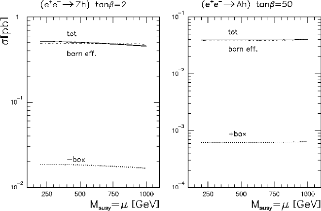
The angular distributions are of the standard form [47] for Higgs–strahlung and spin–zero pair production,
| (38) |
Since the main decay mode of scalar and pseudoscalar Higgs particles
are decays in the MSSM, it is interesting to study the
4–fermion process in greater
detail. The final state includes the signal in the Higgs–strahlung process, and the signal
for associated pair production.
The main component of the background is
production followed by decays. These cross sections
have been evaluated for a cut on the invariant mass of
GeV. The results are shown for a variety of
combinations (, ) in Table 14 for
GeV.
| ( [GeV], ) | (75,30) | (400,30) | (75,1.75) | (400,1.75) | ||
|---|---|---|---|---|---|---|
| no | EXCALIBUR | — | — | — | — | 25.933(10) |
| ISR | HZHA/PYTHIA | 135.17(61) | 23.286(58) | 163.36(75) | 74.04(31) | 22.816(50) |
| with | EXCALIBUR | — | — | — | — | 23.045(23) |
| ISR | HZHA/PYTHIA | 118.60(58) | 18.761(87) | 151.75(75) | 57.74(28) | 18.384(80) |

The cross section for the production of charged Higgs bosons
| (39) |
is built up by -channel and exchanges [41, 112]. It depends only on the charged Higgs mass and no extra parameter,
| (40) |
where the rescaled charges are defined by and and [note that ]; is the velocity of the Higgs particles. The cross section is shown in Fig.24 as a function of the charged Higgs mass for the three representative LEP2 energy values , and GeV. Within the MSSM the present lower limit of the charged Higgs boson mass is about GeV so that only a small window is left for LEP2. Even though the cross section is not particularly small for to 90 GeV, the signal is very hard to extract from the overwhelming background of pair production in this mass range. The analysis of cascade decays [95] can ameliorate the prospects of detecting the charged Higgs boson in this mass range for small .
3.2.2 Decay Modes of the MSSM Higgs Particles
Decays to SM particles. For the lightest CP-even neutral Higgs boson decays almost exclusively to fermion pairs if the mass is less than 100 GeV. Near the upper limit of for a given , i.e. in the decoupling region, the decay pattern becomes SM–like. Fermion pairs are also the dominant decay mode of the pseudoscalar Higgs boson . The partial decay widths of all the neutral Higgs bosons into fermions are given by
| (41) |
in the limit . The couplings have been defined in Table 13. The small additional contributions have been summarized in Ref.[12]. As anticipated from chirality arguments, the widths, including the QCD radiative corrections, do not depend on the parity of the state apart from the overall coupling in the limit of large Higgs masses. For quark decays, has to be chosen as the running quark mass evaluated at the scale . The electroweak corrections are incorporated at a sufficient level of accuracy by adopting the effective potential approximation for the couplings [113].
The partial width for charged Higgs decays to quark pairs is obtained from
| (42) |
This formula is valid if either the first or the second term is dominant. The up and down quark masses are defined again at the mass scale of the charged Higgs boson.
Since the quark couplings to the Higgs bosons are in general strongly enhanced and the quark couplings suppressed in the MSSM [cf. Fig.16], loops may contribute significantly to the coupling so that the approximation cannot be applied any more in general. Nevertheless, it turns out a posteriori that this remains an excellent approximation for the QCD corrections. The CP-even and CP-odd Higgs decays to gluons and light quarks [12] are given by the expressions
| (43) |
where the parentheses refer to the pseudoscalar particle. The form factors are defined by
| (44) |
with for and for . The parameter is defined by the pole mass of the heavy loop quark . In the same way as , the coefficient of the QCD corrections must be evaluated for if gluons and only light quarks are considered in the final state [cf. the SM section for details].
At the edge of the mass range accessible at LEP2, the CP-even Higgs boson can decay into virtual gauge boson pairs . The widths are the same as in the Standard Model, yet suppressed by the MSSM coefficient .
(ii) Cascade decays. A variety of cascade decays could in principle play a role in some ranges of the MSSM parameter space accessible at LEP2, if sufficiently large samples of heavy Higgs bosons were generated. However, for the typical set of parameters discussed in this report, these decay modes are not very important in general and details may be traced back from [95, 114]. The only exception are the cascade decays of the charged Higgs bosons [95] for small to moderate ,
| (45) | |||||
| (46) |
The coefficients depend on the mass ratios of the particles involved,
| (47) | |||||
with and . These decay modes are important for sufficiently light Higgs bosons. If they are allowed, in particular , they reduce the branching ratio considerably, and they overrule decays as the second most important decay channel of the charged Higgs bosons.
Summary of the branching ratios. The branching ratios for the standard quark/lepton/gauge boson and the cascade decay modes discussed above, are shown for “typical mixing” and two representative values and in Fig.25. Unless otherwise specified the top mass in Fig.25 has been fixed to GeV. Increasing the top mass shifts the upper end of the and curves upwards while the and curves are transferred nearly parallel, a consequence of the larger Higgs mass values. The effect of varying is indicated by the hatched bands. The curves labeled and correspond to all mechanisms generating inclusive quarks in the final states, while the curve labeled includes gluons and light quarks. At , interesting cascade decays are predicted for moderately small charged Higgs masses, and ; they affect the experimental search techniques also in the channel by reducing this important decay branching ratio. For large , and decays are overwhelming except in the decoupling regime near the upper limit of the mass.


Predictions for decays of the heavy CP–even Higgs boson are discussed in great detail in Ref.[12].
Neutralino decays. For , Higgs masses up to GeV, there are still windows open for decays into pairs of light neutralinos [41, 115]. These windows have been left by LEP1 and they cannot be closed by LEP1.5 either. The decay channels of interest are
| (48) |
for small to moderate .
Masses and couplings of the states depend on , the gaugino mass parameter , and the Higgs mass parameter . [We assume the relation .] For large and small (positive) values, the lightest neutralino is predominantly built up by the higgsino component while for large values of the light state is predominantly gaugino-like. The couplings of to and are given in terms of the neutralino mixing matrix by
[see e.g. [116]]. Since correspond to the gaugino components of while correspond to the higgsino components, the couplings and can only be non-negligible if the state incorporates both components at a significant level. Moderate values of , are therefore the favorable domain for LSP decays. The widths for the , decays into pairs can be written as
| (49) | |||||
| (50) |
These decays of the Higgs particles are invisible if is stable. The Higgs particle can still be observed in the Higgs-strahlung process through the recoiling at small to moderate where this production channel is dominant. However, the pseudoscalar Higgs boson cannot be detected if, produced in associated production, both particles decay into invisible channels for small to moderate values of .
Since for large the decays of the and Higgs bosons are overwhelming, needs to be small to moderate for decays to be relevant. Typical examples of large branching ratios for Higgs decays to LSP pairs are shown in Fig.26 for a set of gaugino and higgsino mass parameters and . The LSP masses can be read off the threshold values. The branching ratios are large whenever the LSP decay channels are open for . For the LSP decays play a less prominent role; only in a small window close to are the couplings large enough to allow for invisible and decays [115].
3.3 The Experimental Search for the Neutral Higgs Bosons
3.3.1 Searches in the Higgs-strahlung Process
For the hZ process, as well as for HZ when kinematically allowed, all the analyses [58] developed for the standard model Higgs boson and presented in Section 2.3 can be used with no modifications and with a similar efficiency, provided that the Higgs boson decays into supersymmetric particles, such as charginos and neutralinos, are not open. As soon as the decay into a pair of LSPs (Lightest Supersymmetric Particle) is allowed, it may even become dominant therefore rendering the existing analyses ineffective.
Two new selection algorithms were developed by ALEPH to take care of this particular situation where the Higgs boson would decay invisibly, for the following events topologies:
-
(i)
the acoplanar lepton pair topology, ;
-
(ii)
the acoplanar jet topology, .
Only minor modifications to the selection procedure would be needed to extend the validity of these analyses to “almost invisible” Higgs boson decays, such as or when the mass difference between the LSP and the next-to-LSP is small.
a) Search in the Acoplanar Lepton Pair Topology
An efficiency of 45 to 50% was achieved independently of . The lepton momenta were subsequently fitted to the Z mass hypothesis, and the missing mass calculated from the energy-momentum conservation as recoiling against the lepton pair, with a typical resolution of 2 GeV/. Shown in Fig.27 are the mass distributions obtained with 500 at 175 and 192 GeV, for several Higgs boson masses. At 192 GeV, and for , the numbers of signal and background events expected in a window of around the reconstructed Higgs boson mass are 6.2 and 6.1 respectively, assuming a 100% branching fraction into invisible final states.
b) Search in the Acoplanar Jet Topology
Shown in Fig.28 are the mass distributions obtained in the same configurations as in Fig.27, when a tight b-tagging criterion is applied. At 192 GeV, and for , the numbers of signal and background events expected are 7.7 and 4.9 respectively, assuming a 100% branching fraction into invisible final states.
3.3.2 Search in Associated Pair-production Ah
The hA associated production leads to two main final states, in 83% of the cases and in 16% of the cases, if supersymmetric decays are absent.
a) The Topology
This four-jet final state is similar to the four-jet topology arising from
the Higgs-strahlung process, and a similar selection procedure can therefore
be applied. Here, the Z mass constraint cannot be used, and the requirement
of incompatibility with a WW final state must be removed to retain a sizeable
efficiency for the case . However, since the b-quark content
is much higher in this four-b-jet topology than in the Higgs-strahlung process, a
much tighter b-tagging criterion can be applied. In terms of background
rejection, this may even over-compensate the removal of the two previous
requirements while keeping a high efficiency, varying between 10 and 35%.
The four-jet energies and directions can then be fitted to satisfy the total energy-momentum conservation constraint in order to achieve a good mass resolution. Shown in Fig.29a are the distributions of the sum of the fitted and values as obtained in the ALEPH detector with an integrated luminosity of 500 at 175 GeV, for and and 75 GeV/. The same distributions as seen by OPAL are shown in Fig.29b with 500 taken at 192 GeV, for . Since for large values the h and A masses are expected to be close to each other, the mass resolution is expected to improve by imposing this mass equality in the fit procedure. This was done by DELPHI for at 192 GeV, and the result is shown in Fig.30a for an integrated luminosity of 300 . Finally, the distribution of vs that would be obtained in L3 in the mass configuration (60 GeV/, 80 GeV/) if the signal cross-section amounted to 0.5 pb is shown in Fig.30b at 190 GeV, for an integrated luminosity of 1 .
b) The Topology
For this topology, the same analysis as for the Higgs-strahlung process was used
by ALEPH and DELPHI (with the exception that the very last fit intended to improve
the and hadronic mass resolution with the constraint does not apply).
The background level is already very low, except when and are close
to in which case the ZZ background can be reduced by tagging b-quarks.
In this configuration, however, the signal is expected to have a very low
cross-section except at the highest possible center-of-mass energy,
GeV. Altogether, when added to the preceding one, this analysis
increases the selection efficiency of the hA channel by about 20%.
c) The Case h or
If either h or A decays predominantly into , the relevant topology
becomes that of an acoplanar jet pair, as already described in
Section 3.3.1b). However, the pair of jets is actually a pair of
b-quarks in that case, therefore improving the selection efficiency
of a b-tagging criterion with respect to the hZ
configuration.
In the unfortunate situation where both h and A predominantly decay into a pair of LSPs, the resulting final state becomes totally invisible and cannot be found at LEP2. However, in that case, there is a fair chance to discover the lightest supersymmetric particle via a direct neutralino search.
3.4 Discovery and Exclusion Limits
Using the definitions of Appendix 5.3, a minimum signal cross-section was inferred for the hA process from the expected number of background events, both for the discovery and the exclusion. Since the background mass distribution is mostly uniform over the (,) plane, it turns out that this minimum signal cross-section does not depend on and . For instance, at 192 GeV and with an integrated luminosity of 150 , a cross-section in excess of 65 (30) fb can be discovered (excluded) in the hA channel when supersymmetric decays are closed.
For the Higgs-strahlung process, the total cross-section is reduced with respect to the standard model expectation by a factor denoted in the MSSM. The number of events expected is also directly affected by the branching ratio of the h decay into . For each , a minimum value for was inferred for the discovery and the exclusion. The result, which is model-independent, is shown in Fig.32 for the three center-of-mass energies 175, 192 and 205 GeV, with integrated luminosities of 150, 150 and 300 , respectively [58]. The interpretation of the negative searches at LEP1 (from Ref.[117]) is also shown in this plot.
Since this limit becomes irrelevant when supersymmetric decays are dominant, it is supplemented by the 95% C.L. upper limit on invisible final states), as shown in Fig.32.222Since this analysis was done in ALEPH only, it was assumed that the other experiments would contribute in the same proportions as for the visible decays to perform the combination. At LEP2, this limit is worse by about a factor of two than in the case where h predominantly decays into , while it was better at LEP1. In order to make easier the use of these curves to test other models, such as non-minimal supersymmetric extensions of the standard model, the exclusion and discovery limits on are presented in Table 15, for the three center-of-mass energies, and when combining the results at 175 and 192 GeV, on the one hand, and with the 205 GeV results in addition, on the other.
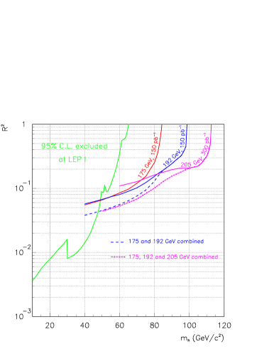
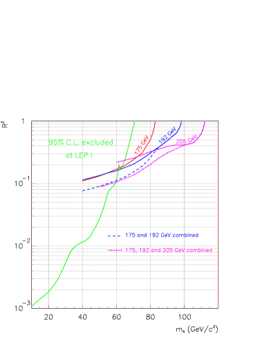
GeV
| (GeV/) | 40 | 50 | 60 | 70 | 75 | 80 | 82 | 83 | 84 |
|---|---|---|---|---|---|---|---|---|---|
| Exclusion | 0.055 | 0.066 | 0.085 | 0.120 | 0.153 | 0.252 | 0.369 | 0.525 | 0.842 |
| Discovery | 0.136 | 0.164 | 0.207 | 0.303 | 0.381 | 0.620 | 0.963 | — | — |
GeV
| (GeV/) | 40 | 50 | 60 | 70 | 80 | 90 | 95 | 97 | 98 |
|---|---|---|---|---|---|---|---|---|---|
| Exclusion | 0.057 | 0.067 | 0.080 | 0.103 | 0.154 | 0.242 | 0.316 | 0.387 | 0.447 |
| Discovery | 0.142 | 0.163 | 0.197 | 0.249 | 0.385 | 0.584 | 0.781 | — | — |
Combination of 175 and 192 GeV
| (GeV/) | 40 | 50 | 60 | 70 | 80 | 90 | 95 | 97 | 98 |
|---|---|---|---|---|---|---|---|---|---|
| Exclusion | 0.038 | 0.045 | 0.056 | 0.076 | 0.129 | 0.242 | 0.316 | 0.387 | 0.447 |
| Discovery | 0.095 | 0.113 | 0.139 | 0.190 | 0.317 | 0.584 | 0.781 | — | — |
GeV
| (GeV/) | 60 | 70 | 80 | 90 | 100 | 105 | 110 | 111 | 112 |
|---|---|---|---|---|---|---|---|---|---|
| Exclusion | 0.109 | 0.127 | 0.162 | 0.196 | 0.207 | 0.222 | 0.315 | 0.375 | 0.481 |
| Discovery | 0.270 | 0.315 | 0.404 | 0.490 | 0.510 | 0.539 | 0.785 | — | — |
Combination of 175, 192 and 205 GeV
| (GeV/) | 50 | 60 | 70 | 80 | 90 | 100 | 105 | 110 | 112 |
|---|---|---|---|---|---|---|---|---|---|
| Exclusion | 0.044 | 0.053 | 0.068 | 0.101 | 0.155 | 0.207 | 0.222 | 0.315 | 0.481 |
| Discovery | 0.111 | 0.132 | 0.168 | 0.252 | 0.370 | 0.510 | 0.539 | 0.785 | — |
To interpret these results in the MSSM framework, both the hA cross-section and the value were computed and compared to the above minimum values in a systematic scan of the (, ) plane, for and for the three different stop mixing configurations, (i) No mixing: and ; (ii) Typical mixing: and (these values of and give a moderate impact of the stop mixing for large but a mixing effect close to maximal if is small); and (iii) Maximal mixing: and , with TeV.
The results of the above analysis are summarized in a series of figures (Figs.33 and 34), which display the areas in the and planes that can be covered for a given energy of LEP2, and 205 GeV at the integrated luminosities 150, 150 and 300 , respectively. The top-quark mass and the stop mixing parameters are varied as specified above. The figures are obtained by combining the four LEP experiments. At = 175 GeV, an increase in luminosity beyond 150 does not improve the potential of the machine for the discovery of the light Higgs boson in any relevant way. The analogous conclusion was reached in the standard model case. At = 192 GeV, still 150 of integrated luminosity per experiment are sufficient to make proper use of the discovery potential of the machine, and a larger luminosity of gives only a slight improvement in the upper bound on the Higgs boson mass which can be discovered or excluded. Although for any center-of-mass energy the variation from 150–200 to 300–400 of integrated luminosity yields a gain of at most 2 to 3 GeV/ in the maximal Higgs boson mass that can be reached, at = 205 GeV the results are presented for 300 since for this energy value the increase in luminosity translates into a quite impressive coverage of .
Comparing the experimental limits for the center-of-mass energies 175 GeV and 192 GeV, Fig.33 a/b and c/d, it is clear that the higher energy value allows a remarkably larger part of the parameter space to be covered. For GeV/ and in particular for GeV, the potential of LEP2 is rather limited at large , while for 192 GeV it is possible to cover the moderate and large for small , (which is a difficult region for LHC). This is especially obvious if non-negligible mixing in the stop sector is considered. For large values of , the limit of the standard model Higgs boson is approached (light gaugino channels are not considered to be open) and the lightest CP-even Higgs boson acquires its maximal value. Since the maximal value of increases with , the range in covered by LEP2 directly reflects the range of standard model Higgs boson masses accessible to the experiments.
|
|
|
|
|
|
|---|
It is interesting to compare the upper limits on which can be reached experimentally, Table 16 and Fig.34, with the maximal h masses expected in the MSSM. In particular, if the experimental limits are compared to the h mass range preferred by gauge and b- Yukawa coupling unification, for 175 GeV/ it can be seen that a large part of the SUSY Higgs mass range is covered in the 192 GeV version of LEP2, in contrast to the lower energy of 175 GeV. In fact, the infrared fixed point solution can be excluded at the 95 C. L. at = 192 GeV if 175 GeV/. (For GeV/ the infrared fixed point solution can be excluded only at 205 GeV.)
3.5 MSSM vs. SM
No precise experimental analyses have yet been developed to cope with the situation in which a Higgs boson would be discovered and thus would need to be studied in detail. This can be partly explained by the relatively low luminosity currently expected at LEP2 which will not allow any accurate measurements to be performed in this field. It could however be imagined that if a new particle were discovered, a substantial extension of the LEP2 project could be decided upon with the purpose of identifying this particle.
The angular distribution of the Higgs boson produced in the Higgs-strahlung process is expected to be quite uniform at the LEP2 center-of-mass energies, and so is the angular distribution of the decay products in the Higgs boson rest frame. Even in the most difficult case , the numbers of events collected by the four experiments with 1 taken at 192 GeV (323 events from the signal and 255 from the backgrounds, see Table 9) suffice to exhibit the flatness of these distributions, and to characterize unambiguously a particle.
Such an excess of events after a b-tagging requirement is also sufficient to claim that this object often decays into , which also characterizes a Higgs particle. However, a precise measurement of the branching fraction can only be done with a channel in which the evidence for a signal can be claimed without b-tagging, i.e. the H topology. This situation is particularly favourable if the Higgs boson mass is not degenerate with the Z mass, in which case the background is much reduced thanks to the excellent recoil mass resolution.
For instance, the cross-section for a 80 GeV/ Higgs boson at GeV in the H topology is 47 fb (after selection cuts, but with no b-tagging requirement), to be compared to 14 fb for the background. This already allows a measurement of the branching fraction (if close to 100%) with a statistical accuracy, if a luminosity of 1 is given to each experiment. Similarly, the quantity can be determined with the same luminosity from the events collected in all the topologies with a statistical accuracy of (resp. 10%) for a 80 GeV/(resp. 90 GeV/) Higgs boson.
Unfortunately, even if the systematics uncertainties were negligible (e.g. the errors related to the b-tagging efficiency determination) this is not sufficient to distinguish the standard model and the MSSM in the region where only the Higgs-strahlung process plays a role. In this region, a statistical accuracy better than 1 or 2% is indeed required [118] to achieve this goal. The extension of the standard model would be manifested in this parameter range only if non-standard Higgs boson decays were observed. It is otherwise only in the region where the hA process or, less likely, charged Higgs bosons (see Section 3.6) can be discovered, that this distinction is possible at LEP2.
3.6 Search for Charged Higgs Bosons
In the MSSM the mass of the charged Higgs bosons is expected to be larger than . In general, for non-extreme stop mixing configuration, it is of the order of , i.e. larger than within a few , rendering rather difficult the discovery of such heavy objects at LEP2. However, this does not hold necessarily in other, e.g. non-minimal supersymmetric extensions of the Standard Model where light charged Higgs bosons – although heavier than 44 GeV/ as shown by LEP1 data – cannot be ruled out. Their discovery would unambiguously signal the existence of an extended Higgs sector.
3.6.1 Production and Decays
Charged Higgs bosons are produced in pairs in the process with a rate depending only on in the general two-doublet model. About 100 such events are expected to be produced with an integrated luminosity of 500 for , irrespective of the center-of-mass energy from 175 to 205 GeV, and this rate decreases rapidly with increasing mass due to the kinematic suppression factor.
Furthermore, if it is assumed that the cascade decay modes [95] like are kinematically suppressed, the charged Higgs bosons are expected to decay predominantly into the heaviest kinematically accessible fermion pair provided it is not suppressed by a small CKM matrix element, i.e. or . Therefore the expected final states are , and , thus leading to an important irreducible background from in addition to the low expected signal rate. This renders almost hopeless the discovery of charged Higgs bosons with mass around and above the W mass.
Searches for these final states have been developed by L3 [119] and DELPHI [64], using full detector simulation of signal and background processes for an integrated luminosity of 500 . A search for the four-jet final state has so far been developed by L3.
a) The Channel
The process leads to four-jet hadronic events.
In order to distinguish a Higgs signal from the main background of
and , use is made of the different
topological properties. The simulated hadronic energy deposits are clustered
into four jets. For example at GeV, for 60 and 70 GeV/ Higgs signals,
75% and 69% selection efficiencies are expected respectively.
The numbers of expected background events are: 3140 , 4664 WW,
and 90 ZZ for 500 .
The four jets can be combined into two jet-pairs in three possible ways, and their energies and directions are fitted to the energy-momentum conservation and to the constraint. The combination with the smallest is chosen, provided that the measured mass difference between the two jet-pairs is smaller than 5 GeV/, and a mass resolution of about 1 GeV/ is achieved. Unlike the channel, no b-tagging requirement can be applied to reject the four-jet background, but the signal-to-noise ratio is improved by removing events where one jet pair combination is consistent with a W pair, at the expense of a suppression of the signal efficiency when .
For , the expected signal efficiency is about 7% and the number of background events is about 2 and 3 WW events, for an integrated luminosity of 500 at GeV.
b) The Channel
The signature of an signal is
one isolated slim jet with missing energy coming from the decay
recoiling against a hadronic system. In the DELPHI analysis, a preselection of hadronic final
states is performed, and the events are clustered into three jets.
The lowest multiplicity jet, i.e. the candidate, is required
to have at most three charged particle tracks.
Further cuts on the mass and on the angle between the two most energetic jets
are applied to reject events without a clear 3-jet topology.
A kinematic fit of the neutrino direction and the momentum (four unknowns)
is performed by constraining the and cs systems to have the same invariant
mass and the total energy-momentum to be conserved (five equations). A cut
is applied to improve the signal-to-noise ratio.
This retains from 16% to 29% of the signal events,
depending on the H± mass and approximately 38 background events
remain for 500 at 175 GeV.
In the L3 analysis, the kinematic fit is replaced by the following approximate method:
-
(i)
the missing momentum, , the missing energy, , and the invariant mass of the two most energetic jets, , are calculated. In order to improve the mass resolution, this mass is rescaled by the factor ;
-
(ii)
for the other hemisphere, the invariant mass is calculated, where is the visible momentum.
The reconstructed masses of and are shown in Fig.35. Cuts as given in the figure are applied. The expected signal efficiencies are about 5.6% and about 2 WW background events are expected for 500 at 175 GeV.
c) The Channel
The events are
characterized by a low particle multiplicity and large missing energy.
The background processes , , WW
and are relevant in this channel.
After applying selection criteria based on the acoplanarity, the total energy and the event thrust axis angle, the main remaining background comes from leptonic WW decays. Unlike the two other channels, a reconstruction of the Higgs boson masses is not possible because of too many unknowns due to the numerous missing energy sources. However, the energies of the decay products of the two taus can be measured, and part of the W decays into e and can be removed by a cut on these two energies, which are expected to be larger in that case than for final states due to the additional neutrinos from the decay.
The expected signal efficiencies are about 12% and about 1 WW background event is expected in the L3 analysis for 500 at 175 GeV. For DELPHI, a 23% signal efficiency is achieved, for a total of 85 background events expected.
3.6.2 Results
In the framework of a general two Higgs doublet model, the results of this analysis can be expressed as a function of Br() (if it is assumed that off-shell decay modes are suppressed) and of . Combining the studies in the , , and channels described in the previous sections, the regions which can be explored with GeV are shown in Fig.36 for luminosities of 100, 200, and 500 taken by one experiment. (These numbers would be roughly divided by four if the four LEP experiments were combined.)
Except for branching ratios into near 0 or 1, all three channels contribute simultaneously which extends the sensitivity range by few GeV/. Charged Higgs bosons with masses up to about 70 GeV/ should be detectable independently of their decay branching ratios assuming a total luminosity of 500 at 175 GeV. The region where a 99.73% CL () effect due to production can be detected is strongly dependent on the assumed luminosity. The boundary lines also depend strongly on the detection sensitivities due to the small change of the charged Higgs boson production cross-section with different . The expected variations of the number of background events for different Higgs masses is taken into account in the figure. The effect of increasing the center-of-mass energy to about 200 GeV is small since only a small change of the production cross section is expected.
The background at LEP2 from WW production with identical decay modes as for the charged Higgs bosons can be controlled. Irreducible background only occurs if . For leptonically decaying Higgs bosons, masses can however be explored up to about due to the small branching fraction of the W boson into .
To summarize, LEP2 has a good potential for a charged Higgs boson discovery already in its first phase at 175 GeV [well beyond the current mass limit of LEP1 of 44 GeV/] as soon as a sufficient luminosity of about 200 is collected. Even with an increase of the machine energy to around 200 GeV, it is extremely difficult to explore the kinematic region around and above because of the large irreducible background from WW production and the low production cross section.
3.7 Complementarity between LEP2 and LHC
As with the SM Higgs boson, it is an important task to compare the Higgs discovery potential of LEP2 with the potential of LHC for the minimal supersymmetric standard model MSSM . The comparison will be based again on the LEP energy with an integrated luminosity of per experiment [yet all four experiments combined] and the presumably ultimate integrated luminosity of LHC, with the results from ATLAS and CMS combined.
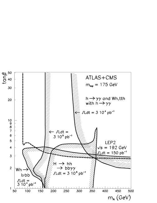

The lightest of the neutral scalar Higgs bosons can be produced at the LHC in gluon–gluon fusion [56, 72], and through Higgs–strahlung off bosons [74] and top quarks [121]. This Higgs particle will be searched for in the and decay channels. Tagging leptonic and decays provides an experimental trigger for the search, but also reduces considerably the huge backgrounds from non– jets. The area of the parameter plane in which the light scalar Higgs boson can be discovered in this way at the LHC is shown in Fig.37 by the shaded regions [122]. The boundary of the LEP2 discovery range is indicated by the full line. No method has yet been found which allows the discovery of in the parameter range of large and between and at either of the two machines.
While the area in which the pseudoscalar Higgs boson can be discovered at LEP is rather modest, a large domain is accessible at LHC, Fig.38. A clean signal of comes from decays; in addition, cascade decays with subsequent leptonic decays provide promising search channels. The search for in decays requires the theoretical control of the top background production at a level between 10 and 2 which is an extremely difficult problem. A similar picture applies to the search for the heavy scalar Higgs particle at the LHC, cf. Fig.38. In particular, the classical four–lepton decay of via intermediate states can be exploited. At LEP2 the heavy Higgs might be produced only in a small region of the MSSM parameter range. The search for charged MSSM Higgs particles is frustrated in either machine. While the LEP2 energy is not sufficient to produce these particles pairwise outside a tiny domain of the MSSM parameter space, the search technique at the LHC is restricted so far to decays with a rather limited range in the charged Higgs mass.
The predictions for the LHC have to be considered with some caution. The computation of the Higgs spectrum and couplings have been treated in analogy to the LEP2 simulations; however, the masses of all SUSY particles have been assumed heavy. Since the couplings in the fusion cross sections as well as in the branching ratios for decays are generated by loops, this channel could be affected strongly by light charginos and stop particles [123]. Depending on the point considered in the SUSY parameter space, the variation of BR through SUSY-loop effects can go either way, enhancing or spoiling the Higgs signal. The problem of SUSY loop corrections is much less severe in search channels which are based on reactions realized already at the Born level, as at the LHC, and all the search channels in collisions. A problem of collisions are the QCD corrections. They are known for the signal in fusion [72], but not for all background processes; the assumption that significances are estimated in a conservative way by setting factors to unity is expected to be fulfilled in large parts of the SUSY parameter space, but this is not guaranteed yet for large . Moreover, if the Higgs bosons do not only decay to SM particles but instead to invisible LSP and other neutralino/chargino states with potentially large branching ratios [41, 115], the analysis must be modified and the conclusions would eventually be altered rather dramatically.
Combining the discovery potentials of LEP2 at and of LHC by summing up all Higgs production channels, the entire parameter plane of the MSSM is predicted to be covered within the standard framework of non–SUSY Higgs decays [based on the parameter set GeV, TeV and ]. The discovery potential of LEP (LHC) in the search for increases for smaller (larger) values of , , and which are associated with smaller (larger) values of . In the region of values less than about 150, the search for can be performed by LEP2 while the other heavy Higgs particles, , and , can be searched for at the LHC. As discussed before, the observation of at least two different Higgs states, at LEP2 or LHC, is a crucial step in disentangling the supersymmetric theory from the Standard Model. Moreover, the channels exploited in the search for are different at LEP2 and LHC. This implies that the couplings involved will be different and hence the physics tested in both cases will be complementary.
4 Non–Minimal Extensions
4.1 The Next–to–Minimal Supersymmetric Standard Model
In this section we shall augment the MSSM by introducing a single gauge singlet superfield leading to a model which is referred to as the NMSSM[124].
The classic motivation for singlets is that they can solve the so-called -problem of the MSSM [125] by eliminating the -term and replacing its effect by the vacuum expectation value (vev) , which may be naturally related to the usual Higgs vev’s . However such models in which the superpotential contains only trilinear terms, possess a symmetry which is spontaneously broken at the electroweak breaking scale. This results in cosmologically stable domain walls [126] which make the energy density of the universe too large. This cosmological catastrophe can be avoided by allowing explicit and non-renormalizable breaking terms suppressed by powers of the Planck mass which will ultimately dominate the wall evolution [127] without affecting the phenomenology of the model. However such terms induce a destabilisation of the gauge hierarchy [128] due to tadpole contributions to the mass in supergravity models with supersymmetry breaking in the hidden sector.
Where does all this leave the NMSSM? This depends on one’s point of view. If there might be some [yet unknown] solution to the domain wall problem, then one can consider models with symmetry which is broken spontaneously. Another approach is to avoid the domain wall problem by considering more general NMSSM models without a symmetry. Note that violating terms, such as a term, large enough to avoid the domain wall problem, can still be sufficiently small as to have no impact on collider phenomenology. These more general models allow arbitrary renormalizable mass terms in the superpotential including the parameter, and linear and quadratic terms in . The question of Planck scale tadpole contributions arises in this case. However, such contributions depend on supersymmetry breaking in a hidden sector of a supergravity theory, and are hence model dependent.
According to this discussion we shall consider two quite different versions of the NMSSM:
(i) The “General NMSSM” is defined by the following superpotential:
| (51) |
This version of the model is essentially a generalization of the MSSM, and provides a more general realization of low-energy SUSY which is equally consistent with gauge coupling unification and high precision measurements. It reduces to the MSSM in the limit in which the field is removed, and since it does not have a symmetry there is no domain wall problem.
(ii) The “Constrained NMSSM” is defined by the trilinear terms in eq.(51), i.e. , plus the constraints of gauge coupling unification and universal soft SUSY-breaking parameters imposed at the unification scale GeV [129, 130].
4.1.1 The General NMSSM
a) Masses and Couplings
The superfield contains a singlet Majorana fermion,
plus a singlet complex scalar. The real part of the
complex scalar will be assumed to develop a vacuum expectation value.
The singlet yields one additional CP-even state and
one additional CP-odd state which are gauge singlets but
can mix with the corresponding neutral Higgs states of the MSSM,
leading to three CP-even Higgs bosons and two
CP-odd Higgs bosons .
Although there are more neutral Higgs bosons than in the MSSM,
they will have diluted couplings due to their singlet components,
making their production cross-sections smaller.
The tree-level CP-odd mass matrix, after rotating away the Goldstone mode as usual, reduces to the matrix in the basis where is the MSSM CP-odd field,
| (52) |
The entries represented by dots are complicated singlet terms. Unlike the MSSM, the parameter here is not a mass eigenvalue due to singlet mixing. The CP-odd matrix is diagonalized by rotating through an angle , leading to two CP-odd eigenstates of mass .
The tree-level CP-even mass squared matrix in the basis is
| (53) |
where, as usual, GeV, ; again the dots correspond to singlet terms. Apart from the terms involving , the upper 22 block of this matrix is identical to the MSSM CP-even matrix. However, whereas the MSSM matrix is diagonalized by rotation through a single angle , the matrix in eq.53 is diagonalized by a 33 unitary matrix , leading to three mass eigenstates with masses ordered as .
The singlets obviously cannot mix with charged scalars, and at tree-level the mass of the charged Higgs is
| (54) |
Clearly a non-zero tends to reduce the charged scalar masses which can now be arbitrarily small, and – in contrast to the MSSM – below the W mass.
We shall define the relative couplings as the coupling in units of the standard model coupling, and similarly we shall define a coupling factor . For example is a generalization of and the are generalizations of in the MSSM. The coupling factorises into a CP-even factor and a CP-odd factor which depends only on the angle which controls singlet mixing in the CP-odd sector.
It can be shown that the CP-even Higgs bosons in this model respect the following relations [131, 132, 133]:
| (55) | |||||
| (56) | |||||
| (57) |
In the case , is equal to the lightest CP-even upper mass bound in the MSSM. The above results show that if we may simply ignore and concentrate on which then becomes the lightest physically coupled CP-even state and must satisfy . Similarly if both and are nearly zero, then .
It can also be shown that
| (58) | |||||
| (59) |
If the lighter CP-odd state is weakly coupled () then it is mainly singlet, and the heavier CP-odd state is then identified with the MSSM state of mass .
b) Theoretical Upper Limit on
According to eq.(57), is clearly a function of
and , and to find the absolute upper bound on the
mass of the lightest CP-even Higgs boson we must maximize this
function (). Radiative corrections, which
drastically affect
the bound [134],
are included using recently proposed methods [89].
For a fixed , the maximum value of is given by the maximum value of as derived from the triviality requirement that none of the Yukawa couplings becomes non-perturbative before the GUT scale of around GeV. Using the recently calculated two-loop RGEs [130], we find an upper limit on as a function of . The maximum value of is typically in the range 0.6-0.7 for a wide range of , depending on and , and falls off to zero for 1.5 or 60 because or , respectively, is very close to triviality. Having derived the maximum value of as a function of , we can use this information to obtain an -dependent maximum value of shown as the upper solid curve in Fig.39. The MSSM bound is also shown (lower solid curve) for comparison. The dashed line is the corresponding upper mass bound in the constrained NMSSM (see later).
As well as being the upper bound on the mass of the lightest CP-even Higgs boson, the parameter plays an important role in constraining all the CP-even Higgs boson masses and couplings. Thus the value of , corresponding to the upper solid line in Fig.39, also constrains and according to eq.(57).

c) Experimental Lower Limits on
has a
theoretical upper limit given by
146 GeV.
Now we shall discuss how experiment may place
a lower limit on which we shall
refer to as . The meaning of
is as follows. For each value of there are many
possible sets of parameters
subject to the bounds in eq.(57).
Each of the three (CP-even) Higgs bosons in each set may
or may not be discovered at LEP, depending on how light
it is and how strongly coupled to the it is.
We can consider the present 95% exclusion
plots at LEP [119] and classify each of the three
Higgs bosons in each set (for a fixed )
as excluded or not excluded. We may find, for some value of ,
that for all
the allowed sets at least one out of the three Higgs bosons
is always excluded. In this case we classify this value of as
being excluded by experiment. We now define as
the largest value of which may be excluded by the LEP
data. There will be a different
for each of the expected LEP2 95% exclusion
plots (see Fig. 32 and Table 15).
If exceeds
then the model is excluded.
is approximately determined by the “worst case” of all three CP-even Higgs bosons having equal masses , and equal couplings . 333This approximate result is exact in the limit that 95% exclusion is equated to 50 produced events. Using this simple approximation, together with current exclusion limits [119], LEP1 already places a limit on of GeV, which is just equal to the mass limit for a CP-even Higgs boson with its coupling suppressed by .
The values of which may be excluded by a future collider of a given energy and integrated luminosity [note that this is total luminosity of all four experiments pooled] are shown in Fig.40 where exclusion is approximately equated to 50 produced events.

Focusing specifically on LEP2, we consider energies and integrated luminosities per experiment of = 175, 192, 205 GeV and = 150, 150, 300 , respectively. Using the exclusion plots [135], we find that LEP2 will yield the exclusion limits GeV respectively, for the three sets of LEP2 machine parameters above. These excluded values of (corresponding to ) are not far from the values of SM Higgs boson masses which may be excluded, due to the steep rise of the exclusion curves in the plane.
d) Exclusion Limits in the Plane
It is possible to obtain
exclusion limits in this model in the plane,
rather similar to the familiar MSSM plots.
The excluded regions are obtained from the following three
searches:
(i) For the processes , we exploit the fact that the upper 22 block of the CP-even mass squared matrix is completely specified (for fixed ) in the - plane. However, unlike the MSSM, the CP-even spectrum is not completely specified since it depends on three remaining unknown real parameters associated with singlet mixing (i.e. the dots in eq.(53)). Nevertheless, since each choice of these parameters completely specifies the parameters and , we can scan over the unknown parameters; if the resulting spectrum is always excluded, then we conclude that this point in the - plane (for fixed ) is excluded. For these excluded regions we use the available LEP1 and LEP2 exclusion lines.
(ii) An excluded lower limit on , as a function of and in this model comes from the non-observation of . The excluded lower limit on in this model is determined by the “worst-case” values of consistent with this value of . It turns out that the worst case experimentally is when the three CP-even Higgs bosons all have equal masses as heavy as possible
| (60) |
and equal coupling factors, , and the two CP-odd Higgs bosons both have masses equal to and , leading to . For these excluded regions we use the simple approximation that 50 events corresponds to exclusion.
(iii) Finally we shall present excluded regions for charged Higgs production, assuming detection up to the kinematic limit. We note that the charged Higgs signal is the same as in the MSSM as considered in Section 3.
In Fig.41 we show the excluded regions of this model corresponding to the choice of parameter 444Strictly speaking if then there is no singlet mixing. However these curves apply to the case where is small (say less than 0.1) and singlet mixing is possible. Such small values of are always found in the constrained NMSSM. for the three sets of LEP2 machine parameters = 175, 192, 205 GeV and = 150, 150, 300 , respectively, and using the LEP1 and LEP2 exclusion data, Fig. 32 and Table 15. In each case the solid lines correspond to exclusion limits from as obtained using procedure (i) above in the NMSSM, the dashed lines correspond to exclusion limits from as obtained using procedure (ii) above in the NMSSM, and the dotted lines correspond to the exclusion limits from charged Higgs production using procedure (iii) above. These exclusion plots should be compared to similar exclusion plots in the MSSM for GeV and degenerate squarks at 1 TeV, which are the parameters assumed in Fig.41.
In Fig.41 we also show a similar plot but with . In this case the solid lines have disappeared beneath the horizon, because for larger the bound may be larger, which allows a heavier CP-even spectrum which is consequently more difficult to exclude. The charged Higgs and channels now give improved coverage, however, since larger decreases the charged Higgs mass, and also decreases the masses for a fixed coupling.
4.1.2 The Constrained NMSSM
As noted in the introduction, the constrained NMSSM is defined by eq.(51) with , , and the condition of universal SUSY-breaking gaugino masses , scalar masses and trilinear couplings at . In addition, the effective potential has to have the correct properties, i.e. the symmetry has to be broken by Higgs vev’s, but the vev’s of charged and/or colored fields as sleptons, squarks and charged Higgs scalars have to vanish. Finally, present lower limits on sparticle masses due to direct searches have to be satisfied, and for the top-quark mass we require values between 150 GeV and 200 GeV.
A priori the constrained NMSSM has six parameters at , three dimensionless couplings , and (the top-quark Yukawa coupling) and three dimensionful ones , and . The scale set by the known mass of the boson reduces the number of free parameters of the model to five. A scan of the parameter space of the model, which is consistent with all the above constraints, has been performed in [129] and [130]. Below we present results, relevant for the Higgs search at LEP2, which are based on the data obtained in [129]. We will discuss the allowed Higgs masses and couplings within the constrained NMSSM.
First note that neither a CP-odd Higgs boson with sufficiently large coupling nor a charged Higgs boson can be sufficiently light within the constrained NMSSM in order to be visible at LEP2. Thus we will concentrate on the neutral CP-even Higgs bosons in the following. Concerning their decays, it follows that neutralinos are too heavy to play a role, thus their branching ratios are close to the standard model ones (essentially ) and the same search criteria apply.
In general, the upper limit on the lightest Higgs mass as a function of the top-quark mass depends on the magnitude of the SUSY-breaking parameters due to radiative corrections to the Higgs potential. For a gluino mass beyond 1 TeV more and more fine tuning is required between these parameters; thus Fig.39 shows the upper limit on the lightest Higgs boson within the constrained NMSSM as a dashed line, for gluinos lighter than 1 TeV.
As noted before, the lightest Higgs boson within the NMSSM can essentially be a gauge singlet state and thus couple very weakly to the boson. Fig.42 (left) shows the logarithm of the coupling as a function of the mass of the lightest Higgs boson. Two different regions exist within the constrained NMSSM: A densely populated region with and GeV, and a tail with (or ) and as small as 10 GeV. Within the tail, the lightest Higgs boson is essentially a gauge singlet state, which explains the small values of .
The solid line in Fig.42 (left) indicates (for GeV) the boundary of the region which can be tested at LEP2 with a maximal c.m. energy of 192 GeV and a luminosity of 150 pb-1; the dotted line corresponds to a maximal c.m. energy of 205 GeV and a luminosity of 300 pb-1 [both after combining all experiments [135]]. A large part of the region with , but only a small part of the tail can be tested.
Fortunately, as noted above, the second lightest Higgs boson cannot be too heavy if the lightest Higgs boson is essentially a gauge singlet state [131], [132], [133]. In the region of the tail of Fig.42 (left), within the constrained NMSSM, the mass of the second Higgs boson varies between 80 GeV and the upper limit indicated in Fig.39 as a dashed line. Its coupling to the boson is very close to 1 if . Fig.42 (right) shows the logarithm of the coupling as a function of the mass of the second lightest Higgs. The tail of Fig.42 (left) corresponds to the region with in Fig.42 (right) and . Thus, a small part of the parameter space corresponding to the tail of Fig.42 (left) actually becomes visible at LEP2 through the observation of , which behaves like the lightest Higgs boson of the MSSM in this case.
If a Higgs boson is observed, it will generally be very difficult, however, to distinguish the NMSSM from the MSSM [130]. This seems only possible if a Higgs boson happens to contain a sizeable amount of the singlet state (and hence a measurably reduced coupling to the boson), but couples still strongly enough in order to be visible. Finally, the constrained NMSSM could actually be ruled out at LEP2 if a neutral CP-odd Higgs particle, a charged Higgs particle, or an invisibly decaying Higgs particle would be observed.
4.2 Non-linear Supersymmetry
Most of the supersymmetric models investigated so far are models based on linearly realized supersymmetry. However, supersymmetry may as well be realized nonlinearly. Whereas the linear supersymmetric models require supersymmetric partners for all conventional particles in the standard model, the nonlinear models do not lead to SUSY partners. Most global nonlinear supersymmetric models require only one new particle: the Akulov-Volkov field [136], which is a Goldstone fermion. This Goldstino can be removed by going over to curved space, i.e. to supergravity, where it can be gauged away. In the flat space limit, the supergravity multiplet decouples from ordinary matter so that supersymmetry can manifest itself only in the Higgs sector.
The formalism for extending the standard model to a supersymmetric theory in a nonlinear way was developed in ref.[137]. Recently, the general form of the nonlinear supersymmetric standard model has been constructed and the Higgs potential in the flat space limit [138] has been derived.
The Higgs sector of the nonlinear SUSY models is evidently larger than that of the Standard Model. It contains at least two dynamical Higgs doublets and an auxiliary Higgs singlet. In the case that both the dynamical and the auxiliary singlet are included in the theory, the spectra of Higgs bosons in the nonlinear models resemble those of the linear model with two Higgs doublets and one singlet (NMSSM). Both models have three scalar, two pseudoscalar Higgs bosons and one charged Higgs boson pair. However, the structure of the Higgs potential is quite different between nonlinear models and the NMSSM. For the general nonlinear model, the complete potential in the flat space limit is given by [138]
| (62) | |||||
involving novel types of interactions between the Higgs fields. The two Higgs doublets and the singlet develop the vev’s respectively. The three scalar Higgs bosons are the eigenstates of the scalar-Higgs mass matrix. In a way similar to the NMSSM, an upper bound for the mass of the lightest scalar Higgs boson can be derived at the lowest order,555In the present exploratory analysis we have neglected the radiative corrections.
| (63) |
where . Hence, for and for . In the latter case, the upper bound of determines the limit of . For GeV and with the GUT scale as cut-off scale, one obtains GeV. Even though at the c.m. energies of 175, 192, and 205 GeV for LEP2 the production of may be kinematically possible, the production rate is in general not large enough for to be detected. The main contributions to the production cross sections come from (i) the Higgs-strahlung process; (ii) the process where is radiated off leptons or quarks, and (iii) associated pair production , where is a pseudoscalar Higgs boson.
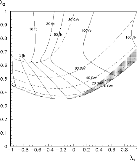
We have first searched for parameter regions where the experimental lower limit on given by the LEP1 data is minimal; it turned out that there are regions where even is still allowed. Fig.43 shows (dashed) the contour lines of and (full) the contour lines of the cross section for the production of in collisions at , in the plane for a representative set of the parameters and ( being the charged-Higgs mass). In the shaded region, the cross section at is greater than 1 pb, which corresponds to the discovery limit of LEP1 for [135]. This region is excluded by LEP1 since the discovery limit decreases with decreasing . The discovery limit at with a luminosity of 500 is about 50 fb for (about 30 fb for ) [135]. Thus the region accessible at LEP2 includes the area in Fig.43 where and 50 fb. As with LEP1, a massless could be undetectable.
For some parameter sets, the nonlinear SUSY model may be tested even if the lightest scalar is undetectable. If the production cross section of is smaller than the discovery limit, one can examine whether the production of the other Higgs bosons is kinematically possible and whether their production rates are large enough for discovery.
For the higher energies 192 and 205 GeV, the effects are similar to the 175 GeV case. Though the accessible region increases, an undetectable massless Higgs boson is still possible. Energies of 240 GeV and more are needed to test this nonlinear supersymmetric model conclusively.
4.3 Majoron Decays of Higgs Particles
There are a variety of well motivated extensions of the Standard Model (SM) with a spontaneously broken global symmetry. This symmetry could either be lepton number or a combination of family lepton numbers [139, 140]. These models are characterized by a more complex symmetry breaking sector which contains additional Higgs bosons. It is specially interesting for our purposes to consider models where such symmetry is broken at the electroweak scale [141, 142]. In general, these models contain a massless Goldstone boson, called majoron (), which interacts very weakly with normal matter. In such models, the normal doublet Higgs boson is expected to have sizeable invisible decay modes to the majoron, due to the strong Higgs–majoron coupling. This can have a significant effect on the Higgs phenomenology at LEP2. In particular, the invisible decay could contribute to the signal of two acoplanar jets and missing momentum. This feature of majoron models allows one to strongly constrain the Higgs mass in spite of the occurrence of extra parameters compared to the SM. In particular, the LEP1 limit on the predominantly doublet Higgs mass is close to the SM limit irrespective of the decay mode of the Higgs boson [143, 144].
We consider a model containing two Higgs doublets () and a singlet () under the group. The singlet Higgs field carries a non-vanishing charge, which could be lepton number. Here we only need to specify the scalar potential of the model:
| (64) | |||||
where the sum over repeated indices =1,2 is assumed.
Minimization of the above potential leads to the spontaneous symmetry breaking and allows us to identify a total of three massive CP even scalars (i=1,2,3), plus a massive pseudoscalar and the massless majoron . We assume that at the LEP2 energies only three Higgs particles can be produced: the lightest CP-even scalar , the CP-odd massive scalar , and the massless majoron . Notwithstanding, our analysis is also valid for the situation where the Higgs boson is absent [145], which can be obtained by setting the couplings of this field to zero.
At LEP2, the main production mechanisms of invisible Higgs bosons are the Higgs-strahlung process () and the associated production of Higgs bosons pairs (), which rely upon the couplings and respectively. The important feature of the above model is that, because of its singlet nature, the majoron is not sizeably coupled to the gauge bosons and cannot be produced directly, thereby evading strong LEP1 constraints. The and couplings depend on the model parameters via the appropriate mixing angles, but they can be effectively expressed in terms of the two parameters , :
| (65) | |||||
| (66) |
The couplings are model dependent. For instance, the SM Higgs sector has and , while a majoron model with one doublet and one singlet leads to and .
The signatures of the Higgs-strahlung process and the associated production depend upon the allowed decay modes of the Higgs bosons and . For Higgs boson masses accessible at LEP2 energies the main decay modes for the CP-even state are and . We treat the branching fraction as a free parameter. In most models is basically unconstrained and can vary from 0 to 1. Moreover we also assume that, as it happens in the simplest models, the branching fraction for is nearly one, and the invisible decay modes , do not exist (although CP-allowed). Therefore our analysis depends upon five parameters: , , , , and . This parameterization is quite general and very useful from the experimental point of view: limits on , , , , and can be later translated into bounds on the parameter space of many specific models.
The parameters defining our general parameterization can be constrained by the LEP1 data. In fact Refs.[143, 146] analyze some signals for invisible decaying Higgs bosons, and conclude that LEP1 excludes up to 60 GeV provided that . Similar results are obtained in fig.(32).
The topology is our main subject of investigation and we carefully evaluate signals and backgrounds, choosing the cuts that enhance the signal over the backgrounds. Our goal is to evaluate the limits on , , , , and that can be obtained at LEP2 from this final state. There are three sources of signal events with the topology 2 -jets: one due to the associated production and two due to the Higgs–strahlung.
| (67) | |||||
| (68) | |||||
| (69) |
The signature of this final state is the presence of two jets containing quarks and missing momentum (). It is interesting to notice that for light and , the associated production dominates over the Higgs–strahlung mechanism [146].
There are several sources of background for this topology:
where the particles in square brackets escape undetected and the jet originating from the quark is identified (misidentified) as being a -jet.
At this point the simplest and most efficient way to improve the signal-over-background ratio is to use that the and decays lead to jets containing -quarks. So we require that the events contain two -tagged jets. Moreover, the background can be further reduced requiring a large . We therefore have imposed a set of cuts which is based on the cuts used by the DELPHI collaboration for the SM Higgs boson search [63].

|

|
Depending on the and mass ranges, including or excluding an invariant mass cut GeV [where is the mass of the particle decaying visibly] gives better or weaker limits on the and couplings. Therefore, for each mass combination four limits are calculated (with or without invariant mass cut, with thrust cut or the cut on the minimal two-jet energy) and the best limit is kept.
We denote the number of signal events for the three production processes (67 – 69), after imposing all cuts, , , and respectively, assuming that . Then the expected number of signal events when we take into account couplings and branching ratios is
| (70) |
In general, this topology is dominated by the associated production, provided it is not suppressed by small couplings or phase space. The most important background after the cuts is production. The total numbers of background events summed over all relevant channels are 2.3, 2.8 and 5.9 for , and GeV respectively.
In order to obtain the limits shown in Figs.45-45, we assumed that only the background events are observed, and we evaluated the 95 % CL region of the parameter space that can be excluded with this result. By taking the weakest bound, as we vary , we obtained the absolute bound on , , and independent of the decay mode. The limits on obtained by searches for the final states are stronger than those obtained from the topology. Moreover, the bounds in the limiting case apply for the simplest model of invisibly decaying Higgs bosons, where just one singlet is added to the SM. A more complete presentation of these results will be given in Ref.[147].
4.4 Strongly Interacting Higgs Particle
The radiative corrections at LEP1 depend only logarithmically on the Higgs mass, and the measurements, although very precise, are not sufficient to determine the structure of the Higgs sector. It is therefore necessary to keep an open mind to the possibility that the Higgs sector is more complicated than in the Standard Model. Beyond the Standard Model various extensions have been suggested. One of the possibilities is supersymmetry which has been previously discussed. Another possibility is strong interactions in the form of technicolor, which at least in its simplest form is ruled out by the LEP1 data. Strong interactions in the Standard Model itself imply a heavy Higgs boson and can presumably be studied at the LHC.
However, the idea of strong interactions is more general. In particular it is possible that strong interactions are present in the singlet sector of the theory. In general the choice of representations in a gauge theory is arbitrary and presumably a clue to a deeper underlying theory. Singlets do not have quantum numbers under the gauge group of the Standard Model. They therefore do not feel the strong or electroweak forces, but they can couple to the Higgs particle. As a consequence, radiative corrections to weak processes are not sensitive to the presence of singlets in the theory, because no Feynman graphs containing singlets appear at the one–loop level. Because effects at the two–loop level are below the experimental precision, the presence of a singlet sector is not ruled out by any of the LEP1 precision data.
It is therefore not unreasonable to assume that there exists a hidden sector that affects Higgs physics only. Such an extension of the Standard Model involving singlet fields preserves the essential simplicity of the model, while at the same time acting as a realistic model for non–standard Higgs properties. Here we will study the coupling of a Higgs boson to an symmetric set of scalars, which is one of the simplest possibilities introducing only a few extra parameters in the theory. The extra scalars may give rise to large invisible decay width of the Higgs particle. When the coupling is large enough, the Higgs resonance can become wide even for a light Higgs boson. This has led to the conclusion that this Higgs particle becomes undetectable at the LHC [148]. As one can measure missing energy more precisely at colliders than at a hadron machine, LEP2 can give important constraints on the parameters of the model. However, it is clear that there will be a range of parameters where this Higgs boson can be seen neither at LEP nor at the LHC.
a) The Model
The Higgs sector of the model is described by the following Lagrangian,
where is the normal Higgs doublet and the vector is an N–component real vector of scalar fields, which we call phions. Couplings to fermions and vector bosons are the same as in the Standard Model. The ordinary Higgs field acquires the vacuum expectation value . We assume that the –field acquires no vacuum expectation value, which can be assured by taking positive. After the spontaneous symmetry breaking one is left with the ordinary Higgs boson, coupled to the phions into which it decays. Also the phions receive an induced mass from the spontaneous symmetry breaking. The factor is taken to be large, so that the model can be analyzed in the expansion. By taking this limit, the phion mass stays small, but because there are many phions, the decay width of the Higgs boson can become large. Therefore the main effect of the presence of the phions is to give a large invisible decay rate to the Higgs boson. The invisible decay width is given by
The Higgs width is compared with the width in the Standard Model for various choices of the coupling in Fig.47. The model is different from Majoron models, since the width is not necessarily small. The model is similar to the technicolor–like model of Ref.[149].
Consistency of the model requires two conditions. One condition is the absence of a Landau pole below a certain scale . The other follows from the stability of the vacuum up to a certain scale. An example of such limits is given in Fig.47, where was taken at the scale , which allows for the widest range. For the model to be valid beyond a scale one should be below the indicated upper lines in the figure. One should be to the right of the indicated lower lines to have stability of the vacuum.
For the search for the Higgs boson there are basically two channels; one is the standard decay, which is reduced in branching ratio due to the decay into phions. The other is the invisible decay, which rapidly becomes dominant, eventually making the Higgs resonance very wide, Fig.47. In order to find the bounds we neglect the coupling as this is a small effect. We also neglect the phion mass. For non–zero values of the phion mass the bounds can be found by rescaling the decay widths with the appropriate phase space factor. The present bounds, coming from LEP1 invisible search, are included as a dashed curve in Fig.48 below.
b) LEP2 Bounds
In the case of LEP2 the limits on the Higgs mass and couplings in the
present model come essentially from the invisible decay, as the
branching ratio into quarks drops rapidly with increasing
–Higgs coupling. To define the signal we look at events
around the maximum of the Higgs resonance, with an invariant mass for GeV, which corresponds to a typical mass
resolution. Exclusion limits are determined by Poisson statistics as
defined in Appendix 5.3. The results are given by
the full lines in Fig.48. One notices the somewhat
reduced sensitivity for a Higgs mass near the Z boson mass and a
looser bound for small Higgs masses because there the effect of the
widening of the resonance prevails. The small region is
covered by visible search. There is a somewhat better limit on the
Higgs mass for moderate in comparison with the
case; this is due to events from the extended tail of the Higgs boson
which is due to the increased width.
We conclude from the analysis that LEP2 can put significant limits on the parameter space of such a model. However there is a range where the Higgs boson will not be discovered, even if it does exist in this mass range. This also holds true when one considers the search at the LHC. Assuming moderate to large values of , i.e. in the already difficult intermediate mass range, it is unlikely that sufficient signal events are left at the LHC. In that case the only information can come directly from high–energy colliders or indirectly from higher precision experiments at LEP1.

5 Appendices
5.1 Higgs-strahlung and Fusion
Compact forms can be derived for the cross section of the process [10, 11]
| (71) |
by choosing the energy and the polar angle of the Higgs particle as the basic variables in the c.m. frame. The overall cross section that will be observed experimentally, receives contributions from Higgs-strahlung with decays into three types of neutrinos, from fusion, and from the interference term between fusion and Higgs-strahlung for final states. We find:
| (72) |
with
| (73) | |||||
| (74) | |||||
| (75) | |||||
where and . The cross section is written explicitly in terms of the Higgs momentum , and the energy and invariant mass squared of the neutrino pair. The expression for had first been obtained in Ref.[10]. The following abbreviations have been introduced:
To derive the total cross section , the differential cross section must be integrated over the region and .
5.2 Higgs Mass Computation: analytical approximation in the limit of a common scale and restricted mixing parameters
In this appendix we present the results of the analytical approximation which reproduces the two–loop RG improved effective potential results in the case of two light Higgs doublets below () [89]. The two CP-even and the charged Higgs masses read
| (76) |
| (77) |
where
| (78) |
with
| (79) | |||||
The mixing angle is equally determined by
| (80) |
The above quartic couplings are given by
| (81) | |||||
| (82) | |||||
| (83) | |||||
| (84) | |||||
| (85) | |||||
They contain the same kind of corrections as eq.(25), including the leading -term contributions, and we have defined,
All quantities in the approximate formulae are defined at the scale . and are the top and bottom Yukawa couplings in the two-Higgs doublet model.
For , is fixed at the scale , while for , is given by [79]
| (88) |
For the case in which the CP-odd Higgs mass is lower than , but still larger than the top-quark mass scale, we decouple, in the numerical computations, the heavy Higgs doublet and define an effective quartic coupling for the light Higgs, which is related to the running Higgs mass at the scale through . The low energy value of the quartic coupling is then obtained by running the SM renormalization-group equations from the scale down to the scale . In the analytical approximation, for simplicity the effect of decoupling of the heavy Higgs doublet at an intermediate scale is ignored but is partially compensated by relating the value of at the scale with its corresponding value at the scale through its renormalization-group running, eq.(88). A subroutine implementing the above computations is available [93].
5.3 Deriving Discovery and 95% C.L. Exclusion Contours
The minimum luminosity needed to assess the discovery or to exclude the existence of a Higgs boson with mass can directly be determined from the numbers of events expected from the signal and from the background processes at the three different center-of-mass energies. Given the rather small numbers of events involved in this process, it is preferable to use Poisson statistics to derive the result.
Several definitions for the “minimum luminosity needed” were proposed. For instance, the minimum luminosity needed for a discovery can be defined either (i) as the luminosity needed by the typical experiment, i.e. by an experiment that would actually observe the number of events expected; or (ii) as the luminosity for which 50% of the experiments would make the discovery at the requested level, where the a priori unknown numbers of events observed are properly generated according to a Poisson distribution around their expected values. Although both definitions lead to the same numerical result, a preference was given to the second one, which allows in addition the proportion of the experiments required to make the discovery to be varied.
In detail, let and be the numbers of background and signal events expected with a luminosity of 1 , and be the fraction needed for the discovery. The first definition corresponds to finding the smallest value of that fulfills the condition
where , i.e. that renders the probability of a background fluctuation smaller than the probability of a effect in the case of Gaussian distributions. The second requirement consists in finding the smallest value of for which the number of events that would correspond to a (high) fluctuation of the background alone is smaller than the numbers of events that would correspond to a 50% probability (low) fluctuation of the total number of events (signal included). This amounts to finding a value of which fulfills, in addition to (1), the following condition
As to the exclusion of the existence of a signal at the 95% confidence level, the minimum luminosity needed has been similarly defined as the luminosity for which 50% of the experiments would actually exclude it in the case of the absence of signal. Again, this is equivalent to the luminosity needed by the typical experiment, which is given by the value of such that
where .
In both instances, when deriving the result, and were conservatively increased (resp. reduced) by their systematic uncertainties, mainly coming from the yet limited Monte Carlo statistics. The numbers of events expected by each of the four experiments were then added together, and the individual uncertainties were added in quadrature.
However, one caveat should be mentioned. Even if it is legitimate to compute the minimum luminosity needed by each of the four individual experiments by requiring only 50% of the Gedanken-experiments to make the discovery/exclusion, this becomes unclear for the combined experiment: this minimum luminosity would not suffice in 50% of the cases, and this would not be “compensated” by having two (or four) such combined experiments. Since a choice for this fraction cannot be uniquely defined, the combined results have been presented with a fraction of 50% too.
References
- [1] S. Glashow, Nucl. Phys. 20 (1961) 579; A. Salam, in Elementary Particle Theory, ed. N. Svartholm, (1968); S. Weinberg, Phys. Rev. Lett. 19 (1967) 1264.
- [2] P.W. Higgs, Phys. Rev. Lett. 12 (1964) 132; and Phys. Rev. 145 (1966) 1156; F. Englert and R. Brout, Phys. Rev. Lett. 13 (1964) 321; G.S. Guralnik, C.R. Hagen, and T.W. Kibble, Phys. Rev. Lett. 13 (1964) 585.
- [3] N. Cabibbo, L. Maiani, G. Parisi, and R. Petronzio, Nucl. Phys. B158 (1979) 295; M. Lindner, Z. Phys. C31 (1986) 295; M. Sher, Phys. Rev. 179 (1989) 273; M. Lindner, M. Sher, and H.W. Zaglauer, Phys. Lett. 228B (1989) 139.
- [4] M. Sher, Phys. Lett. 317B (1993) 159; addendum ibid. 331B (1994) 448; C. Ford, D.R.T. Jones, P.W. Stephenson, and M.B. Einhorn, Nucl. Phys. B395 (1993) 17; G. Altarelli and I. Isidori, Phys. Lett. 337B (1994) 141; J.A. Casas, J.R. Espinosa, and M. Quirós, Phys. Lett. 342B (1995) 171.
- [5] M. Veltman, Nucl. Phys. B123 (1977) 89.
- [6] D. Schaile et al, LEP Electroweak Working Group, Internal Note LEPEWWG/95–02; J. Ellis, G.L. Fogli, and E. Lisi, Phys. Lett. 333B (1994) 118; and CERN-TH 95-202, Z. Phys. C in print; K. Hagiwara, S. Matsumoto, D. Haidt, and C.S. Kim, Z. Phys. C64 (1994) 559; P. Chankowski and S. Pokorski, Report MPI-Ph/95-39.
- [7] J.-F. Grivaz, Proc. International EPS Conference on High–Energy Physics, Brussels 1995.
- [8] J. Ellis, M.K. Gaillard, and D.V. Nanopoulos, Nucl. Phys. B106 (1976) 292; B.L. Ioffe and V.A. Khoze, Sov. J. Part. Nucl. 9 (1978) 50; B.W. Lee, C. Quigg, and H.B. Thacker, Phys. Rev. D16 (1977) 1519; J.D. Bjorken, Proc. Summer Institute on Particle Physics, SLAC Report 198 (1976).
- [9] D.R.T. Jones and S.T. Petcov, Phys. Lett. 84B (1979) 440; R.N. Cahn and S. Dawson, Phys. Lett. 136B (1984) 96.
- [10] G. Altarelli, B. Mele and F. Pitolli, Nucl. Phys. B287 (1987) 205.
- [11] M. Krämer, W. Kilian, and P.M. Zerwas, DESY 95-216.
- [12] A. Djouadi, M. Spira, and P.M. Zerwas, DESY 95-210, Z. Phys. C in print.
- [13] J. Wess and B. Zumino, Nucl. Phys. B70 (1974) 39.
- [14] J. Wess and B. Zumino, Phys. Lett. 49B (1974) 52; J. Iliopoulos and B. Zumino, Nucl. Phys. B76 (1974) 310; S. Ferrara, J.Iliopoulos and B. Zumino, Nucl. Phys. B77 (1974) 413; E. Witten, Nucl. Phys. B188 (1981) 513.
- [15] S. Dimopoulos and H. Georgi, Nucl. Phys. B193 (1981) 150; S. Dimopoulos, S. Raby, and F. Wilczek, Phys. Rev. D24 (1981) 1681; L. Ibañez and G.G. Ross, Phys. Lett. 105B (1981) 439.
- [16] J. Ellis, S. Kelley, and D.V. Nanopoulos,Phys. Lett. 260B (1991) 131; P. Langacker and M.X. Luo Phys. Rev. D44 (1991) 817; U. Amaldi, W. de Boer, and H. Fürstenau, Phys. Lett. 260B (1991) 447; F. Anselmo, L. Cifarelli, A. Peterman, and A. Zichichi, Nuovo Cimento 104A (1991) 1817.
- [17] P. Langacker and N. Polonsky, Phys. Rev. D47 (1993) 4028.
- [18] M. Carena, S. Pokorski, and C.E.M. Wagner, Nucl. Phys. B406 (1993) 59.
- [19] A. Faraggi and B. Grinstein, Nucl. Phys. B422 (1994) 3; J. Bagger, K. Matchev, and D. Pierce, Phys. Lett. 348B (1995) 443; R. Barbieri, M. Ciafaloni, and A. Strumia, Nucl. Phys. B442 (1995) 461; M. Bastero-Gil and J. Perez Mercader, Nucl. Phys. B450 (1995) 21.
- [20] P. Chankowski, Z. Pluciennik, and S. Pokorski, Nucl. Phys. B439 (1995) 23; P. Chankowski, Z. Pluciennik, S. Pokorski, and C. Vayonakis, Phys. Lett. 358B (1995) 264.
- [21] P. Langacker and N. Polonsky, Phys. Rev. D52 (1995) 3082; and private communication.
- [22] P. Fayet, Nucl. Phys. B90 (1975) 104.
- [23] See, e.g., J.F. Gunion, H.E. Haber, G.L. Kane, and S. Dawson, The Higgs Hunter’s Guide, Addison-Wesley 1990.
- [24] S.P. Li and M. Sher, Phys. Lett. 140B (1984) 339.
- [25] H.-P. Nilles and M. Nusbaumer, Phys. Lett. 145B (1984) 73; J. Gunion and H. Haber, Nucl. Phys. B272 (1986) 1.
- [26] Y. Okada, M. Yamaguchi, and T. Yanagida, Prog. Theor. Phys. 85 (1991) 1; H.E. Haber and R. Hempfling, Phys. Rev. Lett. 66 (1991) 1815.
- [27] J. Ellis, G. Ridolfi, and F. Zwirner, Phys. Lett. 257B (1991) 83; and Phys. Lett. 262B (1991) 477.
- [28] K. Inoue, A. Kakuto, H. Komatsu, and S. Takeshita, Prog. Theor. Phys. 67 (1983) 1889.
- [29] H. Arason, D.J. Castaño, B. Keszthelyi, S. Mikaelian, E.J. Piard, P. Ramond and B.D. Wright, Phys. Rev. Lett. 67 (1991) 2933; S. Kelley, J. Lopez, and D. Nanopoulos, Phys. Lett. 278B (1992) 140; S. Dimopoulos, L. Hall, and S. Raby, Phys. Rev. Lett. 68 (1992) 1984; and Phys. Rev. D45 (1992) 4192.
- [30] V. Barger, M.S. Berger, and P. Ohmann, Phys. Rev. D47 (1993) 1093.
- [31] P. Langacker and N. Polonsky, Phys. Rev. D49 (1994) 1454.
- [32] W.A. Bardeen, M. Carena, S. Pokorski, and C.E.M. Wagner, Phys. Lett. 320B (1994) 110.
- [33] F. Abe et al., CDF Collaboration, Phys. Rev. D50 (1994) 2966; and Phys. Rev. Lett. 74 (1995) 2626; S. Abachi et al., D0 Collaboration, Phys. Rev. Lett. 74 (1995) 2632.
- [34] L. Alvarez Gaumé, J. Polchinski, and M.B. Wise, Nucl. Phys. B221 (1983) 495; J. Bagger, S. Dimopoulos, and E. Masso, Phys. Rev. Lett. 55 (1985) 920; M. Carena, T.E. Clark, C.E.M. Wagner, W.A. Bardeen, and K. Sasaki, Nucl. Phys. B369 (1992) 33;
- [35] L.J. Hall, R. Rattazzi, and U. Sarid, Phys. Rev. D50 (1994) 7048; R. Hempfling, Phys. Rev. D49 (1994) 6168.
- [36] M. Carena, M. Olechowski, S. Pokorski, and C.E.M. Wagner, Nucl. Phys. B426 (1994) 269.
- [37] G. Altarelli et al., Interim Report on the Physics Motivations for an Energy Upgrade of LEP2, CERN preprint CERN-TH/95-151, CERN-PPE/95-78, June 1995.
- [38] H.E. Haber, Proc. Electroweak Symmetry Breaking, Budapest 1994.
- [39] J. Gunion and H. Haber, Nucl. Phys. B278 (1986) 449.
- [40] J. Gunion and H. Haber, Nucl. Phys. B307 (1988) 445.
- [41] A. Djouadi, J. Kalinowski, and P.M. Zerwas, Z. Phys. C57 (1993) 569.
- [42] G. Anderson, Phys. Lett. 243B (1990) 265; P. Arnold and S. Vokos, Phys. Rev. D44 (1991) 3620; J.R. Espinosa and M. Quiros, Phys. Lett. 353B (1995) 257.
- [43] J. Fleischer and F. Jegerlehner, Nucl. Phys. B216 (1983) 469; A. Denner, J. Küblbeck, R. Mertig, and M. Böhm, Z. Phys. C56 (1992) 261; B.A. Kniehl, Z. Phys. C55 (1992) 605.
- [44] B.A. Kniehl, Phys. Rep. 240C (1994) 211.
- [45] F.A. Berends, W.L. van Neerven, and G.J.H. Burgers, Nucl. Phys. B297 (1988) 429; erratum ibid. B304 (1988) 921.
- [46] E. Gross, B.A. Kniehl, and G. Wolf, Z. Phys. C63 (1994) 417; erratum ibid. C66 (1995) 32.
- [47] V. Barger, K. Cheung, A. Djouadi, B. Kniehl, and P.M. Zerwas, Phys. Rev. D49 (1994) 79.
- [48] K. Hagiwara, R. Szalapski, and D. Zeppenfeld, Phys. Lett. 318B (1993) 155; K. Hagiwara and M.L. Stong, Z. Phys. C62 (1994) 99; B. Grzadkowski and J. Wudka, Report IFI-2-95; G.F. Gounaris, F.M. Renard, and N.D. Vlachos, Report PM-95-30; W. Kilian, M. Krämer, and P.M. Zerwas, DESY 95-217.
- [49] A. Djouadi, D. Haidt, B.A. Kniehl, B. Mele, and P.M. Zerwas, Proc. collisions at 500 GeV: The Physics Potential, Munich–Annecy–Hamburg, ed. P.M. Zerwas, DESY 92-123A.
- [50] E. Boos, M. Sachwitz, H. Schreiber, and S. Shichanin, Int. J. Mod. Phys. A10 (1995) 2067.
- [51] L. Resnick, M.K. Sundaresan, and P.J.S. Watson, Phys. Rev. D8 (1973) 172; J. Ellis et al., in Ref.[8].
- [52] E. Braaten and J.P. Leveille, Phys. Rev. D22 (1980) 715; N. Sakai, Phys. Rev. D22 (1980) 2220; T. Inami and T. Kubota, Nucl. Phys. B179 (1981) 171; M. Drees and K. Hikasa, Phys. Lett. 240B (1990) 455; S.G. Gorishny, A.L. Kataev, S.A. Larin, and L.R. Surguladze, Mod. Phys. Lett. 5 (1990) 2703; A.L. Kataev and V.T. Kim, Mod. Phys. Lett. A9 (1994) 1309; L.R. Surguladze, Phys. Lett. 341B (1994) 61.
- [53] K.G. Chetyrkin, J.H. Kühn, and A. Kwiatkowski, Proc. QCD at LEP, Aachen 1994; K.G. Chetyrkin and A. Kwiatkowski, Report LBL-37269.
- [54] S. Narison, Phys. Lett. 341B (1994) 73.
- [55] J. Fleischer and F. Jegerlehner, Phys. Rev. D23 (1981) 2001; D.Y. Bardin, B.M. Vilenskij, and P.Kh. Khristova, Sov. J. Part. Nucl. 53 (1991) 152; B.A. Kniehl, Nucl. Phys. B376 (1992) 3; A. Dabelstein and W. Hollik, Z. Phys. C53 (1992) 507.
- [56] H. Georgi, S.L. Glashow, M.E. Machacek, and D.V. Nanopoulos, Phys. Rev. Lett. 40 (1978) 692.
- [57] T. Inami, T. Kubota, and T. Okada, Z. Phys. C18 (1983) 69; A. Djouadi, M. Spira, and P.M. Zerwas, Phys. Lett. 264B (1991) 440.
- [58] The experimental sections have been coordinated by P. Janot.
- [59] T. Sjöstrand, The PYTHIA 5.7 and JETSET 7.4 Manual, LU-TP.95/20, CERN-TH.7112/ 93; and Comput. Phys. Commun. 82 (1994) 74.
- [60] S. Ambrosanio and B. Mele, Nucl. Phys. B374 (1992) 3.
- [61] D. Apostolakis, P. Distas, and S. Katsanevas, to be published in Z. Phys. C .
- [62] P. Janot, in preparation; see also the part “Generators for New Physics” of this report.
- [63] P. Bambade et al., Higgs Boson Search at LEP2 with DELPHI, DELPHI 95-57, PHYS 493 (1995).
- [64] G. Burkart et al., DELPHI Higgs Boson Studies in the LEP2 Physics Workshop, DELPHI 95-161, PHYS 579 (1995).
- [65] P. Bagnaia et al., Higgs Search with the L3 Experiment at LEP2, L3 Note 1842 (1995).
- [66] E. Duchovni et al., The OPAL LEP2 Workshop Report, OPAL Technical Note, in preparation.
- [67] P. Janot, Will a Higgs Boson be Found at Future Colliders?, LAL 92-27 (1992) and Proc. of the XXVIIth Rencontres de Moriond.
- [68] See for instance D. Brown and M. Frank, Tagging b Hadrons Using Track Impact Parameter, ALEPH 92-135, PHYSIC 92-124 (1992).
- [69] See for instance T. Mattisson, QVSRCH: A Tool for Inclusive Secondary Vertex Finding, ALEPH 92-173, PHYSIC 92-155 (1992).
- [70] P. Lutz, Higgs Boson(s) Search at LEP2: The Channel, DELPHI 95-155 PHYS 576 (1995).
- [71] H. Georgi, S.L. Glashow, M. Machacek, and D.V. Nanopoulos, Phys. Rev. Lett. 40 (1978) 692.
- [72] M. Spira, A. Djouadi, D. Graudenz, and P.M. Zerwas, Nucl. Phys. B453 (1995) 17.
- [73] S.L. Glashow, D.V. Nanopoulos, and A. Yildiz, Phys. Rev. D18 (1978) 1724.
- [74] D. Froidevaux and E. Richter–Was, Z. Phys. C67 (1995) 213.
- [75] ATLAS Technical Proposal CERN/LHCC/94–43; CMS Technical Proposal CERN/ LHCC/94–38.
- [76] F. Gianotti, Proceedings of the International EPS Conference on High Energy Physics, Brussels 1995; E. Richter–Was et al., ATLAS Internal Note PHYS–048.
- [77] R. Barbieri, M. Frigeni, and F. Caravaglios, Phys. Lett. 258B (1991) 167; Y. Okada, M. Yamaguchi, and T. Yanagida, Phys. Lett. 262B (1991) 54.
- [78] A. Brignole, J. Ellis, G. Ridolfi, and F. Zwirner, Phys. Lett. 271B (1991) 123; M. Dress and M. Noijiri, Phys. Rev. D45 (1992) 2482.
- [79] A. Brignole, Phys. Lett. 277B (1992) 313; and Phys. Lett. 281B (1992) 284.
- [80] P.H. Chankowski, S. Pokorski, and J. Rosiek, Phys. Lett. 274B (1992) 191; and Nucl. Phys. B423 (1994) 437; A. Dabelstein, Z. Phys. C67 (1995) 495; J. Rosiek, A. Sopczak Phys. Lett. 341B (1994) 419.
- [81] www address at http://itpaxp1.physik.uni-karlsruhe.de/rosiek/neutral_higgs.html
- [82] R. Hempfling and A.H. Hoang, Phys. Lett. 331B (1994) 99.
- [83] J.R. Espinosa and M. Quirós, Phys. Lett. 266B (1991) 389.
- [84] J. Kodaira, Y. Yasui, and K. Sasaki, Phys. Rev. D50 (1994) 7035.
- [85] J.A. Casas, J.R. Espinosa, M. Quirós and A. Riotto, Nucl. Phys. B436 (1995) 3.
- [86] M. Carena, K. Sasaki, and C.E.M. Wagner, Nucl. Phys. B381 (1992) 66; P. Chankowski, S. Pokorski, and J. Rosiek, Phys. Lett. 274B (1992) 191.
- [87] H.E. Haber and R. Hempfling, Phys. Rev. D48 (1993) 4280.
- [88] H.E. Haber, R. Hempfling, and Y. Nir, Phys. Rev. D46 (1992) 2907.
- [89] M. Carena, J.R. Espinosa, M. Quiros, and C.E.M. Wagner, Phys. Lett. 355B (1995) 209.
- [90] A. Donini, preprint CERN-TH/95-287, November 1995.
- [91] M. Carena, M. Quiros and C.E.M. Wagner, CERN preprint CERN-TH/95-157, August 1995, to appear in Nucl. Phys. B .
- [92] H.E. Haber, R. Hempfling, and A.H. Hoang, CERN-TH/95-216, and TTP95-09 (1995).
- [93] www address at http://surya11.cern.ch/users/mcarena, filename: subh.f
- [94] www address at http://surya11.cern.ch/users/mcarena, filename: subhpole.f
- [95] A. Djouadi, J. Kalinowski, and P. Zerwas, DESY 95-211.
- [96] M. Diaz and H. Haber, Phys. Rev. D46 (1992) 3086.
- [97] V. Barger, M.S. Berger, P. Ohmann, and R.J.N. Phillips, Phys. Lett. 314B (1993) 351.
- [98] M. Carena, M. Olechowski, S. Pokorski, and C.E.M. Wagner, Nucl. Phys. B419 (1994) 213.
- [99] C. Kounnas, I. Pavel, and F. Zwirner, Phys. Lett. 335B (1994) 403.
- [100] M. Carena and C.E.M. Wagner, Nucl. Phys. B452 (1995) 45.
- [101] A. Djouadi. G. Girardi, C. Verzegnassi, W. Hollik, and F. Renard, Nucl. Phys. B349 (1991) 48; M. Boulware and D. Finnel, Phys. Rev. D44 (1991) 2054.
- [102] J.D. Wells, C. Kolda and G.L. Kane, Phys. Lett. 338B (1994) 219; P. Chankowski and S. Pokorski, Warsaw University preprint, IFT-95/5, to appear in Proc. Beyond the Standard Model IV, Lake Tahoe, CA, December 1994, MPI-PhT/95-49 (1995); A. Dabelstein, W. Hollik and W. Mösle, Proc. Perspectives for Electroweak Interactions in e+e- Collisions, ed. B. Kniehl, Ringberg 1995.
- [103] D. Garcia, R. Jimenez and J. Sola, Phys. Lett. 347B (1995) 309; and 321; D. Garcia and J. Sola, Phys. Lett. B354 (1995) 335; and 357 (1995) 349.
- [104] For bounds taking the LEP1.5 results into account, see J. Ellis, J. Lopez, and D. Nanopoulos, CERN-TH.95/314.
- [105] C. Kounnas, I. Pavel, G. Ridolfi and F. Zwirner, Phys. Lett. 354B (1995) 322.
- [106] B. Ananthanarayan, K.S. Babu, and Q. Shafi, Nucl. Phys. B428 (1994) 19; G.L. Kane, C. Kolda, L. Roszkowski, and J.D. Wells, Phys. Rev. D50 (1994) 3498; G.K. Leontaris and N.D. Tracas, Phys. Lett. 336B (1994) 194; H. Baer, M. Drees, C. Kao, M. Nojiri and X. Tata, Phys. Rev. D50 (1994) 2148; J. Gunion and H. Pois, Phys. Lett. 329B (1994) 736. P. Nath and R. Arnowitt, CERN-TH.7288/94 (1994), presented at the Rencontres de Moriond, Meribel, March 1994.; W. de Boer, R. Ehret, and D.I. Kazakov, Phys. Lett. 334B (1994) 220; and Z. Phys. C67 (1995) 647; W. de Boer, B. Burkart, E. Ehret, W. Oberschulte-Beckmann, V. Bednyakov, and S. Kovalenko, IEKP-KA/95-07.
- [107] B. Barish et al., CLEO Collaboration, preprint CLEO CONF 94-1, to appear in the Proc. of the ICHEP94 Conference, Glasgow, Scotland, July 1994.
- [108] S. Bertolini, F. Borzumati, A. Masiero, and G. Ridolfi, Nucl. Phys. B353 (1991) 591; R. Barbieri and G. Giudice, Phys. Lett. 309B (1993) 86.
- [109] For a more extensive discussion, see M. Carena, P. Chankowski, M. Olechowski, S. Pokorski, and C.E.M. Wagner, CERN-TH.95/302.
- [110] J.F. Gunion and H.E. Haber, Nucl. Phys. B272 (1986) 1; Nucl. Phys. B278 (1986) 449; and Nucl. Phys. B307 (1988) 445; erratum ibid. B402 (1993) 567.
- [111] V. Driesen and W. Hollik, Z. Phys. C68 (1995) 485.
- [112] S. Komamiya, Phys. Rev. D38 (1988) 2158.
- [113] A. Dabelstein, Nucl. Phys. B456 (1995) 25.
- [114] S. Moretti and W.J. Stirling, Phys. Lett. 347B (1995) 291, and erratum.
- [115] A. Djouadi, P. Janot, J. Kalinowski, and P.M. Zerwas, DESY 95-212.
- [116] V. Barger, M.S. Berger, and P. Ohmann, Phys. Rev. D49 (1994) 4908.
- [117] J.R. Espinosa, H.E. Haber, R. Hempfling, P. Janot, and M. Quirós, Higgs Bosons in Low Energy Supersymmetry, to be submitted to Phys. Rep..
- [118] See for instance P. Janot, Higgs Boson Search at a 500 GeV Collider, LAL 93-38 (1993) and Proc. Physics and Experiments with Linear Collider.
- [119] See for instance A. Sopczak, Status of Higgs Hunting at LEP: Five Years of Progress, CERN-PPE/95-046 (Phys. Rep. in preparation); and references therein.
- [120] Z. Kunszt and F. Zwirner, Nucl. Phys. B385 (1992) 3.
- [121] Z. Kunszt, Nucl. Phys. B247 (1984) 339.
- [122] E. Richter–Was, D. Froidevaux, F. Gianotti, L. Poggioli, D. Cavalli, and S. Resconi, ATLAS Internal Note, PHYS–074, December 1995; D. Froidevaux, private communication; see also [76].
- [123] B. Kileng, Z. Phys. C63 (1994) 87; B. Kileng, P. Osland and N.P. Pandita, NORDITA 95–48–P and Z. Phys. C in print.
- [124] P. Fayet, Nucl. Phys. B90 (1975) 104; H.-P. Nilles, M. Srednicki, and D. Wyler, Phys. Lett. 120B (1983) 346; J.-P. Derendinger and C.A. Savoy, Nucl. Phys. B237 (1984) 307; J. Ellis, J.F. Gunion, H.E. Haber, L. Roszkowski, and F. Zwirner, Phys. Rev. D39 (1989) 844; L. Durand and J.L. Lopez, Phys. Lett. 217B (1989) 463; M. Drees, Int. J. Mod. Phys. A4 (1989) 3635.
- [125] L. Hall and J. Lykken, and S. Weinberg, Phys. Rev. D27 (1983) 2359; J.E. Kim and H.P. Nilles, Phys. Lett. 138B (1984) 150; K. Inoue and A. Kakuto, T. Takano, Prog. Theor. Phys. 75 (1986) 664; A. A. Ansel’m and A.A. Johansen, Phys. Lett. 200B (1988) 331; G. Giudice and A. Masiero, Phys. Lett. 206B (1988) 480.
- [126] A. Vilenkin, Phys. Rep. 121C (1985) 263.
- [127] S.A. Abel, S. Sarkar, and P.L. White, OUTP-95-22P, and Nucl. Phys. B to appear.
- [128] U. Ellwanger, Phys. Lett. 133B (1983) 187; J. Bagger and E. Poppitz, Phys. Rev. Lett. 71 (1993) 2380; J. Bagger, E. Poppitz, and L. Randall, EFI-95-21.
- [129] U. Ellwanger, M. Rausch de Traubenberg, and C.A. Savoy, Phys. Lett. 315B (1993) 331; and LPTHE 95-04, Z. Phys. C (to appear).
- [130] T. Elliott, S.F. King, and P.L. White, Phys. Lett. 351B (1995) 213; S.F. King and P.L. White, Phys. Rev. D52 (1995) 4183.
- [131] J.R. Espinosa and M. Quiros, Phys. Lett. 279B (1992) 92; G. Kane, C. Kolda, and J. Wells, Phys. Rev. Lett. 70 (1993) 2686; J.R. Espinosa and M. Quiros, Phys. Lett. 302B (1993) 51.
- [132] J. Kamoshita, Y. Okada, and M. Tanaka, Phys. Lett. 328B (1994) 67.
- [133] S.F. King and P.L. White, SHEP 95-27, OUTP-95-31P, to appear in Phys. Rev. D .
- [134] U. Ellwanger and M. Rausch de Traubenberg, Z. Phys. C53 (1992) 521; U. Ellwanger and M. Lindner, Phys. Lett. 301B (1993) 365; U. Ellwanger, Phys. Lett. 303B (1993) 271; W. ter Veldhuis, PURD-TH-92-11; T. Elliott, S.F. King, and P.L. White, Phys. Lett. 305B (1993) 71; T. Elliott, S.F. King, and P.L. White, Phys. Lett. 314B (1993) 56; T. Elliott, S.F. King, and P.L. White, Phys. Rev. D49 (1994) 2435.
- [135] P. Janot, private communication.
- [136] D.V. Volkov, V.P. Akulov, JETP Lett. 16 (1972) 438; Phys. Lett. 46B (1973) 109.
- [137] S. Samuel and J. Wess, Nucl. Phys. B221 (1983) 153; Nucl. Phys. B223 (1984) 488.
- [138] B.R. Kim, Z. Phys. C67 (1995) 337.
- [139] Y. Chikashige, R. Mohapatra, and R. Peccei, Phys. Lett. 98B (1980) 265.
- [140] For a review see J.W.F. Valle, Nucl. Phys. B26 (1991) 91; and references therein.
- [141] A. Joshipura and J.W.F. Valle, Nucl. Phys. B397 (1993) 105; A.S. Joshipura and S. Rindani, Phys. Rev. Lett. 69 (1992) 3269.
- [142] A. Masiero and J.W.F. Valle, Phys. Lett. 251B (1990) 273; J.C. Romao, C.A. Santos, and J.W.F. Valle, Phys. Lett. 288B (1992) 311.
- [143] A. Lopez-Fernandez et al., Phys. Lett. 312B (1993) 240.
- [144] B Brahmachari et al., Phys. Rev. D48 (1993) 4224; ALEPH Collab., Phys. Lett. 313B (1993) 312; and Phys. Lett. 313B (1993) 299.
- [145] O.J.P. Éboli, et al., Nucl. Phys. B421 (1994) 65; F. de Campos et al., Proc. Collision at 500 GeV: The Physics Potential, ed. P. Zerwas, DESY 93-123C.
- [146] F. de Campos et al., Phys. Lett. 336B (1994) 446.
- [147] O.J.P. Éboli, F. de Campos, J. Rosiek, and J.W.F. Valle, in preparation.
- [148] T. Binoth, J.J. van der Bij, Quarks 94, Vladimir, Report Freiburg-THEP-94/26.
- [149] R.S. Chivukula and M. Golden, Phys. Lett. 267B (1991) 233.
- [150] LEP2 Interim Report, CERN-TH/95-151.