Abstract

The systematic errors inherent in the QCD sum rule approach to meson wavefunctions are examined in the context of QCD in 1+1 spacetime dimensions in the large N limit where the theory is exactly solvable. It is shown that the truncation of high momentum modes induced in a lattice discretization automatically produces a Chernyak-Zhitnitsky [1] type meson wavefunction. Such a truncation alters the balance of leading and higher twist terms in correlators. We find that the reliable extraction of (a few) higher moments is possible provided a reasonably accurate uniform approximation to the Euclidean correlator over a suitable $Q^{2}$ range is available, but that the extracted values are particularly sensitive to the balance of lower and higher twist contributions. Underestimates of lower twist contributions or overestimates of the highest twist term may lead to too high values for the second and fourth moments of the pion wavefunction, suggesting a doubly peaked structure of the Chernyak-Zhitnitsky type.

1 Introduction

Although lattice gauge theory remains the principal technique for extracting reliable nonperturbative information in 4 dimensional quantum chromodynamics (QCD), the method of QCD sum rules [2], in which physical results are extracted by combining perturbation theory with nonperturbative information encapsulated in a small number of hadronic matrix elements (“condensates”), has also enjoyed considerable popularity. One of the more startling (and certainly unanticipated) results obtained by the sum rules technique is the prediction of Chernyhak and Zhitnitsky [1] that the pion wavefunction in light-cone gauge has a doubly peaked, non-convex structure in which one of the quarks is most likely to be carrying the preponderance of the meson momentum. Some early lattice calculations [3] found even larger values for the second moment, restoring the maximum probability to equally shared momenta, but producing negative values for the ground state wavefunction. Although a double peak wavefunction gives a better fit to the experimental data on the pion form factor at accessible energies, such an Ansatz has come under increasing scrutiny [4], [5], as it is unclear whether higher twist contributions (i.e. higher Fock states than simply a valence quark-antiquark) are really negligible in the accessible $Q^{2}$ range, in particular in the end-point regions which are necessarily emphasized by a wavefunction of Chernyak-Zhitnitsky type.

In this paper we report the results of a careful study of the systematic errors intrinsic to the sum rules approach in an essentially solvable model with close resemblance to 4 dimensional QCD, namely, the large N (= number of colors) limit of two-dimensional quantum chromodynamics. Quantized gauge theories become particularly simple in two space-time dimensions, a feature first exploited by Schwinger[6] in his seminal paper on massless quantum electrodynamics. The analytic tractability of the nonabelian theory with gauge group SU(N) in the limit of large N was utilized by ’t Hooft[7] in his study of the meson spectrum in 2-dimensional QCD. It turns out that this model allows us to study in great detail the accuracy of the sum rule method and its sensitivity to various types of systematic errors in the input data in a situation where the correlators being studied and the spectrum and physical matrix elements which are essential ingredients of the procedure are under complete analytic or numerical control.

One clue to the type of systematic error which can wreak havoc in a sum rules approach is provided by the observation that the CZ wavefunction appears automatically in a rather simple truncation of the theory: namely, in the boost of the lattice discretized Coulomb gauge wavefunction to light-cone gauge. In Section 2 we explain how this comes about by showing how to connect a relativistic quark hamiltonian appropriate for an equal-time formalism with the ’t Hooft Hamiltonian appropriate for light-cone gauge. In Section 3 we review and extend some well-known properties of 2-dimensional QCD at large N. Section 4 contains some 1 and 2-loop perturbative calculations which allow us to compute the required higher twist terms in the asymptotic expansion of the correlators studied in the sum rules approach to wavefunctions. In Section 5 we show how the method can be applied successfully, provided a reasonably accurate uniform fit to the Euclidean correlator is available over a suitable $Q^{2}$ range. Precise control of logarithmic terms in the higher twist parts is found not to be crucial (although certainly more accurate results are obtained if we include these terms correctly). In Section 6, the method is shown to fail seriously if the balance of lower and higher twist terms is altered (as it is in the lattice discretized situation discussed in Section 2). This may happen simply because the higher dimension condensates depend on a high power of the QCD scale, which is not known with precision, or if unexpected nonperturbative terms (such as the infamous first infrared renormalon [8]) should happen to be present.

2 Light-Cone Wavefunctions in Lattice discretized QCD

The bound state equation in 2 dimensional QCD in Coulomb gauge and in the limit $N_{c}\rightarrow\infty$ has been thoroughly investigated by Bars and Green [9]. Up to a unitary transformation the full Bethe–Salpeter wavefunction can be separated into two contributions

$$\phi=\phi_{+}\frac{(1+\gamma_{0})}{2}\gamma_{5}+\phi_{-}\frac{(1-\gamma_{0})}{2}\gamma_{5}$$ (1)

corresponding to a $q\bar{q}$ pair moving forward and backward in time. $\phi_{+}$ and $\phi_{-}$ are defined by a coupled set of integral equations,

$$[E(p)+E(r-p)-r^{0}]\phi_{+}(r,p)=$$ (2)

$$\frac{g^{2}N}{2\pi}P\int\frac{dk}{(p-k)^{2}}[C(p,k,r)\phi_{+}(r,k)+S(p,k,r)\phi_{-}(r,k)]$$

$$[E(p)+E(r-p)+r^{0}]\phi_{-}(r,p)=$$ (3)

$$\frac{g^{2}N}{2\pi}P\int\frac{dk}{(p-k)^{2}}[C(p,k,r)\phi_{-}(r,k)+S(p,k,r)\phi_{+}(r,k)]\;\;,$$

where

$$C(p,k,r) = \cos\frac{1}{2}[\Theta(p)-\Theta(k)]\cos\frac{1}{2}[\Theta(r-p)-\Theta(r-k)]\;\;,$$ (4)

$$S(p,k,r) = \sin\frac{1}{2}[\Theta(p)-\Theta(k)]\sin\frac{1}{2}[\Theta(r-k)-\Theta(r-p)]\;\;.$$ (5)

The functions $E(p)$ and $\Theta(p)$ are parametrizations of the quark self energy

$$\Sigma(p)=[E(p)\cos\Theta(p)-m]+\gamma^{1}[E(p)\sin\Theta(p)-p]$$ (6)

and are determined by the self-consistent quark self energy equation. One can easily solve for $E(p)$ and $\Theta(p)$ in the nonrelativistic (small coupling) limit, where eqs.(2) and (3) decouple and yield the ordinary non-relativistic Schrödinger equation. Likewise one can solve for $E(p)$ and $\Theta(p)$ in the large momentum limit, finding

$$\Theta(p) = \frac{p}{|p|}\left[\frac{\pi}{2}-\frac{m}{p}+O(\frac{1}{p^{2}})\right]$$ (7)

$$E(p) = |p|-\frac{g^{2}N/2\pi}{|p|}+\frac{m^{2}}{2|p|}+O(\frac{1}{p^{2}})\;\;.$$ (8)

Bars and Green pointed out that in the boosted limit $r\rightarrow\infty$ and $xp=r$ the coupled equations (2,3) decouple as well, yielding a vanishing $\phi_{-}$ and one remaining integral equation for $\phi_{+}$ similar to ’t Hooft’s integral equation [7] obtained in light-cone gauge. In [10] it was shown how a Green’s function in Coulomb gauge can be analytically transformed to light-cone gauge. This involves boosting the momenta of the wavefunctions and performing appropriate transformations in Dirac space to obtain the correct $\gamma$ matrix structure. The transformation formula reads

$$S_{\Lambda}\Psi_{Coulomb}(\Lambda^{-1}r,\Lambda^{-1}p)S_{\Lambda}^{-1}=\Psi_{(\omega)}(r,p)\stackrel{{\scriptstyle\omega\rightarrow\infty}}{{\longrightarrow}}\Psi_{Lightcone}(r,p)\;,$$ (9)

with the Lorentz transformation

$$\Lambda=\left(\begin{array}[]{rr}\cosh(\omega)&-\sinh(\omega)\\ -\sinh(\omega)&\cosh(\omega)\end{array}\right)$$ (10)

and the corresponding spinor matrix $S_{\Lambda}$. Note that

$$\Lambda^{-1}p\stackrel{{\scriptstyle\omega\rightarrow\infty}}{{\longrightarrow}}\frac{\exp(\omega)}{\sqrt{2}}\left(\begin{array}[]{ll}p_{-}\\ p_{-}\end{array}\right)$$ (11)

and the transformation (9) produces the dependence of the light-cone Green’s function on light-cone variables as expected. All the factors of $\exp(\omega)$ which diverge in the limit $\omega\rightarrow\infty$ cancel in the full transformation of the Bethe–Salpeter equation (1),(2),(3) to the ’t Hooft light-cone equation according to (9).

For our purposes we may introduce a single relativistic Schrödinger equation (relativistic quark model) which intuitively describes the binding of two quarks in a linear rising potential:

$${\cal H}\phi(x)\equiv\left(\sqrt{\hat{p}^{2}+m_{a}^{2}}+\sqrt{(\hat{r}-\hat{p})^{2}+m_{b}^{2}}-m_{a}-m_{b}+\frac{\pi}{2}|x|\right)\phi(x)=\epsilon\phi(x)\;\;.$$ (12)

This equation interpolates properly between the nonrelativistic limit (for $r=0$) and the boosted high momentum limit of the exact Bethe–Salpeter equation (2),(3). In either case $\phi_{-}$ vanishes while equation (2) for $\phi_{+}$ plays the central role (with $C=1,\;S=0$).

In (12) the prefactor $g^{2}N/\pi$ from the potential is removed and all masses and momenta are measured in units of the coupling constant $g\sqrt{(}N/\pi)$, likewise distances in units of $(g\sqrt{(}N/\pi))^{-1}$.

In the following the relativistic quark model (12) is treated by discretization on a lattice. Plotting the resulting wavefunction in terms of the variable $x=p/r$ yields the approximate (and in the weak coupling limit, the exact) light-cone result. The boost is accounted for by using a large value of total momentum $r$, meaning $r\gg m_{a},m_{b}$.

We perform the discretization in coordinate space before going back to momentum space by Fast Fourier Transformation. Introducing a lattice spacing $a$, the physical box size $L=Na$ and $i_{p}$ as the integer lattice momentum corresponding to $p$, the latticized equation reads

$$\Bigg{(}\sqrt{\left(\frac{2}{a}\sin\frac{\pi i_{p}}{N}\right)^{2}+m_{a}^{2}}+\sqrt{\left(\frac{2}{a}\sin\frac{\pi(i_{r}-i_{p})}{N}\right)^{2}+m_{b}^{2}}$$ (14)

$$-m_{a}-m_{b}\Bigg{)}\tilde{\phi}_{i_{p}}+\frac{1}{N}\sum_{i_{q},n=0}^{\infty}\frac{\pi}{2}a\min(n,N-n)e^{2\pi i(i_{p}-i_{q})n/N}\tilde{\phi}_{i_{q}}=\epsilon\tilde{\phi}_{i_{p}}\;\;.$$

As a result of the discretization, the differential operator $i\partial/\partial x$ corresponds to the momentum space operator $(2/a)\sin(\pi i_{p}/N)$ instead of to the naive lattice momentum $2\pi i_{p}/L$. This difference becomes important for physical momenta (in our case the total momentum $r$) approaching the UV cut–off $2/a$.

We choose lattice sizes of $N=512,N=1024$ and $N=2048$ to investigate the ground state wavefunction for equal quark masses $m=1$ shown in Fig(1). The value of $r$ as well as the physical box size $L$ is kept fixed for each value of $m$, such that with decreasing number of points $N$ the physical lattice spacing $a=L/N$ increases and the resulting UV momentum cut-off decreases. The result is rather startling: as the ultraviolet cutoff (inverse lattice spacing) is reduced the characteristic convex, singly-peaked form of the ground-state meson wavefunction found by ’t Hooft is replaced by a double peaked structure with a minimum at $x=1/2$ - exactly the shape suggested by the QCD sum rule method of Chernyak and Zhitnitsky [1], or indeed, by some early lattice results [3]! The cutoff of quark high momentum modes alters completely the balance of leading and subleading terms in the large $Q^{2}$ behavior of correlators of quark-antiquark currents, of course, and we shall see below that it is precisely such an alteration that can lead to large systematic errors in the extraction of moments of meson wavefunctions in the sum rule approach.

Figure 1: Light Cone wavefunctions with lattice discretization ($m=1$)

3 Review of some results from 2-dimensional QCD

In the limit where the number of colors $N$ is taken large, with $g^{2}N/\pi$ held fixed, QCD in 1 space-1 time dimension exhibits a discrete spectrum of stable mesons of mass $\mu_{k}$ ($k$=1,2,..), and duality is exact in the sense that 2 point correlators are meromorphic functions of $q^{2}$ expressible as sums over resonance poles. As pointed out by Callan et al.[11], the large $q^{2}$ behavior arising from the asymptotic freedom of the theory is intimately related to the asymptotic behavior for large $k$ (meson excitation level) of the meson masses $\mu_{k}$ and decay constants $f_{k}$.

A convenient test case for examining the sensitivity of the sum rule approach to truncations of the short distance expansion is provided by the two point correlators of the tower of light-cone operators

$$S_{n}(x)\equiv\frac{2}{\sqrt{N}}\bar{\psi}(x)\gamma_{5}(\vbox{\halign{#\cr$\mathord{\leftarrow}\mkern-6.0mu\cleaders\hbox{$\mkern-2.0mu\mathord{-}\mkern-2.0mu$}\hfill\mkern-6.0mu\mathord{\rightarrow}$\crcr\kern-1.0pt\nointerlineskip\cr$\hfil\displaystyle{D}\hfil$\crcr}}_{-})^{n}\psi(x)$$ (15)

which reduce in light-cone gauge ($A_{-}$=0) to

$$S_{n}(x)=\frac{2}{\sqrt{N}}\bar{\psi}(x)\gamma_{5}(\vbox{\halign{#\cr$\mathord{\leftarrow}\mkern-6.0mu\cleaders\hbox{$\mkern-2.0mu\mathord{-}\mkern-2.0mu$}\hfill\mkern-6.0mu\mathord{\rightarrow}$\crcr\kern-1.0pt\nointerlineskip\cr$\hfil\displaystyle{\partial}\hfil$\crcr}}_{-})^{n}\psi(x)$$ (16)

The standard sum rule approach to the pion wavefunction due to Chernyak and Zhitnitsky [1] begins with a short distance expansion for a two point correlator of currents (or densities) which couple to the meson in question. It turns out that the tower of operators based on a pseudoscalar density has the same leading behavior for large $q^{2}$ in 2 dimensions as the two-point correlator of axial currents in 4 dimensional QCD. Hence, we study

$$M_{n}(q^{2}) \equiv \frac{-i}{q_{-}^{n}}\int d^{2}xe^{iqx}<0|T\{S_{n}(x)S_{0}(0)|0>-(q^{2}\rightarrow-\mu^{2})$$ (17)

$$\approx \frac{2}{\pi}\ln(\frac{-q^{2}}{\mu^{2}})+O(1/q^{2}),\;\;Q^{2}\equiv-q^{2}\rightarrow\infty$$ (18)

This correlator may also be written (in the large N limit) as a sum over resonance poles

$$M_{n}(q^{2}) = \sum_{k\;\rm odd}\frac{<0|S_{n}(0)|k><k|S_{0}(0)|0>}{q^{2}-\mu_{k}^{2}}-(q^{2}\rightarrow-\mu^{2})$$ (19)

$$= \sum_{k\;\rm odd}\frac{f_{nk}f_{0k}}{q^{2}-\mu_{k}^{2}}-(q^{2}\rightarrow-\mu^{2})$$

where the squared meson masses are eigenvalues of the ’t Hooft Hamiltonian

$$H\phi_{k}(x)=\frac{\gamma}{x(1-x)}\phi_{k}(x)+P\int_{0}^{1}\frac{\phi_{k}(x)-\phi_{k}(y)}{(x-y)^{2}}dy=\mu_{k}^{2}\phi_{k}(x)$$ (20)

Here the parameter $\gamma$ is the bare quark mass (which we take equal to the antiquark mass throughout) squared in units where $\frac{g^{2}N}{\pi}$ is set to unity. The resonance residues are quadratic in the moments

$$f_{nk}\equiv\int_{0}^{1}\frac{(1-2x)^{n}}{x(1-x)}\phi_{k}(x)dx$$ (21)

with the normalization

$$\int_{0}^{1}\phi_{k}^{2}(x)dx=1$$ (22)

As shown in [11], for any given moment

$$f_{nk}\rightarrow\frac{2\pi}{\sqrt{\gamma}}(1+\frac{A_{n}}{k}+O(\frac{1}{k^{2}}\ln(k))),\;\;k\rightarrow\infty$$ (23)

which, together with the asymptotic behavior derived originally by ’t Hooft [7]

$$\mu_{k}^{2}\simeq\pi^{2}k+2(\gamma-1)\ln(k)+O(1/k)$$ (24)

implies the required free field behavior of $M_{n}(q^{2})$ at large $Q^{2}$.

The meson wavefunctions $\phi_{k}(x)$ are not known analytically, but may be obtained to high accuracy numerically by expanding in a finite basis:

$$\phi_{k}(x)=c_{k0}x^{\beta}(1-x)^{\beta}+\sqrt{2}\sum_{j=1}^{D}c_{kj}\sin(\pi(2j-1)x)$$ (25)

The parameter $\beta$ is related to the quark mass by $\pi\beta/\tan(\pi\beta)=1-\gamma$. The first basis function appearing on the right-hand-side of (25) is necessary to properly treat the nonanalytic behavior at the endpoints x=0,1. In the above basis the ’t Hooft Hamiltonian becomes a ($D$+1)x($D$+1) matrix which may be numerically diagonalized by standard techniques. Adequate accuracy (typically to 5 significant places at least) in all the quantities computed from these eigenfunctions was obtained by taking $D$=120. The groundstate pseudoscalar meson (“pion”) wavefuntions for a range of quarkmasses ($m_{q}^{2}=$0.135,0.534,1.0,2.60) are shown in Fig.2. These wavefunctions are in all cases convex, with a single extremum at $x=\frac{1}{2}$.

Figure 2: Ground state (pion) wavefunctions in 2D QCD

Once the $\phi_{k}(x)$ have been computed, accurate values for the moments $f_{nk}$ are readily obtained by numerical integration. The nonanalytic singularities at $x=0,1$ are best avoided by using the following exact identities, which follow from the integral equation (20)

$$f_{0k} = \frac{\mu_{k}^{2}}{\gamma}\int_{0}^{1}\phi_{k}(x)dx$$ (26)

$$\simeq \frac{2\pi}{\sqrt{\gamma}}(1+\frac{A_{0}}{k}+O(\frac{1}{k^{2}}\ln(k))),\;\;k\rightarrow\infty$$

where the coefficient $A_{0}$, which is related to the higher twist behavior of $M_{0}(q^{2})$, will be determined analytically below. The second moment is determined in terms of the zeroth as follows (we use the property $\phi_{k}(x)=\phi_{k}(1-x)$ for the pseudoscalar mesons)

$$f_{2k} = \int_{0}^{1}\frac{1}{x(1-x)}(1-2x)^{2}\phi_{k}(x)dx$$ (27)

$$= 2\int_{0}^{1}(\frac{1}{x}-4+4x)\phi_{k}(x)dx$$

$$= (1-\frac{4\gamma}{\mu_{k}^{2}})f_{0k}$$

$$\simeq \frac{2\pi}{\sqrt{(}\gamma)}(1+(A_{0}-\frac{4\gamma}{\pi^{2}})\frac{1}{k}+O(\frac{1}{k^{2}}\ln(k)))$$

while $f_{4k}$ may be related to $f_{0k}$ and a nonsingular integral which may be readily computed to high accuracy once the wavefunctions are known:

$$f_{4k}=f_{0k}-16\sqrt{\frac{\gamma}{\pi}}\int_{0}^{1}x^{2}\phi_{k}(x)dx$$ (28)

In the sum rules approach, the first three moments ($f_{0k},f_{2k},$ and $f_{4k}$) are estimated and then used to draw conclusions about the shape of the pion wavefunction. We shall therefore restrict our attention to these quantities below.

The subdominant terms in the asymptotic expansion for large $k$ of $f_{nk}$ are related to logarithmic higher twist terms in $M_{n}(q^{2})$. For example, it follows from the resonance sum representation of $M_{0}(q^{2})$ that, as $Q^{2}\equiv-q^{2}\rightarrow+\infty$

$$M_{0}(q^{2})\simeq\frac{2}{\pi}\ln{\frac{Q^{2}}{\mu^{2}}}+\frac{4}{\pi}\frac{\gamma-1-\pi^{2}A_{0}}{Q^{2}}\ln{\frac{Q^{2}}{\mu^{2}}}+O(1/Q^{2})$$ (29)

The pure $1/Q^{2}$ however (without a logarithm) is not determined by the large k asymptotics. Indeed, dropping a finite number of initial terms in (19) clearly alters the coefficient of $1/Q^{2}$, while leaving the large k behavior unchanged. In the following section we will compute the next to leading twist contributions to $M_{n}(q^{2})$ directly from 2 loop perturbation theory. This is possible as a consequence of the superrenormalizability of the theory.

The sum rules technique involves, as mentioned above, an approximate determination of the first three moments of the groundstate pseudoscalar . In 2-dimensional QCD, the moments $f_{nk}$ vanish by parity in the pseudoscalar sector generated by the basis (25) unless $n$ is even. Thus we will be computing the quantities $f_{01},f_{21}$ and $f_{41}$. In the large N limit they are obtained essentially exactly by the numerical procedure outlined above.

4 Large $Q^{2}$ behavior of Correlators

In the large N limit of 2 dimensional QCD, a superrenormalizable theory, the leading behavior of the correlators $M_{n}(q^{2})$ in the deep Euclidean regime $-q^{2}\equiv Q^{2}\rightarrow\infty$ is given by the single one-loop graph (Fig(3a)) in which the quark-antiquark pair propagates freely . Keeping quark mass dependent terms, the Feynman integral is readily performed for general $n$ and one finds at large $Q^{2}$

$$M_{n}^{\rm 1-loop}(Q^{2}) \simeq \frac{2}{\pi}\ln{\frac{Q^{2}}{m^{2}}}+\frac{4}{\pi}(n-1)\frac{m^{2}}{Q^{2}}\ln{\frac{Q^{2}}{m^{2}}}$$ (30)

$$+ \{\frac{8}{\pi}+\frac{4}{\pi}(n-1)(1-2\sum_{r=1}^{n/2}\frac{1}{2r-1})\}\frac{m^{2}}{Q^{2}}+O(\frac{m^{4}}{Q^{4}}\ln{\frac{Q^{2}}{m^{2}}})$$

$$- (Q^{2}\rightarrow\mu^{2})$$

The two-loop graphs depicted in Fig(3b,3c) have a leading asymptotic behavior $\simeq\frac{1}{Q^{2}}$, corresponding to dimension 2 operators in an operator product expansion. The self-energy (Fig.3b) and exchange (Fig.3c) graphs are not well-defined individually in light-cone gauge until a regularization procedure has been given for the gluon propagator. We shall take the momentum space gluon propagator to be $P(\frac{1}{k_{-}^{2}})\equiv{\rm Re}(\frac{1}{k_{-}+i\epsilon})^{2}$, where the infinitesimal $\epsilon$ can only be sent to zero after combining graphs (3b) and (3c).

Figure 3: One and two-loop graphs contributing to the correlators $M_{n}(Q^{2})$

A lengthy but straightforward evaluation of the two-loop Feynman integrals for the self-energy graph Fig(3b) yields (for $n=0$) the asymptotic behavior

$$M_{0}^{2b}(Q^{2})\simeq\frac{2}{\pi}(\frac{g^{2}N}{\pi})(\frac{1}{m^{2}}\ln(\epsilon)+\frac{1}{m^{2}}\ln(\frac{Q^{2}}{m^{2}})-\frac{2}{Q^{2}})+O(\frac{1}{Q^{4}}\ln(\frac{Q^{2}}{m^{2}})^{2})$$ (31)

while the exchange graph yields

$$M_{0}^{2c}(Q^{2}) \simeq -\frac{2}{\pi}(\frac{g^{2}N}{\pi})(\frac{1}{m^{2}}\ln(\epsilon)+\frac{1}{m^{2}}\ln(\frac{Q^{2}}{m^{2}})+\frac{1}{2m^{2}})$$ (32)

$$+ O(\frac{1}{Q^{4}}\ln(\frac{Q^{2}}{m^{2}})^{2})$$

As expected, the regularization dependence cancels between the two graphs. The discontinuity of this corrrelator is infrared-safe so the mass-singularities in $Q^{2}$ dependent terms must also cancel, as they do, thereby removing the logarithmic terms completely. The power singularity $\frac{1}{2m^{2}}$ in the exchange graph is not physical and is in fact removed by the overall subtraction at $Q^{2}=\mu^{2}$ needed to define the overall amplitude. The total 2-loop contribution to this moment is thus (now, and henceforth, using units where $\frac{g^{2}N}{\pi}=1$)

$$M_{0}^{2-{\rm loop}}(Q^{2})\simeq-\frac{4}{\pi}\frac{1}{Q^{2}}+O(\frac{1}{Q^{4}})$$ (33)

The higher moments (we shall only need $n=2,4$) may be similarly computed and one finds in all cases a pure power dependence

$$M_{n}^{2-{\rm loop}}(Q^{2})\simeq\frac{2}{\pi}(n-2)\frac{1}{Q^{2}}+O(\frac{1}{Q^{4}})$$ (34)

Since we are now in possession of the full $\frac{1}{Q^{2}}\ln(Q^{2})$ contribution (arising solely from the one loop graph Fig(3a)) the subdominant asymptotic coefficients $A_{n}$ (such that $f_{nk}\propto 1+\frac{A_{n}}{k}$ for large $k$) are now determined

$$\frac{4}{\pi}(\gamma-1-\frac{\pi^{2}}{2}(A_{0}+A_{n})) = \frac{4}{\pi}(n-1)\gamma$$

$$\Rightarrow\;\;A_{n} = \frac{1}{\pi^{2}}(2(1-n)\gamma-1)$$ (35)

Thus $A_{2}=A_{0}-\frac{4\gamma}{\pi^{2}}$, in agreement with the exact identity (27).

Combining one and two-loop contributions, the asymptotic behavior of $M_{n}(Q^{2})$, through next to leading terms, is thus (after the overall subtraction at $Q^{2}=\mu^{2}$) given by

$$M_{n}(Q^{2}) \simeq \frac{2}{\pi}\ln(\frac{Q^{2}}{\mu^{2}})+\frac{4}{\pi}\frac{\gamma}{Q^{2}}\ln(\frac{Q^{2}}{\mu^{2}})$$ (36)

$$+ \frac{2}{\pi}\{n-2+4\gamma+2(n-1)\gamma\ln(\frac{\mu^{2}}{\gamma})+2(n-1)\gamma(1-2\sum_{r=1}^{n/2}\frac{1}{2r-1})\}\frac{1}{Q^{2}}$$

$$+ O(\frac{1}{Q^{4}}\ln(\frac{Q^{2}}{\mu^{2}})^{2})$$

where we remind the reader that the dimensionless variable $\gamma$ is simply the squared quark mass $m^{2}$ in the natural units where $\frac{g^{2}N}{\pi}=1$. These analytic results serve as a useful check on the numerical extraction of higher twist terms which we use below to implement the sum rules technique for the groundstate pion of this theory.

5 Extraction of Moments by the Sum Rules Technique

In the standard sum rules approach to meson wavefunctions [1], the absorptive part of a current-current correlator is modelled by a sum of resonances with known mass values but unknown residues (typically at most the lowest two resonances are used) at low $q^{2}$ values and by the perturbative QCD expression at large $q^{2}$. The Borel transform of this Ansatz (which is a smooth function, not a distribution!) is then fitted to the corresponding transform of an operator product expansion (OPE) for the same correlator including higher twist terms over a suitable range of the Borel variable. In 4 dimensional QCD two sets of higher twist operators are included, so that terms falling off like $1/Q^{4},1/Q^{6}$ are present explicitly (a potential $1/Q^{2}$ contribution is assumed absent, which is a source of some controversy, to which we return below [8, 12]). The hadronic matrix elements appearing in the OPE are estimated phenomenologically. We shall follow the same procedure in 2-dimensional QCD. The only difference is the inevitable presence of $1/Q^{2}$ terms arising from twist 2 operators, so that the inclusion of next to leading and next to next to leading terms corresponds in this case to $1/Q^{2}$ and $1/Q^{4}$ behavior.

Figure 4: Contour defining Borel Transform

Define $s\equiv q^{2}$ ($>0$ in the timelike regime) and the Borel transform of $f(s)$ as

$$\tilde{f}(M^{2})\equiv\frac{-1}{2\pi iM^{2}}\int_{C}f(s)e^{-s/M^{2}}ds$$ (37)

with the contour $C$ as indicated in Fig(4). Thus the Borel transforms of $\{\ln(-s),\frac{1}{s}\ln(-s),\frac{1}{s},\frac{1}{s^{2}},\rm etc\}$ are $\{1,\frac{\ln(M^{2})-\gamma_{e}}{M^{2}},\frac{1}{M^{2}},-\frac{1}{M^{4}},\rm etc\}$. Here $\gamma_{e}$ is the Euler constant. Writing (in the spacelike region $-q^{2}=Q^{2}>0$)

$$M_{n}(Q^{2}) = \frac{2}{\pi}\ln(\frac{Q^{2}}{\mu^{2}})-\{\frac{A_{n}}{Q^{2}}\ln(\frac{Q^{2}}{\mu^{2}})+\frac{B_{n}}{Q^{2}}$$ (38)

$$+ \frac{C_{n}}{Q^{4}}\ln^{2}(\frac{Q^{2}}{\mu^{2}})+\frac{D_{n}}{Q^{4}}\ln(\frac{Q^{2}}{\mu^{2}})+\frac{E_{n}}{Q^{4}}$$

$$- (Q^{2}\rightarrow\mu^{2})\}+O(1/Q^{6})$$

The corresponding Borel Transform is given by

$$\tilde{M}_{n}(M^{2}) = \frac{2}{\pi}+\frac{A_{n}}{M^{2}}(\ln(\frac{M^{2}}{\mu^{2}})-\gamma_{e})+\frac{B_{n}}{M^{2}}$$ (39)

$$+ \frac{C_{n}}{M^{4}}(1-\frac{\pi^{2}}{6}+(\ln(\frac{M^{2}}{\mu^{2}})+1-\gamma_{e})^{2})+\frac{D_{n}}{M^{4}}(\ln(\frac{M^{2}}{\mu^{2}})+1-\gamma_{e})+\frac{E_{n}}{M^{4}}$$

$$+ O(1/M^{6})$$

On the other hand, splitting $M_{n}(s)$ into a contribution from $N$ low-lying resonances (with squared masses below some cutoff $S_{n}$) and a high energy perturbative piece $\theta(s-S_{n})\cdot\frac{2}{\pi}\ln(\frac{-s}{\mu^{2}})$, one may also write

$$\tilde{M}_{n}(M^{2})\simeq\frac{2}{\pi}e^{-S_{n}/M^{2}}+\frac{1}{M^{2}}\sum_{k=1}^{k=N}\rho_{nk}e^{-\mu_{k}^{2}/M^{2}},\;\;\mu_{N}^{2}<S_{n}$$ (40)

$$\rho_{nk}\equiv f_{nk}f_{0k}$$ (41)

The duality cut variable $S_{n}$ is allowed to float and is determined in the fitting procedure when the right hand sides of (39) and (40) are matched, as are the residues $\rho_{nk}$. We shall take $N$=2 and fix the masses of the two lowest pseudoscalars at their exact values obtained by diagonalizing the ’t Hooft Hamiltonian (20). Information about the shape of the groundstate meson (“pion”) wavefunction is obtained from the ratios $\frac{\rho_{21}}{\rho_{01}}=\frac{f_{21}}{f_{01}}$ and $\frac{\rho_{41}}{\rho_{01}}=\frac{f_{41}}{f_{01}}$.

We first examine the accuracy of the sum rules procedure on the assumption that the high momentum behavior of $M_{n}(Q^{2})$ is known very accurately over a range of $Q^{2}$ where a sizable fraction of the variation is due to the higher twist contributions. Specifically, the procedure involves the following steps:

1. The resonance sum representation is used to calculate $M_{n}(Q^{2})$ to high accuracy over a range $\mu^{2}<Q^{2}<200$, where the subtraction point has been chosen throughout as $\mu^{2}=5$ (in units where the squared mass scale intrinsic to the theory, namely $\frac{g^{2}N}{\pi}$ is set to unity). For example, for the quark mass value $m_{q}^{2}=0.534$, with $\mu_{1}^{2}=4.59$, we take $\mu^{2}=5$. The resulting values are then fit over a range $Q_{0}^{2}<Q^{2}<200$ (there is almost no dependence on the upper cutoff, once it is chosen reasonably large) to the asymptotic expansion (38), allowing us to extract the coefficients $A_{n},B_{n},...E_{n}$. The low point of the fit range $Q_{0}^{2}$ is adjusted to obtain the best fit , and typically one finds $Q_{0}^{2}\simeq$20-30, with a rms deviation $<10^{-5}$. As a check that this procedure is yielding sensible results, we can compare the coefficients $A_{n},B_{n}$ obtained from the fit with the analytic values obtained in the preceding section. The results for $m_{q}^{2}=$0.534 are shown in the top of Table 1, for moments $n=$0,2,4, with the analytic (i.e. large N) values in parentheses. Evidently, this fitting procedure reproduces the twist 2 coefficients to about 10%. We shall argue below that the precise values of the coefficients are in fact not too important, as long as one has a good uniform fit to the correlators $M_{n}$ over a large enough $Q^{2}$ range.

2. Once the coefficients $A_{n},B_{n},..,E_{n}$ are known the Borel transform (39) can be computed over any given range $M_{0}^{2}<M^{2}<200$. Then a fit is performed by matching the Ansatz (39) to (40) over a range of $M^{2}$ values where the higher twist contribution is appreciable. A convenient choice yielding perfectly reasonable results is to take $M_{0}^{2}\simeq\mu^{2}(=5)$. The fitting parameters in the Ansatz (40) are $S_{n}$, the duality cut, and the residues of the two lowest mesons $\rho_{n1},\rho_{n2},n=0,2,4$. From the residues $\rho_{nk}$ one easily solves for the moments $f_{nk}$ (cf (41)). The results for the moments are shown in the last column of Table 1, together with the exact values in parentheses. The first three moments are reproduced fairly well, to 10% accuracy. The same procedure applied to a heavier mass quark (“onium” type meson, with $m_{q}^{2}=$2.6) leads to OPE coefficients and moments shown at the bottom of Table 1. The first two moments are still given reasonably well, but the $n=4$ moment is too large.

Quark mass (squared) = 0.534
n (Moment)	$A_{n}$	$B_{n}$	$C_{n}$	$D_{n}$	$E_{n}$	$f_{n1}$
0	0.596(0.680)	2.02(2.114)	-0.398	2.51	1.98	3.47(3.41)
2	-0.775(-0.680)	-1.948(-2.201)	3.303	4.742	1.269	1.60(1.82)
4	-2.11(-2.040)	-3.31(-3.796)	3.81	6.92	4.56	1.37(1.40)
Quark mass (squared) = 2.60
0	3.27(3.31)	0.61(0.13)	-1.84	-13.7	-2.89	4.87(4.83)
2	-3.69(-3.31)	-4.17(-5.48)	-3.06	1.93	4.11	1.75(1.58)
4	-9.58(-9.93)	2.95(2.16)	-47.4	-18.9	0.83	1.61(0.97)

Table 1: Asymptotic coefficients and moments (exact values in parentheses)

At this point it is appropriate to point out that accurate control of logarithmic terms in the asymptotics of $M_{n}(Q^{2})$ is not essential for this procedure to give reasonably accurate results. Indeed, the Borel Transform (38) to (39) is evidently a linear mapping which becomes a bounded one (relative to the $L^{2}$ norm, which is relevant here as we perform least square fits throughout) once finite intervals in $Q^{2}$ and $M^{2}$, and a finite truncation of the OPE, are chosen. Thus the results obtained for $\rho_{nk}$ are really quite insensitive to the precise values of the coefficients $A_{n},..E_{n}$, provided only that the asymptotic form is a good representation in the mean of the exact $M_{n}(Q^{2})$ over a suitable $Q^{2}$ range. For example, if we use a pure power fit for the higher twist terms

$$M_{n}(Q^{2})\simeq\frac{2}{\pi}\ln(\frac{Q^{2}}{\mu^{2}})-\{\frac{A_{n}^{\prime}}{Q^{2}}+\frac{B_{n}^{\prime}}{Q^{4}}+\frac{C_{n}^{\prime}}{Q^{6}}+\frac{D_{n}^{\prime}}{Q^{8}}\}$$ (42)

which gives a fit with rms deviation $<10^{-3}$ in the range $\mu^{2}<Q^{2}<200$ (considerably worse than the fit obtained through twist 4, but including logarithmic terms), one finds $f_{01}=$3.38, $f_{21}=$1.95, and $f_{41}=$1.70. Only the last moment , n=4, seems to suffer (to the extent of about a 20% error) from the use of a pure power Ansatz for higher twist terms. Typically the QCD applications[1] employ only pure power dependencies in higher twist terms.

6 Truncation Sensitivity of the Method

We saw previously (cf Section 2) that as simple a modification of the structure of the theory as the introduction of a lattice high-momentum cutoff can lead to a profound modification of the form of the ground-state meson wavefunctions. In the language of the Borel transform, the effect of such a cutoff is readily determined. A short calculation shows that the one-loop contribution to the Borel transform $\tilde{M}_{n}(M^{2})$ in the presence of a UV cutoff $\Lambda=\pi/a$ ($a$ the lattice spacing) is given by

$$\tilde{M}_{n}^{\rm 1-loop}(M^{2})=\frac{8}{\pi M^{2}}\int_{-\pi/a}^{\pi/a}e^{-4E_{k}^{2}/M^{2}}E_{k}^{1-n}(E_{k}^{2}-m^{2})^{n/2}dk$$ (43)

where

$$E_{k}\equiv\sqrt{\frac{4}{a^{2}}\sin^{2}(\frac{ak}{2})+m^{2}}$$ (44)

In the continuum limit $a\rightarrow 0$ the integral (43) becomes divergent for $M^{2}\rightarrow\infty$ and the large $M^{2}$ behavior is amplified to a constant term. For example, $\tilde{M}_{0}(M^{2})$ is given explicitly in the continuum limit by $\frac{2}{\pi}\frac{2m^{2}}{M^{2}}e^{-2m^{2}/M^{2}}(K_{0}(\frac{2m^{2}}{M^{2}})+K_{1}(\frac{2m^{2}}{M^{2}}))\rightarrow\frac{2}{\pi},\;\;M^{2}\rightarrow\infty$. By contrast, in the presence of the UV lattice cutoff, the leading “twist-0” term is removed entirely, and the asymptotic behavior begins at order $1/M^{2}$. So we can certainly expect trouble whenever the balance of lower and higher twist terms is altered.

We saw in the preceding section that the sum rules method appears to give reasonable results once a uniformly accurate fit to the $M_{n}$ correlators is given. We shall now show directly that it can fail quite substantially if the balance between the various higher twist nonperturbative contributions is altered. In the applications of the method to 4-dimensional QCD [1], the overall size of these higher twist terms is determined by a phenomenologically estimated condensate (i.e. expectation of a hadronic composite operator), while the moment dependence is obtained from a perturbatively computed coefficient function. Assuming the absence of the first infrared renormalon (on which more below) the twist 4 and 6 contributions are estimated from sum rules for charmonium [13] and from PCAC [14]. Thus different systematic errors are possible in different higher twist terms. Moreover, as these condensates involve the scale of the theory $\Lambda_{QCD}$ to high powers, a relatively small ambiguity in the scale of the theory can alter the balance of higher twist terms quite substantially. We can examine the effect of a similar systematic error in the 2-dimensional model by applying a scale factor to the twist 4 term, leaving the perturbative and twist 2 terms unchanged. Imitating the procedure used for QCD as closely as possible we first extract the best fit to the exact correlators $M_{n}(Q^{2})$ (for $m_{q}^{2}=$0.534) using pure powers only (through $1/Q^{4}$), and then plot the sensitivity of the ratios $f_{21}/f_{01},f_{41}/f_{01}$ to an overall rescaling of the twist 4 contribution (see Fig. 5). Evidently, the higher moments increase steadily with the overall scale of the twist 4 term. In the QCD case, the considerably higher values found for the second and fourth moments (as compared to the asymptotic wavefunction $\propto x(1-x)$) were interpreted by Chernyak and Zhitnitsky [1] as evidence for a non-convex, doubly peaked wavefunction.

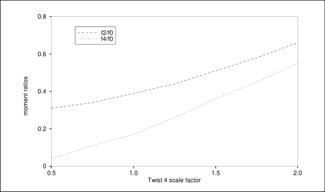
Figure 5: Sensitivity of moments to uniform rescaling of twist-4 terms

It was recently argued [8, 12] that there is no known rigorous argument to exclude the presence of an intrinsically nonperturbative $1/Q^{2}$ contribution to the coefficient function of the identity operator, and hence to the correlators $M_{n}(Q^{2})$ (this issue is intimately related with the location of the first infrared renormalon in the theory). In fact, if we return to the full logarithmic fits summarized in Table 1, and assume ignorance of the twist 2 terms by setting the coefficients $A_{n},B_{n}$=0, we find perfectly consistent fits to the duality Ansatz (40). It should be emphasized that the fitting procedure does not provide any internal evidence that important contributions are missing. Indeed, the quality of the fits (using rms deviation as a figure of merit) actually improves by almost an order of magnitude! And the optimal fits find the duality cut variable (which is allowed to float in the fitting procedure) $S_{n}$ settling at a self-consistent value, namely $\mu_{2}^{2}<S_{n}<\mu_{3}^{2}$ (since the lowest two mesons are included explicitly in the resonance sum part). The effect on the moments however is dramatic, and goes in the same direction as an increase in twist 4 contributions relative to lower twist terms discussed above. One now finds $f_{21}/f_{01}\simeq 1.0$ and $f_{41}/f_{01}\simeq 1.1$ implying a wavefunction with a minimum at $x=1/2$, rather than the correct convex and singly peaked result.

As regards the implications of our results for 4 dimensional QCD, it must be admitted that the prospects for a really firm nonperturbative resolution of the pion wavefunction seem rather dim at present. From the perspective of QCD sum rules, a reliable result would seem to depend on reasonably accurate uniform control over the correlators over a wide $Q^{2}$ range. First principles calculations starting from lattice QCD, on the other hand, also seem to introduce truncations of the theory which lead to potentially dangerous distortions of wave-function structure. Further calculations to study the systematic lattice errors in both correlators and moments on 4 dimensional (quenched) lattices of the size presently available are in progress.

7 Acknowledgements

A.D. acknowledges gratefully the support of the EKA Fund, Columbia University, and of the NSF through grant 93-22114. S.P. was supported in part through Department of Energy Grant No. DE-FG02-91ER40685. E.S. was supported in part through DFG contract Li519/2-1.

References

- [1] V.L. Chernyak and A.R. Zhitnitsky, Phys. Reports 112, 173(1984).
- [2] M.A. Shifman, A.I. Vainshtein, and V.I. Zakharov, Nucl. Phys. B147,385; 448; 519(1979).
- [3] S. Gottlieb and A. S. Kronfeld, Phys. Rev. Lett. 55, 2231(1985).
- [4] V. Anisovich, D. Melikhov, and V. Nikonov, St. Petersburg Institute of Nuclear Physics preprint hep-ph/9503473.
- [5] H.-N. Li and G. Sterman, Nucl. Phys. B382, 129 (1992); A. Radyushkin, “Pion wave function from QCD sum rules with nonlocal condensates, CEBAF-TH-94-13 (hep-ph/9406237).
- [6] J. Schwinger, Phys. Rev. 128, 2425,(1962).
- [7] G. ’t Hooft, Nucl. Phys. B75, 461(1974).
- [8] L. Brown, L. Yaffe, and C. Zhai, Phys. Rev. D46, 4712(1992).
- [9] I. Bars and M.B. Green, Phys. Rev. D17,537(1978).
- [10] E. Schnapka, “Validity of Relativistic Potential Models in Confining Theories”, Univ. of Pittsburgh M.S. Thesis, Aug. 1993.
- [11] C. Callan, N. Coote, and D.J. Gross, Phys. Rev. D13, 1649(1975).
- [12] A. Duncan and S. Pernice, Phys. Rev. D51, 1956(1995).
- [13] V.A. Novikov et al, Phys. Reports C41,1 (1978).
- [14] J. Gasser and H. Leutwyler, Phys. Reports 87, 79(1982).