SPIN, TWIST AND HADRON STRUCTURE
IN DEEP INELASTIC PROCESSES

Abstract

These notes provide an introduction to polarization effects in deep inelastic processes in QCD. We emphasize recent work on transverse asymmetries, subdominant effects, and the role of polarization in fragmentation and in purely hadronic processes. After a review of kinematics and some basic tools of short distance analysis, we study the twist, helicity, chirality and transversity dependence of a variety of high energy processes sensitive to the quark and gluon substructure of hadrons.

Notes for Lectures Presented at the

International School of Nucleon Structure

The Spin Structure of the Nucleon

Erice, 3 – 10 August 1995

Introduction

In recent years hadron spin physics has emerged as one of the most dynamic areas of particle physics. During the same period the field has got considerably more complicated. In times past only longitudinal asymmetries, that have simple parton model interpretations, attracted much attention; only dominant effects, that scale in the Bjorken limit, were experimentally accessible; and only relatively crude experimental data were available. Now interest has spread to transverse polarization asymmetries, subdominant effects, polarization effects in fragmentation and in purely hadronic processes. The aim of these lectures is to present an introduction to spin dependent effects at dominant and subdominant order in deep inelastic processes including deep inelastic scattering of leptons, $e^{+}e^{-}$ annihilation, and Drell-Yan processes. The methods can be extended relatively straightforwardly to other spin dependent effects in hard processes.

In a short set of lectures some detail and background must be sacrificed. As for background, I will assume that readers are familiar with the elementary parton model treatment of highly inelastic processes in the “infinite momentum frame”. Anyone who is not familiar with basic parton model ideas should consult standard textbook presentations. [1, 2, 3] Although I will have a lot to say about the parton model, it may look poorly motivated to someone who has not seen the ideas presented in their simplest form first. As for detail, I will mostly ignore the complications of QCD radiative corrections, normally included via the renormalization group. There are many excellent treatments including books by Collins[4], Muta [5] and most recently in a context particularly well suited to these lectures, by Roberts. [6] Of course radiative corrections and the momentum scale dependence they generate are central to the understanding of QCD. Some important aspects are covered in Al Mueller’s lectures in this volume. Here we will be interested in the classification of scattering amplitudes in terms of helicity, chirality, twist, etc. – a classification which is largely (but not entirely) independent of radiative corrections. In many cases the soft, $\,\mbox{ln}\,Q^{2}$ dependence they generate can be regarded as decorations of our primary results. Where this is not the case, I will try to warn the reader and refer to the appropriate literature.

The main question to be addressed here is: How can one classify and interpret the wide variety of spin dependent phenomena expected in hard processes? Which phenomena are displayed in which experiments? What are the selection rules enforced by the symmetries of QCD? Which phenomena dominate at large-$Q^{2}$, which are suppressed, and what is the physical origin of the suppression? In short, the object is to provide the background for both experimental and theoretical analysis of spin effects in hard processes. In contrast, I will resist almost entirely the temptation to speculate about the origins of spin effects based on models of hadron structure. These notes are not intended to be an introduction to the so-called “spin crisis” which grew out of the observation that only a small fraction of the nucleon’s spin is carried by the spin of quarks. Theorists will not find their own or my own favorite explanation of the spin crisis in these lectures. That is a subject for another school.

Certain predictions of perturbative QCD are admired for being very general and independent of the difficult details of hadron structure. Examples include the cross section for $e^{+}e^{-}\rightarrow$ hadrons, event shapes in $e^{+}e^{-}$ annihilation, the $\,\mbox{ln}\,Q^{2}$ dependence of deep inelastic structure functions, and the Gross-Llewellyn Smith and Bjorken Sum Rules. Studies of these processes provide essential tests of QCD. These will not be major topics here. I will assume that perturbative QCD is correct and use it as a sophisticated probe of the poorly understood dynamics of confinement. As we shall see, perturbative QCD is by now so well understood that it is possible to “tune” the probe to measure the nucleon expectation values of a variety of quark and gluon distributions and correlations within hadrons. Probes can be selected for spin, twist and flavor quantum numbers, and can be used either to analyze the structure of hadronic targets or reaction fragments. No other approach yields such well defined information about hadronic bound states. This information may help guide us to a better understanding of confinement from first principles.

Many aspects of these lectures are based on work performed in collaboration with Xiangdong Ji. The reader who wishes to explore subjects in greater depth should look at refs. [7, 8, 9, 10, 11, 12], as well as other references provided in the text. I would like to thank Xiangdong for the pleasure of this long collaboration. Thanks are also due to Matthias Burkardt, Gary Goldstein and Aneesh Manohar who collaborated on other projects related to this work. In addition I have benefited greatly from discussions with Guido Altarelli, Xavier Artru, Ian Balitsky, Vladimir Braun, Gerry Bunce, John Collins, Vernon Hughes, Gerd Mallot, Al Mueller, Richard Milner, John Ralston, Phil Ratcliffe, Klaus Rith, Jacques Soffer, and Linda Stuart.

These lectures grew out of talks at schools and conferences in the early 1990’s. A version presented at the 1992 Graduiertenkolleg of the Universities of Erlangen and Regensberg at Kloster Banz, Germany, was recorded by Drs. H. Meyer and G. Piller. The present version is based on a manuscript prepared by Drs. Meyer and Piller from their notes. I would like to thank them for the substantial work they undertook at that time. Subsequently I have edited, reformulated and expanded the notes, most recently for the Erice School on the Internal Spin Structure of the Nucleon.

1 Kinematics and other Generalities

The organizers of the school asked if I would briefly introduce the kinematic and dynamical variables common in the study of deep inelastic processes. So before getting down to the business of dynamics here is a short summary — the cogniscenti will certainly want to skip this section. Others, who may be familiar with less streamlined notation might wish at least to look at eqs. (1.14), (1.15), (1.21), and (LABEL:eq:spindepxsection). I hope students with less background in perturbative QCD will find this section useful.

1.1 Deep Inelastic Scattering

1.1.1 Basic Variables

Deep inelastic scattering (DIS) is the archetype for hard processes in QCD: a lepton — in practice an electron, muon or neutrino — with high energy scatters off a target hadron — in practice a nucleon or nucleus, or perhaps a photon — transferring large quantities of both energy and invariant squared-four-momentum. For charged leptons the dominant reaction mechanism is electromagnetism and one photon exchange is a good approximation. For neutrinos either $W^{\pm}$ (charged current) or $Z^{0}$ (neutral current) exchange may occur. The weak interactions of electrons may also be studied either by means of small parity violating asymmetries originating in $\gamma-Z^{0}$ interference, or by means of the charged current reaction $e^{-}\rightarrow\nu_{e}$.

We are primarily interested in experiments performed with polarized targets. Neutrino scattering experiments require far too massive targets for polarization to be a practical option, so we will ignore them, although $W$-exchange has been observed in $e^{-}p\rightarrow\nu_{e}+X$, at HERA,[13] and could be extended to a polarized target, at least in principle. Thus we are mainly limited to charged lepton scattering by one photon exchange. The kinematics is shown in fig. (1). The initial lepton with momentum $k$ and energy $E$ exchanges a photon of momentum $q$ with a the target with momentum $P$. Only the outgoing electron with momentum $k^{\prime}$ and energy $E^{\prime}$ is detected.

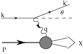
Figure 1: Kinematics of lepton-hadron scattering in the target rest frame

One can define the two invariants

$$q^{2}\equiv(k-k^{\prime})^{2}=q_{0}^{2}-\vec{q}\hskip 2.84526pt^{2}=-4EE^{\prime}\sin^{2}(\theta/2)=-Q^{2}<0$$ (1.1)

$$\nu\equiv P\cdot q=M(E-E^{\prime}),$$ (1.2)

where the lepton mass has been neglected (and will be neglected henceforth). The meaning of the scattering angle $\theta$ is clear from fig. (1). Unless otherwise noted, $E$, $E^{\prime}$, $\theta$ and $q^{0}\equiv E-E^{\prime}$ refer to the target rest frame. The deep inelastic, or Bjorken limit is where $Q^{2}$ and $\nu$ both go to infinity with the ratio, $x\equiv Q^{2}/2\nu$ fixed. $x$ is known as the Bjorken (scaling) variable.

Since the invariant mass of the hadronic final state is larger than or equal to the mass of the target, $(P+q)^{2}\geq M^{2}$, one has $0<x\leq 1$. It is convenient also to measure the energy loss using a dimensionless variable,

$$0\leq y\equiv{\nu\over ME}\leq 1.$$ (1.3)

We will find $E$, $Q^{2}$, $x$, and $y$ to be a useful set of variables. Note that it is overcomplete since $xy=Q^{2}/2ME$, and note also that what we define as $\nu$ differs from common usage by a factor of $M$. The behavior of cross sections at large $Q^{2}$ is much more transparent using these variables than using the set ($E,E^{\prime},\theta$) favored by experimenters for the reason that $\theta\rightarrow 0$ as $Q^{2}\rightarrow\infty$ at fixed $x$ and $y$.

1.1.2 Cross Section and Structure Functions

The differential cross-section for inclusive scattering ($eP\rightarrow e^{\prime}X$) is given by:

$$d\sigma={1\over J}{d^{3}k^{\prime}\over 2E^{\prime}(2\pi)^{3}}\sum_{X}\prod_{i=1}^{n_{X}}\int{d^{3}p_{i}\over(2\pi)^{3}2p_{i0}}|{\cal A}|^{2}(2\pi)^{4}\delta^{4}(P+q-\sum_{i=1}^{n_{X}}p_{i}).$$ (1.4)

The flux factor for the incoming nucleon and electron is denoted by $J=4P\cdot k$, which is equal to $J=4ME$ in the rest frame of the nucleon. The sum runs over all hadronic final states $X$ which are not observed. Each hadronic final state consists of $n_{X}$ particles with momenta $p_{i}$ ($\sum_{i=1}^{n_{X}}p_{i}\equiv p_{X}$). The squared-amplitude $|{\cal A}|^{2}$ can be separated into a leptonic ($l^{\mu\nu}$) and a hadronic ($W^{\mu\nu}$) tensor (see fig. (2)):

$$\left|{{\cal A}\over 4\pi}\right|^{2}={\alpha^{2}\over Q^{4}}l^{\mu\nu}W_{\mu\nu},$$ (1.5)

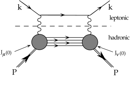
Figure 2: The squared amplitude ${\cal A}$ for electron-hadron scattering can be separated into a leptonic tensor $l^{\mu\nu}$ and a hadronic tensor $W^{\mu\nu}$.

where $\alpha\sim 1/137$ is the electromagnetic fine structure constant. The leptonic tensor $l^{\mu\nu}$ is given by the square of the elementary spin $1/2$ current (summed over final spins):

$$l^{\mu\nu} = \sum_{s^{\prime}}\bar{u}(k,s)\gamma^{\mu}u(k^{\prime},s^{\prime})\bar{u}(k^{\prime},s^{\prime})\gamma^{\nu}u(k,s)$$

$$= 2(k^{\prime\mu}k^{\nu}+k^{\prime\nu}k^{\mu})-2g^{\mu\nu}k\cdot k^{\prime}+2i\epsilon^{\mu\nu\lambda\sigma}q_{\lambda}s_{\sigma},$$

and consists of parts symmetric and antisymmetric in $\mu$ and $\nu$. The antisymmetric part is linear in the spin vector $s$, which is normalized to $s^{2}=-m^{2}$. While the leptonic tensor is known completely, $W^{\mu\nu}$, which describes the internal structure of the nucleon, depends on non-perturbative strong interaction dynamics. It is expressed in terms of the current $J^{\mu}$ as:

$$4\pi W^{\mu\nu} = \sum_{X}\langle PS|J^{\mu}|X\rangle\langle X|J^{\nu}|PS\rangle(2\pi)^{4}\delta(P+q-p_{X})$$ (1.7)

$$= \int d^{4}\xi e^{iq\cdot\xi}\langle PS|[J^{\mu}(\xi),J^{\nu}(0)]|PS\rangle_{c}.$$ (1.8)

The steps leading from eq. (1.7) to eq. (1.8) include writing the $\delta$ function as an exponential,

$$(2\pi)^{4}\delta^{4}(K)=\int d^{4}\xi e^{i\xi\cdot K},$$ (1.9)

translating the current, $e^{i\xi\cdot(P-p_{X})}\langle PS|J^{\mu}(0)|X\rangle=\langle PS|J^{\mu}(\xi)|X\rangle$, and using completeness, $\sum_{X}|X\rangle\langle X|=1$. Note that another term has been subtracted to convert the current product into a commutator. It is easy to check that the new term vanishes for $q^{0}>0$ which is the case for physical lepton scattering from a stable target. The subscript _c means that the graphs associated with the matrix element must be connected. Finally, note that the states are covariantly normalized to:

$$\langle P|P^{\prime}\rangle=2E(2\pi)^{3}\delta^{3}(P-P^{\prime}).$$ (1.10)

The optical theorem:

$$2\pi W^{\mu\nu}={\rm Im}\hskip 5.69054ptT^{\mu\nu}$$ (1.11)

relates the hadronic tensor to the imaginary part of the forward virtual Compton scattering amplitude, $T$:

$$T_{\mu\nu}=i\int d^{4}\xi e^{iq\cdot\xi}\langle PS|T(J_{\mu}(\xi)J_{\nu}(0))|PS\rangle$$ (1.12)

as shown graphically in fig. (3).

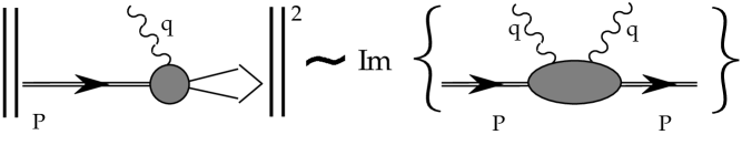
Figure 3: The optical theorem relates the hadronic structure tensor, $W^{\mu\nu}$ to the imaginary part of forward ($P=P^{\prime}$, $q=q^{\prime}$), virtual ($Q^{2}<0$) Compton scattering

1.1.3 Structure Functions

Using Lorentz covariance, gauge invariance, parity conservation in electromagnetism and standard discrete symmetries of the strong interactions, $W^{\mu\nu}$ can be parametrized in terms of four scalar dimensionless structure functions $F_{1}(x,Q^{2})$, $F_{2}(x,Q^{2})$, $g_{1}(x,Q^{2})$ and $g_{2}(x,Q^{2})$. They depend only on the two invariants $Q^{2}$ and $\nu$, or alternatively on $Q^{2}$ and the dimensionless Bjorken variable $x$. Splitting $W^{\mu\nu}$ into symmetric and anti-symmetric parts we have,

$$W^{\mu\nu}=W^{\{\mu\nu\}}+W^{[\mu\nu]},$$ (1.13)

with

$$W^{\{\mu\nu\}} = \left(-g^{\mu\nu}+{q^{\mu}q^{\nu}\over q^{2}}\right)F_{1}+\left[\left(P^{\mu}-{\nu\over q^{2}}q^{\mu}\right)\left(P^{\nu}-{\nu\over q^{2}}q^{\nu}\right)\right]{F_{2}\over\nu},$$ (1.14)

$$W^{[\mu\nu]} = -i\epsilon^{\mu\nu\lambda\sigma}q_{\lambda}\left({S_{\sigma}\over\nu}\left(g_{1}+g_{2}\right)-{q\cdot SP_{\sigma}\over\nu^{2}}g_{2}\right),$$ (1.15)

where $S^{\sigma}$ is the polarization vector of the nucleon $(S^{2}=-M^{2})$, $P\cdot S=0$. $S^{\sigma}$ is a pseudovector. Since $W^{[\mu\nu]}$ is a normal tensor, parity demands that the $S^{\mu}$ appear with another pseudotensor, and the only one available is the $\epsilon^{\mu\nu\sigma\lambda}$. Students often ask why $W^{\mu\nu}$ depends only linearly on $S^{\mu}$ – what is wrong with $S^{\mu}S^{\nu}$, for example? Lorentz invariance demands that $W^{\mu\nu}$, defined in eq. (1.8) be linear in the initial and final nucleon spinors, $U(P,S)$ and $\bar{U}(P,S)$. Tensors constructed from these are either spin independent ($\bar{U}(P,S)\gamma^{\mu}U(P,S)=2P^{\mu}$) or linear in $S^{\mu}$ (($\bar{U}(P,S)\gamma^{\mu}\gamma_{5}U(P,S)=2S^{\mu}$), but that is the end of it.

Note also that $W^{\mu\nu}$ is dimensionless (we shall have more to say about operator dimensions shortly). Factors of $\nu$ have been judiciously introduced into eqs. (1.15) and (1.14) so that the four structure functions, $F_{1}$, $F_{2}$, $g_{1}$, and $g_{2}$ are dimensionless. These structure functions are related to others in common use by:

$$W_{1}=F_{1},\quad W_{2}={M^{2}\over\nu}F_{2},\quad G_{1}={M^{2}g_{1}\over\nu},\quad G_{2}={M^{4}g_{2}\over\nu^{2}}.$$ (1.16)

1.1.4 Scaling and Kinematic Domains

Our choice of invariant structure functions makes the determination of scaling behavior at large $Q^{2}$ almost trivial. In the Bjorken limit where $Q^{2}\rightarrow\infty$ and $\nu\rightarrow\infty$, $x=Q^{2}/2\nu$ fixed, QCD becomes scale invariant up to logarithms of $Q^{2}$ generated by radiative corrections. Under a scale transformation, $P\rightarrow\lambda P$, $q\rightarrow\lambda q$, and $M\rightarrow\lambda M\neq M$, so a theory with a discrete spectrum of massive particles cannot be scale invariant except in a limit in which all masses are negligible. Thus no masses can appear in $W^{\mu\nu}$ in the Bjorken limit; it must be a dimensionless function of $P^{\mu}$, $q^{\mu}$, $S^{\mu}$, and the invariants $Q^{2}$ and $\nu$. In particular, it cannot depend explicitly on the target mass, $M$. If, for example, a term like ${{P^{\mu}P^{\nu}}\over M^{2}}W_{2}$ appeared in $W^{\{\mu\nu\}}$, it would violate scale invariance unless $W_{2}$ vanished like ${M^{2}\over\nu}$ at large $Q^{2}$. Clearly, the way to avoid such pathological choices of structure functions is to write the dimensionless tensor $W^{\mu\nu}$ in terms of dimensionless invariant functions using $\nu$ (or $Q^{2}$) to supply dimensional factors as needed. The immediate conclusion is that the functions $F_{1}$, $F_{2}$, $g_{1}$, and $g_{2}$ defined in eqs. (1.14) and (1.15), become functions only of the dimensionless ratio $x=Q^{2}/2\nu$, modulo logarithms, in the Bjorken limit,

$$F_{1}(Q^{2},\nu) \rightarrow F_{1}(x,\,\mbox{ln}\,Q^{2}),\quad F_{2}(Q^{2},\nu) \rightarrow F_{2}(x,\,\mbox{ln}\,Q^{2})$$

$$g_{1}(Q^{2},\nu) \rightarrow g_{1}(x,\,\mbox{ln}\,Q^{2}),\quad g_{2}(Q^{2},\nu) \rightarrow g_{2}(x,\,\mbox{ln}\,Q^{2})$$

as $Q^{2}$ and $\nu$ become large at fixed $x$. In practice it is observed that for $Q^{2}>1GeV^{2}$, the structure functions depend only very weakly on $Q^{2}$. Furthermore one observes an approximate relationship between $F_{1}$ and $F_{2}$, known as the Callan-Gross relation,[14]

$$F_{1}-{1\over 2x}F_{2}\sim{1\over\,\mbox{ln}\,Q^{2}},$$ (1.18)

which indicates that the particles that carry electric charge (the quarks) have spin ${1\over 2}$. The different kinematic domains of interest in inelastic electron scattering are shown in fig. (4).

Figure 4: Kinematic domains in electron-nucleon scattering.

1.1.5 Flavor Generalizations

Only up, down and strange quarks appear to be important constituents of light hadrons. The processes of interest to us, therefore are mediated by currents lying in the $SU(3)_{R}\times SU(3)_{L}$ space of $u,d,s$ vector and axial currents,

$$J_{\mu}^{a} \equiv{1\over 2}\bar{\psi}\gamma_{\mu}\lambda^{a}\psi,$$

$$J_{\mu 5}^{a} \equiv{1\over 2}\bar{\psi}\gamma_{\mu}\gamma_{5}\lambda^{a}\psi,$$

where $\lambda^{a}$ for $a=1,2\ldots 8$ are the flavor $SU(3)$ matrices, which are normalized to ${\rm Tr}\lambda^{a}\lambda^{b}=2\delta^{ab}$. Note, in particular, that $\lambda_{3}={\rm diag}(1,-1,0)$ and $\lambda_{8}={\rm diag}{1\over\sqrt{3}}(1,1,-2)$. In addition one has the flavor singlet current $J_{\mu}^{0}=\sqrt{2/3}\bar{\psi}\gamma_{\mu}\psi$, acting like $\sqrt{2\over 3}{\rm diag}(1,1,1)$ in flavor space.

1.1.6 Cross Section for Electron-Hadron Scattering

The differential cross section for unpolarized electron-hadron scattering can now be expanded in the Lorentz scalar structure functions by contracting the symmetric tensor, eq. (1.14), with the leptonic tensor, eq. (LABEL:lepten). Likewise the cross section for polarized scattering is obtained by contracting the antisymmetric tensor, eq. (1.15), with the same lepton tensor. The result is often quoted in terms of the experimenter’s variables, $Q^{2}$, $\nu$, $\theta$, $E$ and $E^{\prime}$, e.g. for the spin average case,

$${d^{3}\bar{\sigma}\over dE^{\prime}d\Omega}={4\alpha^{2}\over MQ^{4}}E^{\prime 2}\left\{2W_{1}(q^{2},\nu)\sin^{2}{\theta\over 2}+W_{2}(q^{2},\nu)\cos^{2}{\theta\over 2}\right\}.$$ (1.20)

The relative importance of the two terms is difficult to judge. Superficially it looks as though $W_{1}$ and $W_{2}$ are equally important. On second thought, $W_{1}$ is multiplied by $\sin^{2}{\theta\over 2}$ which gets small in the Bjorken limit. On third thought, $W_{2}$ vanishes like ${M^{2}\over\nu}$. To disentangle all this, we rewrite $d\bar{\sigma}$ in terms of $F_{1}$, $F_{2}$, $x$, $y$, and $Q^{2}$, where scaling behavior should be manifest,

$${d^{3}\bar{\sigma}\over dx\,dy\,d\phi}={e^{4}\over 4\pi^{2}Q^{2}}\left\{{y\over 2}F_{1}(x,Q^{2})+{1\over 2xy}\left(1-y-{y^{2}\over 4}(\kappa-1)\right)F_{2}(x,Q^{2})\right\}$$ (1.21)

with $\kappa\equiv 1-{4x^{2}M^{2}\over Q^{2}}$. No scaling approximations have been made in eq. (1.21). Under typical experimental conditions $y$ and $x$ are of order unity, though experiments are now being carried out at very low-$x$. Since $F_{1}\sim{1\over x}$ and $F_{2}\sim$ const. for small $x$, the two terms are comparable. There is no significant dependence on the azimuthal angle $\phi$, which cannot even be uniquely defined for inclusive scattering with an unpolarized target.

It is clear from the tensor structure of $\ell_{\mu\nu}$ and $W_{\mu\nu}$ that no target spin dependent effects survive if the beam is unpolarized. Therefore we lose no generality by defining the spin dependent cross section, $\Delta\sigma$ as half the difference between right- and left-handed incident electron cross sections,[15]

$${d\Delta\sigma(\alpha)\over dx\,dy\,d\phi} = {e^{4}\over 4\pi^{2}Q^{2}}\Biggl{\{}\cos\alpha\left\{\left[1-{y\over 2}-{y^{2}\over 4}(\kappa-1)\right]g_{1}(x,Q^{2})-{y\over 2}(\kappa-1)g_{2}(x,Q^{2})\right\}$$

$$- \sin\alpha\cos\phi\sqrt{(\kappa-1)\left(1-y-{y^{2}\over 4}(\kappa-1)\right)}\,\left({y\over 2}g_{1}(x,Q^{2})+g_{2}(x,Q^{2})\right)\Biggr{\}}$$

Now the azimuthal angle $\phi$ and the angle, $\alpha$, between the target spin $\hat{S}$ and the incident electron momentum, $\hat{k}$, make non-trivial appearances. These and other kinematic variables are defined in fig. (5). Note the following:

• $\alpha$ is the angle between the spin vector of the target $(\hat{S})$ and the incident electron beam $(\hat{k})$, not the virtual photon direction $(\hat{q})$.

• $\phi$ is the azimuthal angle between the plane defined by ${\vec{k}}$ and ${\vec{k}}^{\prime}$ and the plane defined by ${\vec{k}}$ and $\hat{S}$.

• Eqs. (1.21) and (LABEL:eq:spindepxsection) are exact (except that lepton masses have been ignored): no scaling limit has been taken. $\kappa-1\equiv M^{2}Q^{2}/\nu^{2}=4M^{2}x^{2}/Q^{2}$ is a measure of the approach to the scaling limit, $Q^{2}\to\infty$.

• To eliminate spin-independent effects one may either (i) subtract cross sections for different values of $\alpha$; (ii) subtract cross sections for right- and left-handed leptons; or (iii) measure $\phi$-dependence.

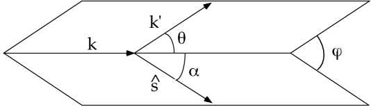
Figure 5: Kinematic variables in polarized lepton scattering from a polarized target.

Notice that effects associated with $g_{2}(x,Q^{2})$ are suppressed by a factor $\sqrt{\kappa-1}={2Mx\over\sqrt{Q^{2}}}$ with respect to the dominant structure function $g_{1}(x,Q^{2})$. In technical terms, this means that effects associated with $g_{2}$ are “higher twist” — suppressed by a power of $Q$ relative to the leading phenomena in the Bjorken limit. However, at $90^{\circ}$ the coefficient of the dominant term vanishes identically and allows the combination ${y\over 2}g_{1}+g_{2}$ to be extracted cleanly at large $Q^{2}$. This is a unique feature of the spin-dependent scattering. Only very rarely, to my knowledge, can a higher twist effect be selected by an adroit kinematic arrangement, thereby avoiding the difficult process of fitting and subtracting away a leading twist effect to expose the higher twist correction underneath.

1.2 Other Basic Deep Inelastic Processes

1.2.1 Inclusive $e^{+}$ $e^{-}$ Annihilation

In this process an electron with momentum $k$ and a positron with momentum $k^{\prime}$ annihilate to form a massive time-like photon with momentum $q=k+k^{\prime}$ ($Q^{2}\equiv q^{2}>0$), which decays into an unobserved final state. Through the optical theorem, the total cross section is proportional to the imaginary part of the photon propagator (see fig. (6)),

$$\sigma_{tot}={16\pi^{2}\alpha^{2}\over Q^{2}}\Pi(Q^{2}),$$ (1.23)

where $\Pi(Q^{2})$ is the Lorentz scalar spectral function appearing in the photon propagator:

$$\Pi_{\mu\nu}=(q_{\mu}q_{\nu}-q^{2}g_{\mu\nu})\Pi(Q^{2}),$$ (1.24)

and

$$\Pi(Q^{2})=-{1\over 6Q^{2}}\int d^{4}\xi e^{iq\cdot\xi}\langle 0|\left[J_{\mu}(\xi),J^{\mu}(0)\right]|0\rangle.$$ (1.25)

Figure 6: The optical theorem relates the total cross-section for $e^{+}e^{-}$ annihilation to the imaginary part of the photon propagator.

Usually the data are expressed as a ratio to the pointlike annihilation cross section to muons (to lowest order in $\alpha_{EM}$):

$$R(Q^{2})\equiv{\sigma_{tot}(e^{+}e^{-}\rightarrow hadrons)\over\sigma(e^{+}e^{-}\rightarrow\mu^{+}\mu^{-})}=12\pi\Pi(Q^{2}).$$ (1.26)

Since the hadronic process is initiated by the creation of a $q\bar{q}$ pair, $R$ directly measures the number of colors. At large $Q^{2}$ it is modified only by perturbative QCD corrections:

$$R(Q^{2}) = \sum_{q}3e_{q}^{2}\left\{1+{\alpha_{QCD}(Q^{2})\over\pi}+1.409{\alpha_{QCD}(Q^{2})\over\pi^{2}}-12.805{\alpha_{QCD}^{3}(Q^{2})\over\pi^{3}}+\cdots\right\}$$ (1.27)

$$+ \mbox{quark mass corrections}.)$$

The coefficients in eq. (1.27) are renormalization scheme dependent beyond lowest order. Those quoted in eq. (1.27) were calculated in $\overline{MS}$ scheme with five flavors.[16] The formula for $R$ does not depend on any details of hadronic structure, so it provides an important test of QCD (and measurement of $\alpha_{QCD}$). Similar remarks apply to processes in which jets are observed in the final state of $e^{+}e^{-}$ annihilation. Two jet events have the angular distribution that one expects for two spin $1/2$ quarks; a third jet is associated with gluonic bremsstrahlung. These processes however are not sensitive to the structure of hadrons and we will not discuss them further here.

1.2.2 Inclusive $e^{+}e^{-}$ Annihilation with One Observed Hadron

This process looks very much like a timelike version of deep inelastic scattering. Indeed it shares many important characteristics, but it also differs in essential ways. From the point of view of a theorist interested in hadron structure, the opportunity to study unstable hadrons makes this process very attractive. Deep inelastic scattering from $\Lambda$-hyperons or $\pi$ or $\rho$-mesons will never be more than a gedanken experiment. However, these and other unstable hadrons have already been studied in $e^{+}e^{-}$-annihilation. The physical basis of “fragmentation” — the process by which a quark created by the current from the vacuum fragments into the observed hadron — is not as well understood as DIS, making this an area of considerable interest at the present time.

The kinematics for $e^{+}e^{-}\rightarrow P+X$ is illustrated in fig. (7). Once again two kinematic invariants, $Q^{2}$ and $\nu=P\cdot q$, define the process. The limit of interest is $Q^{2},\nu\rightarrow\infty$, with $z\equiv{2\nu\over Q^{2}}$ fixed.

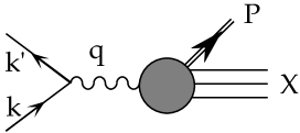
Figure 7: Kinematics for single particle inclusive annihilation — $e^{+}e^{-}\rightarrow PX$.

The momentum of the virtual photon is time-like, and that makes a major difference as we shall see in §2. The invariants are often expressed in terms of quantities measured in the $e^{+}e^{-}$ center of mass:

$$q^{2} \equiv Q^{2}=4E_{e}^{2}>0$$

$$P\cdot q \equiv \nu=E\sqrt{Q^{2}}$$

$$0<z \equiv {2P\cdot q\over q^{2}}={E\over E_{e}}\leq 1,$$

where E is the energy of the observed hadron. We shall usually be interested the polarization dependence, but here we illustrate the kinematics for the simpler, spin-averaged case. The cross section can be written as the product of a leptonic $\hat{l}_{\mu\nu}$ and a hadronic tensor $\hat{W}^{\mu\nu}$:

$$d\sigma\sim\hat{l}_{\mu\nu}\hat{W}^{\mu\nu}{d^{3}P\over(2\pi^{3})2E}$$ (1.29)

The hadronic tensor is determined by the electromagnetic current and depends on two invariant “fragmentation functions” due to current conservation and C, P and T invariance:

$$\hat{W}^{\mu\nu} = {1\over 4\pi}\sum_{X}(2\pi)^{4}\delta^{4}(P+P_{X}-q)\langle 0|J_{\mu}|PX\rangle_{\rm out\,\,out}\langle PX|J_{\nu}|0\rangle$$

$$= {1\over 4\pi}\int d^{4}\xi e^{iq\cdot\xi}\sum_{X}\langle 0|J_{\mu}(\xi)|PX\rangle_{\rm out\,\,out}\langle PX|J_{\nu}(0)|0\rangle$$

$$= -\left(g_{\mu\nu}-q_{\mu}q_{\nu}\over q^{2}\right)\hat{F}_{1}(z,q^{2})+{1\over\nu}\left(P_{\mu}-{\nu\over q^{2}}q_{\mu}\right)\left(P_{\nu}-{\nu\over q^{2}}q_{\nu}\right)\hat{F}_{2}(z,q^{2}).$$

In contrast to DIS, the sum over unobserved hadrons $X$ cannot be completed because the state $|PX\rangle_{\rm out}$ depends non-trivially on the observed hadron. Even if $P$ and $X$ did not interact, Bose or Fermi statistics prevents the states $X$ from being complete. In practice $P$ and $X$ interact dynamically, as indicated by the subscript “out”. For simplicity we will generally suppress this subscript. Thus, $e^{+}e^{-}\rightarrow P+X$ is not controlled by the product of two operators (electroweak currents), a feature which complicates the study of $e^{+}e^{-}\rightarrow P+X$ significantly.

If $q^{2}\rightarrow\infty$ at fixed $z$, the structure functions, $\hat{F}_{1}$ and $\hat{F}_{2}$ scale (up to logarithmic corrections) and obey a “Callan-Gross” relation, $\hat{F}_{1}+(z/2)\hat{F}_{2}\sim 1/\,\mbox{ln}\,q^{2}$. In this limit the cross section is:

$${d\sigma\over dzd\Omega}={\alpha^{2}\over Q^{2}}z\left\{\hat{F}_{1}(z,\,\mbox{ln}\,q^{2})+{1\over 4}z\sin^{2}\theta\hat{F}_{2}(z,\,\mbox{ln}\,q^{2})\right\}.$$ (1.31)

In leading logarithmic order, using “Callan-Gross”, the inclusive spectrum reduces to

$${1\over\sigma}{d\sigma\over dz}\sim{2\over R}z\hat{F}_{1}(z,q^{2})+\cdots,$$ (1.32)

where $R$ is defined by eq. (1.26).

1.2.3 Lepton Pair Production

The final process we will consider in detail is massive lepton-pair creation in hadron-hadron collisions – the so-called “Drell-Yan” process. The opportunities for study of novel aspects of hadron structure by means of polarized Drell-Yan experiments have motivated a major spin physics program at RHIC.[17] The kinematics of the lepton pair production are illustrated in fig. (8). Two hadrons with momenta $P$ and $P^{\prime}$ collide at a

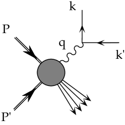
Figure 8: Kinematics of the Drell-Yan process.

center of mass energy $s=(P+P^{\prime})^{2}=4E_{CM}^{2}$. Two leptons with momenta $k_{1}^{\mu}$ and $k_{2}^{\mu}$ respectively are produced. They result from the decay of a timelike photon, $W^{\pm}$, or $Z^{0}$ carrying a momentum $q$, with $q^{2}=Q^{2}>0$. Two dimensionless scaling variables are defined by $x={2P\cdot q\over q^{2}}$ and $y={2P^{\prime}\cdot q\over q^{2}}$. It is easy to see that $xy=Q^{2}/s$. The differential cross section is

$$d\sigma\propto L_{\mu\nu}W^{\mu\nu}\frac{d^{3}k_{1}}{(2\pi)^{3}2k_{1}^{0}}\frac{d^{3}k_{2}}{(2\pi)^{3}2k_{2}^{0}}.$$ (1.33)

The decay of the virtual gauge boson is described by the leptonic tensor $L_{\mu\nu}$, whereas all information about the hadronic process are contained in $W^{\mu\nu}$:

$$W^{\mu\nu} = \frac{1}{2}s\sum\limits_{X}(2\pi)^{4}\delta^{4}(P+P^{\prime}-q-X)\phantom{\rangle}_{\rm in}\left<PP^{\prime}|J^{\mu}(0)|X\right>\left<X|J^{\nu}(0)|PP^{\prime}\right>_{\rm in}$$

$$= \frac{1}{2}s\int d^{4}\xi e^{-iq\cdot\xi}\phantom{\rangle}_{\rm in}\left<PP^{\prime}|J^{\mu}(\xi)J^{\nu}(0)|PP^{\prime}\right>_{\rm in},$$

where the in-state label on $|PP^{\prime}\rangle$ will usually be suppressed. $W^{\mu\nu}$ contains many Lorentz invariant structure functions $W_{k}$. Depending on the experimental circumstances different combinations of the $W_{k}$ and differential cross sections are of interest. As an example we consider the inclusive cross section where the lepton momenta have been integrated out, leaving $d\sigma/dq^{4}$,

$$\frac{d\sigma}{dq^{4}}=\frac{1}{6\pi^{3}}\frac{\alpha^{2}}{Q^{2}s^{2}}\left(-W_{\mu}^{\mu}\right).$$ (1.35)

The scaling limit ($s,Q^{2}\rightarrow\infty$ but $\tau\equiv Q^{2}/s$ fixed) once again yields a function of the dimensionless variables ($x$ and $y$) modulo logarithms induced by QCD radiative corrections, and in this case $W^{\mu}_{\mu}$ is of interest.

$$W_{\mu}^{\mu}\rightarrow W(x,y,\,\mbox{ln}\,{Q^{2}}).$$ (1.36)

2 Deep Inelastic Processes from a Coordinate Space Viewpoint

Traditional introductions to the parton model stay fixed in momentum space, where they use the device of the “infinite momentum frame” to simplify dynamical arguments. More sophistication is necessary to handle the complexities introduced by spin dependence and the subdominant effects associated with transverse spin in DIS. It is particularly useful to employ coordinate space methods, mixing parton phenomenology with somewhat more formal methods of the operator product expansion.[18] Certainly, sophisticated momentum space methods[19] can achieve the same results. However, it is particularly easy to distinguish and catalogue dominant and sub-dominant contributions using the operator product expansion in coordinate space.

In this section we will explore the coordinate space structure of the hard processes introduced in §1. Much of this material is to be found in modern field theory texts,[20] however there is an advantage to providing a brief, self-contained introduction which stresses only those elementary aspects of the formalism that are useful in characterizing deep inelastic spin physics.

2.1 $e^{+}e^{-}\rightarrow$ hadrons – The Short-distance Expansion

Inclusive $e^{+}e^{-}$ annihilation into hadrons is the simplest process to analyze and illustrates the importance of Wilson’s short distance expansion. As shown in §1, this process is described by the vacuum expectation value of a current commutator,

$$\Pi(Q^{2})\propto{1\over Q^{2}}\int d^{4}\xi\,e^{iq\cdot\xi}\left<0|\left[J_{\mu}(\xi),J^{\mu}(0)\right]|0\right>.$$ (2.1)

In the center of mass system we have $q=(\sqrt{Q^{2}},\vec{0}\,)$. Since the commutator is causal,

$$\left[J_{\mu}(\xi),J_{\nu}(0)\right]=0\quad{\rm for}\quad\xi^{2}<0,$$ (2.2)

then $|\vec{\xi}|<\xi^{0}$ in the integral. Using the symmetry of the commutator one obtains:

$$\Pi(Q^{2})\propto\int_{0}^{\infty}d\xi^{0}\sin{Q\xi^{0}}\int_{|\vec{\xi}|\leq\xi^{0}}d^{3}\xi\langle 0|\left[J_{\mu}(\xi),J^{\mu}(0)\right]|0\rangle$$ (2.3)

In the high energy limit, $Q\rightarrow\infty$, $\sin{Q\xi^{0}}$ oscillates rapidly, averaging out contributions except at the $\xi^{0}=0$ boundary of the integration region. This argument can be made more formal, leading to the conclusion that $\xi^{0}\sim{1\over q^{0}}$ gives the dominant contribution to the integral. Since $\xi^{0}>|\vec{\xi}|$ we can conclude that $e^{+}e^{-}$ annihilation into hadrons at high $Q^{2}$ is dominated by interactions at short distances, $\xi^{\mu}\rightarrow 0$. This is, of course, a Lorentz invariant condition.

The leading contribution to the annihilation process can now be found via the operator product expansion (OPE).[20] First postulated by Wilson, the existence of the OPE has been demonstrated to all orders in perturbation theory in renormalizable theories and also in various toy models which can be solved exactly. According to the OPE, a product of local operators $\hat{A}(\xi)$ and $\hat{B}(0)$ at short distances (here $\xi_{\mu}\rightarrow 0$) can be expanded in a series of non-singular local operators multiplying c-number singular functions,

$$\hat{A}(\xi)\hat{B}(0)\sim\sum\limits_{[\alpha]}C_{[\alpha]}(\xi)\hat{\theta}_{[\alpha]}(0)\quad{\rm as}\quad\xi^{\mu}\rightarrow 0.$$ (2.4)

In general the product $\hat{A}\hat{B}$ is singular as $\xi\rightarrow 0$. The substance of the expansion is that the singularities can be isolated in the c-number “Wilson coefficients”, $C_{[\alpha]}$. The operators in eq. (2.4) are cutoff independent renormalized operators and the Wilson coefficients are likewise cutoff independent.

The behavior of the Wilson coefficients at $\xi_{\mu}\rightarrow 0$ follows from dimensional analysis. In natural units, all quantities are measured in dimensions of mass to the appropriate power. For simplicity, if a quantity, $\theta$ has units $m^{d_{\theta}}$, we write $d_{\theta}=[\theta]$. This is a simple concept, not to be confused with more subtle ones like anomalous dimensions or scale dimensions.[21] The dimension of all operators of interest to us can be deduced from the fact that charge and action are dimensionless. Thus $[J^{\mu}]=3$ because $\int d^{3}xJ^{0}(x)=Q$. For the quark field $[\psi]={3\over 2}$ because the free Dirac action is $\int d^{4}x\bar{\psi}i\gamma\cdot\partial\psi+\ldots$, likewise for the gluon field strength $[G_{\mu\nu}]=2$. Since we normalize our states covariantly, $\langle P|P^{\prime}\rangle=2E(2\pi)^{3}\delta^{3}(\vec{P}-\vec{P}^{\prime})$, $[\langle P|P^{\prime}\rangle]=-2$. For the vectors $[P^{\mu}]=[S^{\mu}]=1$. We see that $W_{\mu\nu}$ is dimensionless, as reflected in the form of eqs. (1.14) and (1.15).

Dimensional consistency applied to the OPE requires,

$$[\hat{A}]+[\hat{B}]=[C_{[\alpha]}]+[\hat{\theta}_{[\alpha]}].$$ (2.5)

What can account for the dimensions of the singular function $C_{[\alpha]}$? If the operators $\hat{A}$ and $\hat{B}$ are finite in the $m_{\rm quark}\rightarrow 0$ limit, then powers of $m_{\rm quark}$ can only appear in the numerator of $C$. The renormalization scale, $\mu$, necessary to render the theory finite can only appear in logarithms (of the form $\,\mbox{ln}\,{(\mu\xi)}$) order by order in perturbation theory. This leaves the coordinate $\xi$ itself to absorb the dimensions.

$$C_{[\alpha]}(\xi)\sim\frac{1}{\xi^{[\hat{A}]+[\hat{B}]-[\hat{\theta}_{[\alpha]}]}}\left(\,\mbox{ln}\,^{\gamma_{\theta}}(\mu\xi)+\ldots\right)\quad{\rm as}\quad\xi\rightarrow 0.$$ (2.6)

The exponent $\gamma_{\theta}$ is the “anomalous dimension” of the operator $\theta$ generated by radiative corrections. Without minimizing the importance of these logarithms, we will usually ignore them and focus on the gross, power law, behavior required by dimensional analysis. For given operators $\hat{A}$ and $\hat{B}$ the leading contribution at short distances comes from that term in the OPE having the lowest operator dimension $[\hat{\theta}_{[\alpha]}]$.

This can now easily be applied to $e^{+}e^{-}$ annihilation. The dimension of the hadronic electromagnetic current is $[J_{\mu}]=3$. No fields have negative dimensions, so the lowest dimension operator is the unit operator, $\hat{\theta}_{0}\equiv{\bf 1}$, with $[{\bf 1}]=0$. The $C_{0}(\xi)\sim 1/\xi^{6}$ and the dominant contribution in the OPE is,

$$\left<0|\left[J_{\mu}(\xi),J^{\mu}(0)\right]|0\right>\sim\frac{1}{\xi^{6}},\quad\mbox{modulo logarithms}.$$ (2.7)

Consequently the current correlation function scales like

$$\Pi(Q^{2})\sim{1\over Q^{2}}\int d^{4}\xi\,e^{iq\cdot\xi}\frac{1}{\xi^{6}}\sim 1,$$ (2.8)

again modulo logarithms, and the cross section eq. (1.23) scales like:

$$\sigma\left(e^{+}e^{-}\rightarrow{\rm hadrons}\right)\sim\frac{1}{Q^{2}}.$$ (2.9)

The logarithms can be gathered together into powers of ${\alpha_{s}\over\pi}$ as anticipated in eq. (1.27). Of course, having made no attempt to derive the OPE or to study the effects of radiative corrections and renormalization in detail, the example of the total $e^{+}e^{-}$ annihilation cross section becomes rather trivial. Nevertheless it provides a useful introduction to the more complicated cases which follow.

2.2 $lp\rightarrow lX$ – The Light-Cone Expansion

Next we turn to deep inelastic scattering, which is characterized by two large invariants – $Q^{2}$ and $\nu$. As we shall see, such processes are dominated by physics close to the light-cone.

2.2.1 Light-Cone Coordinates and Formulation of Deep Inelastic Scattering

The four-momenta $P^{\mu}$ and $q^{\mu}$ can be used to define a frame and a spatial direction. Without loss of generality we can choose our frame such that $P^{\mu}$ and $q^{\mu}$ have components only in the time and $\hat{e}_{3}$ directions. It is helpful to introduce the light-like vectors

$$p^{\mu} = \frac{p}{\sqrt{2}}\,(1,0,0,1),$$

$$n^{\mu} = \frac{1}{\sqrt{2}p}\,(1,0,0,-1)$$

with $n^{2}=p^{2}=0$ and $n\cdot p=1$. Up to the scale factor $p$, the vectors $p^{\mu}$ and $n^{\mu}$ function as unit vectors along opposite tangents to the light-cone. They may be used to expand $P^{\mu}$ and $q^{\mu}$,

$$q^{\mu} = \frac{1}{M^{2}}\left(\nu-\sqrt{\nu^{2}+M^{2}Q^{2}}\right)p^{\mu}+\frac{1}{2}\left(\nu+\sqrt{\nu^{2}+M^{2}Q^{2}}\right)n^{\mu},$$ (2.11)

$$P^{\mu} = p^{\mu}+\frac{M^{2}}{2}n^{\mu},$$ (2.12)

In the Bjorken limit $q^{\mu}$ simplifies to

$$\lim_{Bj}q^{\mu}\sim\left(\nu+\frac{1}{2}M^{2}x\right)n^{\mu}-xp^{\mu}+{\cal O}\left({1\over Q^{2}}\right).$$ (2.13)

$p$ selects a specific frame. For example $p=M/\sqrt{2}$ yields the target rest frame, while $p\rightarrow\infty$ selects the infinite momentum frame. The decomposition along $p^{\mu}$ and $n^{\mu}$ is equivalent to the use of light-cone coordinates, which are defined as follows. An arbitrary four-vector $a^{\mu}=(a^{0},a^{1},a^{2},a^{3})$ can be rewritten in terms of the four components $a^{\pm}={1\over\sqrt{2}}(a^{0}\pm a^{3})$, and $\vec{a}^{\perp}=(a^{1},a^{2})$. In this basis, the metric $g_{\mu\nu}$ has non-zero components, $g_{+-}=g_{-+}=1$ and $g_{ij}=-\delta_{ij}$, so $a\cdot b=a^{+}b^{-}+a^{-}b^{+}-\vec{a}^{\perp}\cdot\vec{b}^{\perp}$. The transformation to light-cone components can be recast as an expansion in the basis vectors $p^{\mu}$ and $n^{\mu}$,

$$a^{\mu}=\left(\frac{\sqrt{2}a^{-}}{p}\right)p^{\mu}+\left(\sqrt{2}a^{+}p\right)n^{\mu}+a^{\perp\mu}.$$ (2.14)

With these preliminaries it is easy to find the space-time region which dominates the DIS. Consider the hadronic tensor $W^{\mu\nu}$ defined in eq. (1.8):

$$W^{\mu\nu}=\frac{1}{4\pi}\int d^{4}\,\xi e^{iq\cdot\xi}\left<P|\left[J^{\mu}(\xi),J^{\nu}(0)\right]|P\right>,$$ (2.15)

Take the Bjorken limit by keeping $P$ fixed and $q\rightarrow\infty$. Define

$$\xi^{\mu}\equiv\eta p^{\mu}+\lambda n^{\mu}+\xi^{\perp\mu},$$ (2.16)

we find in the Bjorken limit:

$$\lim_{Bj}q\cdot\xi=\eta\nu-x\lambda.$$ (2.17)

Arguments similar to those used in the previous section show that the integral in eq. (2.15) is dominated by $\eta\sim 1/\nu\sim 0$ and $\lambda\sim 1/x$, which is equivalent to $\xi^{-}\sim 0$ and $\xi^{+}\sim 1/xp$ respectively.[22, 23] As in the previous case the commutator in eq. (2.15) vanishes unless $\xi^{2}=2\lambda\eta-\vec{\xi}_{\perp}^{2}\geq 0$ because of causality. Combining these results we find that the Bjorken limit of DIS probes a current correlation function near the light-cone $\xi^{2}=0$, extending out to distances ($\xi^{3}$ and $\xi^{0}$) of order ${1\over{xp}}$.

2.2.2 Deep Inelastic Scattering and the Short Distance Expansion

QCD simplifies at short distances on account of asymptotic freedom. The analysis of $e^{+}e^{-}\rightarrow$ hadrons simplifies greatly for this reason. Deep inelastic scattering is not a short distance process; it is light-cone dominated. Nevertheless it can be related to the OPE and to short distances with considerable resulting simplification.

To show this we consider the so-called the Bjorken-Johnson-Low limit ($\lim_{BJL}$).[24, 25] This is a somewhat old fashioned method, mostly supplanted by Wilson’s operator product expansion. It has the virtue that the connection between measurable structure functions and local operators is extremely clear (via dispersion relations). Use of the BJL limit prevents one making mistakes in subtle cases.[26, 27] In the BJL limit one takes $\vec{q}=0$ and $q^{0}\rightarrow i\infty$, which yields $q^{2}\rightarrow-\infty$ and $x\rightarrow-i\infty$. In the physical region $x$ is restricted to be real and between $0$ and $1$. So the hadronic tensor $W_{\mu\nu}$ cannot be measured in the BJL limit. It is useful because 1) it is dominated by short distances, and 2) it can be related to $W_{\mu\nu}$ in the physical region through dispersion relations. Remember that $W_{\mu\nu}$ is the imaginary part of the forward, virtual Compton amplitude, $T_{\mu\nu}$, by the optical theorem,

$$T_{\mu\nu}(q^{2},\nu)=i\int d^{4}\xi\,e^{iq\cdot\xi}\left<P|T\left(J_{\mu}(\xi)J_{\nu}(0)\right)|P\right>,$$ (2.18)

For simplicity we suppress Lorentz indices and spin degrees of freedom for a while. Standard dispersion theory arguments show that $T(q^{2},\nu)$ is an analytic function of $\nu$ at fixed spacelike $q^{2}$ with branch points on the real–$\nu$ axis at $\nu=\pm{Q^{2}\over{2M}}$, the threshold for the elastic process $\gamma^{*}p\rightarrow\gamma^{*}p$. In fig. (9) one can see the physical region of this process and the area of the BJL limit in the complex $\omega=1/x$ plane. The physical cuts lie on the real axis from ${1\over x}=\pm 1$ to $\pm\infty$. This means that $T(q^{2},{1\over x})$ is analytic within the unit circle about the origin. The BJL limit takes $1\over x$ to zero along the imaginary axis. Thus $T(q^{2},\nu)$ can be expanded in a Taylor series in $({1\over x})$ about the origin in the BJL-limit.

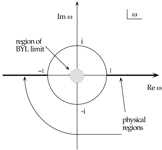
Figure 9: Physical region of the forward Compton amplitude and the BJL limit in the complex $\omega$ plane.

The coefficients in the Taylor expansion can be obtained from the dispersion relation obeyed by $T$. First remember that the optical theorem relates the imaginary part of $T$ to the hadronic tensor $W(q^{2},\nu)$ in the physical region,

$${\rm Im}T(q^{2},\nu)=4\pi W(q^{2},\nu).$$ (2.19)

Dispersion theory tells us that an analytic function can be represented in terms of its singularities in the complex plane,[28] in this case the physical cut on the real axis,

$$T(q^{2},\omega)=4\int_{1}^{\infty}d\omega^{\prime}\,\omega^{\prime}\,\frac{W(q^{2},\omega^{\prime})}{\omega^{\prime 2}-\omega^{2}}.$$ (2.20)

Crossing, i.e. $T(\omega)=T(-\omega)$, has been used. Since $T(q^{2},x)$ is analytic for $|{1\over x}|<1$ it may be expanded in a Taylor series in powers of ${1\over x}$:

$$\lim_{\rm BJL}T(q^{2},x)=4\sum\limits_{\rm n\,even}M^{n}(q^{2})\,{1\over x^{n}},$$ (2.21)

with

$$M^{n}(q^{2})=\int_{0}^{1}dxx^{n-1}W(q^{2},x).$$ (2.22)

Now consider where the BJL limit leads us in coordinate space. With $\vec{q}=0$ and $q^{0}\rightarrow i\infty$, the factor $e^{iq\xi}$ in eq. (2.18) reduces to $e^{-|q^{0}|\xi^{0}}$ and forces $\xi^{0}$ to zero. Although the time ordered product does not vanish outside the light-cone, it can be exchanged for a “retarded commutator”,[25, 26] which does. Thus $\xi^{0}\rightarrow 0$ forces $\xi^{\mu}\rightarrow 0$ and we conclude that the BJL-limit takes us to short distances where Wilson’s operator product expansion may be used. The OPE analysis of the product of currents yields a power series in ${1\over x}$ multiplying the matrix elements of local operators. Identifying terms in this Taylor series with the terms in eq. 2.21 we obtain the celebrated “moment sum rules” relating integrals over deep inelastic structure functions to target matrix elements of local operators. We will not pursue this direction further here — it is treated in standard references.[29, 20]

2.3 $e^{+}e^{-}\rightarrow h\,X$– Once Again, the Light-Cone

Like deep inelastic scattering, single particle inclusive production in $e^{+}e^{-}$ annihilation is dominated by the light-cone. However, the operator product expansion does not apply and no short distance analysis exists. The process is described by the tensor introduced in §1,

$$\bar{W}_{\mu\nu}=\frac{1}{4\pi}\int d^{4}\xi\,e^{iq\cdot\xi}\sum_{X}\left<0|J_{\mu}(\xi)|PX\right>\left<PX|J(0)_{\nu}|0\right>$$ (2.23)

Once again, the nucleon and photon momenta may be expanded in terms of the light-like vectors introduced in §2.2,

$$P^{\mu} = p^{\mu}+\frac{M^{2}}{2}n^{\mu},$$

$$q^{\mu} = \frac{1}{M^{2}}\left(\nu-\sqrt{\nu^{2}-M^{2}Q^{2}}\right)p^{\mu}+\frac{1}{2}\left(\nu+\sqrt{\nu^{2}-M^{2}Q^{2}}\right)n^{\mu},$$

and in the Bjorken limit ($Q^{2},\nu\rightarrow\infty$ with $z$ finite),

$$\lim_{Bj}q^{\mu}=\left(\nu-\frac{1}{2}{M^{2}\over z}\right)n^{\mu}+{1\over z}p^{\mu}.$$ (2.25)

It is traditional to use the photon rest frame ($\vec{q}=0,p\sim\sqrt{\nu}$) to analyze the process. However, the label on the state, ($P^{\mu}$) changes as the limit $Q^{2}\rightarrow\infty$ is taken in this frame, making it difficult to sort out the important regions of the $\xi$-integration. Things are simpler in a frame where $P$ is fixed, e.g. the rest frame of the produced hadron, where $p={M\over\sqrt{2}}$. In such a frame, the analysis of the fourier integral in eq. (2.23) proceeds exactly in the same way as for the electroproduction process of §2.2. With

$$\xi^{\mu}=\eta p^{\mu}+\lambda n^{\mu}+\xi^{\mu\perp}$$ (2.26)

we find in the Bjorken limit

$$\lim_{Bj}q\cdot\xi=\eta\nu-{\lambda\over z}.$$ (2.27)

So, $\nu\rightarrow\infty$ implies $\eta\rightarrow 0$ and $\lambda\sim z$, since $z$ is finite. So light-like separations $\xi^{\mu}\xi_{\mu}\sim 0$ dominate again unless unusual variations occur in the matrix elements

$$\sum\limits_{X}\left<0|J(\xi)|PX\right>\left<PX|J(0)|0\right>,$$ (2.28)

which will not happen in the frame where $P$ is independent of $Q^{2}$ and $\nu$. Also the frequencies associated with the states in the sum $\sum\limits_{X}|X\left>\right<X|$ know nothing about $Q^{2}$ and $\nu$, and will not spoil the argument. For a contrasting situation see the discussion of Drell-Yan in the following sub-section.

One can thus conclude that light-cone distances dominate fragmentation. However, in contrast to DIS the OPE cannot be applied here since the observed hadron state, $|P\rangle$ interferes with the attempt to complete the sum on $X$. Nevertheless nearly all of the QCD phenomenology developed for DIS can be carried over to this case, primarily using momentum space methods we will not discuss here.[30] In §6 we will see that the limitations on the coordinate space analysis do not prevent us from analyzing spin, twist and chirality in fragmentation.

2.4 $PP\rightarrow l^{+}l^{-}X$ – The Drell-Yan Process

Finally we consider the Drell-Yan process. Here the relevant hadronic tensor is (see §1):

$$W^{\mu\nu}=\frac{1}{2}s\int d^{4}\xi\,e^{iq\cdot\xi}\left<PP^{\prime}|J^{\mu}(\xi)J^{\nu}(0)|PP^{\prime}\right>.$$ (2.29)

It is simplest to consider the case where only the dilepton invariant mass distribution $d\sigma/dq^{2}$ is measured, though other observables behave similarly. ${d\sigma\over{dq^{2}}}$ depends only on $W^{\mu}_{\mu}$. We define a function, $W(s,Q^{2})$ by integrating $W^{\mu}_{\mu}$ over all $q^{\mu}$ with $q^{2}=Q^{2}$ and $q^{0}>0$,

$$W(s,Q^{2}) = \frac{1}{(2\pi)^{4}}\int_{R}d^{4}q\,\delta(q^{2}-Q^{2})(-g^{\mu\nu}W_{\mu\nu})\theta(q^{0}),$$

$$= -4\pi^{2}s\int_{R}d^{4}q\,\delta(q^{2}-Q^{2})\sum\limits_{X}(2\pi^{4})\delta^{4}(P+P^{\prime}-q-X)$$

$$\times \left<PP^{\prime}|J^{\mu}|X\right>\left<X|J_{\mu}|PP^{\prime}\right>.$$ (2.31)

The virtual photon’s momentum is integrated over all values consistent with the constraint $q^{2}=Q^{2}$ and conservation of energy, $\sqrt{Q^{2}}<q_{0}<(s+Q^{2})/2\sqrt{s}$, which defines the region $R$. If we introduce the function

$$\Delta_{+}^{R}(\xi,Q^{2})=\int_{R}\frac{d^{4}q}{(2\pi)^{3}}\,e^{-iq\cdot\xi}\delta(q^{2}-Q^{2})\theta(q_{0}),$$ (2.32)

then $W(s,Q^{2})$ can be written as

$$W(s,Q^{2})=-s\int d^{4}\xi\,\Delta_{+}^{R}(\xi,Q^{2})\left<PP^{\prime}|J^{\mu}(\xi)J_{\mu}(0)|PP^{\prime}\right>.$$ (2.33)

In the scaling limit ($Q^{2},s\rightarrow\infty,\tau=Q^{2}/s$ fixed) $\Delta_{+}^{R}(\xi,Q^{2})$ approaches a well-studied function of quantum field theory, the free field singular function, $\Delta_{+}(\xi,Q^{2}),$[31],

$$\Delta_{+}(\xi,Q^{2}) = \frac{1}{4\pi}\epsilon(\xi_{0})\delta(\xi^{2})-\frac{mi}{8\pi\sqrt{\xi^{2}}}\theta(\xi^{2})\left(N_{1}\left(Q\sqrt{\xi^{2}}\right)-i\epsilon(\xi_{0})J_{1}\left(Q\sqrt{\xi^{2}}\right)\right)$$ (2.34)

$$+ \frac{mi}{4\pi^{2}\sqrt{-\xi^{2}}}\theta(-\xi^{2})K_{1}\left(Q\sqrt{\xi^{2}}\right).$$

$\Delta_{+}(\xi,Q^{2})$ is singular on the light-cone and would select out light-cone contributions were it not for high frequency variations in the matrix elements. These can occur because the hadron momenta $P$ and $P^{\prime}$ cannot be kept fixed as $Q^{2}\rightarrow\infty$ ($s\approx 2P\cdot P^{\prime}>Q^{2}$) in any frame. Even in free field theory or the parton model the matrix element behaves like

$$\left<PP^{\prime}|J^{\mu}(\xi)J_{\mu}(0)|PP^{\prime}\right>\sim\int d\alpha\,d\beta\,e^{i\alpha P\cdot\xi+i\beta P^{\prime}\cdot\xi}f(\alpha,\beta),$$ (2.35)

where $f(\alpha,\beta)$ labels the momentum components of the partons that contribute to the current. To see that such variation can lead to contributions off the light-cone, consider a frame defined through the two vectors

$$p^{\mu} = p\,(1,0,0,1),$$

$$p^{\prime\mu} = \frac{s}{4p}\,(1,0,0,-1).$$

The hadron and photon momenta can be written as

$$P^{\mu} = p^{\mu}+\frac{M^{2}}{s}p^{\prime}{}^{\mu},$$

$$P^{\prime}{}^{\mu} = p^{\prime}{}^{\mu}+\frac{M^{2}}{s}p^{\mu},$$

$$q^{\mu} = yp^{\mu}+xp^{\prime}{}^{\mu},\quad\mbox{for}\;|q_{T}|\ll\sqrt{Q^{2}}.$$

With $\xi^{\mu}=\eta p^{\mu}+\lambda p^{\prime}{}^{\mu}+\xi_{\perp}^{\mu}$ the hadronic tensor eq. (2.29) is then equal to

$$W_{\mu}^{\mu}=\int d\lambda\,d\eta\,d^{2}\xi_{T}\,\int d\alpha\,d\beta\,f(\alpha,\beta)e^{i\frac{s}{2}[(\alpha-y)\lambda+(\beta-x)\eta]}.$$ (2.38)

Therefore the phases will cancel and the Drell-Yan process will escape from the light-cone if $\alpha\approx y=2q\cdot P^{\prime}/s$ and $\beta\approx x=2q\cdot P/s$. In §5 we will return to this process and see that such phases are generated in a natural way.

2.5 Dominant and Subdominant Diagrams

Guided by our understanding of the regions of coordinate space important for various deep inelastic processes, we can return to the more familiar world of Feynman graphs and learn which diagrams are likely to give dominant and subdominant contributions. The quarks that couple to electroweak currents propagate according to $S_{F}(\xi)$, the Feynman propagator. In coordinate space, $S_{F}(\xi)$ behaves like ${1\over\xi^{3}}$ at short distances (note $S_{F}(\xi)\sim\int d^{4}p{e^{ip\xi}\over{\gamma\cdot p-m}}$),

Interactions will not increase the singularity. For example, coupling a gluon to the propagating quark gives,

Generally speaking in renormalizable field theories, interactions on propagating lines do not increase the order of the short-distance or light-cone singularity by more than logarithmic terms beyond free field theory. This can be used as a guideline to estimate the importance of different perturbative diagrams for hard processes.

As a first example, consider $e^{+}e^{-}\rightarrow$ hadrons. The total cross section is proportional to the vacuum polarization of the photon propagator, whose leading contribution results from

the quark-antiquark loop fourier transformed, this ${\cal O}({1\over\xi^{6}})$ behavior generates a cross section which scales like ${1\over Q^{2}}$. Radiative corrections introduce logarithmic dependence on $\xi^{2}$, $\,\mbox{ln}\,\xi^{2}\mu^{2}$, where $\mu^{2}$ is the renormalization point, but they do not change the power of the singularity in a renormalizable theory. The renormalization group may be used to sum classes of diagrams giving modifications of the ${1\over\xi^{6}}$ behavior which go like powers of logarithms in an asymptotically free theory like QCD.

In deep inelastic scattering the leading contribution to the cross section or the forward Compton amplitude is shown in fig. (10). It dominates because the free quark propagator has the greatest possible light-cone singularity. The modifications shown in figs. (11-14) introduce only logarithmic modifications of the $\sim 1/\xi^{3}$ singularity. Renormalization group summation of leading $\,\mbox{ln}\,\xi^{2}$ dependence leads to powers of $\,\mbox{ln}\,\xi^{2}\mu^{2}$ but no change in the fundamental power singularity. All radiative corrections can be classified in the fashion outlined by figs. (11-14).

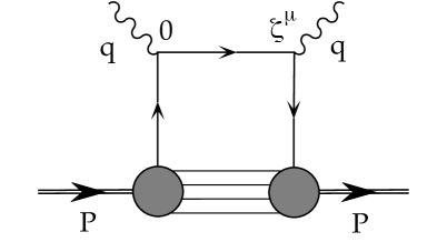
Figure 10: Leading diagram in deep inelastic scattering. The quark propagator between the two currents carries the large momentum $q^{\mu}$ and leads to a $1/\xi^{3}$ behavior at small distances.

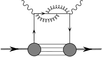
Figure 11: Radiative corrections to the quark propagator lead to $O\left(\alpha_{s}(\xi^{2})\right)$ corrections to the coefficient of the leading $1/\xi^{3}$ term.

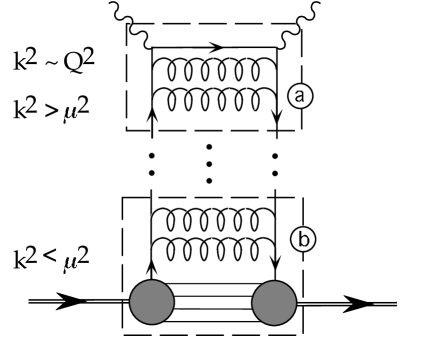
Figure 12: The higher order contributions in the upper part of the diagram $(a)$, where the quark virtuality is greater than $\mu^{2}$ lead to more $O\left(\alpha_{s}(\xi^{2})\,\,\mbox{ln}\,\mu^{2}\xi^{2}\right)$ corrections. The lower radiative corrections $(b)$ can be absorbed into the quark-hadron amplitude which will then depend on the renormalization scale $\mu^{2}$.

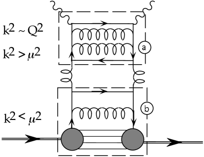
Figure 13: The upper part $(a)$ here generates a $c$-number coefficient function for gluonic operators in the product of two currents, beginning at $O\left(\alpha_{s}(\xi^{2})\,\,\mbox{ln}\,\mu^{2}\xi^{2}\right)$, while the lower part $(b)$ can be absorbed into a new gluon-hadron amplitude.

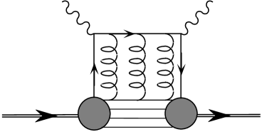
Figure 14: These corrections are either gauge artifacts or modifications of lower order in $1/\xi$.

For single particle inclusive $e^{+}e^{-}$ annihilation one finds in analogy to deep inelastic scattering the leading diagram fig. (15) which has a singularity $1/\xi^{3}$ from a propagating quark. Radiative corrections can be treated as before.

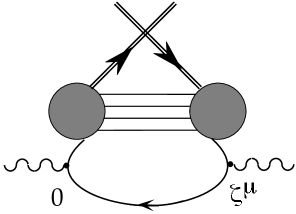
Figure 15: The dominant diagram for the single particle inclusive $e^{+}e^{-}$ annihilation.

If light-cone dominance were the only consideration, the diagram in fig. (16) would dominate the Drell-Yan process. However, if one studies the flow of hard momentum, this diagram turns out to be suppressed. The quark which brehmsstrahlungs the massive photon must be far off-shell, which is unnatural in a hadron-hadron collision. In coordinate space this is reflected by the fact that no large phases are generated by the matrix element.

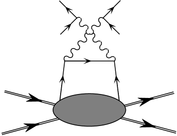
Figure 16: The diagram that has the leading light-cone singularity of the Drell-Yan process, but does not dominate.

The dominant contribution to the Drell-Yan process is shown in fig. (17).

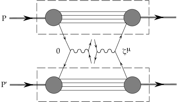
Figure 17: Dominant diagram of the Drell-Yan process.

The enclosed parts appear to be identical to the quark-hadron amplitude that occurs in the diagram that dominates in deep inelastic scattering. This means that at tree level, the same structure functions that appear in deep inelastic scattering also contribute to the Drell-Yan process. The diagram should still be dressed with QCD radiative corrections. The factorization theorem of QCD[32] says that this correspondence survives even in the presence of radiative corrections.

A subtlety of the Drell-Yan process is that the term most singular on the light-cone does not dominate, nevertheless the diagram gets its dominant contribution from $\xi^{2}\approx 0$. Returning to the definition of $W(Q^{2},s)$, we see that $\Delta_{R}(\xi,Q^{2})$ forces $\xi^{2}$ to zero, but the phase factors generated by the two separate quark-hadron amplitudes select tangent planes to the light-cone that contribute to the $\xi^{+}$ and $\xi^{-}$ integrals respectively.

One can now generalize these results to other processes, appealing to factorization.[32] For example fig. (18) shows the dominant contribution to one particle inclusive deep inelastic scattering in the current fragmentation region.

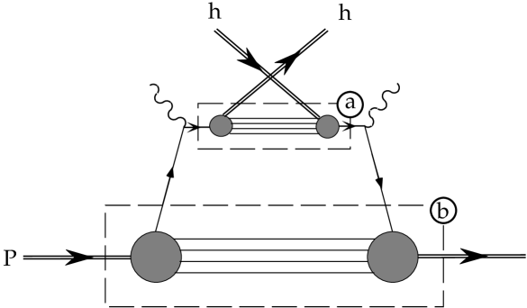
Figure 18: Dominant diagram for the one particle inclusive deep inelastic scattering.

Building blocks of these calculations are $(a)$ and $(b)$, defined and measured in $e^{+}e^{-}\rightarrow$ hadrons and DIS respectively. Factorization allows them to be carried from one process to another. They are the fundamental objects of study in hard inclusive QCD and command our attention.

3 Deep Inelastic Scattering and Generalized Distribution Functions I

In this first of two sections on deep inelastic scattering the focus will be on developing the tools necessary to perform a complete classification of effects at leading and next-to-leading order in ${1\over Q^{2}}$. We begin with some simple considerations of dimensional analysis, which we then apply to introduce the operator product expansion (OPE) and introduce the concept of “twist” which is useful to classify contributions to hard processes. To proceed further we must understand how to treat the Dirac structure of quark fields on the light-cone. This leads us briefly to explore light-cone quantization and introduce helicity, chirality and transversity as they apply to this problem. We will then look in some detail at a typical leading twist $({\cal O}(1))$ and next-to-leading twist $({\cal O}({1\over Q}))$ distribution before attacking the complete problem in §4.

3.1 Twist

In §2 we introduced the operator product expansion (OPE) as a tool for analyzing $e^{+}e^{-}\rightarrow{\rm hadrons}$, where the operator with lowest dimension dominates. We also argued that light-like distances ($\xi^{2}\sim 0$) dominate deep inelastic scattering. However, operators of high dimension can be important in this case. Instead a new quantum number, “twist”, related to both the dimension and spin of an operator, orders the dominant effects.

3.1.1 Twist and the OPE

As we learned in §2, the hadronic structure tensor of deep inelastic scattering,

$$4\pi W_{\mu\nu}=\int d^{4}\xi e^{iq\cdot\xi}\langle P,S|[J_{\mu}(\xi),J_{\nu}(0)]|P,S\rangle$$ (3.1)

is dominated by $\xi^{2}\sim 0$ in the $Q^{2}\rightarrow\infty$ limit. To make use of this, we expand the current commutator in terms of decreasing singularity around $\xi^{2}=0$,

$$\left[J(\xi),J(0)\right]\sim\sum_{[\theta]}K_{[\theta]}(\xi^{2})\xi^{\mu_{1}}\ldots\xi^{\mu_{n_{\theta}}}\theta_{\mu_{1}\ldots\mu_{n_{\theta}}}(0),$$ (3.2)

where $\theta_{\mu_{1}\ldots\mu_{n_{\theta}}}(0)$ are local operators, and $K_{[\theta]}(\xi^{2})$ are singular c-number functions that can be ordered according to their degree of singularity at $\xi^{2}=0$. Operators of the same singularity at $\xi^{2}=0$ will be of the same importance as $\xi^{\mu}\xi_{\mu}\rightarrow 0$ even though numerator factors of $\xi_{\mu}$ render some less singular than others as $\xi_{\mu}\rightarrow 0$. For simplicity we have suppressed all labels, including spin, on the currents $J(\xi)$. It often convenient (and sometimes essential) to regroup the terms in eq. (3.2) so that the operators $\theta_{\mu_{1}\ldots\mu_{n_{\theta}}}$ are traceless (i.e. $g^{\mu_{1}\mu_{2}}\theta_{\mu_{1}\ldots\mu_{n_{\theta}}}=0$, etc.) and symmetric in their Lorentz indices. We will assume this has been done.

Substituting the OPE into the definition of the structure function gives:

$$4\pi W=\int d^{4}\xi e^{iq\cdot\xi}\sum_{[\theta]}K_{[\theta]}(\xi^{2})\xi^{\mu_{1}}\ldots^{\mu_{n_{\theta}}}\langle P|\theta_{\mu_{1}\ldots\mu_{n_{\theta}}}(0)|P\rangle,$$ (3.3)

where the matrix elements have the form:

$$\langle P|\theta_{\mu_{1}\ldots\mu_{n_{\theta}}}(0)|P\rangle=P_{\mu_{1}}\ldots P_{\mu_{n_{\theta}}}M^{d_{\theta}-n_{\theta}-2}f_{\theta}+\ldots.$$ (3.4)

The $\ldots$ represent several types of terms which are less important in the Bjorken limit. We will return to them after looking at the dominant term.

Note that the power of a mass scale which appears in this expression is determined by dimensional analysis alone. We use the parameter $M$ generically for a typical hadronic mass scale $M\sim\Lambda_{QCD}\sim R^{-1}_{Bag}\sim M_{N}/3$. The power with which $M$ occurs defines the twist of the operator $\theta$,

$$t_{\theta}\equiv d_{\theta}-n_{\theta}$$ (3.5)

The degree of the light-cone singularity of $K_{[\theta]}\sim\xi^{-6+t_{\theta}}$ is also determined by dimensional analysis and depends only on the twist, $t_{\theta}$.

To carry out the fourier transformation make the substitution,

$$\xi^{\mu}\rightarrow-2iq^{\mu}{\partial\over\partial q^{2}}$$ (3.6)

which yields,

$$4\pi W\sim\sum_{\{\theta\}}\left({M\over\sqrt{q^{2}}}\right)^{t_{\theta}-2}\left({1\over x}\right)^{n_{\theta}}f_{\theta}$$ (3.7)

So the importance of an operator as $q^{2}\rightarrow\infty$ is determined by its twist. As we shall see, it is typical for towers of operators with the same twist (and other quantum numbers such as flavor) and increasing spin to appear in the OPE. Then it is convenient to sum over spin — $\sum_{n_{\theta}}f_{\theta}{1\over x}^{n_{\theta}}\equiv\tilde{f}_{\theta}(x)$ – where we now use the label $\theta$ to refer to the entire tower of operators.

The effect of radiative corrections is to introduce logarithmic dependence on $Q^{2}$ into the function $\tilde{f}_{\theta}$. Note however that the power law dependence on $Q^{2}$ is fixed by twist through dimensional analysis. Let us now return to the terms omitted in eq. (3.4). These include terms like $P_{\mu_{1}}\ldots P_{\mu_{n-2}}g_{\mu_{n-1}\mu_{n}}M_{N}^{2}$ that make the expression traceless. It is easy to see that these contribute at most corrections of order ${M_{N}^{2}\over Q^{2}}$ to the term we have kept. To carry through a complete analysis beyond order ${1\over Q}$ it is necessary to keep careful track of these terms. This, and the fact that interesting spin effects appear at ${\cal O}({1\over Q})$, are the reasons we do not consider ${\cal O}({1\over Q^{2}})$ here.

The lowest twist operator towers in QCD have $t_{\theta}=2$ and scale – modulo logarithms – in the Bjorken limit. This reflects the underlying scale invariance of the classical lagrangian. The matrix elements of higher twist operators, or the higher twist manifestations of twist-two operators are invariably signalled by the appearance of positive powers of mass in expressions analogous to eq. (3.4). Dimensional analysis then forces compensating factors of large kinematic invariants in the denominator, suppressing the contribution. The simple conclusion is that we can order the importance of effects in the deep inelastic limit simply by keeping track of masses we are forced to introduce into the numerators of parton-hadron amplitudes in order to maintain the correct dimensions.

3.1.2 Examples and a Working Redefinition of Twist

To make the preceding discussion clearer, here are some explicit examples from free field theories. These examples are not only pedagogical – the second one generates the leading twist effects in QCD up to logarithms. The light-cone singularities can be isolated easily. For the time ordered product of two scalar currents built from scalar fields, $J(\xi)=:\phi(\xi)\phi(\xi):$, one can use Wick’s theorem to show that,

$$T(J(\xi)J(0))=-2\Delta_{F}^{2}(\xi)+4i\Delta_{F}(\xi):\phi(\xi)\phi(0):+:\phi(\xi)\phi(\xi)\phi(0)\phi(0):\,,$$ (3.8)

where the normal ordering operation is sufficient to render the operator products finite (in free field theory) as $\xi\rightarrow 0$, and

$$\Delta_{F}(\xi)={i\over 4\pi^{2}}{1\over\xi^{2}-i\epsilon}$$ (3.9)

for a massless scalar field. To finally obtain the form of eq. (3.2), simply Taylor expand the bilocal operators –

$$:\phi(\xi)\phi(0):=\sum_{n}\xi_{\mu_{1}}\ldots\xi_{\mu_{n}}\,:\{\partial^{\mu_{1}}\ldots\partial^{\mu_{n}}\phi(0)\}\phi(0):$$ (3.10)

The current associated with a vector flavor symmetry of a fermion field is

$$J_{\mu}^{a}(\xi)=:\bar{\psi}(\xi){\lambda^{a}\over 2}\gamma_{\mu}\psi(\xi):.$$ (3.11)

Making use of the identity

$$[\bar{\psi}_{1}\psi_{1},\bar{\psi}_{2}\psi_{2}]=\bar{\psi}_{1}\{\psi_{1},\bar{\psi}_{2}\}\psi_{2}-\bar{\psi}_{2}\{\psi_{2},\bar{\psi}_{1}\}\psi_{1}$$ (3.12)

(because $\{\psi_{1},\psi_{2}\}=0$ in free field theory), and, for a massless field,

$$\{\psi(\xi),\bar{\psi}(0)\}={1\over 2\pi}\partial/\epsilon(\xi_{0})\delta(\xi^{2}),$$ (3.13)

one can now express the commutator of two currents in terms of bilocal operators:[33]

$$\left[J^{\mu a}(\xi),J^{\nu b}(0)\right] = -{1\over 4\pi}\left(\partial_{\rho}\epsilon(\xi_{0})\delta(\xi^{2})\right)\Big{[}d^{abc}S^{\mu\rho\nu\alpha}A^{c}_{\alpha}(\xi,0)-id^{abc}\epsilon^{\mu\rho\nu\alpha}S^{5c}_{\alpha}(\xi,0)$$ (3.14)

$$+ if^{abc}S^{\mu\rho\nu\alpha}S^{c}_{\alpha}(\xi,0)+f^{abc}\epsilon^{\mu\rho\nu\alpha}A^{5c}_{\alpha}(\xi,0)\Big{]},$$

where the Lorentz structure is split into a symmetric and an antisymmetric part according to:

$$\gamma^{\mu}\gamma^{\rho}\gamma^{\nu} = S^{\mu\rho\nu\alpha}\gamma_{\alpha}-i\epsilon^{\mu\rho\nu\alpha}\gamma_{\alpha}\gamma^{5},$$

$$S_{\mu\rho\nu\alpha} \equiv {1\over 4}{\rm Tr}\gamma_{\mu}\gamma_{\rho}\gamma_{\nu}\gamma_{\alpha}=g_{\mu\rho}g_{\nu\alpha}+g_{\mu\alpha}g_{\nu\rho}-g_{\mu\nu}g_{\alpha\rho},$$ (3.15)

and the flavor structure is split in a similar way:

$$\lambda^{a}\lambda^{b}=\left(d^{abc}\lambda^{c}+if^{abc}\lambda^{c}\right).$$ (3.16)

The symmetric and anti-symmetric vector and axial bilocal currents are defined by,

$$S/A^{[5]c}_{\alpha}\equiv\bar{\psi}(\xi){\lambda^{c}\over 2}\gamma_{\alpha}[\gamma^{5}]\psi(0)\pm\bar{\psi}(0){\lambda^{c}\over 2}\gamma_{\alpha}[\gamma^{5}]\psi(\xi)$$ (3.17)

Once again the form of eq. (3.2) is obtained by Taylor expanding the bilocal operators.

We have presented these formulas in their full complexity because they summarize the algebra of free quarks at short distances. All of the traditional results of the quark parton model applied to DIS (scaling relations, the Adler, Bjorken, Gross-Llewellyn Smith and other sum rules, the Callan Gross relation, etc.) can be obtained directly from these relations.[26]

The steps of first expanding the bilocal operators, then resumming the tower after fourier transformation are very inefficient. Clearly it should be possible to work directly with the bilocal operators. The twist content of a bilocal operator is somewhat more complicated than that of a local operator. Consider, for example, the bilocal current, $\bar{\psi}(0)\gamma^{\mu}\psi(\xi)$, which occurs in eq. (3.14). The operator has dimension three and, were it a local operator, it would have spin-one. In fact it sums an infinite tower of operators of increasing spin and dimension, with $t\geq 2$. For example at short distance one can write:

$$\bar{\psi}(0)\gamma^{\mu}\psi(\xi) = \bar{\psi}(0)\gamma^{\mu}\psi(0)+\xi_{\nu}\bar{\psi}(0)\gamma^{\mu}\partial^{\nu}\psi(0)+\ldots$$ (3.18)

$$\equiv J^{\mu}(0)+\xi_{\nu}\theta^{\mu\nu}(0)+\ldots.$$ (3.19)

$J^{\mu}(0)$ is traceless, symmetric and local and has twist-two. The operator $\theta^{\mu\nu}$ can be decomposed into a traceless operator and a “trace”:

$$\theta^{\mu\nu}=\left\{\theta^{\mu\nu}-{1\over 4}g^{\mu\nu}\theta^{\lambda}_{\lambda}\right\}+{1\over 4}g^{\mu\nu}\theta^{\lambda}_{\lambda}.$$ (3.20)

The first term is traceless, symmetric, with twist-two. The second operator has spin-$0$, hence its twist is four. Further terms in the Taylor expansion of the bilocal operator each yield a tower of local operators beginning at twist-two and increasing in steps of two.

Up to now we have used twist only in the sense in which it was originally introduced — $t_{\theta}=d_{\theta}-n_{\theta}$. In practice, twist is used in a less formal way, to denote the order in ${1\over Q^{2}}$ (modulo logarithms) at which a particular effect is seen in a particular experiment. If it behaves like $(1/Q^{2})^{p}$, then the object of interest is said to have twist $t=2+2p$. A traceless symmetric operator of twist $t$ will generate contributions that go like $(1/Q^{2})^{(2-t)}$, $(1/Q^{2})^{(4-t)}\ldots$ as we saw explicitly for the operator $\theta_{\mu\nu}$. Although the two meanings of twist do not coincide perfectly, both are in common use.

We will make a definition of the twist of an invariant matrix element of a light-cone bilocal operators, that determines the scaling behavior of the matrix element. Matrix elements of operators like e.g. $\bar{\psi}(0)\gamma_{\mu}\psi(\lambda n)$ are the basic building blocks of the description of hard processes in QCD. So we will call “twist” the order in ${M/Q}$ at which an operator matrix element contributes to deep inelastic processes. A few virtues of our working definition are a) that it is easily read off by inspection of matrix elements; b) that it directly corresponds to suppression in hard processes; and c) that effects we label twist-$t$ never enter hard processes with suppression less than $(M/Q)^{t-2}$. The twist we associate with the invariant matrix element of a specific bilocal operator can be determined simply by considering the powers of mass which must be introduced to perform a Lorentz-tensor decomposition of the matrix element. The powers of mass carry through the entire calculation to the end where each power is compensated by a power of $Q$ in the denominator. Twist-two results in no suppression, therefore $t-2$ is to be associated with the number of powers of mass introduced in the tensor decomposition of a matrix element.

The method is best explained by example. Consider the spin averaged matrix element of the bilocal current, $\bar{\psi}(\lambda n)\gamma^{\mu}\psi(0)$ on the light-cone,

$$\langle P|\bar{\psi}(\lambda n)\gamma^{\mu}\psi(0)|P\rangle=p^{\mu}f_{1}(\lambda)+n^{\mu}M^{2}f_{2}(\lambda),$$ (3.21)

where the factor of $M^{2}$ must be introduced because $[n^{\mu}]=-1$. The twist of the first term is two but, due to the appearance of the factor $M^{2}$, the twist of the second term is four. In a physical application we assert that the factor of $M^{2}$ will survive all manipulations and appear in the result compensated dimensionally by a factor of $1/Q^{2}$. Note that it is possible for $f_{1}$ to pick up multiplicative factors of $M^{2}/Q^{2}$ during a calculation. Twist tells us the leading, not the exclusive, $Q^{2}$ dependence of an invariant piece of a light-cone bilocal operator. As a second example, consider

$$\langle P|\bar{\psi}(\lambda n)\psi(0)|P\rangle=Me(\lambda).$$ (3.22)

$e(\lambda)$ has twist-three due to the factor $M$ which must be introduced to preserve dimensions. Finally, consider the matrix element of a gluonic operator

$$\langle P|G_{\mu}^{\phantom{\mu}\alpha}(\lambda n)G_{\alpha\nu}(0)|P\rangle=p_{\mu}p_{\nu}f_{1}(\lambda)+(p_{\mu}n_{\nu}+p_{\nu}n_{\mu})f_{2}(\lambda)M^{2}+n_{\mu}n_{\nu}f_{3}(\lambda)M^{4},$$ (3.23)

which has a twist content that can be worked out by the reader.

3.1.3 Spin and Twist

Counting twist in the case of polarized targets (or fragments) has an added complication. The Lorentz tensors which describe a hadron’s spin can appear in the Lorentz decomposition of matrix elements — their role in determining twist must be explained. The objects of interest in polarized scattering (or fragmentation) are forward scattering matrix elements on a null plane: $\langle P,\epsilon|\theta(\lambda n,0)|P,\epsilon\rangle$. The matrix elements are bilinear in $\epsilon$ and $\epsilon^{*}$, where $\epsilon$ and $\epsilon^{*}$ are the generalized spinors describing the target (Dirac spinors for spin $1/2$, polarization vectors for spin 1, etc.). The matrix element is a tensor function of $\epsilon$ and $\epsilon^{*}$. For spin-$1/2$ the only (non-trivial) tensors which can be built from $u\times\bar{u}$ are $\bar{u}\gamma^{\mu}u=2P^{\mu}$, a vector, and $\bar{u}\gamma^{\mu}\gamma_{5}u=2S^{\mu}$, an axial vector. We have already analyzed $P^{\mu}$ (it gets decomposed into $p^{\mu}$ and $n^{\mu}$). To expose the twist content of terms proportional to $S^{\mu}$, express it in terms of $p^{\mu}$ and $n^{\mu}$:

$$S^{\mu}=(S\cdot n)p^{\mu}+(S\cdot p)n^{\mu}+S_{\perp}^{\mu}.$$ (3.24)

Since $S\cdot p=-M^{2}S\cdot n/2$, it is clear that the second term contributes at twist-four. The transverse spin term is more subtle. Because we have chosen to normalize $S^{2}=-M^{2}$, $[S_{\perp}]=1$ and because there are no transverse momenta in the problem, $S^{\mu}_{\perp}$ contains a hidden factor of the target mass. At the end of the day this factor will manifest itself in a suppression by ${M\over Q}$. So we conclude that appearances of $S_{\perp}$ accompany twist-three distributions. An example is provided by:

$$\langle PS|\bar{\psi}(0)\gamma^{\mu}\gamma_{5}\psi(\lambda n)|PS\rangle=S\cdot n\ p^{\mu}g_{1}(\lambda)+S_{\perp}^{\mu}\ g_{T}(\lambda)+S\cdot p\ n^{\mu}g_{3}(\lambda).$$ (3.25)

According to dimensional analysis, $g_{1}$ is a twist-two object, $g_{T}$ has twist-three and $g_{3}$ is a twist-four function. When combined with the analysis of the following section, one finds that the function we have labeled $g_{1}$ is the scaling limit of the “$g_{1}$” defined in §1. Similarly, $g_{T}$ turns out to be $g_{1}+g_{2}$. We discard $g_{3}$ because we are not concerned with twist-four.

The same method of analysis can be extended to higher spins. For a spin-$1$ target, all polarization information is contained in the spin-density matrix $\eta_{\mu\nu}\equiv\epsilon_{\mu}\epsilon^{*}_{\nu}$, which contains scalar ($\epsilon^{*}\cdot\epsilon$), vector ($S_{\mu}\equiv{i\over M^{2}}\epsilon_{\mu\nu\alpha\beta}P^{\nu}\epsilon^{*\alpha}\epsilon^{\beta}$), and tensor ($\hat{\eta}_{\mu\nu}\equiv\epsilon^{*}_{\mu}\epsilon_{\nu}+\epsilon^{*}_{\nu}\epsilon_{\mu}+g_{\mu\nu}{M^{2}\over 2}$) polarization information. Note $[S^{\mu}]=1$ and $[\hat{\eta}_{\mu\nu}]=2$. To determine the twist of the associated distributions, $\eta$ must be projected along $p^{\mu}$, $n^{\mu}$ and transverse directions.[34] For even higher spins a multipole analysis is more streamlined.[35]

3.2 Dominant Diagram in Coordinate Space

As a final, and physically important example, we take the dominant diagram identified in §2 and use coordinate space methods to compute it. Since the quark that propagates between currents suffers no interactions (we are ignoring gluon radiative corrections here), we may use free field theory. Working out the commutator of free currents, we get

$$W^{ab}_{\mu\nu} = {1\over 4\pi}\int d^{4}\xi e^{iq\cdot\xi}\langle P,S|[J^{a}_{\mu}(\xi),J^{b}_{\nu}(0)]|P,S\rangle$$ (3.26)

$$= -\left({1\over 4\pi}\right)^{2}\int d^{4}\xi e^{iq\cdot\xi}\partial^{\rho}(\delta(\xi^{2})\epsilon(\xi^{0}))\left\{S_{\mu\rho\nu\alpha}d^{abc}\langle PS|A^{c\alpha}(\xi,0)|PS\rangle+\ldots\right\},$$

which corresponds to the handbag diagram of fig. (10). The $\ldots$ represent three more terms, given in eq. (3.14). This simple free-field picture is modified by:

• vertex and self energy corrections, which modify the singular function (fig. (11)). They give rise to logarithmic corrections, as do the dominant parts of

• ladder graphs (fig. (12)), and

• box graphs, which mix in gluons at ${\cal O}(\alpha_{s})$ (fig. (13)). Finally,

• in order to preserve color gauge invariance, one has to remember that the quark propagates in a gluon background (fig. (14)).

On account of the last point, the singular function of free field theory, $\{\psi(\xi),\bar{\psi}(0)\}={1\over 2\pi}\partial/\epsilon(\xi_{0})\delta(\xi^{2})$, must be changed to

$$\{\psi(\xi),\bar{\psi}(0)\}\rightarrow{1\over 2\pi}\partial/\epsilon(\xi_{0})\delta(\xi^{2}){\cal P}\left(\exp i\int_{0}^{\xi}d\zeta^{\mu}A_{\mu}(\zeta)\right),$$ (3.27)

which is the quark propagator in a background gluon field. [The path ordering (${\cal P}$) is necessary because $A_{\mu}(\zeta)$ is a matrix in color space.] The color field $A^{\mu}$ is that generated by remnants of the target nucleon and must be viewed as an operator sandwiched between the target hadron states. The bilocal operators in eq. (3.26) are therefore replaced by,

$$\bar{\psi}(\xi)\Gamma\psi(0)\rightarrow\bar{\psi}(\xi){\cal P}\left(\exp i\int_{0}^{\xi}d\zeta^{\mu}A_{\mu}(\zeta)\right)\Gamma\psi(0),$$ (3.28)

where $\Gamma$ stands for whatever color/flavor/Dirac matrices appear between $\bar{\psi}$ and $\psi$. The $\delta$-function in eq. (3.26) selects the light-cone. If we expand $\xi^{\mu}$ about the null plane, $\xi^{\mu}=\lambda n^{\mu}+\hat{\xi}^{\mu}$, it is easy to see that the terms involving $\hat{\xi}^{\mu}$ are twist-four and higher. One therefore has:

$$\langle PS|\bar{\psi}(0){\cal P}\left(\exp-i\int_{0}^{\xi^{\mu}}d\zeta^{\mu}A_{\mu}(\zeta)\right)\psi(\xi)|PS\rangle =$$

$$\langle PS|\bar{\psi}(0){\cal P}\left(\exp-i\int_{0}^{\lambda}d\tau n\cdot A(\tau n)\right)\psi(\lambda n)|PS\rangle + \ldots,$$ (3.29)

where the $\ldots$ represent the parts that vanish on the light-cone and have a twist $\geq 4$. In the light-cone gauge $n\cdot A=0$, explicit reference to gluons disappears. However, the inclusion of the “Wilson link”, ${\cal P}\left(\exp i\int_{0}^{\xi}d\zeta^{\mu}A_{\mu}(\zeta)\right)$, is essential in generating higher twist ($t\geq 4$) gluon corrections.

In the unpolarized case, the twist expansion of the bilocal operator matrix element gives

$$\int{d\lambda\over 2\pi}e^{i\lambda x}\langle P|\bar{\psi}_{a}(0)\gamma_{\mu}\psi_{a}(\lambda n)|P\rangle\equiv 2f_{1a}(x)p_{\mu}+2M^{2}f_{4a}(x)n_{\mu}$$ (3.30)

and, carrying out the fourier transform in eq. (3.26), we find

$$F_{1}(x)={1\over 2}\sum_{a}e_{a}^{2}(f^{a}_{1}(x)-f^{a}_{1}(-x)),$$ (3.31)

where $a=u,d,s,\ldots$ is the flavor index. The interpretation in terms of the parton model will be given later in this section.

A brief summary to this point is: Up to and including twist-three the basic objects of analysis in DIS are forward matrix elements of bilocal products of fields on the light-cone and in light-cone gauge,

$$\Gamma(x)=\int{d\lambda\over 2\pi}e^{i\lambda x}\langle PS|\bar{\psi}(0)\Gamma\psi(\lambda n)|PS\rangle.$$ (3.32)

Remember, that important $\,\mbox{ln}\,Q^{2}$ radiative corrections have been ignored in pursuit of the twist and spin dependence.

3.3 Learning from Light-Cone Quantization

Since the dominant contribution to DIS comes from the light-cone, it is natural to consider a dynamical formulation in which the light-cone plays a special role. At the birth of deep inelastic physics it was recognized that field theories simplify in some important ways if they are quantized “on the light-cone” rather than at equal times.[36, 37] Unfortunately some features which are simple at equal times become difficult on the light-cone. Certainly, as we shall see, there is much insight to be gained by considering deep inelastic processes using light-cone quantization. The larger question – whether QCD simplifies in essential ways when quantized on the light-cone – will not be pursued here.

Field theories may be quantized by imposing canonical equal-time commutation (or anticommutation) relations on the dynamically independent fields.[20] Lorentz invariance requires that any other space-like hyperplane in Minkowski space would serve as well as $\xi^{0}=0$. A null-plane, such as $\xi\cdot n=0$ is the limit of a sequence of space-like surfaces, and includes points that are causally connected. Although a field theory quantized on at $\xi\cdot n=0$ could differ from one quantized at $\xi^{0}=0$, they coincide for all examples of which I am aware. Let us study what happens if we attempt to quantize fermions on the surface $\xi^{+}=0$.[38] First we must introduce and familiarize ourselves with the unusual kinematics of the light-cone.

3.3.1 Light-Cone Kinematics

We have previously introduced light-cone coordinates $\xi^{\pm}={1\over\sqrt{2}}(\xi^{0}\pm\xi^{3})$ and $\vec{\xi}^{\perp}=(\xi^{1},\xi^{2})$, and the metric $g_{\mu\nu}$, with $g_{+-}=g_{-+}=1$, and $g_{ij}=-\delta_{ij}$. The partially off-diagonal structure of $g$ makes raising and lowering indices confusing, viz., $a^{+}=a_{-}$, and so forth. So we work with upper (contravariant) indices as much as possible.

Quantizing at (say) $\xi^{+}=0$, we are committed to $\xi^{+}$ as our evolution variable (just as quantization at $\xi^{0}=0$ fixes $\xi^{0}$ as the “time”). $\xi^{-}$ and $\xi^{\perp}$ are therefore kinematic, not dynamical variables. The conjugate momenta $p^{+}$ and $\vec{p}^{\perp}$ parameterize the fourier decomposition of the independent light-cone fields, just like $\vec{p}$ in ordinary quantization. $p^{-}$ is the “Hamiltonian” for light-cone dynamics.

3.3.2 Dirac Algebra on the Light-Cone

The usual selection of $\gamma^{0}={\rm diag}(1,1,-1-1)$ is prejudiced toward equal time quantization. Then a (anti-) particle at rest has only (“lower”) “upper” components in its Dirac spinor. Much of our analysis is simplified by choosing a representation for the Dirac matrices tailored to the light-cone.[38] To represent Dirac matrices compactly, we use the “bispinor” notation: let ($\sigma^{1},\sigma^{2},\sigma^{3}$) and ($\rho^{1},\rho^{2},\rho^{3}$) be two copies of the standard ($2\times 2$) Pauli matrices. A $4\times 4$ Dirac matrix can be represented as $\rho^{i}\otimes\sigma^{j}$. $\rho$ controls the upper-versus-lower two-component space; $\sigma$ controls the inner two-component space. An example will clarify the notation: the Dirac-Pauli representation used, for example, by Bjorken and Drell is,

$$\gamma^{0}_{BD} = \rho^{3}\otimes 1=\pmatrix{1&0\cr 0&-1}$$

$$\gamma^{j}_{BD} = i\rho^{2}\otimes\sigma^{j}=\pmatrix{0&\sigma^{j}\cr-\sigma^{j}&0}$$

$$\gamma^{5}_{BD} = \rho^{1}\otimes 1=\pmatrix{0&1\cr 1&0}$$

The light-cone representation useful for us is instead,

$$\gamma^{0} = \rho^{1}\otimes\sigma^{3}=\pmatrix{0&\sigma^{3}\cr\sigma^{3}&0}$$

$$\vec{\gamma}^{\perp} = 1\otimes i\vec{\sigma}^{\perp}=\pmatrix{i\vec{\sigma}^{\perp}&0\cr 0&i\vec{\sigma}^{\perp}}$$ (3.34)

$$\gamma^{3} = -i\rho^{2}\otimes\sigma^{3}=\pmatrix{0&-\sigma^{3}\cr\sigma^{3}&0}$$

$$\gamma^{5} = \rho^{3}\otimes\sigma^{3}=\pmatrix{\sigma^{3}&0\cr 0&-\sigma^{3}},$$

where $\perp\,=1\,{\rm or}\,2$. It is easy to check that eq. (LABEL:eq:mygamma) satisfy the usual algebra, $\{\gamma^{\mu},\gamma^{\nu}\}=2g^{\mu\nu}$, and $\gamma^{5}=i\gamma^{0}\gamma^{1}\gamma^{2}\gamma^{3}$.

Operators which project on the upper and lower two component subspaces play a central role in light-cone dynamics. Define ${\cal P}_{\pm}$ by,

$${\cal P}_{\pm} = {1\over 2}\gamma^{\mp}\gamma^{\pm}={1\over 2}(1\pm\alpha_{3})$$

$$\gamma^{\pm} = {1\over\sqrt{2}}(\gamma^{0}\pm\gamma^{3}),$$

with the properties:

$${\cal P}_{-}{\cal P}_{+} = {\cal P}_{+}{\cal P}_{-}=0$$

$${\cal P}_{\pm}^{2} = {\cal P}_{\pm}$$

$${\cal P}_{-}+{\cal P}_{+} = 1$$

$${\cal P}_{+}=\pmatrix{1&0\cr 0&0} {\cal P}_{-}=\pmatrix{0&0\cr 0&1}$$

The “light-cone projections” of the Dirac field, $\psi_{+}\equiv{\cal P}_{+}\psi$ and $\psi_{-}\equiv{\cal P}_{-}\psi$ are known as the “good” and “bad” light-cone components of $\psi$ respectively. To save on subscripts we shall frequently replace $\psi_{\pm}$ as follows,

$$\psi_{+}\Rightarrow\phi\quad\psi_{-}\Rightarrow\chi$$ (3.38)

3.3.3 Independent Degrees of Freedom

The importance of ${\cal P}_{\pm}$ becomes clear when they are used to project the Dirac equation down to two two-component equations,

$$i\gamma^{-}D_{-}\chi = -\vec{\gamma}^{\perp}\cdot\vec{D}^{\perp}\phi+m\phi$$

$$i\gamma^{+}D_{+}\phi = -\vec{\gamma}^{\perp}\cdot\vec{D}^{\perp}\chi+m\chi,$$ (3.39)

where $D_{\pm}={\partial\over{\partial\xi^{\pm}}}-igA^{\mp}$. In the light-cone gauge $A^{+}=0$. $\xi^{+}$ is the evolution (“time”) parameter, but the first of eq. (3.39) only involves $\partial/\partial\xi^{-}$, so it appears that $\chi$ is not an independent dynamical field. Instead the Dirac equation constrains $\chi$ in terms of $\phi$ and $\vec{A}_{\perp}$ at fixed $\xi^{+}$,

$$i\gamma^{-}{\partial\over{\partial\xi^{-}}}\chi=-\vec{\gamma}^{\perp}\cdot\vec{D}^{\perp}\phi+m\phi$$ (3.40)

The longitudinal component of the electric field in electrodynamic is similarly constrained (i.e. determined at any time) by Gauss’s Law in Coulomb gauge, $\vec{\nabla}\cdot\vec{E}=\rho$. Study of the gluon equations of motion indicates that $A^{-}$ is also a constrained variable. The independent fields are therefore $\phi$ and $\vec{A}_{\perp}$. $\chi$ should be regarded as composite — as specified by eq. (3.40) — $\chi={\cal F}[\phi,\vec{A}_{\perp}]$.

By the way, the reduction of the four-component Dirac field to two propagating degrees of freedom is not unique to light-cone quantization. In the usual treatment of the Dirac equation one finds only two solutions for each energy and momentum, corresponding to the two spin states of a spin-$1/2$ particle. The two-degrees of freedom corresponding to the antiparticle are found in the solution with energy $-E$ and momentum $-\vec{p}$. In fact, the Dirac equation in momentum space is literally written in the form of a projection operation, $\Lambda_{-}\psi=0$, where $\Lambda_{\pm}={1\over 2m}(p/\pm m)$ projects out two of the four components of the Dirac spinor.

Although the complete quantization of QCD requires much more work, the implication for the Dirac field is already clear: the good components should be regarded as independent propagating degrees of freedom; the bad components are dependent fields – actually quark-gluon composites.

The classification of quark spin states depends on the Dirac matrices which a) commute with ${\cal P}_{\pm}$ and b) commute with one-another. Returning to eq. (LABEL:eq:mygamma) we see that $\gamma^{1},\gamma^{2}$, and $\gamma_{5}$ commute with ${\cal P}_{\pm}$. Furthermore, the component of the generator of spin-rotations along the $\hat{e}_{3}$-direction,

$$\Sigma^{3}\equiv{i\over 2}[\gamma^{1},\gamma^{2}]=\pmatrix{\sigma^{3}&0\cr 0&\sigma^{3}},$$ (3.41)

also commutes with ${\cal P}_{\pm}$. Note that for a Dirac particle with momentum in the $\hat{e}_{3}$-direction, $\Sigma^{3}$ measures the helicity. This set of operators suggests two different maximal sets of commuting observables:

• Diagonalize $\gamma_{5}$ and $\Sigma^{3}$ — a chirality or helicity basis, or

• Diagonalize $\gamma^{1}$ (or equivalently, $\gamma^{2}$) – a transversity basis.

Let us consider these in turn –

Helicity Basis

In the helicity basis, both the good and bad components of $\psi$ carry helicity labels – the eigenvalues of $\Sigma^{3}$,

$$\psi=\pmatrix{\phi_{+}\cr\phi_{-}\cr\chi_{+}\cr\chi_{-}}.$$ (3.42)

Note that upper and lower components of $\psi$ correspond to good and bad light-cone components respectively. Referring back to the form of $\gamma_{5}$, eq. (LABEL:eq:mygamma), we see that helicity and chirality are identical for the good components of $\psi$ but opposite for the bad components,

$$\gamma_{5}\psi=\pmatrix{+\phi_{+}\cr-\phi_{-}\cr-\chi_{+}\cr+\chi_{-}}.$$ (3.43)

This may look strange at first, but it follows immediately from the composite nature of $\chi$. A quantum of $\chi$ with positive helicity is actually a composite of a transverse gluon and a quantum of $\phi$. Since the gluon carries helicity-one (but no chirality), angular momentum conservation requires that the $\phi$-quantum have negative helicity and therefore negative chirality. Remembering this association will help sort out the chirality and helicity selection rules which appear in the following sections.

Transversity Basis

Alternatively, we can diagonalize one of the transverse $\gamma$-matrices, to be specific, $\gamma^{1}$. We define eigenstates of the transverse spin-projection operators, ${\cal Q}_{\pm}={1\over 2}(1\mp\gamma_{5}\gamma^{1})$, (which commute with ${\cal P}_{\pm}$),

$${\cal Q}_{+}\phi \equiv \phi_{\perp}$$ (3.44)

$${\cal Q}_{-}\phi \equiv \phi_{\top},$$ (3.45)

and similarly for $\chi$. Of course $\phi_{\top/\perp}$ are linear combinations of $\phi_{\pm}$. Note however that $\phi_{\top/\perp}$ are not eigenstates of the transverse spin operator $\Sigma^{1}=\pmatrix{0&i\sigma^{1}\cr i\sigma^{1}&0}$, which is not diagonal in the basis of good and bad components of $\psi$. So we have to be careful that we do not carelessly confuse transversity, the quantum number associated with ${\cal Q}_{\pm}$, which is simple in this picture, with transverse spin, which is not.

3.4 The Parton Model

Following the path we are on, the parton model is merely the light-cone Fock space decomposition of the matrix elements which control hard processes. Since we have both the matrix elements and the Fock space in hand, it is straight-forward to construct the parton model. We will verify that the parton interpretation emerges as expected for twist-two and then explore twist-three. The reader should beware that twist-four is considerably more complicated. A parton model picture of twist-four does exist, however much work is required to make it obvious.[39, 19, 40]

The Fock space in the two bases can be constructed by defining operators that create the appropriate components of $\phi$. In the helicity basis we define $R^{\dagger}(k^{+},\vec{k}_{\perp})$ to create a right-handed (positive helicity) component of $\phi$ and $L^{\dagger}(k^{+},\vec{k}_{\perp})$ to create a left-handed (negative helicity) component of $\phi$, and $R^{\dagger}_{c}$ and $L^{\dagger}_{c}$, which do the same for the antiparticle field $\phi_{c}$. In the transversity basis we define the operators $\alpha^{\dagger}(k^{+},\vec{k}_{\perp})$ and $\beta^{\dagger}(k^{+},\vec{k}_{\perp})$ that create the _⟂ and _⊤ components of $\phi$, respectively.

3.4.1 Twist-Two

We begin with the simplest case – the spin average, twist-two deep inelastic scattering which is controlled by the bilocal operator defined in eq. (3.30),

$$\int{d\lambda\over 2\pi}e^{i\lambda x}\langle PS|\bar{\psi}(0)\gamma_{\mu}\psi(\lambda n)|PS\rangle=2\left\{f_{1}(x)p_{\mu}+f_{4}(x)n_{\mu}\right\}.$$ (3.46)

We project out the twist-two part, $f_{1}$, by contracting with $n^{\nu}$.

$$f_{1}(x) = {1\over 2}\int{d\lambda\over 2\pi}e^{i\lambda x}\langle PS|\bar{\psi}(0)n/\psi(\lambda n)|PS\rangle$$ (3.47)

$$= {1\over\sqrt{2}p^{+}}\int{d\lambda\over 2\pi}e^{i\lambda x}\langle PS|\phi^{\dagger}(0)\phi(\lambda n)|PS\rangle.$$ (3.48)

where we have used the Dirac algebra to express the quark field in terms of its light-cone components. Notice that only the dynamically independent “good” light-cone components occur. If we make a momentum ($k^{+},\vec{k}_{\perp}$) decomposition of $\phi$ and separate helicity states, we find,

$$f_{1}(x)={1\over x}\int d^{2}k_{\perp}\langle P|R^{\dagger}(xp,\vec{k}_{\perp})R(xp,\vec{k}_{\perp})+L^{\dagger}(xp,\vec{k}_{\perp})L(xp,\vec{k}_{\perp})|P\rangle,$$ (3.49)

This is the parton model as illustrated in fig. (19):

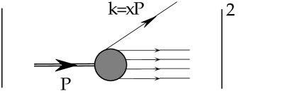
Figure 19: The classical parton model.

$f_{1}$ is expressed as a sum of probabilities to find a (light-cone quantized) quark with $p^{+}=xp$ and any transverse momentum, summed over helicities and weighted by the phase space factor $1/x$. Perhaps the reader is more familiar with the “infinite momentum frame” form of the model, where $f_{1}$ is written as the sum of probabilities to find an (equal-time quantized) quark with a fraction $x$ of the target’s (infinite) longitudinal momentum. The two formulations are equivalent since the boost to an infinite momentum frame is equivalent to a light-cone formulation. Since eq. (3.49) is valid in any frame, it can be used in (e.g.) the lab frame to provide parton distributions which can be associated with quark models.[18] One must, however, be careful to remember that the fields in eq. (3.49) are good light-cone Dirac components quantized at equal $\xi^{+}$, not equal $\xi^{0}$.

An identical calculation for $x<0$ captures antiquark operators and leads to the standard crossing relation for $f_{1}$,

$$f_{1}(x)=-\bar{f}_{1}(-x)$$ (3.50)

where $\bar{f}_{1}$ is given by eq. (3.49) with $R\rightarrow R_{c}$ and $L\rightarrow L_{c}$. The other (spin-dependent) quark distributions are explored in the following Section.

3.4.2 Twist-Three

Now let us apply the same analysis to the simplest twist-three distribution function,

$$\int{d\lambda\over 2\pi}e^{i\lambda x}\langle P|\bar{\psi}(0)\psi(\lambda n)|P\rangle\equiv 2Me(x).$$ (3.51)

Decomposing in terms of $\phi$ and $\chi$, we find

$$e(x)={1\over 2M}\int{d\lambda\over 2\pi}e^{i\lambda x}\langle P|\phi^{\dagger}(0)\gamma^{0}\chi(\lambda n)+\chi^{\dagger}(0)\gamma^{0}\phi(\lambda n)|P\rangle,$$ (3.52)

which contains the dynamically dependent operator $\chi$. If we use the constraint to eliminate $\chi$ we obtain

$$e(x)=-{1\over 4Mx}\int{d\lambda\over 2\pi}e^{i\lambda x}\langle P|\bar{\phi}(0)n/D/_{\perp}(\lambda n)\phi(\lambda n)|P\rangle+\mbox{h.c.}$$ (3.53)

So $e(x)$ is really a quark-gluon correlation function on the light-cone. It has no simple Fock-space interpretation in terms of quarks alone, despite the apparently simple form of eq. (3.51).

We have happened upon a general (and very useful) result: Every factor of $\chi$ in the light-cone decomposition of a light-cone correlation function contributes an additional unit of twist to the associated distribution function,

$$\phi^{\dagger}\phi \Leftrightarrow\mbox{Twist-2}$$

$$\phi^{\dagger}\chi \Leftrightarrow\mbox{Twist-3}$$

$$\chi^{\dagger}\chi \Leftrightarrow\mbox{Twist-4}.$$

Likewise each unit of twist introduces an additional independent field in the null plane correlator:

$$\mbox{Twist-2}\rightarrow\phi^{\dagger}(0)\phi(\lambda n)$$

$$\mbox{Twist-3}\rightarrow\phi^{\dagger}(0)D_{\perp}(\lambda n)\phi(\mu n)$$

$$\mbox{Twist-4}\rightarrow\phi^{\dagger}(0)D_{\perp}(\lambda n)D_{\perp}(\mu n)\phi(\nu n).$$

It is as if $\phi$ had twist-one and $\chi$ had twist-two.

Twist-three is tractable, using the methods that have been developed in these lectures. Twist-four requires a more extensive analysis based on operator product expansion methods developed during the 1980’s.[39, 19]. With these general tools in hand, we turn in the next section to the analysis of the specific distributions which appear in deep inelastic scattering of leptons.

4 Deep Inelastic Scattering and Generalized Distribution Functions II

In this section we use the tools developed in §3 to classify and interpret the quark distribution functions which appear in the analysis of DIS. The topics will include the classification and parton interpretation of the three leading twist quark distribution functions; a discussion of the physics of the less well known transversity distribution, $h_{1}$; a review of transverse spin in hard processes; a short digression on higher spin targets and gluon distribution functions; and a summary of the physics associated with the twist-three transverse spin distribution, $g_{2}$.

4.1 Helicity Amplitudes

Part of the task is simply to enumerate the independent distribution functions at twist-two and twist-three. This is simplified by viewing distribution functions as discontinuities in forward parton-(quark or gluon) hadron scattering. Suppressing all momentum indices, each quark distribution can be labeled by four helicities: a target of helicity $\Lambda$ emits a parton of helicity $\lambda$ which then participates in some hard scattering process. The resulting parton with helicity $\lambda^{\prime}$ is reabsorbed by a hadron of helicity $\Lambda^{\prime}$. The process of interest to us is actually a u-channel discontinuity of the forward parton-hadron scattering amplitude ${\cal A}_{\Lambda\lambda,\Lambda^{\prime}\lambda^{\prime}}$ as shown in fig. (20).

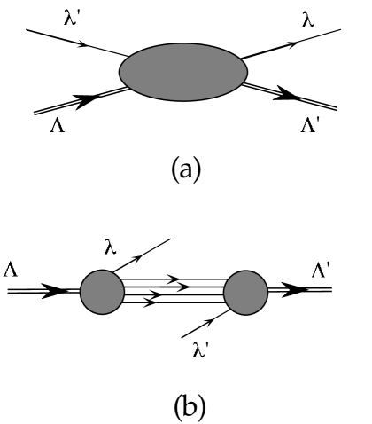
Figure 20: Helicity structure a) of the parton-hadron forward scattering amplitude; b) of the $u$-channel discontinuity which contributes to a parton distribution function.

Note the ordering of indices – although $\Lambda$ and $\lambda^{\prime}$ are the incoming helicities, it is convenient to label the amplitude in the sequence: initial hadron, struck quark, final hadron, returned quark.

Since the parton-hadron amplitude results from squaring something like $\left<X|\psi|PS\right>$, the amplitude must be diagonal in the target spin. However spin eigenstates (in particular, transverse spin eigenstates) are linear superpositions of helicity eigenstates, so the $\{{\cal A}\}$ do not have to be diagonal in the target helicity. Only forward scattering is of interest, so the initial and final helicities must be the same,

$$\Lambda+\lambda^{\prime}=\Lambda^{\prime}+\lambda.$$ (4.1)

Also, the parity and time reversal invariance of the strong interactions place constraints on the $\{{\cal A}\}$,

$${\cal A}_{\Lambda\lambda,\Lambda^{\prime}\lambda^{\prime}} = {\cal A}_{-\Lambda-\lambda,-\Lambda^{\prime}-\lambda^{\prime}}$$ (4.2)

$${\cal A}_{\Lambda\lambda,\Lambda^{\prime}\lambda^{\prime}} = {\cal A}_{\Lambda^{\prime}\lambda^{\prime},\Lambda\lambda}$$ (4.3)

respectively.

Clearly the helicity counting outlined above applies equally well to good and bad light-cone components of quark or gluon fields. Therefore we can use it together with the methods of the previous section to enumerate quark distribution function through twist-three. To work through twist-three we will have to consider the case of one good and one bad light-cone component. We will identify any bad light-cone fields in helicity amplitudes by an asterix on the helicity label. Thus ${\cal A}_{0{1\over 2},0{1\over 2}^{*}}$ corresponds to emission of a good light-cone component and absorption of a bad one.

4.2 Quark Distributions in Targets with Spin-0, 1/2 and 1

4.2.1 Spin-$0$ Target

Only $\Lambda=0$ is available. Parity equates ${\cal A}_{0{1\over 2},0{1\over 2}}$ and ${\cal A}_{0-{1\over 2},0-{1\over 2}}$. Time reversal equates ${\cal A}_{0{1\over 2},0{1\over 2}^{*}}$ and ${\cal A}_{0{1\over 2}^{*},0{1\over 2}}$. So there is only one distribution function at twist-two and one at twist-three. The twist-two function is none other than $f_{1}$ associated with the bilocal operator $\bar{\psi}(0)n/\psi(\lambda n)$ and conserves quark chirality (“chiral even”). The twist-three function is $e$, associated with the scalar bilocal operator $\bar{\psi}(0)\psi(\lambda n)$ and flips quark chirality (“chiral odd”). These properties are summarized by

Twist	$\Lambda$	$\lambda$		$\Lambda^{\prime}$	$\lambda^{\prime}$	Chirality
Two	$0$	$1/2\phantom{{}^{*}}$		$0$	$1/2$	Even
Three	$0$	${1/2}^{*}$		$0$	$1/2$	Odd

Table 1: Quark distributions in a spin-0 hadron through twist-three.

4.2.2 Spin-$1/2$ Target

In the spin-$1/2$ case, for each twist assignment there are three independent helicity amplitudes. The reader may wish to verify that parity and time reversal invariance relate the many helicity amplitudes to the six listed in the table below (through twist-three). We leave the interpretation of these six distribution functions for the next section where they are discussed in detail.

Twist	$\Lambda$	$\lambda$		$\Lambda^{\prime}$	$\lambda^{\prime}$	Chirality
Two	$\phantom{+}1/2$	$\phantom{+}1/2\phantom{{}^{*}}$		$\phantom{+}1/2$	$\phantom{+}1/2$	Even
Two	$\phantom{+}1/2$	$-1/2\phantom{{}^{*}}$		$\phantom{+}1/2$	$-1/2$	Even
Two	$\phantom{+}1/2$	$\phantom{+}1/2\phantom{{}^{*}}$		$-1/2$	$-1/2$	Odd
Three	$\phantom{+}1/2$	$\phantom{+}1/2^{*}$		$\phantom{+}1/2$	$\phantom{+}1/2$	Odd
Three	$\phantom{+}1/2$	$-1/2^{*}$		$\phantom{+}1/2$	$-1/2$	Odd
Three	$\phantom{+}1/2$	$\phantom{+}1/2^{*}$		$-1/2$	$-1/2$	Even

Table 2: Quark distributions in a spin-1/2 hadron through twist-three.

4.2.3 Spin-$1$ Target

A massive spin-one target has three independent helicity states. A new complication appears at twist-three: two helicity flip distributions arise which are not related by any of the symmetries of QCD. One can easily check that no such complication occurs for spin ${1\over 2}$. There is much interesting physics in these spin-one structure functions, however time will not permit us to work through it here. Instead we refer the interested reader to the original literature.[34, 35, 41, 42]

Twist	$\Lambda$	$\lambda$		$\Lambda^{\prime}$	$\lambda^{\prime}$	Chirality
Two	$1$	$\phantom{+}1/2\phantom{{}^{*}}$		$1$	$\phantom{+}1/2\phantom{{}^{*}}$	Even
Two	$1$	$-1/2\phantom{{}^{*}}$		$1$	$-1/2\phantom{{}^{*}}$	Even
Two	$0$	$\phantom{+}1/2\phantom{{}^{*}}$		$0$	$\phantom{+}1/2\phantom{{}^{*}}$	Even
Two	$0$	$-1/2\phantom{{}^{*}}$		$1$	$\phantom{+}1/2\phantom{{}^{*}}$	Odd
Three	$1$	$\phantom{+}1/2^{*}$		$1$	$\phantom{+}1/2\phantom{{}^{*}}$	Even
Three	$1$	$-1/2^{*}$		$1$	$-1/2\phantom{{}^{*}}$	Even
Three	$0$	$\phantom{+}1/2^{*}$		$0$	$\phantom{+}1/2\phantom{{}^{*}}$	Even
Three	$0$	$-1/2^{*}$		$1$	$\phantom{+}1/2\phantom{{}^{*}}$	Odd
Three	$0$	$-1/2\phantom{{}^{*}}$		$1$	$\phantom{+}1/2^{*}$	Odd

Table 3: Quark distributions in a spin-1 hadron through twist-three.

4.3 Quark Distribution Functions for the Nucleon

The distribution functions for a spin-${1\over 2}$ target deserve special attention because protons and neutrons are the principal targets of interest. In Table 4 the quark distribution functions for a nucleon target are listed through twist-three. They are classified according to their twist (or light-cone projection) and their helicity.

twist $O(1/Q^{t-2})$	Name	Helicity Amplitude	Measurement	Chirality
Two	$f_{1}$	${\cal A}_{1{1\over 2},1{1\over 2}}+{\cal A}_{1-{1\over 2},1-{1\over 2}}$	Spin average	Even
Two	$g_{1}$	${\cal A}_{1{1\over 2},1{1\over 2}}-{\cal A}_{1-{1\over 2},1-{1\over 2}}$	Helicity difference	Even
Two	$h_{1}$	${\cal A}_{0{1\over 2},1-{1\over 2}}$	Helicity flip	Odd
Three	$e$	${\cal A}_{1{1\over 2}^{*},1{1\over 2}}+{\cal A}_{1-{1\over 2},1-{1\over 2}}$	Spin average	Odd
Three	$h_{L}$	${\cal A}_{1{1\over 2}^{*},1{1\over 2}}-{\cal A}_{1-{1\over 2},1-{1\over 2}}$	Helicity difference	Odd
Three	$g_{T}$	${\cal A}_{0{1\over 2}^{*},1-{1\over 2}}$	Helicity flip	Even

Table 4: Nucleon structure functions classified according to their twist and target helicities.

The distribution functions $f_{1}$, $g_{1}$ and $g_{T}$ are familiar because they can be measured in lepton scattering. The others are less well known, but are essential to understand the nucleon spin substructure in deep inelastic processes. All of them are defined by the matrix elements of quark bilocal operators,

$$\int{d\lambda\over{2\pi}}e^{i\lambda x}\left<PS|\bar{\psi}(0)\gamma_{\mu}\psi(\lambda n)|PS\right> = 2\left\{f_{1}(x)p_{\mu}+M^{2}f_{4}(x)n_{\mu}\right\},$$

$$\int{d\lambda\over{2\pi}}e^{i\lambda x}\left<PS|\bar{\psi}(0)\gamma_{\mu}\gamma_{5}\psi(\lambda n)|PS\right> = 2\left\{g_{1}(x)p_{\mu}S\cdot n+g_{T}(x)S_{\perp\mu}+M^{2}g_{3}(x)n_{\mu}S\cdot n\right\},$$

$$\int{d\lambda\over{2\pi}}e^{i\lambda x}\left<PS|\bar{\psi}(0)\psi(\lambda n)|PS\right> = 2e(x),$$

$$\int{d\lambda\over{2\pi}}e^{i\lambda x}\left<PS|\bar{\psi}(0)i\sigma_{\mu\nu}\gamma_{5}\psi(\lambda n)|PS\right> = 2\{h_{1}(x)(S_{\perp\mu}p_{\nu}-S_{\perp\nu}p_{\mu})/M$$ (4.4)

$$+ h_{L}(x)M(p_{\mu}n_{\nu}-p_{\nu}n_{\mu})S\cdot n$$

$$+ h_{3}(x)M(S_{\perp\mu}n_{\nu}-S_{\perp\nu}n_{\mu})\},$$

Some twist-four distributions ($f_{4}$, $g_{3}$, and $h_{3}$) appear in these matrix elements. However, they are joined by many other quark-quark and quark-gluon distributions from which they cannot be separated, so there is no point in keeping track of them in this analysis.

4.3.1 Nucleon Spin Structure at Twist-Two

$f_{1}$, $g_{1}$ and $h_{1}$ are twist-two, i.e. they scale modulo logarithms. They can be projected out of the general decompositions, eq. (4.4),

$$f_{1}(x) = \int{d\lambda\over{4\pi}}e^{i\lambda x}\langle P|\bar{\psi}(0)n/\psi(\lambda n)|P\rangle$$

$$g_{1}(x) = \int{d\lambda\over{4\pi}}e^{i\lambda x}\langle PS_{\parallel}|\bar{\psi}(0)n/\gamma_{5}\psi(\lambda n)|PS_{\parallel}\rangle$$

$$h_{1}(x) = \int{d\lambda\over{4\pi}}e^{i\lambda x}\langle PS_{\perp}|\bar{\psi}(0)[S/_{\perp},n/]\gamma_{5}\psi(\lambda n)|PS_{\perp}\rangle$$ (4.5)

To understand their physical significance — in particular, to see why a third quark distribution in addition to $f_{1}$ and $g_{1}$ is necessary to describe the nucleon’s quark spin substructure at leading twist in the parton model — it suffices to decompose them with respect to a light-cone Fock space basis. If we use the helicity basis, then

$$f_{1}(x) = \frac{1}{x}\left<P|R^{\dagger}(xp)R(xp)+L^{\dagger}(xp)L(xp)|P\right>,$$

$$g_{1}(x) = \frac{1}{x}\left<P\hat{e}_{3}|R^{\dagger}(xp)R(xp)-L^{\dagger}(xp)L(xp)|P\hat{e}_{3}\right>,$$

$$h_{1}(x) = \frac{2}{x}Re\left<P\hat{e}_{1}|L^{\dagger}(xp)R(xp)|P\hat{e}_{1}\right>,$$ (4.6)

in analogy with eq. (3.49), where we have integrated out the dependence on transverse momentum. Here $\hat{e}_{3}$ and $\hat{e}_{1}$ are unit vectors parallel and transverse, respectively, to the target nucleon’s three-momentum. Clearly $f_{1}$ and $g_{1}$ can be interpreted in a probabilistic way: $f_{1}$ measures quarks independent of their helicity and $g_{1}$ measures the helicity asymmetry. But $h_{1}$ does not appear to have a probabilistic interpretation, instead it mixes right and left handed quarks.

If instead we use a transversity basis, diagonalizing $\gamma^{1}$, we find,

$$f_{1}(x) = \frac{1}{x}\langle P|\alpha^{\dagger}(xp)\alpha(xp)+\beta^{\dagger}(xp)\beta(xp)|P\rangle,$$

$$g_{1}(x) = \frac{2}{x}{\rm Re}\langle P\hat{e}_{3}|\alpha^{\dagger}(xp)\beta(xp)|P\hat{e}_{3}\rangle,$$

$$h_{1}(x) = \frac{1}{x}\langle P\hat{e}_{1}|\alpha^{\dagger}(xp)\alpha(xp)-\beta^{\dagger}(xp)\beta(xp)|P\hat{e}_{1}\rangle.$$ (4.7)

Clearly $h_{1}$ can be interpreted as the probability to find a quark with spin polarized along the transverse spin of a polarized nucleon minus the probability to find it polarized oppositely. $f_{1}$ still has the same interpretation, while now $g_{1}$ lacks a clear probabilistic interpretation. Of course the structure here is merely that of a $2\otimes 2$ – spin density matrix, with the assignments $f_{1}\leftrightarrow 1$, $g_{1}\leftrightarrow\sigma_{3}$, and $h_{1}\leftrightarrow\sigma_{1}$ in the basis of helicity eigenstates. The remaining element, $\sigma_{2}$, is related to $h_{1}$ by rotation about the $\hat{e}_{3}$-axis. In non-relativistic situations, spin and space operations (Euclidean boosts, etc.) commute and it is easy to show that $g_{1}=h_{1}$, so $h_{1}$ is a measure of the relativistic nature of the quarks inside the nucleon.

The chirally odd structure functions like $h_{1}$ fig. (fig. 21a) are suppressed in DIS. The dominant handbag diagram fig. (fig. 21b) as well as the various decorations which generate $\log Q^{2}$ dependences, $\alpha_{QCD}(Q^{2})$ corrections and higher twist corrections, examples of which are shown in figs. 21c-e involve only chirally-even quark distributions because the quark couplings to the photon and gluon preserve chirality. Only the quark mass insertion, fig. (21f), flips chirality. So up to corrections of order $m_{q}/Q$, $h_{1}(x,Q^{2})$ decouples from electron scattering.

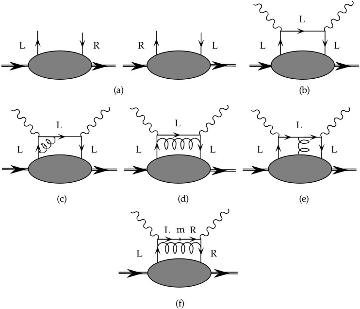
Figure 21: Chirality in deep inelastic scattering: a) Chirally odd contributions to $h_{1}(x)$; b)-e) Chirally even contributions to deep inelastic scattering (plus $L\leftrightarrow R$ for electromagnetic currents); f) Chirality flip by mass insertion.

There is no analogous suppression of $h_{1}(x,Q^{2})$ in deep inelastic processes with hadronic initial states such as Drell-Yan. The argument can be read from the standard parton diagram for Drell-Yan, fig. (22). Although chirality is conserved on each quark line separately, the two quarks’ chiralities are unrelated. It is not surprising, then, that Ralston and Soper [43] found that $h_{1}(x,Q^{2})$ determines the transverse-target, transverse-beam asymmetry in Drell-Yan.

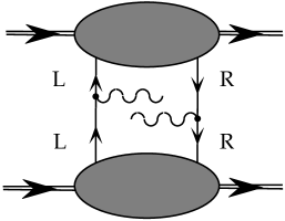
Figure 22: Chirality in Drell-Yan (plus $L\leftrightarrow R$) production of lepton pairs .

4.4 Transverse Spin in QCD

The simple structure of eqs. (4.6) and (4.7 ) shows that transverse spin effects and longitudinal spin effects are on a completely equivalent footing in perturbative QCD. On the other hand, $h_{1}$ was unknown in the early days of QCD when only deep inelastic lepton scattering was studied in detail.

Not knowing about $h_{1}$, many authors, beginning with Feynman[44], have attempted to interpret $g_{T}$ as the natural transverse spin distribution function. Since $g_{T}$ is twist-three and interaction dependent, this attempt led to the erroneous impression that transverse spin effects were inextricably associated with off-shellness, transverse momentum and/or quark-gluon interactions The resolution contained in the present analysis is summarized in Table 5 where the symmetry between transverse and longitudinal spin effects is apparent. Only ignorance of $h_{1}$ and $h_{L}$ prevented the appreciation of this symmetry at a much earlier date.

	Longitudinal	Transverse
	Spin	Spin
Twist-2	$g_{1}(x,Q^{2})$	$h_{1}(x,Q^{2})$
Twist-3	$h_{L}(x,Q^{2})$	$g_{T}(x,Q^{2})$

Table 5: The transverse and longitudinal spin distribution functions through twist-three.

Since experiments to measure $h_{1}$ are being planned, now is the time for theorists to make predictions. At this time, however, not much is known about either the general behavior of $h_{1}$ or its form in models. Here is a summary, presented in parallel with $g_{1}$ for the purpose of comparison.

• Inequalities:

  $$|g_{1}(x,Q^{2})| \leq f_{1}(x,Q^{2})$$

  $$|h_{1}(x,Q^{2})| \leq f_{1}(x,Q^{2})$$ (4.8)

  for each flavor of quark and antiquark. These follow from the positivity of parton probability distributions (see eqs. (4.6) and (4.7)). Another inequality, proposed by Soffer[46] has attracted attention recently,

  $$f_{1}^{a}(x,Q^{2})+g_{1}^{a}(x,Q^{2})\geq 2|h_{1}^{a}(x,Q^{2})|.$$ (4.9)

  valid for each flavor ($a$) of quark and antiquark. Soffer’s inequality is invalidated by QCD radiative corrections,[12] in much the same way as the Callan-Gross relation, $F_{2}=2xF_{2}$. Despite this problem, the inequality may prove to be a useful qualitative guide to the magnitude of $h_{1}$. A recent discussion of QCD radiative corrections to Soffer’s inequality may be found in [47].

• Physical interpretation: The structure function $h_{1}(x,Q^{2})$ measures transversity. It is chirally odd and related to a bilocal generalization of the tensor operator, $\bar{q}\sigma_{\mu\nu}i\gamma_{5}q$. On the other hand $g_{1}(x,Q^{2})$ measures helicity. It is chirally even and related to a bilocal generalization of the axial charge operator, $\bar{q}\gamma_{\mu}\gamma_{5}q$. Although $h_{1}$ is spin-dependent, it is not directly related to the quark or nucleon spin. It would be very useful to have a better idea of the dynamical and relativistic effects which generate differences between $g_{1}$ and $h_{1}$.

• Sum rules: If we define a “tensor charge” in analogy to the axial vector charge measured in $\beta$–decay,

  $$2S^{i}\delta q^{a}(Q^{2})\equiv\langle PS|\bar{q}\sigma^{0i}i\gamma_{5}{\lambda^{a}\over 2}q\Big{|}_{Q^{2}}|PS\rangle,$$ (4.10)

  where $\lambda^{a}$ is a flavor matrix and $Q^{2}$ is a renormalization scale, then $\delta q^{a}(Q^{2})$ is related to an integral over $h_{1}^{a}(x,Q^{2})$,

  $$\delta q^{a}(Q^{2})=\int_{0}^{1}dx(h_{1}^{a}(x,Q^{2})-h_{1}^{\bar{a}}(x,Q^{2}))$$ (4.11)

  where $h_{1}^{a}$ and $h_{1}^{\bar{a}}$ receive contributions from quarks and antiquarks, respectively. The analogous expressions for $g_{1}(x,Q^{2})$ involve axial charges,

  $$2s^{i}\Delta q^{a}(Q^{2}) \equiv \langle PS|\bar{q}\gamma^{i}\gamma_{5}{\lambda^{a}\over 2}q\Big{|}_{Q^{2}}|PS\rangle$$ (4.12)

  $$\Delta q^{a}(Q^{2}) = \int_{0}^{1}dx(g_{1}^{a}(x,Q^{2})+g_{1}^{\bar{a}}(x,Q^{2})).$$ (4.13)

  Note the contrast: $h_{1}(x,Q^{2})$ is not normalized to a piece of the angular momentum tensor, so $h_{1}$, unlike $g_{1}$, cannot be interpreted as the fraction of the nucleons’ spin found on the quarks’ spin. Note the sign of the antiquark contributions: $\delta q^{a}$ is charge-conjugation odd, whereas $\Delta q^{a}$ is charge-conjugation even. $\delta q^{a}$ gets no contribution from quark-antiquark pairs in the sea. All tensor charges $\delta q^{a}$ have non-vanishing anomalous dimensions [48], but none mix with gluonic operators under renormalization because they are chirally odd and gluon operators are even. In contrast, the flavor non-singlet axial charges, $\Delta q^{a},a\neq 0$, have vanishing anomalous dimensions, whereas the singlet axial charge $\Delta q^{0}$ has an anomalous dimension arising from the triangle anomaly.[49]

• Evolution: It is worth re-emphasizing that $h_{1}$ has unusual QCD evolution properties. All of the local operators associated with $h_{1}$ have non-vanishing leading order anomalous dimensions. On the other hand, no gluon operators contribute to $h_{1}$ in any order, because $h_{1}$ is chiral odd. So $h_{1}$ is a non-singlet structure function – it evolves homogeneously with $Q^{2}$, but none of its moments are $Q^{2}$ independent.

• Models: $h_{1}$ and $g_{1}$ are identical in non-relativistic quark models, but differ in relativistic models like the bag model - see fig. (23).

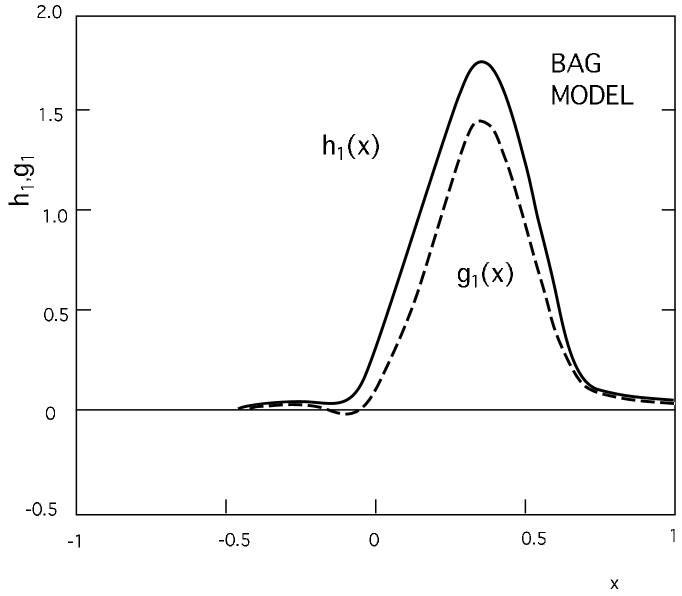
Figure 23: Bag model calculation for $h_{1}$ and $g_{1}$ from [8, 9].

4.5 Twist-Three: Physics with $g_{2}(x,Q^{2})$

There are several reasons to be particularly interested in the transverse spin dependent structure function, $g_{2}(x,Q^{2})$

1. it can be measured in deep inelastic scattering;

2. it is unique among higher twist distributions in that it dominates the cross section in a specific kinematic domain — at $90^{\circ}$ all twist-two effects decouple, see eq. (LABEL:eq:spindepxsection);

3. it is related to interesting quark gluon matrix elements;

4. it should obey an interesting sum rules.

For a review of the properties of $g_{2}$, see ref. [15]

4.5.1 Operator Product Expansion

The spin structure functions $g_{1}$ and $g_{2}$ parameterize the antisymmetric part of the hadronic tensor $W_{\mu\nu}$ as shown in eq. (1.15). Applying the methods of §2 we can relate the moments of the antisymmetric part of $W_{\mu\nu}$ to the matrix elements of quark operators accurate through twist-three. Consider the antisymmetric part of the forward Compton amplitude $T_{\mu\nu}$:

$$T_{[\mu\nu]} = \frac{1}{2}\left[T_{\mu\nu}-T_{\nu\mu}\right],$$

$$= \left<PS|{\cal T}_{[\mu\nu]}(q)|PS\right>,\quad{\rm where}$$

$${\cal T}_{[\mu\nu]}(q) = \int d^{4}\xi e^{iq\cdot\xi}T(J_{[\mu}(\xi)J_{\nu]}(0)).$$ (4.14)

The leading twist (twists-two and -three) contributions come from the series of operators

$${\cal T}_{[\mu\nu]}=i\epsilon_{\mu\nu\lambda\sigma}q^{\lambda}\sum\limits_{n=0,2,4\dots}q^{\mu_{1}}\dots q^{\mu_{n}}\Theta^{\sigma}_{\{\mu_{1}\dots\mu_{n}\}}\left(\frac{-2}{q^{2}}\right)^{n+1}C_{n}(q^{2}).$$ (4.15)

with

$$\Theta_{\sigma\{\mu_{1}\dots\mu_{n}\}}\equiv i^{n}\bar{\psi}\gamma_{\sigma}\gamma_{5}D_{\{\mu_{1}}\dots D_{\mu_{n}\}}\psi-{\rm traces},$$ (4.16)

Here $\{\hskip 5.69054pt,\hskip 5.69054pt\}$ denotes symmetrization and $[\hskip 5.69054pt,\hskip 5.69054pt]$ denotes antisymmetrization of the enclosed indices. The string of symmetric indices originates in the expansion of the bilocal operator about $\xi=0$, and contraction of each index with $q^{\mu}$ selects the totally symmetric part. On the other hand, the index on the $\gamma$–matrix is not symmetrized. $C_{n}(q^{2})$ is the coefficient function and is unity to lowest order. Flavor factors such as squared charges are suppressed.

Eq. (4.16) can be split into a totally symmetric part and a part of lower symmetry,

$$\Theta_{\sigma\{\mu_{1}\dots\mu_{n}\}}\equiv\Theta_{\{\sigma\mu_{1}\dots\mu_{n}\}}+\Theta_{[\sigma\{\mu_{1}]\mu_{2}\dots\mu_{n}\}},$$ (4.17)

where the first term has twist-two (dimension $n+3$, spin $n+1$):

$$\Theta_{\{\sigma\mu_{1}\dots\mu_{n}\}}=\frac{1}{n+1}\left\{\Theta_{\sigma\{\mu_{1}\dots\mu_{n}\}}+\Theta_{\mu_{1}\{\sigma\mu_{2}\dots\mu_{n}\}}+\Theta_{\mu_{2}\{\mu_{1}\sigma\dots\mu_{n}\}}+\dots\right\},$$ (4.18)

and the second term, with no totally symmetric part, has twist-three (dimension $n+3$, spin $n$):

$$\Theta_{[\sigma\{\mu_{1}]\mu_{2}\dots\mu_{n}\}} = \frac{1}{n+1}\Big{\{}\Theta_{\sigma\{\mu_{1}\dots\mu_{n}\}}-\Theta_{\mu_{1}\{\sigma\mu_{2}\dots\mu_{n}\}}$$ (4.19)

$$+ \Theta_{\sigma\{\mu_{1}\dots\mu_{n}\}}-\Theta_{\mu_{2}\{\mu_{1}\sigma\dots\mu_{n}\}}+\dots\Big{\}}.$$

The proton matrix elements of these operators are

$$\left<PS|\Theta_{\{\sigma\mu_{1}\dots\mu_{n}\}}|PS\right> = \left\{S_{\sigma}P_{\mu_{1}}\dots P_{\mu_{n}}+S_{\mu_{1}}P_{\sigma}\dots P_{\mu_{n}}+\dots\right\}\frac{a_{n}}{n+1},$$

$$\left<PS|\Theta_{[\sigma\{\mu_{1}]\mu_{2}\dots\mu_{n}\}}|PS\right> = \left\{(S_{\sigma}P_{\mu_{1}}-S_{\mu_{1}}P_{\sigma})P_{\mu_{2}}\dots P_{\mu_{n}}\right.$$ (4.20)

$$+ \left.(S_{\sigma}P_{\mu_{2}}-S_{\mu_{2}}P_{\sigma})P_{\mu_{1}}\dots P_{\mu_{n}}+\dots\right\}\frac{d_{n}}{n+1}.$$

4.5.2 Wandzura – Wilczek Decomposition of $g_{2}$

Extracting the relation between these matrix elements and the moments of $g_{1}$ and $g_{2}$ is an exercise in the methods of §2. Substituting these matrix elements into the definition of $T_{[\mu\nu]}$, writing a dispersion relation in terms of $g_{1}$ and $g_{2}$ and equating terms in the Taylor expansion in $1/x$ in the BJL–limit, we find

$$\int\limits_{0}^{1}dxx^{n}g_{1}(x,Q^{2}) = \frac{1}{4}a_{n}\quad n=0,2,4,\dots,$$

$$\int\limits_{0}^{1}dxx^{n}g_{2}(x,Q^{2}) = \frac{1}{4}\frac{n}{n+1}\left(d_{n}-a_{n})\right),\quad n=2,4\dots,$$ (4.21)

Notice that the same operators which determine $g_{1}$ make an appearance in the moments of $g_{2}$. It follows that $g_{2}$ can be decomposed into two parts, one which is fixed by $g_{1}$, and another — the “true twist-three” part — associated with the operator of mixed symmetry,

$$g_{2}(xQ^{2})=-g_{1}(x,Q^{2})+\int\limits_{x}^{1}\frac{dy}{y}g_{1}(y,Q^{2})+\bar{g}_{2}(x,Q^{2}).$$ (4.22)

Wandzura and Wilczek proposed this decomposition in 1977.[50] They went further and suggested that $\bar{g}_{2}$ might be zero. From another perspective, $\bar{g}_{2}$ is the interesting part of $g_{2}$. It’s moments,

$$\int\limits_{0}^{1}dxx^{n}\bar{g}_{2}(x,Q^{2})=\frac{n}{4(n+1)}d_{n}(Q^{2}),$$ (4.23)

are twist-three and measure quark-gluon correlations, as was pointed out by Shuryak and Vainshteyn[51]. They showed that the $QCD$ equations of motion can be used to trade the antisymmetry of $\Theta_{[\sigma\{\mu_{1}]\mu_{2}\dots\mu_{n}\}}$ for factors of the gluon field strength $G_{\mu\nu}$ and the QCD coupling constant $g$. The result is:

$$\Theta_{[\sigma\{\mu_{1}]\mu_{2}\dots\mu_{n}\}} = \frac{g}{8}{\cal S}_{n}\left\{\sum\limits_{l=0}^{n-2}i^{n-2}\bar{\psi}D_{\mu_{1}}..D_{\mu_{l}}\tilde{G}_{\sigma\mu_{l+1}}D_{\mu_{l+2}}..D_{\mu_{n-1}}\gamma_{\mu_{n}}\psi\right.$$ (4.24)

$$+ \left.\frac{1}{2}\sum\limits_{l=0}^{n-3}i^{n-3}\bar{\psi}D_{\mu_{1}}..D_{\mu_{l}}(D_{\mu_{l+1}}G_{\sigma\mu_{l+2}})D_{\mu_{l+3}}..D_{\mu_{n-1}}\gamma_{\mu_{n}}\gamma_{5}\psi\right\},$$

where $\tilde{G}_{\alpha\beta}=\frac{1}{2}\epsilon_{\alpha\beta\lambda\sigma}G^{\lambda\sigma}$ and ${\cal S}_{n}$ symmetrizes the indices $\mu_{1}\dots\mu_{n}$.

Eq. (4.24) is quite formidable. A simpler example might help explain how manipulation of the equations of motion exposes the interaction dependence of higher twist operators. Consider the twist-three operator,

$$X_{\mu\nu}=\bar{\psi}D_{\mu}D_{\nu}\psi$$ (4.25)

as an example. $X$ is clearly twist-three (dimension five, spin no greater than two). One might be tempted to make a “parton model” for the matrix element of $X$, by replacing $D_{\mu}\rightarrow\partial_{\mu}$ and evaluating $X$ in a beam of collinear quarks. That, however, would be a mistake, since application of the identity $D_{\mu}=\frac{1}{2}\{\gamma_{\mu},D/\}$, and the QCD equations of motion, $D/\psi=\bar{\psi}D/=0$ and $[D_{\mu},D_{\nu}]=gG_{\mu\nu}$, yields

$$X_{\mu\nu}=\frac{g}{2}\bar{\psi}G_{\mu\lambda}\gamma^{\lambda}\gamma_{\nu}\psi.$$ (4.26)

So it is clear that $X$ and its matrix elements are interaction dependent and measure a quark-gluon correlation in the target hadron. This is a special case of a general result that operators of twist $\geq 3$ can always be written in a form in which they are manifestly interaction dependent. In particular one has:

$$\int_{0}^{1}x^{2}\bar{g}_{2}(x,Q^{2})\propto\langle PS|{1\over 8}g{\cal S}_{\mu_{1}\mu_{2}}\bar{\psi}\tilde{G}_{\sigma\mu_{1}}\gamma_{\mu_{2}}\psi|PS\rangle.$$ (4.27)

Model builders or lattice enthusiasts who want to predict $g_{2}$ must confront such matrix elements.

4.5.3 The Burkhardt Cottingham Sum Rule

A striking consequence of the light-cone analysis of $g_{2}$ is the apparent sum rule,[52]

$$\int\limits_{0}^{1}dxg_{2}(x,Q^{2})=0,$$ (4.28)

which follows directly from eq. (4.21) with $n=0$. If true, the sum rule requires $g_{2}$ to have a node (other than at $0$ and $1$).

The Burkhardt-Cottingham (BC) Sum Rule looks to be a consequence of rotation invariance. To see this, return to eq. (4.4) and consider the $\gamma_{\mu}\gamma_{5}$ case in the laboratory frame (where $S^{0}=0$). First, set $\hat{S}=M\hat{e}_{3}$, contract the free Lorentz index with $n^{\mu}$ and integrate overall $x$, leaving

$$\int\limits_{-1}^{1}dxg_{1}(x,Q^{2})=\langle P\hat{e}_{3}|\bar{q}(0)\gamma^{3}\gamma_{5}q(0)|_{Q^{2}}|P\hat{e}_{3}\rangle.$$ (4.29)

Next repeat the process with $\hat{S}=M\hat{e}_{1}$ and $\mu=1$, with the result,

$$\int\limits_{-1}^{1}dxg_{T}(x,Q^{2})=\langle P\hat{e}_{1}|\bar{q}(0)\gamma^{1}\gamma_{5}q(0)|_{Q^{2}}|P\hat{e}_{1}\rangle.$$ (4.30)

The right hand sides of these two equations are equal in the rest frame by rotation invariance, so

$$\int_{-1}^{1}dxg_{T}(x,Q^{2})=\int_{-1}^{1}dxg_{1}(x,Q^{2}),$$ (4.31)

whence

$$\int_{-1}^{1}dxg_{2}(x,Q^{2})=0,$$ (4.32)

apparently a consequence of rotation invariance.

The subtlety in this derivation is that the integral in eq. (4.32) goes from $-1$ to $1$ including $x=0$. As we have defined it, $g_{2}(x,Q^{2})$ is the limit of a function of $Q^{2}$ and $\nu$ and therefore might contain a distribution ($\delta$–functions, etc.) at $x=0$. Suppose $g_{2}$ has a $\delta$–function contribution at $x=0$,

$$g_{2}(x,Q^{2})=g_{2}^{\rm observable}(x,Q^{2})+c\delta(x).$$ (4.33)

Then since experimenters cannot reach $x=0$, the BC sum rule reads

$$\int_{0}^{1}dxg_{2}^{\rm observable}(x,Q^{2})=-{1\over 2}c,$$ (4.34)

which is useless.

This pathology — a $\delta$–function at $x=0$ — is not as arbitrary as it looks. Instead it is an example of a disease known as a “$J=0$ fixed pole with non-polynomial residue”. First studied in Regge theory,[53, 27] a $\delta(x)$ in $g_{2}(x,Q^{2})$ corresponds to a real constant term in a spin flip Compton amplitude which persists to high energy. There is no fundamental reason to exclude such a constant. On the other hand the sum rule is known to be satisfied in QCD perturbation theory through order $O(g^{2})$. The sum rule has been studied recently by several groups who find no evidence for a $\delta(x)$ in perturbative QCD.[54, 55, 56] So at least provisionally, we must regard this as a reliable sum rule. At least one other sum rule of interest experimentally, the Gerasimov, Drell, Hearn Sum Rule for spin dependent Compton scattering has the same potential pathology. For further discussion of the BC sum rule see ref. [15].

4.5.4 The Evolution of $g_{2}$

The following discussion can be regarded as a “theoretical interlude” and may be omitted by the casual reader.

The $Q^{2}$ evolution of quark distribution functions is an unavoidable complication in perturbative QCD. Data are inevitably taken at different $Q^{2}$, making it difficult to evaluate sum rules (which require data at some definite $Q^{2}$) without some information about $Q^{2}$–evolution. At leading twist the subject is well understood and we have ignored it. The evolution of $g_{2}$ is more complicated. Eq. (4.4) provides as deceptively simple operator representation of $g_{T}$,

$$g_{T}(x,q^{2}) = g_{1}(x,q^{2})+g_{2}(x,q^{2})$$ (4.35)

$$= \int{d\lambda\over 4\pi}e^{i\lambda x}\langle PS_{\perp}|\bar{\psi}(0)S/_{\perp}\gamma_{5}\psi(\lambda n)|_{Q^{2}}|PS_{\perp}\rangle$$

It looks as though $g_{T}$ is determined by a single operator which evolves homogeneously. However, the operator in eq. (4.35) is equivalent to the series of quark gluon operators given in eq. (4.24). Worse still, all these operators mix under renormalization. The number of operators that mix grows linearly with $n$. Back in the 1970’s, Ahmed and Ross calculated the anomalous dimension matrix element for the evolution of the transverse quark axial current operator in eq. (4.35).[57] In 1982 Shuryak and Vainshteyn pointed out that this was but one element of an $n\times n$ anomalous dimension matrix[51]. Later Ratcliffe, Lipatov et al. and others calculated the full anomalous dimension matrix.[58, 59, 60, 61]

Underlying this matrix renormalization group evolution is a somewhat simpler parton picture. The fundamental objects for studying the evolution of $g_{2}$ are two-variable parton distribution functions defined by double light-cone fourier transforms[7].

$$\int{d\lambda\over 2\pi}{d\mu\over 2\pi}e^{i\lambda x+i\mu(y-x)}\langle PS|\bar{q}(0)iD^{\alpha}(\mu n)n/q(\lambda n)|_{Q^{2}}|PS\rangle = 2i\varepsilon^{\alpha\beta\sigma\tau}n_{\beta}S_{\sigma}p_{\tau}G(x,y,Q^{2})$$

$$+ \ldots$$

$$\int{d\lambda\over 2\pi}{d\mu\over 2\pi}e^{i\lambda x+i\mu(y-x)}\langle PS|\bar{q}(0)iD^{\alpha}(\mu n)n/\gamma_{5}q(\lambda n)|_{Q^{2}}|PS\rangle = 2i\varepsilon^{\alpha\beta\sigma\tau}n_{\beta}S_{\sigma}p_{\tau}\tilde{G}(x,y,Q^{2})$$

$$+ \ldots$$

where $\ldots$ denote other tensor structures of twist greater than three. The functions $G(x,y,Q^{2})$ and $\tilde{G}(x,y,Q^{2})$ are generalizations of parton distributions describing the amplitude to find quarks and gluons with momentum fractions $x$, $y$ and $x-y$ in the target nucleon. They can be represented diagrammatically as in fig. (24).

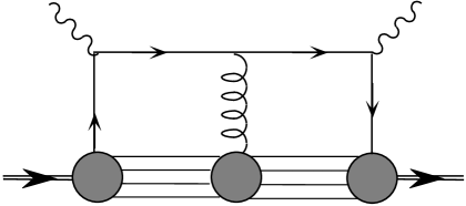
Figure 24: Quark/gluon diagram contributing to the two-variable parton distribution functions $G$ and $\tilde{G}$.

These “higher twist distribution functions” share many properties with leading twist. Only good light-cone components and collinear momenta appear – transverse momentum has been eliminated in favor of the interactions which generate it. The variables $x$, $y$, and $x-y$ take on only physical values, $-1\leq(x,y,x-y)\leq 1$, corresponding to emission or absorption of quarks, antiquarks or gluons.[40]

At any value of $Q^{2}$, $g_{T}(x,Q^{2})$ can be projected out by integrating out the variable $y$,

$$g_{T}(x,Q^{2})={1\over 2x}\int_{-1}^{1}dy\{G(x,y,Q^{2})-G(y,x,Q^{2})+\tilde{G}(x,y,Q^{2})-\tilde{G}(y,x,Q^{2})\}$$ (4.37)

The reason for introducing $G$ and $\tilde{G}$ is that they obey natural generalizations of the Gribov-Lipatov-Altarelli-Parisi (GLAP) evolution equations. Schematically,

$${d\over d\,\mbox{ln}\,Q^{2}}G(x,y,Q^{2})={\alpha_{QCD}\over 2\pi}\int_{x}^{1}\int_{y}^{1}dx^{\prime}dy^{\prime}{\cal P}(x,x^{\prime},y,y^{\prime})G(x^{\prime},y^{\prime},Q^{2})$$ (4.38)

for some “splitting function”, ${\cal P}$. In order to evolve $g_{T}$ from one $Q^{2}$ to another it is necessary to know $G$ and $\tilde{G}$ as a function of both $x$ and $y$. However, measurement of $g_{T}$ does not supply that information. $g_{T}$ is, in a sense, a “compressed” structure function. Information essential to evolution has been integrated out of it. The associated “open” distributions, $G$ and $\tilde{G}$ evolve simply. $g_{T}$ does not.

The situation is not entirely hopeless, however. It appears that the evolution of $g_{2}$ may simplify in the $N_{c}\rightarrow\infty$ limit, especially at large $x$.[62] Ali, Braun and Hiller showed that in this limit $\bar{g}_{2}$ obeys a standard GLAP equation, albeit with non-standard anomalous dimensions. As measurements of $g_{2}$ improve, theorists will be forced to expend more effort to clarify the nature of $Q^{2}$ evolution of $g_{T}$.

4.5.5 The Shape of $g_{2}$

With the first measurements of $g_{2}$ now available,[63] and more accurate measurements expected soon, it seems timely to review model predictions. First, here is an agenda of progressively more detailed questions for experimenters as they relate to theory

• Is $g_{2}$ zero?

  The answer is in on this one: the new SLAC data show $g_{2}\neq 0$.

• Is $\int_{0}^{1}dxg_{2}(x,Q^{2})$ zero as required by the BC sum rule?

  The SLAC data are consistent with the BC sum rule, albeit with large errors.

• If $\int_{0}^{1}dxg_{2}(x,Q^{2})=0$, then $g_{2}$ must have at least one non-trivial zero (besides $x=1$ and perhaps $x=0$). Is there just one such node?

  The SLAC data are consistent with one node, again within large errors.

• If there is only one non-trivial node, what is the sign of

  $$M_{2}[g_{2}]\equiv\int_{0}^{1}dxg_{2}(x,Q^{2})?$$ (4.39)

  With only one non-trivial node, the sign of $M_{2}$ determines the gross structure of $g_{2}$. If $M_{2}$ is positive $g_{2}$ is negative at small $x$ and positive at large $x$, and vica versa if $M_{2}$ is negative. The Wandzura-Wilczek (WW) contribution to $g_{2}$ gives $M_{2}^{WW}<0$.

  The SLAC data favor $M_{2}<0$.

• Is there a signal for $\bar{g}_{2}$ or does the WW contribution account for all of $g_{2}$?

  The SLAC data agree rather well with the WW prediction, however the accuracy is such that a fairly significant $\bar{g}_{2}$ term would not yet be detectable. Some observers claim to be able to see a deviation from WW with $\overline{M}_{2}>0$.

• As more accurate data become available it will be possible to subtract away the WW contribution to reveal $\bar{g}_{2}$.

$g_{2}$ has been studied in quark models and using QCD Sum Rules. Perhaps the most thorough analysis, including QCD evolution, has been performed by Strattman.[64] He has taken several versions of the MIT bag model, calculated $g_{2}$ and then evolved the resulting distribution using the method of Ali, Braun and Hiller to experimentally interesting $Q^{2}$. His estimates for the proton are shown in comparison with the SLAC data in fig. (25).

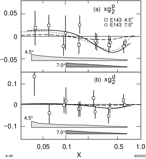
Figure 25: Data on $g_{2}$ from the SLAC E143 collaboration compared with the WW contribution and the bag model estimates of Strattmann.

His estimates of $\bar{g}_{2}$ are small compared to $g_{2}^{WW}$ and cannot be excluded by the existing data. The neutron $g_{2}$ is very small in quark and bag models for the same reason that the neutron’s $g_{1}$ is so small: the correlations of charge and spin in the $SU(6)$ symmetric neutron tend to cancel for the neutron. The second moment of $\bar{g}_{2}$ has also been estimated using QCD sum rules.[65] Surprisingly ref. [65] finds $\overline{M}_{2}[g_{2}^{\rm proton}]$ consistent with zero and $\overline{M}_{2}[g_{2}^{\rm neutron}]$ negative and significantly different from zero. Existing data cannot rule out this behavior — we shall have to wait for the HERMES facility at HERA to provide more accurate data. $\bar{g}_{2}$ depends on quark gluon correlations within the nucleon, which are not likely to be perfectly described in such simple models, so these predictions should be more as a guide than a prediction of expected behavior.

5 The Drell-Yan Process

Although deep inelastic scattering has been the source of much insight into nucleon structure, it has many limitations: polarized targets can only be probed with electromagnetic currents (neutrino scattering from polarized targets being impractical); gluon distributions do not couple directly, but instead must be inferred from careful study of the evolution of quark distributions; chiral odd distributions like $h_{1}$ decouple. None of these limitations afflict deep inelastic processes with hadron initial states. These include not only the original Drell-Yan process, $pp\rightarrow\ell\bar{\ell}+X$ via one photon annihilation, but also generalizations to annihilation via $W^{\pm}$ and $Z^{0}$, and parton-parton scattering resulting in jet production or production of hadrons or photons at high transverse momentum. QCD predictions for all of these processes are obtained by combining quark/gluon distribution and fragmentation functions with hard scattering amplitudes calculated perturbatively. This formalism is treated in standard texts — our object is to explain how the spin, twist and chirality classification developed in previous sections can be applied to Drell-Yan processes. In this section we will treat only the “classic” Drell-Yan process, $pp\rightarrow\gamma^{*}+X\rightarrow\ell\bar{\ell}+X$. The generalizations of our spin/twist/chirality analysis to other processes is fairly straightforward and yields interesting predictions for a variety of processes. The original treatment of polarized Drell-Yan at this level was made by Ralston and Soper.[43]

When last we considered Drell-Yan in §2.4, we noted that the dominance of the leading light-cone singularity could be overwhelmed by rapid phase oscillations in the matrix element. Fig. (17) shows a contribution to Drell-Yan which is obviously proportional to the product of quark distribution functions each of which has the form of eq. (3.32). Each oscillates rapidly along the light-cone $\propto e^{i\alpha P\cdot\xi}$, where $P$ is either of the two external hadron momenta. In this section we will use the formalism of the previous two sections to compute fig. (17), to show that it generates large (scaling) contributions to Drell-Yan, and to classify them with respect to spin and twist.

5.1 Operator Analysis

We begin with the Drell-Yan tensor, $W_{\mu\nu}$, from eq. (2.29), with momenta and spin more carefully labeled (and IN labels suppressed):

$$W_{\mu\nu}={s\over 2}\int d^{4}\xi e^{iq\cdot\xi}\langle P_{A}S_{A}P_{B}S_{B}|J_{\mu}(0)J_{\nu}(\xi)|P_{A}S_{A}P_{B}S_{B}\rangle.$$ (5.1)

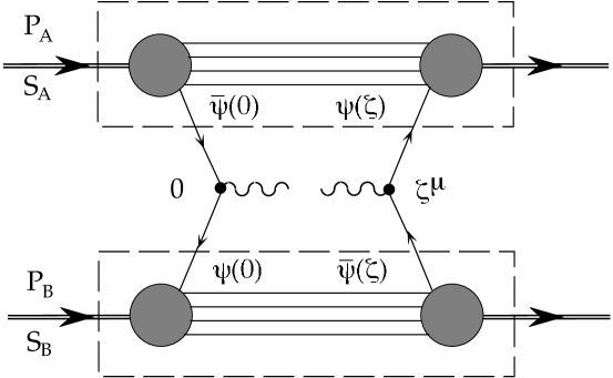
Figure 26: Dominant contribution to the Drell-Yan process.

The dominant contribution for the Drell-Yan process is shown in fig. (26). From the diagram it seems that $W_{\mu\nu}$ reduces to a product of light-cone quark correlation functions, as indicated by the markings on the figure. The essential features are 1) that nothing propagates between the two currents, so there is no singularity as $\xi^{\mu}\rightarrow 0$; and 2) each current has a quark line landing on each hadron. The latter suggests that the diagram can be factored into products of quark-hadron amplitudes by making a Fierz transformation in order to couple the spin, color and flavor indices on the quarks in a more appropriate order. First we write out the currents in terms of quark fields, limiting ourselves to terms symmetric in $\mu\leftrightarrow\nu$ (which survive contraction with the lepton tensor, $L_{\mu\nu}$),

$$J^{\{\mu}(0)J^{\nu\}}(\xi)=-\bar{\psi}_{k}(0)\psi_{l}(\xi)\bar{\psi}_{i}(\xi)\psi_{j}(0)({\bf 1}\gamma^{\{\mu})_{kj}({\bf 1}\gamma^{\nu\}})_{il}.$$ (5.2)

Note the $-$ sign from anticommuting quark fields. We wish to recouple indices so quarks acting in the same hadron are coupled to one another — $(kj)(il)\rightarrow(kl)(ij)$. The color Fierz transformation is simple,

$${\bf 1}_{kj}{\bf 1}_{il}={1\over 3}({\bf 1}_{kl}{\bf 1}_{ij}+2{\lambda^{a}_{kl}\over 2}{\lambda^{a}_{ij}\over 2}),$$ (5.3)

where ${\bf 1}$ is the $3\times 3$ unit matrix in color space. [This result is easily derived by multiplying both sides by the matrices ${\bf 1}_{kj}$ and $\lambda_{kj}$, in turn, and using multiplication properties of the $\lambda$’s.] The second term in eq. (5.3) vanishes when matrix elements are taken in color singlet hadron states. The Fierz transformation for the Dirac matrices is more complicated but better known,

$$\left(\gamma^{\{\mu}\right)_{kj}\left(\gamma^{\nu\}}\right)_{il} = {1\over 4}\Bigg{[}\left(\gamma^{\{\mu}\right)_{kl}\left(\gamma^{\nu\}}\right)_{ij}+\left(\gamma^{\{\mu}\gamma_{5}\right)_{kl}\left(\gamma^{\nu\}}\gamma_{5}\right)_{ij}$$ (5.4)

$$+ \left(\sigma^{\alpha\{\mu}\right)_{kl}\left(\sigma^{\nu\}}_{\ \alpha}\right)_{ij}\Bigg{]}+{1\over 4}g^{\mu\nu}\left[\cdots\right],$$

where the omitted terms are traces of the terms shown explicitly. One is left with bilocal light-cone correlation functions of the form: vector$\times$vector, axial vector$\times$axial vector and tensor$\times$tensor. The flavor Fierz transformation is straightforward and is left to the reader.

After reorganizing the product of currents to group fields that act in the same hadron together, the matrix element in eq. (5.1) factors into the product of quark distribution functions. However, the coordinate interval $\xi^{\mu}$ is not constrained to be lightlike. In ref. [9] each bilocal matrix element is expanded about the tangent to the light-cone defined by the large momentum $P_{A}$ or $P_{B}$, and it is shown that the light-cone contributions dominate. The matrix element in hadron $A$ is a non-trivial function of $P_{A}\cdot\xi$ along the surface $\xi^{2}=0$ and $P_{B}\cdot\xi=0$, while the matrix element in hadron $B$ is a non-trivial function of $P_{B}\cdot\xi$ along the corresponding tangent to the light-cone. We refer to ref. [9] for further details. Accepting this, $W_{\mu\nu}$ reduces to the product of quark distribution functions, one for hadron $A$, another for hadron $B$. The $V\times V$, $A\times A$, $T\times T$ structure of eq. (5.4) is reflected in the structure of the resulting product of distribution functions. The $V\times V$ part is described by:

$$W_{V}^{\mu\nu}={1\over 3}(2\pi)^{4}\delta^{2}(\vec{Q}_{\perp})\sum_{a}e_{a}^{2}f_{1}^{a}(x)f_{1}^{\bar{a}}(y)\left(p_{A}^{\mu}p_{B}^{\nu}+p_{A}^{\nu}p_{B}^{\mu}-g^{\mu\nu}p_{A}\cdot p_{B}\right),$$ (5.5)

where

$$P_{A}^{\mu} = p_{A}^{\mu}+{M^{2}\over s}p_{B}^{\mu}$$ (5.6)

$$P_{B}^{\mu} = p_{B}^{\mu}+{M^{2}\over s}p_{A}^{\mu},$$ (5.7)

with $p_{A}^{2}=p_{b}^{2}=0$ and $2p_{A}\cdot p_{B}=s$. This result is valid up to corrections of order $1/Q^{2}$ or $1/s$. There are no order $1/Q$ or $1/\sqrt{s}$ (twist-three) corrections — another example of the general result that only even twists appear in spin average deep inelastic phenomena. The $\delta(Q_{\perp}^{2})$ in eq. (5.5) reflects the fact that to leading twist and leading order in $QCD$ radiative corrections, it is as though all partons move parallel to the parent hadron. Our calculation can only be used to study observables that integrate over $\vec{Q}_{\perp}$. Eq. (5.5) is the original result of Drell and Yan: quarks that annihilate to form a virtual photon of squared-mass $Q^{2}$ and three-momentum $Q^{3}$ must have $xy=Q^{2}/s$ and $x-y=2Q^{3}/\sqrt{s}$.

In the same spirit the $A\times A$ contribution is

$$W_{A}^{\mu\nu} = -{1\over 3}(2\pi)^{4}\delta^{2}(\vec{Q}_{\perp})\Bigg{\{}\sum_{a}e_{a}^{2}g_{1}^{a}(x)g_{1}^{\bar{a}}(y){p_{A}\cdot S_{B}p_{B}\cdot S_{A}\over(p_{A}\cdot p_{B})^{2}}\left(p_{A}^{\mu}p_{B}^{\nu}+p_{A}^{\nu}p_{B}^{\mu}-g^{\mu\nu}p_{A}\cdot p_{B}\right),$$

$$+ \sum_{a}e_{a}^{2}g_{1}^{a}(x)g_{T}^{\bar{a}}(y){p_{B}\cdot S_{A}\over p_{A}\cdot p_{B}}\left(p_{A}^{\mu}S_{B\perp}^{\nu}+p_{A}^{\nu}S_{B\perp}^{\mu}\right)$$

$$+ \sum_{a}e_{a}^{2}g_{T}^{a}(x)g_{1}^{\bar{a}}(y){p_{A}\cdot S_{B}\over p_{A}\cdot p_{B}}\left(p_{B}^{\mu}S_{A\perp}^{\nu}+p_{B}^{\nu}S_{A\perp}^{\mu}\right)\Bigg{\}},$$

The first line is twist-two and contributes only when both initial hadrons are longitudinally polarized. Not surprisingly, this contribution measures $g_{1}\otimes g_{1}$. The latter two lines are twist-three, suppressed by the factor $S_{\perp}$, and contribute only when one hadron has longitudinal polarization and the other transverse. It is worthwhile relating the spin, twist and chirality structure of this result to the classification scheme developed in §’s 3 and 4. Products of the form $g_{1}\otimes g_{1}$ and $g_{1}\otimes g_{T}$ conserve quark chirality and contribute at orders of $1/Q^{2}$ which reflect the twist assignments we made in §4. Axial vector bilocals can only generate $g_{1}$ and $g_{T}$, so we can be confident that we have not missed other contributions. In fact, this result could have been written down a priori, up to coefficients of order unity simply by carefully considering the selections rules and twist assignments developed earlier in these notes. What is not at all obvious, however, is that other twist-three quark/gluon operators, of the form discussed in the previous section, and not directly related to $g_{T}$, do not arise when gluonic corrections to the diagram of fig. 26 are computed. We take up this question below.

Finally, the $T\times T$ contribution takes the form,

$$W_{T}^{\mu\nu} = -{1\over 3}(2\pi)^{4}\delta^{2}(\vec{Q}_{\perp})\Bigg{\{}\Big{[}S_{A\perp}\cdot S_{B\perp}\left(p_{A}^{\mu}p_{B}^{\nu}+p_{A}^{\nu}p_{B}^{\mu}-g^{\mu\nu}p_{A}\cdot p_{B}\right)$$

$$+ (p_{A}\cdot p_{B})\left(S_{A\perp}^{\mu}S_{B\perp}^{\nu}+S_{A\perp}^{\nu}S_{B\perp}^{\mu}\right)\Big{]}{1\over M^{2}}\sum_{a}e_{a}^{2}h_{1}^{a}(x)h_{1}^{\bar{a}}(y)$$

$$- \sum_{a}e_{a}^{2}h_{1}^{a}(x)h_{L}^{\bar{a}}(y){p_{A}\cdot S_{B}\over p_{B}\cdot p_{A}}\left(p_{A}^{\mu}S_{A\perp}^{\nu}+p_{A}^{\nu}S_{A\perp}^{\mu}\right)$$

$$- \sum_{a}e_{a}^{2}h_{L}^{a}(x)h_{1}^{\bar{a}}(y){S_{A}\cdot p_{B}\over p_{A}\cdot p_{B}}\left(p_{B}^{\mu}S_{B\perp}^{\nu}+p_{B}^{\nu}S_{B\perp}^{\mu}\right)\Bigg{\}}.$$

Here the first two lines are twist-two — they scale (modulo logarithms) in the deep inelastic limit. They contribute only when both initial hadrons are transversely polarized and provide a leading twist probe of transversity distributions. The second two lines are twist-three and contribute when one hadron is transversely polarized and the other longitudinally. Once again the classification scheme of §’s 3 and 4 is illustrated. Note, for example, that transverse-longitudinal polarization receives contributions from both $g_{1}\otimes g_{T}$ and $h_{1}\otimes h_{L}$.

Unfortunately things are not quite as simple as they have been presented so far. Two questions of gauge invariance arise — one straightforward and the other rather subtle:

• The factorization of $W_{\mu\nu}$ into products of bilocal operators acting in different hadrons is not color gauge invariant. Evidence of this is the absence of the Wilson link,

  $${\cal P}\left(\exp i\int_{0}^{\xi}d\zeta^{\mu}A_{\mu}(\zeta)\right)$$ (5.10)

  between the quark fields at $0$ and $\xi$. The problem is that we have not included those diagrams that represent each quark propagating in the color field of the remnants of the other hadron. The same problem was discussed in §3 for the case of deep inelastic scattering, where it is easier to handle because the operator product expansion will preserve gauge invariance if treated with sufficient care. In this case we must find and analyze the diagrams which restore color gauge invariance through twist-three and be certain that they do not generate any contributions to $W_{\mu\nu}$ beyond rendering the identification of Drell-Yan matrix elements with quark distributions functions gauge invariant. An example of the type of diagram that does the trick is shown in fig. (27). The interested reader is referred to ref. [9] for details.

• The results we have just quoted (eqs. (5.1), (5.5), and (5.1)) violate electromagnetic gauge invariance at twist-three. It is easy to see that the twist-three terms do not satisfy $W_{\mu\nu}q^{\nu}=0$. Once again the answer lies in diagrams like fig. (27). In this case, when the Wilson link which appears in the bilocal operator is expanded to first order away from the light-cone, a set of contributions with explicit transverse gluon fields arise. Using the equations of motion these can be related back to the product of good and bad quark fields which define the twist-three distributions $g_{T}$ and $h_{L}$. With sufficient care one finds exactly the terms necessary to restore electromagnetic gauge invariance. Once again a fuller discussion can be found in ref. [9].

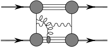
Figure 27: New class of diagrams, needed to restore color and electromagnetic gauge invariance.

5.2 Polarized Drell-Yan: a Brief Summary

Since the equations and the analysis in this section have become rather complicated, it is useful to extract the simple predictions for spin asymmetries to provide a summary and to reference the workers who originally derived these results.

In the polarized Drell-Yan process, three cases appear: longitudinal-longitudinal ($LL$), transverse-transverse ($TT$) and longitudinal-transverse ($LT$), as illustrated in fig. (28). If instead of virtual photon production, we had considered Drell-Yan production of $Z^{0}$ or $W^{\pm}$, then a longitudinal, leading twist, parity violating single spin asymmetry proportional to $g_{1}\otimes f_{1}$ appears. There is no analogous transverse asymmetry because the product $h_{1}\otimes f_{1}$ cannot conserve quark chirality.

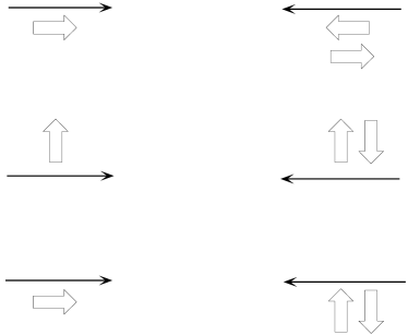
Figure 28: Various polarization configurations, studied in the Drell-Yan process. The small arrows denote the spin projections of the two nucleons relative to the direction of the nucleon beams (long arrows). For one of the nucleons the difference of the up and down projections is taken. One distinguishes longitudinal (top), transverse (middle) and longitudinal-transverse (bottom) scattering.

The longitudinal asymmetry, which was first studied by Close and Sivers [66], is given by:

$$A_{LL}={\sum_{a}e_{a}^{2}g_{1}^{a}(x)g_{1}^{\bar{a}}(y)\over\sum_{a}e_{a}^{2}f_{1}^{a}(x)f_{1}^{\bar{a}}(y)}.$$ (5.11)

Ralston and Soper first discovered transversity, defined a twist-two distribution and expressed the transverse asymmetry as:[43]

$$A_{TT}={\sin^{2}\theta\ \cos 2\phi\over 1+\cos^{2}\theta}{\sum_{a}e_{a}^{2}h_{1}^{a}(x)h_{1}^{\bar{a}}(y)\over\sum_{a}e_{a}^{2}f_{1}^{a}(x)f_{1}^{\bar{a}}(y)}.$$ (5.12)

The angles are defined in the lepton center of mass frame. The longitudinal-transverse asymmetry has been investigated by Jaffe and Ji [9] and can be written as:

$$A_{LT}={2\sin 2\theta\cos\phi\over 1+\cos^{2}\theta}{M\over\sqrt{Q^{2}}}{\sum_{a}e_{a}^{2}(g_{1}^{a}(x)yg_{T}^{\bar{a}}(y)-xh_{L}^{a}(x)h_{1}^{\bar{a}}(y))\over\sum_{a}e_{a}^{2}f_{1}^{a}(x)f_{1}^{\bar{a}}(y)}.$$ (5.13)

Clearly, it is a twist-three observable, which in principle allows for a measurement of $h_{L}$.

6 Annihilation and Quark Fragmentation
Functions

As a final application we give a brief introduction to the classification and uses of the spin dependent fragmentation functions which determine the distribution of final state hadrons in deep inelastic processes. There are strong reasons to want to develop a better understanding of hadron fragmentation processes. In §1 we mentioned the possibility of studying the spin structure of unstable hadrons like the $\Lambda,\rho$ and $D^{*}$. Another reason is that parity violating processes like $W^{\pm}\rightarrow q\bar{q}\rightarrow$ hadrons provide probes of spin structure unavailable in deep inelastic scattering, where the analogous experiment would be neutrino scattering from a polarized target. A final reason is that the selection of a particular hadronic fragment can serve as a filter for an interesting quark or gluon distribution function. The material in this section is based primarily on refs. [10, 67] and [68] where more details can be found.

6.1 Single Particle Inclusive Annihilation

The simplest quark fragmentation function is represented diagrammatically in fig. (29).

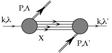
Figure 29: Quark fragmentation function in a helicity basis.

More complicated fragmentation processes, such as coherent fragmentation of several quarks and gluons, do not contribute until order $1/Q^{2}$, beyond our interest. First we consider the helicity classification in analogy to §4.1–4.3. In the figure a quark of momentum $k$ and helicity $\lambda$ fragments into a hadron of momentum $P$ and helicity $\Lambda$ plus an unobserved final state $X$. The process then repeats in reverse as the unobserved system, $X$, plus the hadron of momentum $P$ and helicity $\Lambda^{\prime}$ reconstitute the quark of momentum $k$ and helicity $\lambda^{\prime}$. The scattering $k+P\to k+P$ is forward, i.e. collinear. For definiteness, we take the momentum of the quark–hadron system to be aligned along the $\hat{e}_{3}$–axis. Then helicity is conserved as a consequence of angular momentum conservation about this axis: $\lambda-\Lambda=\lambda^{\prime}-\Lambda^{\prime}$. As in deep inelastic scattering, the initial and final hadron helicities $\Lambda$ and $\Lambda^{\prime}$ need not be equal because the hadron need not have been in a helicity eigenstate; likewise for the quark. As in scattering, the quark lines may correspond either to good or bad light-cone components.

Some of the results of refs. [11] and [67] are as follows. Quark fragmentation functions of the form shown in fig. (29) and the equivalent gluon fragmentation functions (without further active parton lines) are sufficient to characterize hadron production in hard processes, provided: i) one studies leading twist (${\cal O}(1/Q^{0})$) in any hard process, or ii) one studies an effect in deep inelastic lepton scattering at the lowest twist at which it arises, and one ignores QCD radiative corrections.[67] Each appearance of a bad component of the quark field costs one power of $\sqrt{Q^{2}}$ in the deep inelastic limit (i.e. it increases the twist by unity). As in scattering, for produced hadrons of spin-1/2, helicity differences are observed in longitudinal spin asymmetries; helicity flip is observed in transverse spin asymmetries. Since perturbative QCD cannot flip quark chirality (except through quark mass insertions which we assume to be negligible for light quarks), chirally–odd quark distribution and fragmentation functions must occur in pairs.

Fragmentation functions can be labeled uniquely by specifying the helicity of quarks and hadrons and the light-cone projection of the quarks in direct analogy to the classification of distribution functions. We denote fragmentation functions in a helicity basis by $\hat{\cal A}$. Parity invariance of QCD requires: $\hat{\cal A}_{\lambda\Lambda,\lambda^{\prime}\Lambda^{\prime}}=\hat{\cal A}_{-\lambda-\Lambda,-\lambda^{\prime}-\Lambda^{\prime}}$. Time reversal invariance, which further reduces the number of independent quark distribution functions does not generate relationships among the $\{\hat{\cal A}\}$ because it changes the out–state $(PX)_{\rm out}$ in fig. (29) to an in–state. As in the scattering case, we denote the appearance of bad light-cone components by an asterix on the appropriate helicity index.

As a simple example, consider production of a scalar meson like the pion. Through order $1/\sqrt{Q^{2}}$ there are three independent fragmentation functions: $\hat{\cal A}_{{1\over 2}0,{1\over 2}0}$, $\hat{\cal A}_{{1\over 2}0,{1\over 2}^{*}0}$, and $\hat{\cal A}_{{1\over 2}^{*}0,{1\over 2}0}$. The first is twist-two and scales in the $Q^{2}\rightarrow\infty$ limit, the latter two are twist-three and are suppressed by $1/\sqrt{Q^{2}}$ in the $Q^{2}\rightarrow\infty$ limit. The first function, $\hat{\cal A}_{{1\over 2}0,{1\over 2}0}$, is proportional to the traditional fragmentation function $D(z,Q^{2})$. It has the same twist, light-cone, helicity and chirality structure as $f_{1}(x,Q^{2})$, so to avoid an explosion of notation we denote it by $\hat{f}_{1}(z,Q^{2})$ [We will follow the same convention for other fragmentation functions.]:

$$\hat{f}_{1}(z,Q^{2})\propto\hat{\cal A}_{{1\over 2}0,{1\over 2}0}$$ (6.1)

If we were studying quark distribution functions, the other two helicity amplitudes would be equal by time-reversal invariance. Here, there are two independent fragmentation functions.

$$\hat{e}_{1}(z,Q^{2}) \propto \hat{\cal A}_{{1\over 2}0,{1\over 2}^{*}0}+\hat{\cal A}_{{1\over 2}^{*}0,{1\over 2}0}$$

$$\hat{e}_{\bar{1}}(z,Q^{2}) \propto \hat{\cal A}_{{1\over 2}0,{1\over 2}^{*}0}-\hat{\cal A}_{{1\over 2}^{*}0,{1\over 2}0}$$

We have found that the helicity classification of fragmentation functions is identical to that of distribution functions at leading twist. At twist-three, however, there are more fragmentation functions due to the absence of time reversal constraints.

The application to spin–$1/2$ is analogous to the classification of spin–$1/2$ distribution functions given in Table 2 of §4.2.2 except that each twist-three fragmentation function comes in two forms, one even and the other odd under time reversal. We suspect that the T-even functions are more important than the T-odd since the latter vanish in the absence of final state interactions. So fragmentation at twist-two requires $\hat{f}_{1}(z)$, $\hat{g}_{1}(z)$ and $\hat{h}_{1}(z)$ with helicity, transversity and chirality properties identical to the analogous distribution function. The only twist-three fragmentation function likely to be of much interest is the spin-averaged, chiral-odd, time reversal even function $\hat{e}_{1}(z)$.

In order to relate particular deep inelastic processes to quark distribution and fragmentation functions and to study them in models of non-perturbative QCD, it is necessary to have operator representations for them. This formalism is developed in refs. [11, 67]. Here we display the results for the three leading twist fragmentation functions for a spin-$1/2$ hadron, and for the twist-three spin average function, $\hat{e}_{1}$. Generalizations to spin-$1$ can be found in ref. [67]. The generic expression for a fragmentation function takes the form,

$$\hat{\Gamma}(z)={\rm Tr}\left\{\Gamma_{\alpha\beta}\sum_{X}\int\frac{d\lambda}{2\pi}e^{-i\lambda/z}\left<0|\psi_{\beta}(0)|PX\right>\left<PX|\bar{\psi}_{\alpha}(\lambda n)|0\right>\right\}.$$ (6.3)

where $\Gamma_{\alpha\beta}$ stands for an arbitrary Dirac matrix. This result holds under the condition that the diagram of fig. (29) dominates. To obtain $\hat{f}_{1}$, $\hat{g}_{1}$ and $\hat{h}_{1}$ one chooses $\Gamma=n/,n/\gamma_{5}$ and $\sigma^{j}_{\nu}n^{\nu}i\gamma_{5}$ respectively,

$$\hat{f}_{1}(z) = \frac{1}{2}\sum_{X}\int\frac{d\lambda}{2\pi}e^{-i\lambda/z}\left<0|n/\psi(0)|PX\right>\left<PX|\bar{\psi}(\lambda n)|0\right>,$$

$$\hat{g}_{1}(z) = \frac{1}{2}\sum_{X}\int\frac{d\lambda}{2\pi}e^{-i\lambda/z}\left<0|n/\gamma_{5}\psi(0)|PSX\right>\left<PSX|\bar{\psi}(\lambda n)|0\right>,$$

$$\frac{S_{\perp}{{}^{j}}}{M}\hat{h}_{1}(z) = \frac{1}{2}\sum_{X}\int\frac{d\lambda}{2\pi}e^{-i\lambda/z}\left<0|\sigma^{j}_{\nu}n^{\nu}i\gamma_{5}\psi(0)|PS_{\perp}X\right>\left<PS_{\perp}X|\bar{\psi}(\lambda n)|0\right>$$

At twist-three the equations of motions can be used to express the structure functions in terms of independent degrees of freedom, quantized at $\xi^{+}=0$. For example one can obtain two expressions for the chiral odd, T-even spin independent fragmentation function $\hat{e}_{1}(z)$. One involving $\psi\bar{\psi}$ and another where bad light-cone components have been traded for transverse derivatives and gluon degrees of freedom,

$$M\hat{e}_{1}(z) = \frac{1}{2}\sum_{X}\int\frac{d\lambda}{2\pi}e^{-i\lambda/z}\langle 0|\psi(0)|PX\rangle\langle PX|\bar{\psi}(\lambda n)|0\rangle$$

$$\hat{e}_{1}(z) = \frac{z}{4M}\sum_{X}\int\frac{d\lambda}{2\pi}e^{-i\lambda/z}\{\langle 0|in/D/_{\perp}(0)\psi_{+}(0)|PX\rangle\langle PX|\bar{\psi}_{+}(\lambda n)|0\rangle$$

$$- \langle 0|\psi_{+}(0)|PX\rangle\langle PX|\bar{\psi}_{+}(\lambda n)iD/_{\perp}(\lambda n)n/|0\rangle\}.$$

With these ingredients we are now prepared to explore a few applications of spin dependent fragmentation functions.

6.2 Polarized $q\rightarrow\Lambda$ Fragmentation Functions from $e^{+}e^{-}\to\Lambda+X$

This section is based on work done with M. Burkardt.[68] In the symmetric quark model, the $\Lambda$-baryon has a rather simple spin-flavor wavefunction. All its spin is carried by the $s$-quark, while the $ud$-pair is coupled to $S=0$, $I=0$: $\Delta u^{\Lambda}=\Delta d^{\Lambda}=0$ and $\Delta s^{\Lambda}=1$. While the quark model identifies the $\Lambda$-spin with the spin of the $s$-quark, the data on the quark spin structure of the nucleon suggests that the actual situation is more complex. If we take the latest SMC/SLAC data on the $\int_{0}^{1}dxg_{1}^{ep}(x)$, combine it with $\beta$-decay data and assume exact $SU(3)_{flavor}$ symmetry for baryon axial charges, we find

$$\Delta u^{\Lambda}=\Delta d^{\Lambda} = {1\over 3}(\Sigma-D)=-0.23\pm 0.06$$

$$\Delta s^{\Lambda} = {1\over 3}(\Sigma+2D)=+0.58\pm 0.07$$

It would be exciting to test the $SU(3)_{flavor}$ assumption by observing deep inelastic scattering from a $\Lambda$ target. Unfortunately we have to settle for observing the $\Lambda$ as a fragment in annihilation processes. The parity violating, self analyzing decay of the final state $\Lambda$ makes it particularly easy to study its polarization in fragmentation processes. Measurement of the helicity asymmetries for semi-inclusive production of $\Lambda$’s in $e^{+}e^{-}$ annihilation near the $Z^{0}$ resonance allows a complete determination of the spin-dependent fragmentation functions for the different quark flavors into the $\Lambda$. In the event that these could be measured it would be very interesting to compare the spin fractions measured in fragmentation, $\Delta\hat{s}^{\Lambda}$, $\Delta\hat{d}^{\Lambda}$, and $\Delta\hat{u}^{\Lambda}$, with the predictions, eq. (LABEL:lambdaspin) in order to get a better understanding of the role of spin in the fragmentation process.

We are concerned here with twist-two helicity asymmetries, described by the fragmentation function $\hat{g}_{1}(z,Q^{2})$. For simplicity we adopt a more conventional parton-model notation where we define $d^{\Lambda(L)}_{q(L)}$ to be the probability that a left handed $\Lambda$ fragments into a left handed quark, etc. Then the unpolarized differential cross section for $e^{-}e^{+}\rightarrow\Lambda+X$ is obtained by summing over the cross sections for $e^{+}e^{-}\rightarrow q\bar{q}$, weighted with the probability $d^{\Lambda}_{q}(z,Q^{2})$ that a quark with momentum ${1\over z}P$ fragments into a $\Lambda$ with momentum $P$. As usual, we suppress the $Q^{2}$ dependence generated by radiative corrections in QCD,

$${d^{2}\sigma^{\Lambda}\over d\Omega\,dz}=\sum_{q}{d\sigma^{q}\over d\Omega}d^{\Lambda}_{q}(z).$$ (6.7)

There is a single polarized fragmentation function for each flavor of quark or antiquark,

$$\Delta\hat{q}(z) = d^{\Lambda(L)}_{q(L)}(z)-d^{\Lambda(R)}_{q(L)}(z)$$

$$= d^{\Lambda(L)}_{q(L)}(z)-d^{\Lambda(L)}_{q(R)}(z)$$

$$\Delta\hat{\bar{q}}(z) = d^{\Lambda(L)}_{\bar{q}(L)}(z)-d^{\Lambda(R)}_{\bar{q}(L)}(z)$$ (6.8)

$$= d^{\Lambda(L)}_{\bar{q}(L)}(z)-d^{\Lambda(L)}_{\bar{q}(R)}(z),$$

and furthermore isospin invariance requires that $\Delta\hat{u}(z)=\Delta\hat{d}(z)$ and $\Delta\hat{\bar{u}}(z)=\Delta\hat{\bar{d}}(z)$, so the number of independent fragmentation functions is reduces to four — e.g. $\Delta{\hat{u}},\Delta{\hat{\bar{u}}},\Delta{\hat{s}}$ and $\Delta{\hat{\bar{s}}}$.

As an example we quote the prediction for $\Lambda$ production in $e^{-}e^{+}$ annihilation via photons. In this case one has to start from polarized $e^{-}$ (or $e^{+}$) in order to fix the polarization of the quarks. One finds for the helicity asymmetric cross-section,

$${d^{2}\sigma^{e^{-}(L)e^{+}\rightarrow\Lambda(L)X}\over d\Omega\,dz}-{d^{2}\sigma^{e^{-}(L)e^{+}\rightarrow\Lambda(R)X}\over d\Omega\,dz}={\alpha^{2}\over 2s}\cos\theta\left[{5\over 9}\left(\Delta\hat{u}(z)+\Delta\hat{\bar{u}}(z)\right)+{1\over 9}\left(\Delta\hat{s}(z)+\Delta\hat{\bar{s}}(z)\right)\right]$$ (6.9)

where $L,R$ denotes the helicity of the $e^{-}$ and the $\Lambda$. So annihilation into a single photon allows one combination of the four independent fragmentation functions to be measured. As described in ref. [68], annihilation at the $Z^{0}$ and just off the $Z^{0}$ peak where $\gamma-Z$ interference is largest will allow independent detection of all four quark and antiquark fragmentation functions. For further discussion of this process, backgrounds and experimental possibilities see ref. [68] and recent papers by the $Aleph$ and $Delphi$ collaborations.

6.3 Observing $h_{1}(x,Q^{2})$ in Electroproduction

This section is based on work done with X. Ji.[10, 67] Chirally odd quark distributions are difficult to measure because they are suppressed in totally–inclusive deep inelastic scattering. So far, the only practical way to determine $h_{1}(x,Q^{2})$ we have discussed has been Drell-Yan production with transversely polarized target and beam.

As an application of the fragmentation function formalism – one of many – we show how a chirally odd fragmentation function can be exploited to enable a measurement of $h_{1}(x,Q^{2})$ to be obtained in polarized electroproduction of pions from a transversely polarized nucleon. This is an experiment which could be performed at several existing facilities. Related suggestions involving semi–inclusive production of $\Lambda$–hyperons and of two pions have been discussed previously.[69, 42] The proposal outlined here is simpler since it involves only one particle in the final state and does not require measurement of that particle’s spin. The price we pay for this simplicity is suppression by a power of $\sqrt{Q^{2}}$.

We consider pion production in the current fragmentation region of deep-inelastic scattering with longitudinally polarized leptons on a polarized nucleon target. The simplest diagram for the process is shown in fig. (30), where a quark struck by the virtual photon fragments into an observed pion plus other unobserved hadrons. The cross section is proportional to a trace and integral over the quark loop which contains the quark distribution function and fragmentation function. Due to chirality conservation at the hard (photon) vertex, the trace picks up only the products of the terms in which the distribution and fragmentation functions have the same chirality. When the nucleon is longitudinally polarized (with respect to the virtual-photon momentum), the twist-two, chirally even distribution $g_{1}(x)$ can couple with the twist-two chirally even fragmentation function $\hat{f}_{1}(z)$, producing a leading contribution ${\cal O}(1/Q^{0})$ to the cross section. On the other hand, in the case of a transversely polarized nucleon, there is no leading-order contribution. At the next order, the nucleon’s transversity distribution $h_{1}(x)$ can combine with the twist-three chirally odd fragmentation function $\hat{e}_{1}(z)$, and similarly $g_{T}(x)$ can combine with the chirally even transverse-spin distribution $\hat{f}_{1}(z)$. Both couplings produce $1/\sqrt{Q^{2}}$ contributions to the cross section.

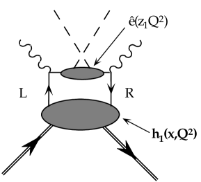
Figure 30: Single particle inclusive scattering $ep\rightarrow ehX$. The labels $L$ and $R$ reflect the chiral odd nature of $h_{1}$.

It is simple to see, however, that fig. (30) alone does not produce an electromagnetically-gauge-invariant result. This is a typical example of the need to consider multi-quark/gluon processes beyond twist-two. In the present case (twist-three), however, the contributions from coherent scattering can be expressed, with novel use of QCD equations of motion, in terms of the distributions and fragmentation functions defined from quark bilinears. This is a specific example of another rule quoted in §6.2: “Parton diagrams (without further active parton lines) are sufficient to characterize hadron production in hard processes, provided: one studies an effect in deep inelastic lepton scattering at the lowest twist at which it arises, and one ignores QCD radiative corrections.” The combined result is gauge invariant, as can be seen from the resulting nucleon tensor,

$$\hat{W}^{\mu\nu}=-i\epsilon^{\mu\nu\alpha\beta}{q_{\alpha}\over\nu}[(S\cdot n)p_{\beta}\hat{G}_{1}(x,z)+{S_{\perp\beta}}\hat{G}_{T}(x,z)]$$ (6.10)

The two structure functions in $\hat{W}^{\mu\nu}$ are related to parton distributions and fragmentation functions,

$$\hat{G}_{1}(x,z) = {1\over 2}\sum_{a}e_{a}^{2}g_{1}^{a}(x)\hat{f}_{1}^{a}(z)$$

$$\hat{G}_{T}(x,z) = {1\over 2}\sum_{a}e_{a}^{2}\Big{[}g^{a}_{T}(x)\hat{f}^{a}_{1}(z)+{h^{a}_{1}(x)\over x}{\hat{e}^{a}(z)\over z}\Big{]}$$

where the summation over $a$ includes quarks and antiquarks of all flavors.

To isolate the spin-dependent part of the deep-inelastic cross section we take the difference of cross sections with left-handed and right-handed leptons, we use

$${d^{2}\Delta\sigma\over dE^{\prime}d\Omega}={\alpha_{\rm em}^{2}\over Q^{4}}{E^{\prime}\over EM_{N}}\Delta\ell^{\mu\nu}\hat{W}_{\mu\nu}$$ (6.12)

It is convenient to express the cross section in terms of scaling variables in a frame where lepton beam defines the $\hat{e}_{3}$-axis and the $\hat{e}_{1}-\hat{e}_{3}$ plane contains the nucleon polarization vector, which has a polar angle $\alpha$. In this system, the scattered lepton has polar angles $(\theta,\phi)$ and therefore the momentum transfer ${\bf q}$ has angles $(\theta,\pi-\phi)$. Then we obtain an expression for the semi-inclusive process quite similar to that for the total inclusive scattering defined by eq. (LABEL:eq:spindepxsection).

$${d^{4}\Delta\sigma\over dx\,dy\,dz\,d\phi} = {8\alpha^{2}_{\rm em}\over Q^{2}}\Big{[}\cos\alpha(1-{y\over 2})G_{1}(x,z)$$

$$+ \cos\phi\sin\alpha\sqrt{(\kappa-1)(1-y)}\left(G_{T}(x,z)-G_{1}(x,z)(1-{y\over 2})\right)\Big{]}$$

where $\kappa=1+4x^{2}M^{2}/Q^{2}$ in the second term signals the suppression by a factor of $1/\sqrt{Q^{2}}$ associated with the structure function $G_{T}$. The existence of $G_{1}$ in the same term is due to a small longitudinal polarization of the nucleon relative to ${\bf q}$ when its spin is perpendicular to the lepton beam.

Eq. (LABEL:eq:final) is the main result of this section. As a check, we multiply by $z$, integrate over it and sum over all hadron species. Using the well-known momentum sum rule,

$$\sum_{\rm hadrons}\int dzz\hat{f}_{1}^{a}(z)=1,$$ (6.14)

and the sum rule,

$$\sum_{\rm hadrons}\int dz\hat{e}^{a}_{1}(z)=0$$ (6.15)

which is related to the fact that the chiral condensate vanishes in the perturbative QCD vacuum, we get the result for total inclusive scattering, given in eq. (LABEL:eq:spindepxsection) The similarity between the inclusive and semi-inclusive cross sections suggests that they can be extracted conveniently from the same experiment.

The aim of this example was to show that an unfamiliar fragmentation function ($\hat{e}_{1}$) could be employed to obtain a measurement of an interesting, if unfamiliar, distribution function ($h_{1}$). It is apparent from eq. (LABEL:eq:final) that we have been only partially successful: although the $h_{1}^{a}$ distribution for each quark flavor appears in eq. (LABEL:eq:final), the sum over flavors couples it to the unknown flavor dependence of $\hat{e}_{1}^{a}$. Perhaps flavor tagging can be used at large–$z$ to identify the contributions of individual quark flavors. For $x$ in the valence region (where one can ignore antiquarks in the nucleon), and $z\rightarrow 1$, the dominant fragmentation, $u\rightarrow\pi^{+}$, $d\rightarrow\pi^{-}$, $s\rightarrow K^{-}$, may allow one to trigger on the contributions of $u$, $d$ and $s$ quarks separately.[70] One might be concerned that the unknown fragmentation function, $\hat{e}_{1}$, might not respect the dominant fragmentation selection rules, which have only been tested for the spin-averaged, twist-two fragmentation function, $\hat{f}_{1}$. However, the coherent gluon interactions which distinguish the twist-three $\hat{e}_{1}$ from $\hat{f}_{1}$ are flavor independent and should not alter the selection rules. Although this may be a difficult path to measuring $h_{1}$, so are all the others. This one owes its existence to our improved understanding of the spin and twist dependence of quark fragmentation functions, including the spin-average twist-three fragmentation function $\hat{e}_{1}$.

References

- [1] I. J. R. Aitchison, A. J. G. Hey, Gauge Theories in Particle Physics, 2nd Edition (Adam Hilger, Bristol, 1989).
- [2] F. E. Close, An Introduction to Quarks and Partons (Academic Press, London, 1979).
- [3] O. Nachtmann, Elementary Particle Physics (Springer-Verlag, Berlin, 1990)
- [4] J. Collins, Renormalization (Cambridge University Press, Cambridge, 1984).
- [5] T. Muta, Foundations of Quantum Chromodynamics (World Scientific, Singapore, 1987).
- [6] R. G. Roberts, The Structure of the Proton (Cambridge University Press, Cambridge, 1990).
- [7] R. L. Jaffe and X. Ji, Phys. Rev. D43 (1991) 724.
- [8] R. L. Jaffe and X. Ji, Phys. Rev. Lett. 67 (1991) 552.
- [9] R. L. Jaffe and X. Ji, Nucl. Phys. B375 (1992) 527.
- [10] R. L. Jaffe and X. Ji, Phys. Rev. Lett. 71 (1993) 2547.
- [11] K. Chen, G. R. Goldstein, R. L. Jaffe and X. Ji, Nucl. Phys. B445 (1995) 380.
- [12] G. R. Goldstein, R. L. Jaffe and X. Ji, Phys. Rev. D52 (1995) 5006.
- [13] H1 Collaboration, Phys. Lett. B324 (1994) 241; ZEUS Collaboration, Phys. Rev. Lett. 75 (1995) 1006.
- [14] C. G. Callan and D. J. Gross, Phys. Rev. Lett. 22 (1969) 156.
- [15] R. L. Jaffe, Comm. Nucl. Part. Phys. 14 (1990) 239.
- [16] S. G. Gorishny, A. L. Kataev, S. A. Larin Phys. Lett. B259 (1991) 144.
- [17] G. Bunce, J. Collins, S. Heppelmann, R. L. Jaffe, S. Y. Lee, Y. Makdisi, R. W. Robinett, J. Soffer, M. Tannenbaum, D. Underwood, A. Yokosawa, Particle World 3 (1992) 1.
- [18] R. L. Jaffe, in Relativistic Dynamics and Quark–Nuclear Physics, M. B. Johnson and A. Picklesimer, eds. (Wiley, New York, 1986).
- [19] R. K. Ellis, W. Furmanski, and R. Petronzio, Nucl. Phys. B207 (1982) 1, ibid. B212 (1983) 29.
- [20] C. Itzykson and J. B. Zuber, Quantum Field Theory (McGraw–Hill, New York, 1980).
- [21] S. Coleman, Aspects of Symmetry (Cambridge, 1985).
- [22] B. L. Ioffe, it JETP Lett. 9 (1969) 163; 10 (1969) 143; Phys. Lett. 30B (1969) 123.
- [23] R. L. Jaffe, Phys. Rev. D5 (1972) 2622; and in Proceedings of the 1972 Erice School — Highlights in Particle Physics, A. Zichichi, ed. (Edetrice Compositori, Bologna, 1973).
- [24] J. D. Bjorken, Phys. Rev. Lett. 16 (1966) 408.
- [25] K. Johnson and F. E. Low, Prog. Theor. Phys. Suppl. 37 (1967) 74.
- [26] J. Ellis and R. L. Jaffe, Scaling, Short Distances and the Light Cone, Notes based on lectures presented at Univ. of Calif. Santa Cruz Summer School on Particle Physics, 1973, SLAC-PUB-1353, Dec 1973, unpublished.
- [27] D. Broadhurst, J. Gunion and R. L. Jaffe, Phys. Rev. D8 (1973) 566; Ann. Phys. 81 (1973) 88.
- [28] J. D. Bjorken and S. D. Drell, Relativistic Quantum Field Theory (McGraw Hill, New York, 1964).
- [29] T. P. Cheng and L. F. Li, Gauge Theory of Elementary Particle Physics (Clarendon Press, Oxford, 1984).
- [30] J. C. Collins, D. E. Soper, Nucl. Phys. B194 (1982) 445.
- [31] N. N. Bogolyubov and D. V. Shirkov, Introduction to the Theory of Quantized Fields (Wiley Interscience, New York, 1959).
- [32] R. K. Ellis, H. Georgi, M. Machacek, H. D. Politzer, G. G. Ross, Phys. Lett. 78B (1978) 281; Nucl. Phys. B152 (1979) 285.
- [33] H. Fritzsch and M. Gell-Mann, in Broken Scale Invariance and the Light-Cone 1971 Coral Gables Conference on Fundamental Interactions at High Energies, M. Dal Cin, G. J. Iverson and A. Perlmutters, eds. (Gordon and Greach, New York, 1971).
- [34] P. Hoodbhoy, A. V. Manohar and R. L. Jaffe, Nucl. Phys. B312 (1989) 571.
- [35] R. L. Jaffe and A. V. Manohar, Nucl. Phys. B321 (1989) 343; E. Sather and C. Schmidt Phys. Rev. D42 (1990) 1424.
- [36] S. Weinberg, Phys. Rev. 150 (1966) 1313.
- [37] L. Susskind, Phys. Rev. 165 (1968) 1535.
- [38] J. Kogut and D. E. Soper, Phys. Rev. D1 (1970) 2901.
- [39] R. L. Jaffe and M. Soldate, in Perturbative Quantum Chromodynamics (Tallahassee, 1981), D. W. Duke and J. F. Owens, eds.; Phys. Rev. D26 (1982) 49.
- [40] R. L. Jaffe, Phys. Lett. 116B (1982) 437; Nucl. Phys. B229 (1983) 205.
- [41] R. L. Jaffe and A. V. Manohar, Phys. Lett. B223 (1989) 218.
- [42] X. Artru and M. Mekhfi, Z. Phys. C45 (1990) 669.
- [43] J. Ralston and D. E. Soper, Nucl. Phys. B152 (1979) 109.
- [44] R. P. Feynman, Photon-hadron Interactions, (Benjamin, Reading, 1972).
- [45] R. G. Roberts J. D. Jackson and G. G. Ross. Phys. Lett. B226 (1989) 159.
- [46] J. Soffer, Phys. Rev. Lett. 74 (1995) 1292.
- [47] B. Kamal, A. P. Contogouris, and Z. Merebashvili, McGill University preprint, 1995.
- [48] K. Sasaki J. Kodaira, S. Matusa and T. Uematsu, Nucl. Phys. B159 (1979) 99.
- [49] J. Kodaira, Nucl. Phys. B165 (1979) 129.
- [50] S. Wandzura and F. Wilczek, Phys. Lett. 72B (1977) 195.
- [51] E. V. Shuryak and A. I. Vainstein, Nucl. Phys. B201 (1982) 141.
- [52] H. Burkhardt and W. N. Cottingham, Ann. Phys. 56 (1970) 453.
- [53] G. C. Fox and D. Z. Freedman, Phys. Rev. 182 (1969) 1628.
- [54] I. Antoniadis and C. Kounnas, Ecôle Polytechnique preprint A399.0580 (1980), unpublished.
- [55] M. Burkardt, University of Washington Preprint, May 1995, hep-ph/9505226.
- [56] G. Altarelli, B. Lampe, P. Nason, and G. Ridolfi, Phys. Lett. B334 (1994) 187.
- [57] M. A. Ahmed and G. G. Ross, Phys. Lett. B56 (1975) 385; Nucl. Phys. B111 (1976) 441.
- [58] P. G. Ratcliffe Nucl. Phys. B264 (1986) 493.
- [59] A. P. Bukhvostov, E. A. Kuraev and L. N. Lipatov, JETP Letters 37 (1983) 483.
- [60] X. Ji and C. Chou, Phys. Rev. D42 (1990) 3637.
- [61] Y. Yasui, Prog. Theor. Phys. Suppl. 120 (1995) 239, and references therein.
- [62] A. Ali, V. Braun and G. Hiller, Phys. Lett. B226 (1991) 117.
- [63] K. Abe, et al. The E143 Collaboration, SLAC-Pub-95-6982, August 1995.
- [64] M. Strattman, Z. Phys. C60 (1995) 369.
- [65] I. I. Balitsky, V. M. Braun, and A. V. Kolesnichenko, Phys. Lett. B242 (1990) 245; E. Stein, P. Gornicki, L. Mankiewicz, A. Schafer, and W. Greiner, Phys. Lett. B343 (1995) 369.
- [66] F. E. Close and D. Sivers, Phys. Rev. Lett. 39 (1977) 1116.
- [67] X. Ji, Phys. Rev. D49 (1994) 114.
- [68] M. Burkardt and R. L. Jaffe, Phys. Rev. Lett.70 (1993) 2537.
- [69] J. C. Collins, S. F. Heppelmann, G. A. Ladinsky, Nucl. Phys. B420 (1994) 565.
- [70] M. Veltri, M. Dueren, K. Rith, L. Mankiewicz, A. Schaefer, in Proceedings of the Workshop on Physics at HERA vol. 1, 447, W. Buchmuller and G. Ingelman, eds., 1992.