Abstract

We extend the ‘topological inflation’ of Linde and Vilenkin to unstable monopoles. This allows the monopole to decay; not inflating eternally, as topological inflation demands. Such a situation happens naturally in some Grand Unified Theories — such as supersymmetric flipped-$SU(5)$. We analyse analytically the dynamics of inflating monopoles to determine the equations governing the expansion, additionally recovering the bound on the scale of symmetry breaking found numerically by Sakai et. al. The latter half of this paper is devoted to the Cosmology of inflating unstable monopoles — which is an example of an inhomogeneous cosmology. We describe how such a monopole may be formed and how long it inflates for — finding it to be a random process. We then derive how cosmological parameters, such as density and temperature, are distributed at the end of inflation, and how the Universe reheats as the monopole decays. The general conclusion of this work is that such inflation creates a local region of relatively flat, homogenous and isotropic Universe surrounded by pre-GUT matter.

1 Introduction.

Inflation is commonly accepted to be an essential ingredient of standard big bang cosmology. This acceptance is motivated by an overwhelming amount of (circumstantial) evidence. It is hard to conceive of another mechanism solving so many of the unexplained features of non-inflationary big bang cosmology: Why is our observable universe so flat? Why is it so isotropic and homogeneous? How did the galaxies clump? Why does all we see seem to have been in causal contact? And so on. In addition, inflation seems to fit naturally in quantum cosmological versions of creation; these predict that the universe should collapse quickly (Planck times), and inflation gives a mechanism for making the Universe large, as we see today.

The standard way to introduce inflation is through vacuum domination: a large energy density of vacuum produces gravitational effects causing exponential expansion of the distance scale. Because the vacuum does not scale with expansion (unlike energy density and temperature, which are diluted) this process continues until some other effect takes over.

However, stopping the above process is difficult — this is referred to as the ‘graceful exit problem’. In addition, since the original matter has been diluted away, one needs creation of all matter seen today. A sensible postulate is that the inflationary exit must somehow convert vacuum energy into particles and temperature (which don’t drive inflation) — this is called ‘reheating’.

A sensible scenario for implementing the above was the ‘old inflationary universe’ scenario of A. Guth [1]. This linked in nicely with the theory of phase transitions in Grand Unified Theories (GUT’s): in passing through the GUT phase transition the Universe remains in a long-lived metastable state (by virtue of GUT’s being first order) of false vacuum, this drives the inflation and then termination proceeds via quantum tunnelling into true vacuum. This scenario is very attractive because of its naturalness: it seems fairly likely that GUT’s exist and this scenario can be a consequence of them. Unfortunately, this scenario does not work: large inhomogeneities created by tunnelling out of the inflationary state are incompatible with observations of homogeneity, such as the cosmic microwave background.

After the old inflationary scenario, modern theories of inflation make use of additions to the minimal field theory; contrasting with the old inflation scenario where one uses what is given. Also, an important part of modern inflationary scenarios are the concepts of ‘chaotic inflation’, where the correct initial conditions (provided the field theory is right) are guaranteed from the ensemble of possible Universes.

However, recently Linde [2] and Vilenkin [2] have put forward a novel new way to implement inflationary expansion of the Universe: topological inflation. In this scenario they show that, providing conditions are correct, the core of a topological defect may undergo exponential inflationary expansion. This scenario was further elucidated in a paper by A. D. Linde and D. A. Linde [3]. Again, as for the ‘old inflationary scenario’, such a scenario is natural because one is using GUT phase transitions to invoke inflation: one is using something that is given anyway.

The central idea of topological inflation is very simple: restored symmetry in the core of a topological defect gives energy to the vacuum, which drives inflation of the core of the defect. One expects that the vacuum energy would have to be sufficiently high, and Vilenkin and Linde claim that the condition is that the scale of symmetry breaking

$$\eta>O(m_{\rm pl}).$$

The inflation that ensues is eternal, since the defect may never decay. In addition, quantum fluctuations create a fractal nature of encrusted defects.

They have several well motivated reasons for expecting gravitational effects to become important in the centre of a defect when the scale of symmetry breaking is near Planck scale:

• The size of the false vacuum region (the core of the defect) is greater than the order of the Horizon size corresponding to the vacuum energy at the centre of the defect (the inverse of the calculated Hubble parameter)

• The Schwarzschild radius, corresponding to the mass of the defect, is greater then the order of the core radius of the defect.

• For global defects the deficit angle due to gravitational lensing becomes greater than $2\pi$.

• The usual slow-roll condition on inflation that the potential $V(r)$ must be such that

  $$\left|\frac{V^{\prime}}{V}\right|<\frac{\sqrt{48\pi}}{m_{\rm pl}},$$

  implies that for a potential of Landau type $\lambda(\phi^{2}-\eta^{2})^{2}$ the scale of symmetry breaking must be as above. Naively this condition seems the most tentative, but actually it proves to be the most important.

In addition simulations of global defects coupled to gravity, by Sakai et. al. [4], confirm the above; additionally yielding the more exact relation:

$$\eta>\frac{m_{\rm pl}}{4}.$$

With topological inflation the monopole inflates eternally, since the core is stabilised topolgically and it is the restored symmetry in the core that provides the vacuum energy for inflation. One may terminate inflation locally by living on the edge of the core; inflation continues eternally in the centre of the monopole, whilst at the edge the gauge fields are inflated away, destabilising the scalar field — this scalar field thus decays terminating the inflation. This has the effect of creating space and matter in the centre of the core and pushing it outwards. Such a situation would produce an inhomogenous cosmology on large scales across the region that has terminated inflation: nearer the core (the place where matter is created) less time has passed since that region terminated inflation, whilst further away form the core more time has passed. Therefore as one travels towards the core (across the region where inflation has terminated) the Universe becomes hotter, more dense, etc. Such large scale inhomogeneities could be small, depending upon the dynamics of the decay. However, small scale inhomogeneities, i.e. density perturbations, created from a necessarily close to Planck scale process are large.

Additionally, within the inflating region quantum creation of further monopoles may happen, which also inflate. One thus ends with a fractal nature of monopoles, with monopole inside monopoles inside …. All of which inflate.

We wish to contrast with this situation by using unstable field configurations, for example embedded monopoles. In terms of the fields that make up the configuration there is no difference between a topological monopole and an unstable embedded monopole, hence unstable embedded monopoles may inflate too. The amount of inflation achieved will depend upon how long the monopole takes to decay, but we shall show later that this duration is probabilistic. Hence, one only needs one such monopole to randomly live long enough to create what we see today.

Thus in the scenario sketched here, the core of the monopole decays, not inflating eternally. Furthermore, it seems unlikely that a fractal nature will ensue from quantum creation of embedded monopoles within the inflating region: we will show later that the probability of a monopole ‘living’ long enough to inflate is extremely small.

Thus in the scenario sketched here, an embedded monopole is created randomly in a long lived inflationary state, it inflates and then decays. The result being a creation of a region of homogenous, isotropic, flat space bounded by GUT scale physics. Because there is more inflation at the centre of the core than on the edge (the vacuum energy is larger) the boundary between GUT physics and the inflated region is ‘squeezed’ to be very sharp.

The plan of this paper is as follows. Section (2) is a brief review of embedded monopoles; covering definition, properties, and existence. This serves to set the scene for section  (3), where we couple monopole configurations to gravity facilitating investigation of their inflationary properties: we derive when inflation may take place, recovering the expression of Sakai, et. al., and determine the equations controlling inflationary expansion. These inflationary equations are used in section (4) to derive the cosmology — which is inhomogeneous. We extensively connect monopole inflation to the facets of the standard inflationary scenario. Thus section (4) is necessarily broad in scope, and we take a chronological view for presentation: beginning with quantum cosmology, then passing through a discussion of unstable monopole creation and time for decay, onto their inflationary expansion and decay, which reheats the universe (discussed in both fast and slow reheat scenarios), finally ending with the termination of our universe back into the GUT epoch. We conclude our discussions with section (5).

2 Embedded Monopoles

This section is devoted to a brief review of the existence and properties of embedded monopoles. This sets the scene for coupling such solutions to gravity for an investigation of their inflationary properties.

We first define an embedded monopole solution, with relation to its unstable nature. Then we show how such solutions may be found in GUT’s — i.e. which GUT’s admit embedded monopoles as solutions, and whether other defects are also admitted. To illustrate we consider the GUT flipped-$SU(5)$ — we expect this to be the best situation for the inflationary scenario presented; correspondingly, we give details on the parameters of that theory, which we shall use later in sec. (4) when discussing cosmology. Finally, we review the Prasad-Sommerfield approximation to the monopole‘s profile.

2.1 What is an Embedded Monopole?

The shortest answer to this question is: it is a monopole solution that is not topologically stable — in the sense of Vachaspati, et. al. [5].

To answer the question in more depth, one needs to quickly review the archetypal topologically stable monopole solution [6] — namely, that in $SU(2)\rightarrow U(1)$ under an adjoint representation of Higgs. The Lagrangian density for that theory is:

$${\cal L} = \frac{1}{2}\left\{(D_{\mu}\Phi)^{\dagger}(D^{\mu}\Phi)\right\}-\frac{1}{4}\rm tr(F_{\mu\nu}F^{\mu\nu})-\lambda\left(\rm tr(\Phi^{\dagger}\Phi)-\eta^{2}\right)^{2}$$ (1a)

$${\rm with}\ \ D_{\mu}\Phi = \partial_{\mu}\Phi-q\,\rm ad(A_{\mu})\Phi.$$ (1b)

Here the Higgs field $\Phi$ and gauge field $A^{\mu}$ take values in $L(SU(2))$ — for which we use the usual Pauli spin basis $\{\frac{i}{2}\sigma^{a}\}$. Also, $\rm ad(A_{\mu})\Phi$ refers to the adjoint action of $L(SU(2))$ on $L(SU(2))$; namely, $\rm ad(A_{\mu})\Phi=[A_{\mu},\Phi]$.

The magnitude of $\Phi$ is fixed by minimisation of the potential, breaking the symmetry. However, the direction of $\Phi$ is not fixed — with the degeneracy given by the orientations of the broken $U(1)$ in $SU(2)$ — which is $SU(2)/U(1)\cong S^{2}$. In three spatial dimensions, boundary conditions for configurations are defined upon the two-sphere at infinity. Thus, we may regard definition of the boundary conditions in this case as a map $S^{2}\rightarrow S^{2}$ — which admits non-trivial boundary conditions that may not be deformed continuously to triviality. This solution is the magnetic monopole:

$$\underline{\Phi}(\underline{r}) = f_{\rm mon}(r)\underline{\hat{r}},$$ (2a)

$$A^{\mu}(\underline{r}) = \frac{g_{\rm mon}(r)}{r}\epsilon_{\mu ab}\frac{i\sigma^{a}}{2},$$ (2b)

where we are treating $\underline{\Phi}$ to be a vector within $L(SU(2))$. The above configuration is imbued stability through the topological nature of the boundary conditions; since the boundary conditions may not be deformed to triviality, the monopole may not decay (classically).

An embedded monopole is derived from this basic solution. Consider a general symmetry breaking $G\rightarrow H$, with condensation of a Higgs field $\Phi$. Providing the group theory allows (see later for clarification), one may choose a subtheory ( the embedded subtheory) which acts like the $SU(2)\rightarrow U(1)$ theory above. By extending a monopole solution on the subtheory back to the full theory (by making other fields vanish) one obtains the embedded monopole [5].

However, in extending the monopole solution back to the full theory, one of two situations may happen as regarding stability:

• The embedded monopole loses its topological nature — this is what we shall refer to as an ‘embedded monopole’. These are unstable.

• The monopole keeps its topological nature — we shall refer to these as topological monopoles.

To distinguish, one must examine the topology of $G/H$. Provided $G/H$ is connected then one has topological monopoles if the second homotopy group $\pi_{2}(G/H)$ is non-trivial.

2.2 How do we find Embedded Monopoles?

Since we shall be using unstable embedded monopoles to cause inflation, it is important to know which GUT’s admit them. Not all GUT’s do — many only having topologically stable monopoles. Hence, we shall describe a formalism [7] for finding embedded monopole solutions.

This prescription for finding embedded defects rests upon the observation that one may define a specific defect from generators in the Lie algebra. Explicitly using this correspondence allows one to determine the family structure and stability properties of the set of embedded solutions. The prescription is group theoretic in nature; one writes the Lie algebra of $G$ as:

$$LG=LH\oplus\underline{m},$$ (3)

interpreting the vector space $\underline{m}$ as the set of generators generating massive gauge bosons. Correspondingly, it is $\underline{m}$ which generates embedded defect solutions to the model. Group theoretic considerations identify the sets of generators that generate gauge inequivalent families of embedded defects to be the irreducible spaces of $\underline{m}$ under the adjoint action of $H$. Namely, write

$$\underline{m}=\underline{m}_{1}\oplus\cdots\oplus\underline{m}_{N},$$ (4)

with $\underline{m}_{i}$ irreducible under the transformation of $T\in\underline{m}_{i}$ given by $T\mapsto{\rm Ad}(h)T=hTh^{-1}$, for $h\in H$. Then embedded defect solutions are generated by elements in $\underline{m}_{i}$.

Embedded monopole solutions are of the form:

$$\mbox{$\Phi$}(r,\th) = f_{\rm mon}(r)\underline{\hat{r}},$$ (5a)

$$A(r,\th) = \frac{g_{\rm mon}(r)}{r}\epsilon_{\mu ab}T_{b},$$ (5b)

with $\underline{\hat{r}}$ a radial vector in the corresponding Higgs’ embedded subtheory. The generators of the monopole solution are $T_{1},T_{2}\in\underline{m}_{2}$, with the constraints: $T_{3}=[T_{1},T_{2}]\in LH$; the inner product $\langle T_{1},T_{2}\rangle=0$; $\parallel\!{T_{1}}\!\parallel=\parallel\!{T_{2}}\!\parallel$; and $D(e^{2\pi T_{1}})\Phi_{c}=\Phi_{c}$.

Provided $G/H$ is connected, monopole solutions are unstable if the second homotopy group of $G/H$ is trivial.

A couple of examples of theories that admit embedded monopole solutions have been discussed in the literature. The notable example is flipped-$SU(5)$, which we shall discuss next. Another example of a theory which has unstable embedded monopole solutions is Pati-Salam $SU^{4}(4)$, see [13] for a discussion of these.

2.3 Example: Flipped-$SU(5)$

For a more detailed discussion of embedded defects and their properties in flipped-$SU(5)$, see [8].

The gauge group is $G=SU(5)\times\widetilde{U(1)}$ [12], which acts on a ten dimensional, complex Higgs field (conveniently represented as a five by five, complex antisymmetric matrix) by the 10-antisymmetric representation. Denoting the generators of $SU(5)$ as $T^{a}$ and $\widetilde{U(1)}$ as $\widetilde{T}$, the derived representation acts on the Higgs field as:

$$d(A_{i}^{a}T^{a}+\widetilde{A}_{i}\widetilde{T})=g\alpha^{i}(T^{i}\Phi+\Phi{T^{i}}^{\top})+\tilde{g}\alpha^{0}\widetilde{T}\Phi.$$ (6)

Here $g$ and $\tilde{g}$ are the $SU(5)$ and $\widetilde{U(1)}$ coupling constants, respectively. The corresponding representation of the Lie algebra is the exponentiation of this.

It is necessary for the following discussion to know a couple of generators explicitly, namely:

$$T^{15}=i\sqrt{\frac{3}{10}}\left(\begin{array}[]{ccc}\frac{2}{3}\bf{1}_{3}&\vdots&\bf{0}\\ \cdots&\cdots&\cdots\\ \bf{0}&\vdots&-\bf{1}_{2}\end{array}\right),\ \ \ \ \widetilde{T}=i\sqrt{\frac{12}{5}}\bf{1}_{5}.$$ (7)

These generators are properly normalised with respect to a standard inner product on the Lie algebra.

For a vacuum given by

$$\Phi_{c}={v\over\sqrt{2}}\left(\begin{array}[]{ccc}\bf{0}_{3}&\vdots&\bf{0}\\ \cdots&\cdots&\cdots\\ \bf{0}&\vdots&I\end{array}\right),\ \ \ {\rm where}\ \ \ I=\left(\begin{array}[]{cc}0&1\\ -1&0\end{array}\right),$$ (8)

one obtains breaking to the standard model $H=SU(3)_{c}\times SU(2)_{I}\times U(1)_{Y}$ provided the parameters of the potential satisfy $\eta^{2},\lambda_{1}>0$ and $(2\lambda_{1}+\lambda_{2})>0$. The V and hypercharge fields, and their generators, are given by

$$V_{i}=\cos\Theta A_{i}^{15}-\sin\Theta\widetilde{A}_{i}, T_{V}=\cos\Theta T^{15}-\sin\Theta\widetilde{T},$$ (9a)

$$Y_{i}=\sin\Theta A_{i}^{15}+\cos\Theta\widetilde{A}_{i}, T_{Y}=\sin\Theta T^{15}+\cos\Theta\widetilde{T}.$$ (9b)

where the GUT mixing angle is $\tan\Theta=\widetilde{g}/g$. Then $d(LH)\Phi_{\rm vac}=0$, with the isospin and colour symmetry groups nestled in $SU(5)$ as

$$\left(\begin{array}[]{ccc}SU(3)_{c}&\vdots&\bf{0}\\ \cdots&\cdots&\cdots\\ \bf{0}&\vdots&SU(2)_{I}\end{array}\right)\subset SU(5).$$ (10)

Then, to find the embedded defect spectrum one determines the reduction of $LG$ into $LG=LH\oplus\underline{m}$ and finds the irreducible spaces of $\underline{m}$ under the adjoint action of $H$. The space $\underline{m}$ reduces into two irreducible spaces under the adjoint action of $H$, which are:

$$\underline{m}_{1}=\{\alpha T_{V}:\alpha\ {\rm real}\},\ \ \ \ \ \ \underline{m}_{2}=\left(\begin{array}[]{ccc}\bf{0}_{3}&\vdots&\underline{A}\\ \cdots&\cdots&\cdots\\ -\underline{A}^{\dagger}&\vdots&\bf{0}_{2}\end{array}\right).$$ (11)

It is the generators in the space $\underline{m}_{2}$ which define embedded monopole solutions of the form eq. (2.2). An example of such a pair is: $T_{1}$ defined from $\{\underline{v}_{1}^{\top}=(i,0),\underline{v}_{2}=\underline{v}_{3}=0\}$, and $T_{2}$ defined from $\{\underline{v}_{1}^{\prime\top}=(0,i),\underline{v}_{2}^{\prime\top}=\underline{v}_{3}^{\prime\top}=0\}$.

Flipped-$SU(5)$ admits no topologically stable monopole solutions; only embedded monopoles. The reason for this is that the second homotopy group of the vacuum manifold is trivial. Namely

$$\pi_{2}\left(\frac{G}{H}\right)=\frac{\pi_{1}(H)}{\pi_{1}(G)}=\frac{\pi_{1}(U(1)_{Y})}{\pi_{1}(\widetilde{U(1)})}=\bf{1}.$$ (12)

The last step is not as trivial as it first looks — it depends upon the projection of $\widetilde{U(1)}$ onto $U(1)_{Y}$ being non-trivial.

Our situation for inflation, which we shall describe later, should work for other non-topological defects as well. Thus, as regarding monopole type configurations, it is interesting to speculate whether a Sphaleron [14] type configuration could be used — we show in the appendix that flipped-$SU(5)$ admits no Sphaleron solutions.

It is necessary to discuss the possible parameter values in flipped-$SU(5)$. The stringent requirement being equality of isospin and colour gauge couplings at unification. The running of the coupling constants is generally dependant upon whether we are considering the supersymmetric version of the theory or not.

In the non-supersymmetric case the hypercharge gauge coupling does not equal the values of the colour and isospin gauge couplings at unification. Estimates from the running of gauge couplings (see [10]) yield at unification the following quantities: an energy scale of $10^{16}$ to $10^{17}$ GeV; isospin and colour gauge couplings of about $1/50$; and a hypercharge gauge coupling of about $1/37$.

For the supersymmetric case one has considerable freedom in the choice of the breaking scale of super-symmetry and hence in the unification scale and values of the gauge couplings. However, in superstring motivated flipped-$SU(5)$ the coupling constants are required to meet [11] — this yields a breaking scale of about $10^{18}$ GeV.

2.4 The Prasad-Sommerfield Approximation

For later sections of this paper, namely cosmological applications, it is necessary to know the profile functions $f_{\rm mon}(r)$ and $g_{\rm mon}(r)$ of the monopole. These may be conveniently approximated for part of the parameter space by the Prasad-Sommerfield approximation [15].

In the, so called, Prasad-Summerfield limit, where $\sqrt{\lambda}/g\rightarrow 0$, then the profile functions tend towards:

$$f_{\rm mon}(r) \rightarrow f_{\rm PS}(r)=\eta\left({\rm coth}(\frac{r}{r_{0}})-\frac{r_{0}}{r}\right)$$ (13a)

$$g_{\rm mon}(r) \rightarrow g_{\rm PS}(r)=\left(\frac{r}{r_{0}}\right){\rm sinh}(\frac{r}{r_{0}})^{-1},$$ (13b)

where $r_{0}=(g\eta)^{-1}$.

Examination of the validity of the Prassad-Sommerfield approximations is discussed in [16]. They conclude: in the near region (i.e the core) the size of the core and the profiles are not significantly altered for non-zero $\sqrt{\lambda}/g$; it is the asymptotic behaviour that is effected.

Since we shall be interested in the core of the monopole, we shall use the Prassad-Summerfield approximation whenever necessary.

3 Monopole Inflation

This section is intended to be generally applicable to both topological and embedded monopoles. After summarising the field theory and monopole solution that we deal with, we derive when a (topological or embedded) monopole solution may inflate. We shall also highlight the root of the differences by showing how the topology of the theory gives rise to eternal inflation for topological monopoles, but not for embedded monopoles.

We wish to determine when a monopole configuration will undergo exponential inflation. To determine this one minimally couples (as in eq. (17), below) the monopole configuration of sec. (2) to gravity.

Our philosophy in deriving the conditions on whether inflation takes place is to seek an (approximate) steady state solution of these equations. Then from validity of these equation one determines where in the parameter space inflation occurs.

Since the embedded monopole is not topologically stable it decays. Provided that it takes a sufficiently long time to decay (see later on this point) enough e-folds of inflation occur to be compatible with present day observations of flatness, etc.

3.1 The Field Theory

The field theory we shall be dealing with is stipulated to be of Yang-Mills type and admits monopole solutions (embedded and/or topological). In general we shall require it to be physically motivated — i.e. a well motivated Grand Unified Theory.

The Lagrangian density describing the interaction of a Higgs field $\Phi$ coupled to a gauge field $A_{\mu}$ is of the form in eq. (2.1), but generalised to a general group $G$

$${\cal L} = \frac{1}{2}\left\{(D_{\mu}\Phi)^{\dagger}(D^{\mu}\Phi)\right\}-\frac{1}{4}\rm tr(F_{\mu\nu}F^{\mu\nu})-V(\Phi),$$ (14a)

$${\rm with}\ \ D_{\mu}\Phi = \partial_{\mu}\Phi-q\,d(A_{\mu})\Phi.$$ (14b)

Here $q$ represents the charge corresponding to the derived representation $d$ of the Higgs field (which is a map from $LG$ to actions on $\Phi$ and describes how the gauge field acts on $\Phi$). In general the Higgs potential for a Grand Unified Theory is necessarily complicated by $\rm tr(\Phi^{4})$ terms, though we shall assume (for simplicity) that we are dealing with a purely Landau type potential,

$$V(\Phi)=\lambda\left(\rm tr(\Phi^{\dagger}\Phi)-\eta^{2}\right)^{2}.$$ (15)

Conclusions are not expected to change for more complicated potentials.

This theory is stipulated to have a monopole solution (topological or embedded) and, using the techniques of the previous section, write it as eq. (2.2):

$$\mbox{$\Phi$}(r,\th) = f_{\rm mon}(r)\underline{\hat{r}},$$ (16a)

$$A(r,\th) = \frac{g_{\rm mon}(r)}{r}\epsilon_{\mu ab}T_{b},$$ (16b)

3.2 The Inflationary Solution of Yang-Mills-Einstein Theory

The action representing the minimal coupling of gravity to a field theory, defined by a Lagrangian ${\cal L}$, is

$$S_{\Phi}=\int d^{4}x\sqrt{-g}\cal L$$ (17)

where $g$ is the determinant of the metric tensor.

We shall assume isotropy of the metric tensor. This assumption is equivalent to assuming that the monopole is created in a spherically symmetric state and decays through the zeroth angular momentum decay mode. Hence, we shall take the metric tensor to be

$$g_{ab}=\mbox{diag}\left(-1,a^{2}(r,t),a^{2}(r,t),a^{2}(r,t)\right),$$ (18)

where $a(r,t)$ is the usual scale factor — which relates the physical distance scale $r^{\prime}$ (at time $t$) to the initial distance scale $r$ by

$$r^{\prime}(t)=\int^{r}_{0}a(x,t){\rm d}x.$$ (19)

It should be noted that the expected derived cosmology shall be isotropic about the centre of the monopole, but not homogenous in space; thus the scale factor depends upon distance as well as time. This should be contrasted with Friedman-Robertson-Walker Cosmologies which assume both homogeneity as well as isotropy. In addition the Hubble parameter will also depend upon distance from the origin, as well as time, though it is defined in the usual fashion:

$$H(r,t)=\frac{\dot{a}(r,t)}{a(r,t)}.$$ (20)

The equations of motion of our Yang-Mills-Einstein theory are obtained by variation with respect to $\Phi$ and $\sqrt{-g}$. The direction of $\Phi$ in Higgs-space becomes irrelevant, so we shall denote $\phi=\parallel\!{\Phi}\!\parallel$ (precisely because we are assuming that the initial configuration and decay are spherically symmetric). Stationarity of variation yields the field equations:

$$\ddot{\phi}+3H\dot{\phi}+\Gamma\dot{\phi}+\Omega\phi = -\frac{dV}{d\phi}$$ (21a)

$$H^{2}\equiv\frac{8\pi}{3m_{\rm pl}^{2}}T_{00} = \frac{8\pi}{3m_{\rm pl}^{2}}\left(V(\phi)+\frac{1}{2}\dot{\phi}^{2}+a^{-2}(\underline{\nabla}\phi)^{2}\right).$$ (21b)

where

$$\Gamma=-2A_{0} \Omega=[D_{i}D^{i}-(\partial_{0}A^{0})+A_{0}A^{0}-3HA_{0}].$$ , (22)

We now make some comments on the above equations.

We should comment on interpretation. In the first equation the expansion of the Universe manifests itself as a damping term proportional to the Hubble parameter, whilst the term $\Lambda(A)\dot{\phi}$ represents the interaction between gauge fields and the rate of decay of the embedded monopole — one can think of the configuration outside the core as trying to ‘pull’ the core off the peak of the Higgs potential.

However, the important observation is that, apart from some spatial gradient and gauge terms, the above equations are the same as the usual equations governing slow-roll inflation with a scalar potential $V(\phi)$. Coupled with the fact that inflation dilutes spatial gradients and gauge fields to zero, it is now becoming clear how to proceed: we are looking for an (approximately) steady state solution that is inflating, so we examine the field equation when gradients and gauge fields are diluted away.

Hence, write the Higgs field for the decaying (through the zeroth angular momentum mode)monopole configuration as

$$\mbox{$\Phi$}(r,\th,\varphi,t)=\phi(r,t)\underline{\hat{r}}$$ (23a)

$${\rm with}\ \ \ \ \ \phi(r,0)=\eta f_{\rm mon}(r).$$ (23b)

Remember that for a monopole configuration $A_{0}=0$, so $\Gamma=0$ and $\Omega\Phi=-a^{2}\nabla^{2}\Phi$.

Ignoring spatial gradients and gauge fields, using (3.2) and treating $\phi$ as a classical field, the field equations become

$$\ddot{\phi}+3H\dot{\phi}+V^{\prime}(\phi) = 0$$ (24a)

$$H^{2} = \frac{8\pi}{3m_{\rm pl}^{2}}\left(V(\phi)+\frac{1}{2}\dot{\phi}^{2}\right).$$ (24b)

These equations are, of course, the usual slow-roll equations governing inflation.

Inflation occurs in the usual way: providing $\ddot{\phi}\ll 3H\phi$ then inflation happens whenever the potential is sufficiently flat to satisfy (these equation may be easily derived from eq. (3.2) — see [9], for instance)

$$\mid\!{V^{\prime\prime}}\!\mid \leq 9H^{2},$$ (25a)

$$\left|\frac{V^{\prime}m_{\rm pl}}{V}\right| \leq \sqrt{48\pi}.$$ (25b)

In homogenous inflationary scenarios these equations serve to act as a restriction only upon the parameters of the theory; in the inhomogeneous scenario considered here they also act as a restriction upon the region of space that may undergo inflation. One interprets the potential energy of the false vacuum at the centre of the monopole as driving the core to inflate, where the potential is sufficient to do so.

We now determine the parameter space that allows inflation from the above two conditions.

Initially we take $\dot{\phi}=0$ so that

$$H^{2}=\frac{8\pi}{3m_{\rm pl}^{2}}V(\phi)$$ (26)

and our first condition for inflation, eq. (3.2a), becomes

$$|V^{\prime\prime}|\leq\left(\frac{24\pi}{m_{\rm pl}^{2}}\right)V.$$ (27)

Setting $\phi^{2}=\eta^{2}f^{2}$, this can be re-expressed as

$$\left|f^{2}_{\rm mon}-\frac{1}{3}\right|\leq 2\frac{\pi}{\lambda}\left(\frac{\eta}{m_{\rm pl}}\right)^{2}(f_{\rm mon}^{2}-1)^{2}$$ (28)

where $f_{\rm mon}$ is the monopole profile function.

Figure 1: $F(f)=2\pi\Lambda(\frac{\eta}{m_{\rm pl}})^{2}(f^{2}-1)^{2}-|f^{2}-\frac{1}{3}|$ versus $f$ for three values of $z=6\pi\Lambda(\frac{\eta}{m_{\rm pl}})^{2}$. Inflation is possible in the regions where $F>0$. The edge of the defect core is at $f=1$.

From eq. (28) and fig. (1) we see that if

$$\left(\frac{\eta}{m_{\rm pl}}\right)^{2}\geq\frac{1}{6\pi}$$ (29)

then inflation is triggered at the centre of the core.

Examining fig. (1) you may be concerned that for $|\phi|=\eta/\sqrt{3}$ inflation always occurs. We have neglected the second constraint however. It is straightforward to show using the second that inflation is only possible at $|\phi|=\eta/\sqrt{3}$ if

$$\left(\frac{\eta}{m_{\rm pl}}\right)^{2}>\frac{1}{4\pi}$$ (30)

and so if it occurs there, by the first condition it occurs for all $|\phi|<\eta/\sqrt{3}$.

In conclusion of this section: we conclude that inflation takes place in the core of the monopole provided that eq. (30) is satisfied.

Before we discuss how the above condition may be realised physically, we shall quickly mention another feature that restricts theoretical parameters. If we approximate the energy density, $\rho$, inside the core as $V(\phi)$ then it is straightforward to show that the ratio of the Schwarzschild radius to the core radius is

$$\frac{r_{\rm schwarzschild}}{r_{core}}=\frac{1}{2}\lambda\left(\frac{\eta}{m_{\rm pl}}\right)^{2}.$$ (31)

This condition constrains $\lambda$, from whether or not the inflating region shall be cut off from the rest of the Universe by an event horizon. When the Schwarzschild radius is larger than the core radius, then the monopole will be shielded to an external observer who may see the monopole as a Reissner-Nordstrom black-hole [2]. In addition this may revive the eternal inflation feature of topological inflation — by stabilising the monopole-like boundary condition at the horizon, so that the embedded monopole can not decay.

3.3 Satisfying the Parameter Space

For physical Grand Unified Theories the constraint

$$\left(\frac{\eta}{m_{\rm pl}}\right)^{2}>\frac{1}{4\pi}$$

seems to require a rather high value for the scale of symmetry breaking. We now describe two physical situations in which such scales should be realised.

3.3.1 Fundamental String Inspired Theories

In many superstring derived theories it is expected that unification happens at the superstring unification scale, which is of order $10^{18}$ to $10^{19}$GeV [17]. These energies are sufficient to cause inflation in the core of the defect. This is favourable for our scenario as it is generally believed that supersymmetry is pretty much essential for discussing GUT scale physics because of the gauge hierarchy problem, and superstrings seem to be a sensible scenario for this. Therefore we require a sensible string motivated theory that admits unstable monopole solutions.

The most favourable situation for this seems to be fundamental string derived flipped-$SU(5)$ [18]. In this it is necessary to introduce several extra extra mass scales which raise the usual supersymmetric unification point ($10^{16}$ to $10^{17}$GeV) to superstring unification energies (about $10^{18}$ to $10^{19}$GeV) [19]. These extra mass scales seem to be well motivated, and their actual origin would lie within the structure of the string model.

3.3.2 Interpretation of the Running Couplings

We make this suggestion rather tentatively. The conclusions of this suggestion are, however, rather successful.

In general the scale of symmetry breaking for a Grand Unified Theory is found from analysis of the running coupling constants — the region where they come together yields an estimation of the energy of Unification. Technically, what one is plotting in these graphs are the coupling constants against the centre of mass energy of collisions between two particles.

To make numerical estimates of the scale of symmetry breaking one takes this centre of mass energy to be of the same order as a typical gauge boson, $m_{X}^{2}\sim g\eta^{2}$ to yield a value for $\eta$. This should give a good order of magnitude estimation for the scale, but for more accurate determinations it is difficult to see why the centre of mass energy at the phase transition and the typical mass of a gauge boson should be the same.

Instead we postulate that the centre of mass energy (at the phase transition) is better estimated by the critical temperature of the phase transition. The critical temperature of a phase transition is of the form [20]:

$$T_{\rm c}^{2}\sim\frac{\eta^{2}}{a+bq^{2}/2\lambda},$$ (32)

with the constants $a,b\sim O(1)$ depending upon the details of the theory, and $q$ is the value of the coupling constants at unification (we are assuming that the coupling constants unify, though conclusions are qualitatively unchanged if they do not) which is typically of order $10^{-2}$.

Hence if we take $T_{\rm c}\sim 10^{16}-10^{17}{\rm GeV}$, then we may satisfy the condition in eq. (32) by fine tuning $\lambda$ — requiring $\lambda$ to be less than about $10^{-5}$. Coincidentally, we shall find this value is also required by many of the cosmological constraints on the model.

3.4 Decay of the Monopole and Links to Topology

The equation eq. (3.2) describes how the scalar field and gravitational field evolve. This equation gives information as to how the gravitational metric evolves — describing the distance scaling and hence inflation. Also contained within this equation is information as to how the monopole decays, by studying the evolution of the scalar field.

Eq. (3.2) describes the evolution of the scalar field through inflation; describing also the decay of the monopole. Neglecting terms due to gauge fields, which are diluted away, eq. (3.2) is

$$\ddot{\phi}+3H\dot{\phi}=-\frac{d{V}}{d{\phi}},$$ (33)

strictly speaking $\Phi$ is the magnitude of the Higgs field. Assuming that the embedded monopole has been created in a long lived stationary state is equivalent to requiring

$$\ddot{\phi}\ll 3H\dot{\phi}.$$ (34)

Making this approximation yields the equation governing the (slow-roll) decay of $\phi$; which is

$$\dot{\phi}=\frac{\lambda\eta^{2}}{H_{0}}\phi.$$ (35)

From this equation we may glean some information about how topological nature relates to eternal inflation.

Recall that the arguments in this section have been general to both embedded and topological monopoles; arguments so far relying only on the form of the fields. The important point about a topological monopole is that because the boundary conditions are not deformable to triviality then somewhere there must be a zero of the Higgs field; this argument being invalid for embedded monopoles. In fact, for embedded monopoles it is to be expected that nowhere is the Higgs field exactly zero. This is how the topology related to the dynamics: if at some point $p$ we have $\phi(p)=0$ then by eq. (35) this point may never decay. Hence, since for a topological monopole somewhere the Higgs field has to vanish then a topological monopole has the eternal inflation feature; embedded monopoles don’t.

4 Cosmological Implications

In this section we derive some of the cosmological effects of the mechanism derived in the previous chapter. Because of the intrinsic inhomogeneity of the inflating monopoles, the cosmology derived from such is an inhomogeneous cosmology. As an explicit example we derive in detail how an inhomogeneous cosmology may fit into ‘the standard lore’.

We order this section chronologically. Showing how the model of inflating unstable monopoles may realistically give rise to a Universe such as we see today. Starting by outlining how this model may fit into principles of quantum cosmology, we then go onto discuss how such a monopole may be formed and the conditions created afterwards. Making such conditions compatible with what we see today serves to constrain the model, and we explicitly derive some of these constraints. We finish this section by giving a necessary consequence of such an inhomogeneous inflationary scenario, namely a different version of the ultimate fate of the Universe.

It should be noted that the version of inflation presented here necessarily solves the ‘graceful exit problem’.

4.1 The Beginning : Quantum Cosmology

It is generally believed that the Universe spontaneously nucleates out of nothing, giving an ensemble of possible, randomly initialised Universes. We live in an element of this ensemble that is able to evolve to conditions such as we see today. Chaotic inflation assumes a necessary ingredient of this scenario to be creation in a state of vacuum domination — which fuels the inflation that is necessary to go from a tiny region to our large Universe. Although the ensemble is dominated by Universes not of this form; the probability distribution for our initial conditions is conditional (on us existing), and therefore that must have been the initial state.

Our scenario may be incorporated into this picture quite naturally. Instead of stipulating that a necessary initial condition of the Universe must be vacuum domination large enough to give all the necessary inflation, we instead postulate creation in a GUT, containing embedded monopoles, with sufficient expansion to reach the GUT phase transition. Then an embedded monopole created at this phase transition may achieve the rest of the necessary inflation.

As we shall explain later, the amount of inflation achieved by an embedded monopole is probabilistic — determined by the initial state of the monopole after formation. Although a formation of an embedded monopole in such a state is unlikely, only one is required to achieve conditions today. To weight the expectation, so that such a situation may happen, a combination of the following two criteria is required:

• Some amount of pre-expansion, so that many embedded monopoles are formed.

• Many nucleations of Universes similar to the required initial state.

Principles of Quantum Cosmology attempt to prescribe a probabilistic weight to the initial conditions of the Universe. To properly compare whether embedded monopole inflation is more likely than chaotic inflation one must properly take account of the above two conditions. We do not attempt such a calculation. However, we may compare supersymmetric (SUSY) GUT’s to non-supersymmetric (NON-SUSY) GUT’s via a simple argument. Since the energy that a Universe will cool to, before re-collapse, is strongly biased towards higher (i.e Planck scale) energies, one would expect SUSY GUT’s to be more probable because of their higher unification scales (other features not withstanding). This bias towards SUSY GUT’s follows for many other features of the cosmology, as we shall explain later.

4.2 The Onset of Inflation: at Unification

Provided the Universe is created with sufficient expansion to reach the GUT phase transition, the symmetry breaks and defects are formed via the Kibble mechanism [22]. All GUT phase transitions are strongly first order [20], thus the transition completes by bubble nucleation. We are assuming that the GUT contains embedded monopoles as part of its defect spectrum; of which flipped-$SU(5)$ is the notable example, though there are others — such as Pati-Salam $SU^{4}(4)$.

We sketch to the reader how embedded monopoles are formed in such a situation. Inside each bubble the Higgs field takes a phase. When four bubbles collide and coalesce, interpolation over the four relative phases in space creates a Higgs-gauge configuration, which, provided the core is in the symmetric phase, is gauge inequivalent to the vacuum. Then the time evolution of such a configuration depends upon the exact details of the initial configuration (which is determined by the timing, orientation and phase of the colliding bubbles).

There is a nice mental picture of the classical time evolution of such a configuration. Picture the configuration space (which consists of the field components and conjugate momenta to the fields) graphed against the configuration’s energy — this forms a surface within the energy-configuration space. An embedded monopole configuration (eq. (2.2)) is the centre of a saddle point within that surface. Now, when the four bubbles collide and a configuration is formed, one can think of it as a random point on this surface with a certain random amount of velocity, and then the classical evolution of that configuration is determined by rolling along the surface. The ultimate destination being a minimum on the surface, which, providing the theory has no topological defects, corresponds to the trivial vacuum.

This picture is useful in determining the amount of inflation from an embedded monopole. As we shall show in the next section, the number of e-folds of inflation is roughly proportional to the lifetime of the configuration, and cosmologically, one needs several phase transition times of life. However, the expected time before an embedded monopole decays is of order one phase transition time. This problem is resolved by realising that the decay time is in fact probabilistic, and, although the probability of a bubble collision giving successful inflation is small, providing enough collisions take place it should happen — after all, we only need one such event to produce a Universe like ours. Such a configuration is created exactly on the saddle point, or, perhaps moving towards the saddle with just the right amount of velocity. One can liken the probability of such a configuration being created from a four bubble collision as akin to shooting three snooker balls at each other and the collision stopping them dead.

Guessing that the probability distribution of the decay time of the defect is exponentially tailed, with a mean about one phase transition time (for small times), the distribution should be something like

$$P(t_{decay}>t)=e^{-\frac{t}{\alpha}},$$ (36)

where $\alpha$ is the expected decay time, for small times a sensible estimate is $\alpha\sim{\eta}^{-1}$. We shall argue later at larger times the parameter $\alpha$ increases.

4.3 Steady State Inflation

After the embedded monopole has started inflating it rapidly reaches an era of steady state inflation, where the spatial curvature inside the monopole may be neglected. The subsequent evolution within the monopole can be modelled well quite simply until the embedded monopole decays and inflation ceases.

We shall use $r$ as a radial coordinate to describe distances, where $r$ was a physical distance before the onset of inflation. From eq. (2.2) the Higgs field takes the values $\phi(r)=f_{\rm mon}(r)\phi_{c}$, with $f_{\rm mon}(r)$ being the monopole profile function — which is conveniently approximated by the Prasad-Sommerfield limit for parameter ranges that we shall consider (see sec. (2.4)). By substituting this into the Landau potential we may determine the vacuum energy at distance $r$ to be:

$$V(r)=\lambda\left(\phi^{\dagger}\phi-\eta^{2}\right)^{2}=\lambda\eta^{4}\left(f_{\rm mon}(r)^{2}-1\right)^{2}.$$ (37)

This decreases monotonically from $\lambda\eta^{4}$ at $r=0$, to zero at infinity. This variation in the vacuum energy will produce a variable Hubble parameter with distance, and hence a variation in the number of e-folds.

To obtain the variation of scale factor $a(r)$ with distance one could calculate the Einstein equations with a vacuum energy $V(r)$ above. This is clearly a very complicated calculation. Instead we shall make a couple of approximations to simplify the analysis. Firstly, we shall neglect any time evolution of $\phi(r)$ — so these calculations will not deal with decay. Secondly, we shall neglect spatial derivatives in the scale factor — this is expected to be a good approximation inside the core and at large distances where the fields have little gradient; also inflation rapidly dilutes spatial gradients due to expansion of space.

Making these two approximations is equivalent to dealing with a local Friedmann-Robertson-Walker (FRW) cosmology, described locally by the FRW equations, but over large distances the parameters change. Hence the equations describing the evolution of the scale factor are the usual FRW equations, but with a variable vacuum energy of the form in eq. (37) — this yields:

$$\left(\frac{\dot{a}}{a}\right)^{2}+\frac{k}{a^{2}} = \frac{8\pi}{3m_{\rm pl}^{2}}V(r),$$ (38a)

$$2\frac{\ddot{a}}{a}+\left(\frac{\dot{a}}{a}\right)^{2}+\frac{k}{a^{2}} = \frac{8\pi}{m_{\rm pl}^{2}}V(r).$$ (38b)

These equations are self consistent and yield a solution only if $k=0$; which shows they are only a valid approximation once the monopole has passed its initial transient phase of inflation. The solution is easily obtained to be

$$a(r,t)=a_{0}\exp\left(H_{0}t(1-f_{\rm mon}(r)^{2})\right),\ \ {\rm with}\ \ H_{0}=\sqrt{\frac{8\pi\lambda\eta^{4}}{3m_{\rm pl}^{2}}}.$$ (39)

Here $a_{0}$ is the initial scale factor before inflation, which is arbritrary; serving only as a reference. One interprets the scale factor $a(r,t)$ as meaning: after a time $t$ of inflation the physical radial coordinate $r^{\prime}$ is related to $r$ by the usual scaling relation

$$r^{\prime}(r,t)=\int_{x=0}^{r}\frac{a(x,t)}{a_{0}}{\rm d}x.$$ (40)

Also, the Hubble parameter at time $t$ of inflation, at a distance $r$, is easily calculated to be

$$H(r,t)=\frac{\dot{a}}{a}=H_{0}\left(1-f_{\rm mon}(r)^{2}\right),$$ (41)

which is constant in $t$ — as expected. When one is talking about parameters which vary with distance one should use the physical coordinate $r^{\prime}$ to describe them; hence, we shall plot quantities parametrically against $r^{\prime}$. Figs. (2) and (3) illustrate variation of the Hubble parameter with distance and time — fig. (2) being a snapshot of the Hubble parameter at times $1/H_{0},2/H_{0},3/H_{0}$, and fig. (3) a snapshot at times $10/H_{0},11/H_{0},12/H_{0}$. These figures illustrate well the exponential expansion of the core and homogenisation of the Hubble parameter within the core. The cores exponential expansion is expected from inflation. The homogenisation of the Hubble parameter has also a simple explanation: because the vacuum energy is higher in the centre of the core than at the edge, more inflation happens at the centre, which effectively pushes parameter variations to the edge of the inflated core.

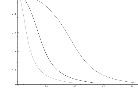
Figure 2: Hubble parameter (in units of $H_{0}$) at times $1/H_{0},2/H_{0},3/H_{0}$

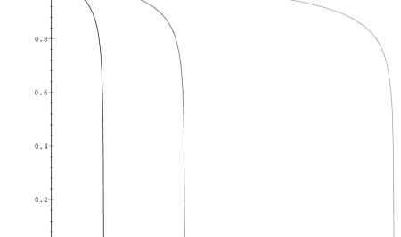
Figure 3: Hubble parameter (in units of $H_{0}$) at times $10/H_{0},11/H_{0},12/H_{0}$

Knowing the evolution of the scale factor allows one to calculate the temperature and energy density from pre-inflationary quantities. This will allow us to determine these quantities at the end of inflation and then use them as initial conditions for the standard cosmology; hopefully giving some observable variations in quantities to test our model.

We shall assume that before inflation there was a uniform radiation energy density $\rho_{0}$ at temperature $T_{c}$, the critical temperature of phase transition. We shall also assume that once the initial transient phase of inflation is complete the radiation density does not appreciably effect the evolution of the scale factor in eq. (39); this is motivated through observing that Universe expansion dilutes $\rho$ whilst not affecting the vacuum energy density. For radiation, $\rho$ scales as $a^{-4}$, whilst the temperature $T$ scales as $1/a$. This yields the following two evolution equations:

$$\mbox{$\rho$}(r,t)=\rho_{0}\left(\frac{a_{0}}{a(r,t)}\right)^{4} = \mbox{$\rho$}_{o}\exp\left(-4tH_{0}(1-f_{\rm mon}(r)^{2})\right),$$ (42a)

$$T(r,t)=T_{c}\frac{a_{0}}{a(r,t)} = T_{c}\exp\left(-tH_{0}(1-f_{\rm mon}(r)^{2})\right).$$ (42b)

As always, the spatial variations must be interpreted with the physical distance $r^{\prime}$.

We shall now estimate the required number of e-folds of inflation. To do this we simply estimate the amount of inflation needed to expand the monopole’s core to a region of our present horizon size. This region is in causal contact with us now, and hence the number of e-folds of inflation must be sufficient (or more) to create a region of this size. If there was less inflation we should have observed some effects from the edge of the inflated core — which are quite severe (see later). We have not seen such effects.

The initial size of the monopole is, from eq. (2.4), $r_{\rm core}=2(g\eta)^{-1}$. The coupling constant $g$ is known to be about $1/50$ and the scale of symmetry breaking $\eta$ is required to be about $10^{18}\rm{GeV}$. Hence,

$$r_{\rm core}\sim\frac{10}{3}\times 10^{-17}{\rm GeV}^{-1}\sim 6\times 10^{-29}{\rm m},$$ (43)

To estimate the final size of the core after inflation, we estimate $H(r)$ to be $H(0)=H_{0}$; this is expected to be correct to within a factor of two or so, and since we shall be dealing in orders of magnitude it should prove to be a good approximation. This yields the final core size to be

$$d(t_{I})=r_{\rm core}\exp\left(\sqrt{\frac{8\pi\lambda\eta^{4}}{3m_{\rm pl}^{2}}}t_{I}\right)=r_{\rm core}\exp(N),$$ (44)

with $N$ the number of e-folds and $t_{I}$ the duration of inflationary expansion. The size of the core $d(t_{I})$ needs to be greater than the size of our presently observable Universe, which can be estimated from the age of our Universe, which is found from the present Hubble constant. A standard and simple calculation gives:

$$d_{\rm universe}\sim\frac{6}{h}\times 10^{25}{\rm m},$$ (45)

where $h\sim 0.6-0.8$. We define $N_{\rm crit}$ to be the minimum number of e-folds required to produce a Universe as large as that presently observed; the actual number of e-folds being expected to be larger than this (though, see sec. (4.9)). Equating $d_{\rm universe}=r_{\rm core}\exp(N_{\rm crit})$, one obtains

$$N_{\rm crit}={\rm ln}(\frac{2}{h}\times 10^{4}),$$ (46)

and substituting above for $h$:

$$N_{\rm crit}=125,$$ (47)

which is pretty much insensitive to the value of $h$. This solves the horizon problem in the usual way, since the core of the monopole is in causal contact before inflation. In addition, the number of e-folds estimated above easily satisfies the bounds on flatness; which requires the number of e-folds to be larger than about sixty.

Estimating the actual number of e-folds of inflation to be about the critical value, $N\sim N_{\rm crit}$, gives us an estimate of how the Hubble parameter, temperature and pre-inflationary radiation density vary with physical distance $r^{\prime}$; this variation being at the point when inflation is ending, the monopole starting to decay, but reheating not yet occurring. Extrapolating figs. (2) and (3) to $125$ e-folds of inflation, one sees that the variation in the Hubble parameter with distance is reasonably uniform upto the horizon, where a sharp falloff (essentially to zero) takes place. Calculation verifies, with there only being a one per cent variation in the Hubble parameter upto distances of $(4/5)d_{\rm universe}$.

The distribution in temperature and pre-inflationary radiation density is even more sharply defined. After $125$ e-folds the distribution is approximately:

$$\rho(r,t_{I}) = \left\{\begin{array}[]{ll}0.5\times 10^{-104}\times\rho_{0}\ \ \ \ r^{\prime}<d_{\rm universe}\\ \rho_{0}\ \ \ \ \ r^{\prime}\geq d_{\rm universe}\end{array}\right.$$ (48c)

$$T(r,t_{I}) = \left\{\begin{array}[]{ll}10^{-26}\times T_{c}\ \ \ \ r^{\prime}<d_{\rm universe}\\ T_{c}\ \ \ \ \ r^{\prime}\geq d_{\rm universe}\end{array}\right.$$ (48f)

This massive dilution of the initial temperature and density of the Universe renders the initial radiation density completely unobservable. These miniscule remnants will be absorbed into the radiation produced from reheating, of which the remnants’ contribution will be insignificant. However, conditions before inflation are still present outside the inflated region. As we can see from the plots the divide is immensely sharp; due to the scale parameter decreasing sharply to unity at the boundary of the monopole’s core.

4.4 The End of Inflation : Decay of the Monopole.

It is difficult to model the decay of the monopole. We have derived eq. (35) showing how the scalar field would decay if all the gauge fields were diluted away by inflation. However, eq. (35) ignores the gravitational back reaction on the scalar field. Hence, this equation is of limited use — only in showing the connection between topology and eternal inflation.

The arguments given in sec. (4.2) indicate how a long lived embedded monopole may occur. Qualitatively, when the monopole decays there is one of two ways it can do it:

• Quickly. The embedded monopole lives in a long-lived stationary state and then all points decay quickly simultaneously. This could happen naturally by rolling, or could also be due to quantum tunnelling processes.

• Slowly. Points on the edge of the core decay before points at the centre, with an appreciable time lag. Should create appreciable large scale inhomogeneities in cosmological parameters.

We shall assume the quick rolling scenario for simplicity. However, it should be noted that large scale homogeneities in the slow decay scenario would be severely decreased by later Universe evolution.

4.5 Reheating

In all models of inflation there is reheating, where the vacuum energy (that does not scale with expansion) is converted into a radiation energy density which is the origin of (virtually) all matter we see today. The duration of reheat determines the temperature (i.e. efficiency) produced. Owing to our model being inhomogeneous, one may expect variations in the local energy density and temperature.

The mechanism of reheating is unchanged for our model; the only difference being that not all points in the Universe are necessarily required to reheat at the same time, or have the same vacuum energy. As usual, we shall neglect spatial gradients, so as to approximate by local standard cosmologies.

We shall use the old mechanism of reheat; not the new more sophisticated one (where one treats properly parametric resonance of the scalar field) [23]. We are motivated into this choice by the comparitive simplicity, and, of course, a proper theory of reheat should consider the theory of parametric resonance. The scalar field decays into coherent oscillations around the bottom of the potential well, then these oscillations decay into radiation. The rate of oscillation decay determines the rate of reheating.

Assuming the dominant decay width of the Higgs is into the most massive particle — namely, the Lepto-quark bosons — the decay width may be estimated to be

$$\Gamma_{\phi}\sim g^{2}m_{\rm LQ}=g^{3}\eta.$$ (49)

Then the decay time of the coherent oscillations, which is the reheat time, is about $\Gamma^{-1}$. To properly estimate this one should compare it to the Hubble expansion time at the end of inflation $H^{-1}$. The ratio of these two quantities gives the number of Hubble expansion times for reheating; which is

$$\frac{\Gamma_{\phi}^{-1}}{H(r,t_{I})^{-1}}\sim\sqrt{\frac{5\pi}{3}}\left(\frac{\eta}{m_{\rm pl}}\right)\frac{\sqrt{\lambda}}{g^{3}}(1-f_{\rm mon}(r)^{2}).$$ (50)

If $\Gamma_{\phi}^{-1}/H(r,t_{I})^{-1}\ll 1$, reheat is practically instantaneous to a temperature

$$T_{\rm RH}\sim\left(\frac{45}{4\pi^{3}g_{*}}\right)^{1/4}(H(r,t_{I})m_{\rm pl})^{1/2}.$$ (51)

For $\Gamma_{\phi}^{-1}/H(r,t_{I})^{-1}\gg 1$, reheat is long compared to the relevant Hubble expansion rate; the Universe then expands as if matter dominated for the time $\Gamma^{-1}$, after which the oscillations are quickly damped — producing a reheat temperature

$$T_{\rm RH}\sim\left(\frac{30}{\pi^{2}g_{*}}\right)^{1/4}(\Gamma_{\phi}m_{\rm pl})^{1/2}.$$ (52)

One should note that this is independent of the Hubble parameter.

Estimating parameters to be $g\sim 1/50$, $\eta/m_{\rm pl}\sim 1/10$, one finds the rate of reheat to be dependent on $\lambda$ only with the two cases:

$$\mbox{$\lambda$}<O(10^{\rm-10}) \Rightarrow \ {\rm FAST\ REHEAT}\ {\rm with}\ T_{\rm RH}\sim\frac{\eta}{2}\lambda^{1/4}(1-f_{\rm mon}(r)^{2})^{1/2}$$ (53a)

$$\mbox{$\lambda$}>O(10^{\rm-10}) \Rightarrow \ {\rm SLOW\ REHEAT}\ {\rm with}\ T_{\rm RH}\sim 4\times 10^{15}{\rm GeV}.$$ (53b)

There are two notes that one should make. Firstly, for a fast reheat there is variation with $r$ (distance from the centre of the core), whereas for slow reheat there is not. Secondly, in this model it is difficult to obtain a low temperature of reheat.

4.6 Evolution of an Inhomogeneous Universe

It is necessary, before the discussion on large scale inhomogeneities after inflation, to discuss how the Universe evolves with a non-uniform energy density. We shall model the evolution of such a Universe by the usual approximation: neglecting spatial gradients and treating as locally FRW.

There are two cases necessary to discuss: radiation dominated or matter dominated. The two cases differ by an equation of state, where the pressure is related to the energy density,

$$P = \frac{1}{3}\rho,\ \ \ \ \ \ \ (RADIATION)$$ (54a)

$$P = 0.\ \ \ \ \ \ \ \ \ \ (MATTER)$$ (54b)

The relevance of the different states being that the evolution of coherent oscillations of the Higgs field during reheating is matter dominated. The evolution of the decay products being radiation dominated.

Supposing the time at the end a previous era of Universe evolution is $t_{0}(r)$, with an energy density (matter or radiation) of

$$\rho(r^{\prime},t_{0})=\rho_{\rm RH}(r^{\prime},t_{0})+\rho_{\rm in}(r^{\prime},t_{0}),$$ (55)

the two terms representing the contributions from energy density from reheating (respectively either a radiation density or a matter density in the form of coherent oscillations), and the initial radiation density of the Universe. The initial radiation density was described in section (4.3) — being approximately zero inside the core, and GUT scale outside.

In modelling the evolution of the Universe we shall ignore the effects of $\rho_{\rm in}$ for the following reason. The initial radiation density has the appearance of a wall; on our side it is approximately zero and on the other side it is of GUT scale. This wall would move towards us at the speed of light. Effects on the scale factor and density are inside the Cauchy surface of such a wall, which coincide with the edge of the wall itself. In essence, since the wall moves at (approximately) the speed of light, no effects can be seen until it hits you. This initial radiation density becomes, however, important at very late times — as we shall discuss in the sec. (4.9).

4.6.1 Radiation Dominated

Neglecting spatial gradients, the evolution equations for the scale factor are locally FRW, with $k=0$,

$$\left(\frac{\dot{a}}{a}\right)^{2} = \frac{8\pi G\rho_{\rm RH}(r,t_{0})}{3}\left(\frac{a(r^{\prime},t_{0})}{a(r,t)}\right)^{4}$$ (56a)

$$2\frac{\ddot{a}}{a}+\left(\frac{\dot{a}}{a}\right)^{2} = \frac{8\pi G\rho_{\rm RH}(r,t_{0})}{3}\left(\frac{a(r^{\prime},t_{0})}{a(r,t)}\right)^{4}.$$ (56b)

Normalising $a(r^{\prime},t_{0})=1$, we obtain the following solution

$$a(r^{\prime},t)=\left(2H(r,t_{\rm RH})(t-t_{0})+1\right)^{1/2},$$ (57)

with the consistency relation that the Universe is locally flat (i.e. we may neglect spatial curvature) when that area of Universe changes its equation of state:

$$H(r^{\prime},t_{0})^{2}=\frac{8\pi G}{3}\rho(r,t_{0}),$$ (58)

which is essentially conservation of energy.

Thus we may calculate the evolution of the Hubble constant and energy density to be, inside the core of the monopole:

$$H(r^{\prime},t)=\frac{\dot{a}}{a} = \frac{H(r,t_{0})}{1+2H(r,t_{0})(t-t_{0})},$$ (59a)

$$\rho(r,t) = \frac{\rho(r,t_{0})}{\left(1+2H(r,t_{0})(t-t_{0})\right)^{2}}.$$ (59b)

It is important to note that at late times the initial distribution of the Hubble parameter is homogenised. If one considers $(t-t_{0})\ll 1/H$ the usual expression for the Hubble parameter is obtained, i.e. $H(r^{\prime},t)\sim 1/(2(t-t_{0}))$.

4.6.2 Matter Dominated

The analysis follows through exactly as for the last section: we approximate by locally FRW Universes, neglecting spatial gradients. We also assume the Universe is still spatially flat ($k=0$), which is to be expected after $120$ e-folds of inflation.

Initially the Hubble constant is $H(r,t_{0})$ and the matter density is $\rho(r,t_{0})$. The Universe is supposed to be dust filled, with zero pressure. Thus, the local FRW equations are:

$$\left(\frac{\dot{a}}{a}\right)^{2} = \frac{8\pi G\rho_{\rm RH}(r,t_{0})}{3}\left(\frac{a(r^{\prime},t_{0})}{a(r,t)}\right)^{3}$$ (60a)

$$2\frac{\ddot{a}}{a}+\left(\frac{\dot{a}}{a}\right)^{2} = 0.$$ (60b)

Normalising $a(r^{\prime},t_{0})=1$, we obtain the following solution

$$a(r^{\prime},t)=\left(\frac{3}{2}H(r,t_{0})(t-t_{0})+1\right)^{2/3},$$ (61)

with the consistency relation that the Universe is locally flat when that area of Universe changes its equation of state:

$$H(r^{\prime},t_{0})^{2}=\frac{8\pi G}{3}\rho(r,t_{0}),$$ (62)

Then the evolution of the matter density and the Hubble constant may be calculated to be:

$$H(r^{\prime},t)=\frac{\dot{a}}{a} = \frac{H(r,t_{0})}{1+(3/2)H(r,t_{0})(t-t_{0})},$$ (63a)

$$\rho(r,t) = \frac{\rho(r,t_{0})}{(1+(3/2)H(r,t_{0})(t-t_{0}))^{2}}.$$ (63b)

As above, at late times the initial distribution of the Hubble parameter is homogenised. If one considers $(t-t_{0})\ll 1/H$ the usual expression for the Hubble parameter is obtained, i.e. $H(r^{\prime},t)\sim 2/(3(t-t_{0}))$.

4.7 From de-Sitter to Radiation Dominated Evolution

There are essentially two processes, which may be quick or slow, that determine large scale inhomogeneities in the distributions of the Hubble constant, energy density and temperature after inflation. Firstly, the decay of the monopole: which may be quick or slow. Secondly, the duration of reheat (which depends upon the parameter $\lambda$); in slow reheat the universe evolves with matter dominating coherent oscillations of the Higgs field before the radiation dominated era.

Hence there are a total of four different situations. For simplicity, we shall assume the monopole decays quickly (i.e all points simultaneously) and deal with the two cases of quick and slow reheat.

If the monopole were to decay slowly, any non-simultaneity of decay would be transmitted into inhomogeneities of the cosmological parameters. We do not discuss such a case.

4.7.1 Quick Monopole Decay; Fast Reheat

This is the simplest case and is valid for $\lambda<O(10^{-10})$. It is possible to implement this in both SUSY and NON-SUSY field theories. The cosmology goes like:

• Quick monopole decay, freezing in variations of the Hubble parameter, energy density and temperature.

• Universe reheats quickly from a rapid decay of coherent Higgs oscillations into radiation, reheating the Universe.

We now expand upon this sketch, putting values to the variables. To obtain a Universe at least as large as observed today one needs at least $125$ e-folds of inflation (see eqs. (44) - (47)). For simplicity, assume that this is the exact amount of e-folding performed. Also assume that the quartic Higgs coupling $\lambda$ is in the range $10^{-9}-1$, taking these outer two values for computing. In addition we shall take $\eta/m_{\rm pl}\sim 1/10$.

Then at the end of inflation the Hubble constant is (from eq. (41)):

$$\frac{H(r,t_{\rm inf})}{1-f_{\rm mon}(r)^{2}}=\frac{3\lambda^{1/4}\eta}{10}{\rm GeV}=5\times 10^{39}-5\times 10^{41}{\rm ms^{-1}m^{-1}}.$$ (64)

The distribution is very sharp because the physical distance scale scales sharply, being related to $r$ by $r^{\prime}(r,t_{\rm inf})=\int_{0}^{r}\exp\left(125(1-f_{\rm mon}(x)^{2})\right)dx$.

The scaling of the pre inflationary radiation density is even more severe: having a miniscule temperature of about $10^{-26}\times T_{c}{\rm GeV}$ inside the inflated region and about $T_{c}$ outside.

The monopole decays quickly, freezing in the above variation of the Hubble parameter. At all points in space the Higgs field falls down into its potential well, oscillating around the bottom. These oscillations are coherent and decay quickly (for the parameters considered here) to a non-uniform temperature:

$$T_{\rm RH}\sim\left\{\begin{array}[]{ll}\frac{\eta}{2}\lambda^{1/4}(1-f_{\rm mon}(r)^{2})^{1/2}\ \ \ \ r^{\prime}<d_{\rm universe}\\ T_{c}\ \ \ \ \ r^{\prime}\geq d_{\rm universe}\end{array}\right.$$ (65)

and by eq. (58) we determine the density to be:

$$\rho(r,t_{\rm inf})=\left\{\begin{array}[]{ll}\frac{3H_{0}^{1/2}}{8\pi G}(1-f_{\rm mon}(r)^{2})^{1/2},\ \ \ \ r^{\prime}<d_{\rm universe}\\ \rho_{c}\ \ \ \ \ r^{\prime}\geq d_{\rm universe}\end{array}\right.$$ (66)

which scales the same as temperature.

The Universe then evolves as radiation dominated, according to eq. (4.6.1).

4.7.2 Quick Monopole Decay; Slow Reheat

This case is valid for $\lambda<O(10^{-10})$.

• Quick monopole decay, freezing in variations of the Hubble parameter, energy density and temperature.

• A long period of reheat, where the Universe evolves with coherent Higgs oscillations defining the equation of state, which is matter dominated. The matter dominated evolution homogenises the large scale variations in cosmological parameters.

• A rapid decay of coherent Higgs oscillations into radiation, reheating the Universe.

We complement this sketch with a more detailed examination of the transition.

The treatment follows as above for the decay of the monopole and hence for the initial distribution of the Hubble parameter. However, now the coherent Higgs oscillation take a long time to decay and the Universe evolves as matter dominated for a time $t\sim\Gamma_{\phi}^{-1}=(g^{3}\eta)^{-1}$. Using eq. (62), one determines the Hubble parameter to vary as:

$$H(r,t_{\rm RH}) = \frac{H_{0}(1-f_{\rm mon}(r)^{2})}{1+\frac{3H_{0}}{g^{3}\eta}(1-f_{\rm mon}(r)^{2})},$$ (67)

$${\rm with}\ \ \ \ \frac{3H_{0}}{g^{3}\eta} \sim 5\times 10^{5}\sqrt{\lambda}.$$ (68)

Hence as long as $\lambda>O(10^{-10})$, the effects of the Higgs oscillations are important on the variation of the Hubble parameter. For $\lambda\gg O(10^{-10})$ these effects homogenise the Hubble parameter to the value

$$H(r,t_{\rm RH})\sim\frac{2}{3}g^{3}\eta\sim 5\times 10^{12}{\rm GeV}.$$ (69)

Then the decay of coherent Higgs oscillations is quick, leading to a reheat temperature

$$T_{\rm RH}\sim\frac{2}{5}(g^{3}\eta m_{\rm pl})^{1/2}\sim 5\times 10^{15}{\rm GeV}.$$ (70)

4.8 Constraints from Gravitational Radiation

It is well known that Planck scale inflationary models produces copious amounts of gravitational radiation. This gravitational radiation gives a contribution to the cosmic microwave background [24]. Thus COBE anisotropy measurements constrain such inflationary models.

The model of inflation presented in this paper is locally similar to standard models of vacuum dominated inflationary models; though with the vacuum characterised by the energy density

$$\epsilon=\lambda\eta^{4}(1-f_{\rm mon}(r)^{2})^{2}.$$ (71)

Hence, from [24] the contribution to the quadrupole moment of the cosmic microwave background is

$$\left(\frac{\Delta T}{T}\right)_{\rm quad}=2.4\frac{\lambda\eta^{4}}{m_{\rm pl}^{4}}(1-f_{\rm mon}(r)^{2})^{2}.$$ (72)

COBE gives the observed quadrupole anisotropy to be $(\Delta T/T)_{\rm quad}\sim 7\times 10^{-6}$. Estimating $(\eta/m_{\rm pl})\sim 0.1$ yields the following constraint on $\lambda$

$$\lambda<3\times 10^{-2}.$$ (73)

It should be noted that there may be other contributions to the quadrupole anisotropy that may further constrain $\lambda$.

4.9 The Universe at Very Late Times

Examining eq. (3), one sees that the divide between the inflated region of space and the uninflated GUT scale regions is extremely sharp; being completely due to the scaling of the distance scale, eq. (40). One could also interpret this as a massive time dilation as one passes from present day physics to GUT-scale physics across this divide.

The upshot of this is that this scenario for inflation predicts a region of space akin to our own, but surrounded by a wall of GUT scale energy. Across the wall there is a massive pressure difference caused by the large density (and temperature) variation. Such a wall would move into the inflated region at practically the speed of light.

We have shown previously (eqs. (44) - (47)) that in order to create a region of space at the end of inflation large enough to contain our presently observable Universe (i.e. the wall has not hit us) the number of e-folds of inflation has to be greater than $N_{\rm crit}=125$. The question is, therefore, given that at least $125$ e-folds of inflation has taken place, how many more e-folds can we expect — i.e. how much longer do we have before this wall of energy hits us?

Recall that the number of e-folds of inflation determines the size of the inflated region by (we are talking about the diameter, assuming the region to be spherical)

$$d_{\rm universe}=d_{\rm core}e^{N},\ {\rm where}\ N=H_{0}t_{\rm decay},$$ (74)

where the core radius $d_{\rm core}=2(g\eta)^{-1}$, $H_{0}$ is the Hubble parameter of eq. (39) and the decay time of the monopole is probabilistically distributed as (from eq. (36))

$$P(t_{\rm decay}>t)=e^{-\frac{t}{\alpha}}.$$ (75)

The expected (mean) time of decay is $\bar{t}=\alpha$. For small times $\alpha\sim\eta^{-1}$ (determining whether inflation initiates). After inflation initiates, the characteristic time scale is the Hubble time $H_{0}^{-1}$. Thus for large times we estimate $\alpha\sim H_{0}^{-1}$ and the above distribution is approximately Poisson, as long as we are conditional on the monopole not decaying quickly.

Given the number of e-folds of inflation is greater than $125$, the Poisson nature of the probability distribution at large times gives the conditional probability for the number of e-folds:

$$P({\rm e-folds}>N\ |\ N>N_{\rm crit})=\exp\left(\frac{N-N_{\rm crit}}{H_{0}\alpha}\right).$$ (76)

This yields the expected number of e-folds of inflation conditional on $N>N_{\rm crit}$ to be

$$\bar{N}=N_{\rm crit}+1.$$ (77)

Hence if one estimates the age of our Universe (the time since inflation finished) to be about $10-15$Gyr, from which the size of our observable universe is about $10^{26}$m. Then the actual size of inflationary universe created in this model of inflation is probabilistically distributed with a mean of $e$ times this. Before estimating the amount of time left, one should remember that we are not necessarily at the ‘center’ of the Universe, but somewhere randomly distributed in the Universe that has not seen the wall of energy coming towards us — this gives a factor of half from our expected time. Hence we can realistically expect about $(e-1)/2\times 10-15$Gyrs, i.e. about $8-13$Gyrs left .

5 Conclusions

By nature, the work in this paper is open ended. Hence, in this section we shall briefly discuss some directions in which the work could be extended. We shall briefly discuss the consequences of non-spherically symmetric decay; realisation with other unstable defects; and the cause and observation of large scale inhomogeneities from such scenarios.

However, firstly we shall give a brief summary of the features of non-topological inflation as presented in this paper.

5.1 Non-topological Inflation

We consider a Yang-Mills field theory that realistically describes a GUT. Our theory must have monopole solutions

$$\mbox{$\Phi$}(r,\th) = f_{\rm mon}(r)\underline{\hat{r}},$$

$$A(r,\th) = \frac{g_{\rm mon}(r)}{qr}\epsilon_{\mu ab}T_{b},$$

where $q$ is the order of the coupling constants and $f_{\rm mon}(r)$ and $g_{\rm mon}(r)$ are the profile functions of the monopole. Monopole solutions may be either stable or unstable.

• Coupling the monopole solution to gravity yields inflation provided

  $$\left(\frac{\eta}{m_{\rm pl}}\right)^{2}>\frac{1}{4\pi}.$$

  Additionally $\lambda$ is constrained so that

  $$\frac{1}{2}\lambda\left(\frac{\eta}{m_{\rm pl}}\right)^{2}<1,$$

  otherwise the monopole becomes a black hole.

• The inflating monopole solution has a Hubble parameter distribution of

  $$H(r,t)=\frac{\dot{a}}{a}=H_{0}\left(1-f_{\rm mon}(r)^{2}\right),$$

  $${\rm where}\ \ H_{0}=\sqrt{\frac{8\pi\lambda\eta^{4}}{3m_{\rm pl}^{2}}}.$$

  and the physical coordinate $r^{\prime}$ is related to $r$ by the scaling relation $r^{\prime}(r,t)=\int_{x=0}^{r}\frac{a(x,t)}{a_{0}}{\rm d}x$, with $a$ the scale factor which, during inflation, is of the form $a(r,t)=a_{0}\exp(H_{0}t(1-f_{\rm mon}(r)^{2}))$.

• Topologically stable monopoles inflate eternally: difficult to reconcile with the present state of the Universe. Unstable monopoles decay probabilistically: stipulate that we lived in such a monopole that (randomly) lived long enough for us to exist.

• For the Universe to be as large as we see today (the diameter of the Universe $d_{\rm universe}\sim 10^{26}m$) one requires the decay time $t_{\rm decay}>125H_{0}^{-1}$. After such time the distribution of initial density and temperature is:

  $$\rho(r,t_{I}) = \left\{\begin{array}[]{ll}0.5\times 10^{-104}\times\rho_{0}\ \ \ \ r^{\prime}<d_{\rm universe}\\ \rho_{0}\ \ \ \ \ r^{\prime}\geq d_{\rm universe}\end{array}\right.$$ (80)

  $$T(r,t_{I}) = \left\{\begin{array}[]{ll}10^{-26}\times T_{c}\ \ \ \ r^{\prime}<d_{\rm universe}\\ T_{c}\ \ \ \ \ r^{\prime}\geq d_{\rm universe}\end{array}\right.$$ (83)

  and the form of the Hubble parameter is also very sharp. Here $r^{\prime}$ is the physical radial coordinate.

• The monopole then decays. Resulting reheat (from coherent oscillations of the scalar field about the bottom of the potential) slow if $\lambda>O(10^{-10})$ and fast otherwise. Temperature of reheat distributed as:

  $${\rm FAST\ REHEAT}\ {\rm with} \ T\sim\left\{\begin{array}[]{ll}\frac{\eta}{2}\lambda^{1/4}(1-f_{\rm mon}(r)^{2})^{1/2}\ \ \ \ r^{\prime}<d_{\rm universe}\\ T_{c}\ \ \ \ \ r^{\prime}\geq d_{\rm universe}\end{array}\right.$$ (86)

  $${\rm SLOW\ REHEAT}\ {\rm with} \ T\sim\left\{\begin{array}[]{ll}4\times 10^{15}{\rm GeV}\ \ \ \ r^{\prime}<d_{\rm universe}\\ T_{c}\ \ \ \ \ r^{\prime}\geq d_{\rm universe}\end{array}\right.$$ (89)

  where $r$ is related to the physical coordinate $r^{\prime}$ by the scaling relation above.

• After reheating the Hubble parameter is distributed as:

  $${\rm FAST\ REHEAT}\ {\rm with} \ H(r,t_{\rm RH})\sim\left\{\begin{array}[]{ll}\frac{3\lambda^{1/4}\eta}{10}(1-f_{\rm mon}(r)^{2})\ \ r^{\prime}<d_{\rm universe}\\ 0\ \ \ \ \ r^{\prime}\geq d_{\rm universe}\end{array}\right.$$ (92)

  $${\rm SLOW\ REHEAT}\ {\rm with} \ H(r,t_{\rm RH})\sim\left\{\begin{array}[]{ll}\frac{2}{3}q^{3}\eta\ \ \ \ r^{\prime}<d_{\rm universe}\\ 0\ \ \ \ \ r^{\prime}\geq d_{\rm universe}\end{array}\right.$$ (95)

  where, as usual, one uses the scaled distance.

• For inflationary gravitational radiation to be less than present bounds, one requires:

  $$\lambda<3\times 10^{-2}.$$

• The divide between inflationary and non-inflationary region is very sharp and moves into the inflationary region at (practically) the speed of light. Given the Universe is at least as large as we see, the conditional expectation value for the amount of time left before the wall reaches us is around $8-14$Gyrs.

5.2 Non-Spherically Symmetric Decay

In the above treatment of inflation, we have always assumed that our monopole decays through a spherically symmetric mode. Hence, the distribution of cosmological parameters has also spherical symmetry around the centre of the monopole.

However, there are other decay modes as well as the spherically symmetric one. Higher decay modes correspond to higher spherical harmonics, and although they correspond to higher energies, the route by which the monopole decays depends upon the initial conditions of the monopole — which are random. The spherical mode we have been using corresponds to the lowest energy mode $Y_{00}(\th,\phi)$, higher energy decay modes correspond to $Y_{lm}(\th,\phi)$ harmonics. The lowest harmonic that is non-spherically symmetric is the $Y_{1m}(\th,\phi)$, with $m=-1,0,1$, and gives a dipolar decay — resulting in an ellipsoidal inflated region.

In general one may expect that the decay is the linear superposition of several decay modes.

5.3 Realisation with other Defects

Although the treatment, so far, has only been concerned with embedded monopoles, it does seem likely that it may also be realisable with other defects — such as embedded vortices or embedded domain walls. The important criterion for inflation is longevity of the defect, which we argue can be due to the defect having a corresponding saddle point in configuration space. Embedded vortices and embedded domain walls also have saddle points in configuration space, and are thus also inflationary candidates.

Each type of defect gives a different symmetry of cosmological parameters: an embedded vortex should give rise to cylindrical symmetry (with superimposed harmonic decay modes) and an embedded domain wall would give rise to cosmological parameters with reflection symmetry.

5.4 Possible Observable Consequences

From our results on the distribution of cosmological parameters after inflation, one can see that the parameters (temperature, density, Hubble parameter) decrease towards the edge of the inflated region. Since the decrease is so small and is so close to the edge of the inflated region such inhomogeneities could only be manifest in quantities that originated a very long time ago, just reaching us now. Possible candidates are either a decrease in the Cosmic Microwave Background temperature (unlikely to be detectable because of uncertainty in the Hubble constant now); or, more likely, the Cosmic Neutrino Background temperature (which decouples at about $10^{-9}$ seconds). Since the Cosmic Neutrino background has never been observed, this is, of course, only a speculation.

It should be noted that a non-spherically symmetric Universe (either from higher monopole decay modes or by using other defects) would give a non-spherically symmetric (i.e. non-uniform) contribution to the Cosmic microwave and Neutrino backgrounds.

Acknowledgements.

This work is supported in part by PPARC. We acknowledge EPSRC for research studentships. We wish to thank A.C. Davis and M. Trodden for interesting discussions related to this work.

Appendix: The Non-existence of Sphalerons in Flipped-$SU(5)$

For the later parts of this paper it is important to know what monopole-type configurations are solutions to flipped-$SU(5)$. In [8] the motivation for studying V-strings in flipped-$SU(5)$ came from an analogy in structure between flipped-$SU(5)$ and the Weinberg-Salam model. Carrying the analogy further leads to a consideration of the existence of Sphaleron configurations. We shall now show that, rather surprisingly, such a configuration is not a solution to flipped-$SU(5)$.

If a Sphaleron configuration was a solution to flipped-$SU(5)$ then an embedded subtheory could be constructed which contains it. The form of the embedded subtheory has to be the same as the Weinberg-Salam model. Namely $G_{{\rm emb}}=SU(2)\times U(1)$, with $H_{{\rm emb}}=H\cap G_{{\rm emb}}=U^{\prime}(1)$, where $U^{\prime}(1)$ is generated by a linear combination of a generator of $U(1)$ and $SU(2)$. A little thought shows that $G_{{\rm emb}}\subset SU(5)\times\widetilde{U(1)}$ in the following way:

$$SU(5) \times \widetilde{U(1)}$$

$$\cup\ \ \ \|$$ (96)

$$SU(2) \times U(1)$$

with $H_{{\rm emb}}=U(1)_{Y}$. For the breaking $G_{{\rm emb}}\rightarrow H_{{\rm emb}}$ to properly mirror that of the Weinberg-Salam model the generators of the $SU(2)$-algebra $\{T,T^{\prime},[T,T^{\prime}]\}$ must be such that

$$T,T^{\prime}\in\underline{m}_{2},\ \ \ {\rm with}\ \ \ [T,T^{\prime}]=T^{15}.$$ (97)

It is this condition that cannot be satisfied.

As $\{T,T^{\prime},T^{15}\}$ generate an $SU(2)$-algebra, the following relation holds:

$$[T,[T,T^{15}]]=T^{15}.$$ (98)

Taking $T$ to be defined as in eq. (11) yields the following relations:

$$\underline{A}\underline{A}^{\dagger} = \frac{1}{5}{\bf 1}_{3},$$ (99a)

$$\underline{A}^{\dagger}\underline{A} = -\frac{3}{10}{\bf 1}_{2},$$ (99b)

which gives

$$\underline{v}_{i}^{\dagger}\underline{v}_{j}=\frac{1}{5}\delta_{ij}.$$ (100)

Since $\underline{v}_{i}$ is a two-component complex vector, eq. (100) says that we must find three orthogonal vectors in a two-dimensional vector space. This is impossible.

References

- [1] A. H. Guth, Phys. Rev. D. 23 347 (1981).
- [2] A. Linde, Phys. Lett. B372, 208 (1994); A. Vilenkin, Phys. Rev. lett. 72, 3137 (1994).
- [3] A. D. Linde and D. A. Linde, Phys. Rev. D. 50 2456 (1994).
- [4] N. Sakai, H-A. Shinkai, T. Tachizawa, and K. Maeda, Preprint WU-AP-49-95 gr-qc/9506068 (1995). (To be published in phys. rev. D)
- [5] M. Barriola, T. Vachaspati and M. Bucher, Phys. Rev. D. 50 2819 (1994).
- [6] G. t’Hooft, Nucl. Phys. B79, 276 (1976); A. M. Polyakov, JETP Lett. 20, 194 (1974), Nucl. Phys. B120, 429 (1977).
- [7] N. F. Lepora and A. C. Davis, DAMTP/95-06, hep-ph/9507457 (1995). (To be published in phys. rev. D)
- [8] A. C. Davis and N. F. Lepora, Phys. Rev. D. (1995)
- [9] E. W. Kolb and M. S. Turner, The Early Universe, Frontiers in Physics Lecture Note Series, Addison Wesley (1990).
- [10] P. Langacker and N. Polonsky, Phys. Rev. D 47, 4028 (1993).
- [11] J. L. Lopez, D. V. Nanopoulos and K. Yuan, Nucl. Phys. B399, 654 (1993).
- [12] S. Barr, Phys. Lett. 112B, 218 (1982).
- [13] N. F. Lepora and A. C. Davis, DAMTP/95-44, hep-ph/9507466 (1995). (To be published in phys. rev. D)
- [14] N. Manton, Phys. Rev. D 28 2019 (1983); F. Klinkhamer and N. Manton, Phys. Rev. D 39 2212 (1984).
- [15] M. K. Prasad and C. M. Sommerfield, Phys. Rev. Lett. 35 760 (1975).
- [16] T. W. Kirkman and C. K. Zachos, Phys. Rev. D 24 999 (1981).
- [17] I. Antoniadis, J. Ellis, R. Lacaze, and D. V. Nanopoulos, Phys. Lett. B368, 188 (1991); S. Kalara, J. L. Lopez, and D. V. Nanopoulos, ibid. 269, 84 (1991).
- [18] I. Antoniadis, J. Ellis, J. Hagelin, and D. V. Nanopoulos, Phys. Lett. B194, 231 (1987); I. Antoniadis, J. Ellis, J. Hagelin, and D. V. Nanopoulos, Phys. Lett. B231, 65 (1989).
- [19] J. Lopez, D. Nanopoulos, and A. Zichichi, Phys. Rev. D 49 343 (1994).
- [20] D. A. Kirschnits and A. D. Linde, Ann. Phys. 101 (1976); A. D. Linde, Phys. Lett. 70B, 306 (1977).
- [21] P.J. Steinhardt and M.S. Turner, Phys. Rev. D 29, 2162 (1984).
- [22] T. W. Kibble, J. Phys A9, 1387 (1976).
- [23] L. Kofman, A. Linde, and A. A. Starobinskii, Phys. Rev. Lett. 73, 3195 (1994).
- [24] V. Rubakov, M. Sazhin, and A. Veryaskin, Phys. Lett. B115, 189 (1982).