SLAC–PUB–7106

hep-ph/9601359

January, 1996

CALCULATING SCATTERING AMPLITUDES EFFICIENTLY^⋆

LANCE DIXON

Stanford Linear Accelerator Center

Stanford University, Stanford, CA 94309

ABSTRACT

We review techniques for more efficient computation of perturbative scattering amplitudes in gauge theory, in particular tree and one-loop multi-parton amplitudes in QCD. We emphasize the advantages of (1) using color and helicity information to decompose amplitudes into smaller gauge-invariant pieces, and (2) exploiting the analytic properties of these pieces, namely their cuts and poles. Other useful tools include recursion relations, special gauges and supersymmetric rearrangements.

Invited lectures presented at the Theoretical Advanced Study Institute

in Elementary Particle Physics (TASI 95): QCD and Beyond

Boulder, CO, June 4-30, 1995

  ^⋆Research supported by the US Department of Energy under grant DE-AC03-76SF00515.

1 Motivation

Feynman rules for covariant perturbation theory have been around for almost fifty years, and their adaptation to nonabelian gauge theories has been fully developed for almost twenty-five years. Surely by now every significant standard model scattering process ought to have been calculated to the experimentally-required accuracy. In fact, this is far from the case, especially for QCD, which is the focus of this school and of these lectures. Many QCD cross-sections have been calculated only to leading order (LO) in the strong coupling constant $\alpha_{s}$, corresponding to the square of the tree-level amplitude. Such calculations have very large uncertainties — often a factor of two — which can only be reduced to reasonable levels, say 10% or so, by including higher-order corrections in $\alpha_{s}$.

Currently, no quantities have been computed beyond next-to-next-to-leading-order (NNLO) in $\alpha_{s}$, and the only quantities known at NNLO are totally inclusive quantities such as the total cross-section for $e^{+}e^{-}$ annihilation into hadrons, and various sum rules in deep inelastic scattering. Many more processes have been calculated at next-to-leading-order (NLO), but at present results are still limited to where the basic process has four external legs, such as a virtual photon or $Z$ decaying to three jets, or production of a pair of jets (or a weak boson plus a jet) in hadronic collisions via $q{\bar{q}}\to gg$ ($q{\bar{q}}\to Wg$), etc.

This is not to say that processes with more external legs are not interesting; they are of much interest, both for testing QCD in different settings and as backgrounds to new physics processes. For example, $\alpha_{s}$ could be measured at the largest possible momentum transfers using the ratio of three-jet events to two-jet events at hadron colliders, if only the three-jet process were known at NLO. As another example, QCD is a major background to top quark production in $p\bar{p}$ collisions. If both $t$’s decay hadronically ($t\to Wb\to q{\bar{q}}^{\prime}b$), the background is from six jet production. Despite the fact that the QCD process starts off at $\alpha_{s}^{6}$, it completely swamps the top signal. If one of the two top quarks decays leptonically ($t\to Wb\to\bar{\ell}\nu_{\ell}b$), then QCD production of a $W$ plus three or four jets forms the primary background. This background prevented discovery of the top quark at the Tevatron in this channel, until the advent of $b$ tagging.$\!{}^{{\bf?}}$ Although the NLO corrections to three-jet production are within sight, we are still far from being able to compute the top quark backrounds at NLO accuracy; on the other hand, it’s good to have long range goals.

These lectures are about amplitudes rather than cross-sections. The goal of the lectures is to introduce you to efficient techniques for computing tree and one-loop amplitudes in QCD, which serve as the input to LO and NLO cross-section calculations. (The same techniques can be applied to many non-QCD multi-leg processes as well.) Zoltan Kunszt will then describe in detail how to combine amplitudes into cross-sections.$\!{}^{{\bf?}}$

Efficient techniques for computing tree amplitudes have been available for several years, and an excellent review exists.$\!{}^{{\bf?}}$ One-loop calculations are considerably more involved — they form an “analytical bottleneck” to obtaining new NLO results — and benefit from additional techniques. In principle it is straightforward to compute both tree and loop amplitudes by drawing all Feynman diagrams and evaluating them, using standard reduction techniques for the loop integrals that are encountered. In practice this method becomes extremely inefficient and cumbersome as the number of external legs grows, because there are:

1. too many diagrams — many diagrams are related by gauge invariance.

2. too many terms in each diagram — nonabelian gauge boson self-interactions are complicated.

3. too many kinematic variables — allowing the construction of arbitrarily complicated expressions.

Consequently, intermediate expressions tend to be vastly more complicated than the final results, when the latter are represented in an appropriate way.

In these lectures we will stress the advantages of (1) using color and helicity information to decompose amplitudes into smaller (and simpler) gauge-invariant pieces, and (2) exploiting the analytic properties of these pieces, namely their cuts and poles. In this way one can tame the size of intermediate expressions as much as possible on the way to the final answer. There are many useful technical steps and tricks along the way, but I believe the overall organizational philosophy is just as important. A number of the techniques can be motivated by how calculations are organized in string theory.$\!{}^{{\bf?},{\bf?}}$ I will not attempt to describe string theory here, but I will mention some places where it provides a useful heuristic guide.

The approach advocated here is quite useful for multi-parton scattering amplitudes. For more inclusive processes — for example the $e^{+}e^{-}\to$ hadrons total cross-section — where the number of kinematic variables is smaller, and the real and virtual contributions are on a more equal footing, the computational issues are completely different, and the philosophy of splitting the problem up into many pieces may actually be counterproductive.

2 Total quantum-number management (TQM)

The organizational framework mentioned above uses all the quantum-numbers of the external states (colors and helicity) to decompose amplitudes into simpler pieces; thus we might dub it “Total Quantum-number Management”. TQM suggests that we:

$\bullet$ Keep track of all possible information about external particles — namely, helicity and color information.

$\bullet$ Keep track of quantum phases by computing the transition amplitude rather than the cross-section.

$\bullet$ Use the helicity/color information to decompose the amplitude into simpler, gauge-invariant pieces, called sub-amplitudes or partial amplitudes.

$\bullet$ In many cases we may also introduce still simpler auxiliary objects, called primitive amplitudes, out of which the partial amplitudes are built.

$\bullet$ Exploit the “effective” supersymmetry of QCD tree amplitudes, and use supersymmetry at loop-level to help manage the spins of particles propagating around the loop.

$\bullet$ Square amplitudes to get probabilities, and sum over helicities and colors to obtain unpolarized cross-sections, only at the very end of the calculation.

Carrying out the last step explicitly would generate a large analytic expression; however, at this stage one would typically make the transition to numerical evaluation, in order to combine the virtual and real corrections. The use of TQM is hardly new, particularly in tree-level applications $\!{}^{{\bf?}}$ — but it becomes especially useful at loop level.

2.1 Color management

First we describe the color decomposition of amplitudes,$\!{}^{{\bf?},{\bf?}}$ and review some diagrammatic techniques $\!{}^{{\bf?}}$ for efficiently carrying out the necessary group theory. The gauge group for QCD is $SU(3)$, but there is no harm in generalizing it to $SU(N_{c})$; indeed this makes some of the group theory structure more apparent. Gluons carry an adjoint color index $a=1,2,\ldots,N_{c}^{2}-1$, while quarks and antiquarks carry an $N_{c}$ or $\overline{N}_{c}$ index, $i,{\bar{\jmath}}=1,\ldots,N_{c}$. The generators of $SU(N_{c})$ in the fundamental representation are traceless hermitian $N_{c}\times N_{c}$ matrices, $(T^{a})_{i}^{~{}{\bar{\jmath}}}$. We normalize them according to $\mathop{\rm Tr}\nolimits(T^{a}T^{b})=\delta^{ab}$ in order to avoid a proliferation of $\sqrt{2}$’s in partial amplitudes. (Instead the $\sqrt{2}$’s appear in intermediate steps such as the color-ordered Feynman rules in Fig. 5.)

The color factor for a generic Feynman diagram in QCD contains a factor of $(T^{a})_{i}^{~{}{\bar{\jmath}}}$ for each gluon-quark-quark vertex, a group theory structure constant $f^{abc}$ — defined by $[T^{a},T^{b}]\ =\ i\sqrt{2}\,f^{abc}\,T^{c}$ — for each pure gluon three-vertex, and contracted pairs of structure constants $f^{abe}f^{cde}$ for each pure gluon four-vertex. The gluon and quark propagators contract many of the indices together with $\delta_{ab}$, $\delta^{~{}{\bar{\jmath}}}_{i}$ factors. We want to first identify all the different types of color factors (or “color structures”) that can appear in a given amplitude, and then find rules for constructing the kinematic coefficients of each color structure, which are called sub-amplitudes or partial amplitudes.

The general color structure of the amplitudes can be exposed if we first eliminate the structure constants $f^{abc}$ in favor of the $T^{a}$’s, using

$$f^{abc}\ =\ -{i\over\sqrt{2}}\Bigl{(}\mathop{\rm Tr}\nolimits\bigl{(}T^{a}T^{b}T^{c}\bigr{)}-\mathop{\rm Tr}\nolimits\bigl{(}T^{a}T^{c}T^{b}\bigr{)}\Bigr{)},$$ (1)

which follows from the definition of the structure constants. At this stage we have a large number of traces, many sharing $T^{a}$’s with contracted indices, of the form $\mathop{\rm Tr}\nolimits\bigl{(}\ldots T^{a}\ldots\bigr{)}\,\mathop{\rm Tr}\nolimits\bigl{(}\ldots T^{a}\ldots\bigr{)}\,\ldots\,\mathop{\rm Tr}\nolimits\bigl{(}\ldots)$. If external quarks are present, then in addition to the traces there will be some strings of $T^{a}$’s terminated by fundamental indices, of the form $(T^{a_{1}}\ldots T^{a_{m}})_{i_{2}}^{~{}{\bar{\imath}}_{1}}$. To reduce the number of traces and strings we “Fierz rearrange” the contracted $T^{a}$’s, using

$$(T^{a})_{i_{1}}^{~{}{\bar{\jmath}}_{1}}\,(T^{a})_{i_{2}}^{~{}{\bar{\jmath}}_{2}}\ =\ \delta_{i_{1}}^{~{}{\bar{\jmath}}_{2}}\delta_{i_{2}}^{~{}{\bar{\jmath}}_{1}}-{1\over N_{c}}\,\delta_{i_{1}}^{~{}{\bar{\jmath}}_{1}}\delta_{i_{2}}^{~{}{\bar{\jmath}}_{2}}\,,$$ (2)

where the sum over $a$ is implicit.

Equation 2 is just the statement that the $SU(N_{c})$ generators $T^{a}$ form the complete set of traceless hermitian $N_{c}\times N_{c}$ matrices. The $-1/N_{c}$ term implements the tracelessness condition. (To see this, contract both sides of Eq. 2 with $\delta^{~{}i_{1}}_{{\bar{\jmath}}_{1}}$.) It is often convenient to consider also $U(N_{c})\ =\ SU(N_{c})\times U(1)$ gauge theory. The additional $U(1)$ generator is proportional to the identity matrix,

$$(T^{a_{U(1)}})_{i}^{~{}{\bar{\jmath}}}={1\over\sqrt{N_{c}}}\ \delta_{i}^{~{}{\bar{\jmath}}}\ ;$$ (3)

when this is added back the $U(N_{c})$ generators obey Eq. 2 without the $-1/N_{c}$ term. The auxiliary $U(1)$ gauge field is often called the photon, because it is colorless (it commutes with $SU(N_{c})$, $f^{a_{U(1)}bc}=0$, for all $b,c$) and therefore it does not couple directly to gluons; however, quarks carry charge under it. (Its coupling strength has to be readjusted from QCD to QED strength for it to represent a real photon.)

The color algebra can easily be carried out diagrammatically.$\!{}^{{\bf?}}$ Starting with any given Feynman diagram, one interprets it as just the color factor for the full diagram, and then makes the two substitutions, Eqs. 1 and 2, which are represented diagrammatically in Fig. 1. In Fig. 2 we use these steps to simplify a sample diagram for five-gluon scattering at tree level. The final line is the diagrammatic representation of a single trace, $\mathop{\rm Tr}\nolimits\bigl{(}T^{a_{1}}T^{a_{2}}T^{a_{3}}T^{a_{4}}T^{a_{5}}\bigr{)}$, plus all possible permutations. Notice that the $-1/N_{c}$ terms in Eq. 2 do not contribute here, because the photon does not couple to gluons.

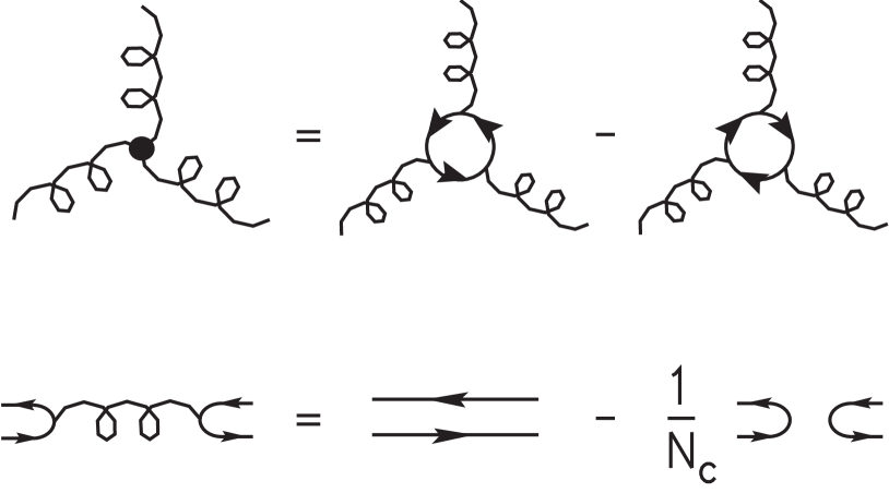
Figure 1: Diagrammatic equations for simplifying $SU(N_{c})$ color algebra. Curly lines (“gluon propagators”) represent adjoint indices, oriented solid lines (“quark propagators”) represent fundamental indices, and “quark-gluon vertices” represent the generator matrices $(T^{a})_{i}^{~{}{\bar{\jmath}}}$.

It is easy to see that any tree diagram for $n$-gluon scattering can be reduced to a sum of “single trace” terms. This observation leads to the color decomposition of the the $n$-gluon tree amplitude,$\!{}^{{\bf?}}$

$${\cal A}^{\rm tree}_{n}\left(\{k_{i},\lambda_{i},a_{i}\}\right)=g^{n-2}\hskip-3.69885pt\sum_{\sigma\in S_{n}/Z_{n}}\hskip-3.69885pt\mathop{\rm Tr}\nolimits\left(T^{a_{\sigma(1)}}\cdots T^{a_{\sigma(n)}}\right)\ A_{n}^{\rm tree}(\sigma(1^{\lambda_{1}}),\ldots,\sigma(n^{\lambda_{n}})).$$ (4)

Here $g$ is the gauge coupling (${g^{2}\over 4\pi}=\alpha_{s}$), $k_{i},\lambda_{i}$ are the gluon momenta and helicities, and $A_{n}^{\rm tree}(1^{\lambda_{1}},\ldots,n^{\lambda_{n}})$ are the partial amplitudes, which contain all the kinematic information. $S_{n}$ is the set of all permutations of $n$ objects, while $Z_{n}$ is the subset of cyclic permutations, which preserves the trace; one sums over the set $S_{n}/Z_{n}$ in order to sweep out all distinct cyclic orderings in the trace. The real work is still to come, in calculating the independent partial amplitudes $A_{n}^{\rm tree}$. However, the partial amplitudes are simpler than the full amplitude because they are color-ordered: they only receive contributions from diagrams with a particular cyclic ordering of the gluons. Because of this, the singularities of the partial amplitudes, poles and (in the loop case) cuts, can only occur in a limited set of momentum channels, those made out of sums of cyclically adjacent momenta. For example, the five-point partial amplitudes $A_{5}^{\rm tree}(1^{\lambda_{1}},2^{\lambda_{2}},3^{\lambda_{3}},4^{\lambda_{4}},5^{\lambda_{5}})$ can only have poles in $s_{12}$, $s_{23}$, $s_{34}$, $s_{45}$, and $s_{51}$, and not in $s_{13}$, $s_{24}$, $s_{35}$, $s_{41}$, or $s_{52}$, where $s_{ij}\equiv(k_{i}+k_{j})^{2}$.

Similarly, tree amplitudes ${\bar{q}}qgg\cdots g$ with two external quarks can be reduced to single strings of $T^{a}$ matrices,

$${\cal A}^{\rm tree}_{n}=g^{n-2}\hskip-3.69885pt\sum_{\sigma\in S_{n-2}}\hskip-3.69885pt\left(T^{a_{\sigma(3)}}\cdots T^{a_{\sigma(n)}}\right)_{i_{2}}^{~{}{\bar{\jmath}}_{1}}A_{n}^{\rm tree}(1_{\bar{q}}^{\lambda_{1}},2_{q}^{\lambda_{2}},\sigma(3^{\lambda_{3}}),\ldots,\sigma(n^{\lambda_{n}})),$$ (5)

where numbers without subscripts refer to gluons.

Exercise: Write down the color decomposition for the tree amplitude ${\bar{q}}q{\bar{Q}}Qg$.

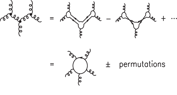
Figure 2: A sample diagram for tree-level five-gluon scattering, reduced to a single trace.

Color decompositions at loop level are equally straightforward. In Fig. 3 we simplify a sample diagram for four-gluon scattering at one loop. Again the $-1/N_{c}$ terms in Eq. 2 are not present, but now both single and double trace structures are generated, leading to the one-loop color decomposition,$\!{}^{{\bf?}}$

$$\hskip-22.76219pt{\cal A}^{\rm 1-loop}_{n}\left(\{k_{i},\lambda_{i},a_{i}\}\right)$$

$$\hskip 17.07164pt=g^{n}\Biggl{[}\sum_{\sigma\in S_{n}/Z_{n}}N_{c}\,\mathop{\rm Tr}\nolimits\left(T^{a_{\sigma(1)}}\cdots T^{a_{\sigma(n)}}\right)\ A_{n;1}(\sigma(1^{\lambda_{1}}),\ldots,\sigma(n^{\lambda_{n}}))$$

$$\hskip 42.67912pt+\ \sum_{c=2}^{\lfloor{n/2}\rfloor+1}\sum_{\sigma\in S_{n}/S_{n;c}}\mathop{\rm Tr}\nolimits\left(T^{a_{\sigma(1)}}\cdots T^{a_{\sigma(c-1)}}\right)\ \mathop{\rm Tr}\nolimits\left(T^{a_{\sigma(c)}}\cdots T^{a_{\sigma(n)}}\right)\$$

$$\hskip 150.79959pt\times\ A_{n;c}(\sigma(1^{\lambda_{1}}),\ldots,\sigma(n^{\lambda_{n}}))\Biggr{]}\,,$$ (6)

where $A_{n;c}$ are the partial amplitudes, $Z_{n}$ and $S_{n;c}$ are the subsets of $S_{n}$ that leave the corresponding single and double trace structures invariant, and $\lfloor x\rfloor$ is the greatest integer less than or equal to $x$.

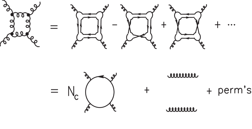
Figure 3: A diagram for one-loop four-gluon scattering, reduced to single and double traces.

The $A_{n;1}$ are the more basic objects in Eq. 6, and are called primitive amplitudes, because:

a. Like the tree partial amplitudes $A_{n}^{\rm tree}$ in Eq. 4, they are color-ordered.

b. It turns out that the remaining $A_{n;c>1}$ can be generated $\!{}^{{\bf?},{\bf?}}$ as sums of permutations of the $A_{n;1}$. (For amplitudes with external quarks as well as gluons, the primitive amplitudes are not a subset of the partial amplitudes; new color-ordered objects have to be defined.$\!{}^{{\bf?}}$)

One might worry that the color and helicity decompositions will lead to a huge proliferation in the number of primitive/partial amplitudes that have to be computed. Actually it is not too bad, thanks to symmetries such as parity — which allows one to simultaneously reverse all helicities in an amplitude — and charge conjugation — which allows one to exchange a quark and anti-quark, or equivalently flip the helicity on a quark line. For example, using parity and cyclic ($Z_{5}$) symmetry, the five-gluon amplitude has only four independent tree-level partial amplitudes:

$$A_{5}^{\rm tree}(1^{+},2^{+},3^{+},4^{+},5^{+}),\qquad\qquad A_{5}^{\rm tree}(1^{-},2^{+},3^{+},4^{+},5^{+}),$$

$$A_{5}^{\rm tree}(1^{-},2^{-},3^{+},4^{+},5^{+}),\qquad\qquad A_{5}^{\rm tree}(1^{-},2^{+},3^{-},4^{+},5^{+}).$$ (7)

In fact, we’ll see that the first two tree partial amplitudes vanish, and there is a group theory relation between the last two, so there is only one independent nonvanishing object to calculate. At one-loop there are four independent objects — Eq. 7 with $A_{5}^{\rm tree}$ replaced by $A_{5;1}$ — but only the last two contribute to the NLO cross-section, due to the tree-level vanishings.

The group theory relation just mentioned derives from the fact that the tree color decomposition, Eq. 4, is equally valid for gauge group $U(N_{c})$ as $SU(N_{c})$, but any amplitude containing the extra $U(1)$ photon must vanish. Hence if we substitute the $U(1)$ generator — the identity matrix — into the right-hand-side of Eq. 4, and collect the terms with the same remaining color structure, that linear combination of partial amplitudes must vanish. We get

$$0 = A_{n}^{\rm tree}(1,2,3,\ldots,n)+A_{n}^{\rm tree}(2,1,3,\ldots,n)+A_{n}^{\rm tree}(2,3,1,\ldots,n)$$ (8)

$$\hskip 28.45274pt+\cdots+A_{n}^{\rm tree}(2,3,\ldots,1,n),$$

often called a “photon decoupling equation”$\!{}^{{\bf?}}$ or “dual Ward identity”$\!{}^{{\bf?}}$ (because Eq. 8 can be derived from string theory, a.k.a. dual theory). In the five-point case, we can use Eq. 8 to get

$$A_{5}^{\rm tree}(1^{-},2^{+},3^{-},4^{+},5^{+}) = -A_{5}^{\rm tree}(1^{-},3^{-},2^{+},4^{+},5^{+})$$ (9)

$$-A_{5}^{\rm tree}(1^{-},3^{-},4^{+},2^{+},5^{+})$$

$$-A_{5}^{\rm tree}(1^{-},3^{-},4^{+},5^{+},2^{+}).$$

The partial amplitude where the two negative helicities are not adjacent has been expressed in terms of the partial amplitude where they are adjacent, as desired.

Since color is confined and unobservable, the QCD-improved parton model cross-sections of interest to us are averaged over initial colors and summed over final colors. These color sums can be performed very easily using the diagrammatic techniques. For example, Fig. 4 illustrates the evaluation of the color sums needed for the tree-level four-gluon cross-section. In this case we can use the much simpler $U(N_{c})$ color algebra, omitting the $-1/N_{c}$ term in Eq. 2, because the $U(1)$ contribution vanishes. (This shortcut is not valid for general loop amplitudes, or if external quarks are present.) Using also the reflection identity discussed below, Eq. 45, the total color sum becomes

$$\sum_{{\rm colors}}[{\cal A}_{4}^{{\rm tree}\,*}{\cal A}_{4}^{\rm tree}] = 2\,g^{4}\,A_{4}^{{\rm tree}\,*}(1,2,3,4)\times\biggl{[}A_{4}^{\rm tree}(1,2,3,4)(N_{c}^{4}+N_{c}^{2})$$ (10)

$$\quad+\Bigl{(}A_{4}^{\rm tree}(2,1,3,4)+A_{4}^{\rm tree}(2,3,1,4)\Bigr{)}(N_{c}^{2}+N_{c}^{2})\biggr{]}$$

$$\qquad\qquad+\ \hbox{2 more permutations}$$

$$= g^{4}\,N_{c}^{2}(N_{c}^{2}-1)\sum_{\sigma\in S_{3}}|A_{4}^{\rm tree}(\sigma(1),\sigma(2),\sigma(3),4)|^{2}\ ,$$

where we have used the decoupling identity, Eq. 8, in the last step.

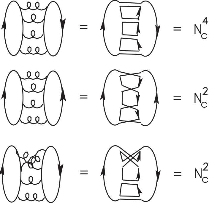
Figure 4: Diagrammatic evaluation of color sums for the tree-level four-gluon cross-section.

Because we have stripped all the color factors out of the partial amplitudes, the color-ordered Feynman rules for constructing these objects are purely kinematic (no $T^{a}$’s or $f^{abc}$’s are left). The rules are given in Fig. 5, for quantization in Lorentz-Feynman gauge. (Later we will discuss alternate gauges.) To compute a tree partial amplitude, or a color-ordered loop partial amplitude such as $A_{n;1}$,

1. Draw all color-ordered graphs, i.e. all planar graphs where the cyclic ordering of the external legs matches the ordering of the $T^{a_{i}}$ matrices in the corresponding color structure,

2. Evaluate each graph using the color-ordered vertices of Fig. 5.

Starting with the standard Feynman rules in terms of $f^{abc}$, etc., you can check that this prescription works because:

1) of all possible graphs, only the color-ordered graphs can contribute to the desired color structure, and

2) the color-ordered vertices are obtained by inserting Eq. 1 into the standard Feynman rules and extracting a single ordering of the $T^{a}$’s; hence they keep only the portion of a color-ordered graph which does contribute to the correct color structure.

Many partial amplitudes are not color-ordered — for example the $A_{n;c}$ for $c>1$ in Eq. 6 — and so the above rules do not apply. However, as mentioned above one can usually express such quantities as sums over permutations of color-ordered “primitive amplitudes” — for example the $A_{n;1}$ — to which the rules do apply.

Figure 5: Color-ordered Feynman rules, in Lorentz-Feynman gauge, omitting ghosts. Straight lines represent fermions, wavy lines gluons. All momenta are taken outgoing.

2.2 Helicity Nitty Gritty

The spinor helicity formalism for massless vector bosons $\!{}^{{\bf?},{\bf?},{\bf?}}$ is largely responsible for the existence of extremely compact representations of tree and loop partial amplitudes in QCD. It introduces a new set of kinematic objects, spinor products, which neatly capture the collinear behavior of these amplitudes. A (small) price to pay is that automated simplification of large expressions containing these objects is not always straightforward, because they obey nonlinear identities. In this section we will review the spinor helicity formalism and some of the key identities.

We begin with massless fermions. Positive and negative energy solutions of the massless Dirac equation are identical up to normalization conventions. One way to see this is to note that the positive and negative energy projection operators, $\Lambda_{+}(k)\sim u(k)\otimes\overline{u(k)}$ and $\Lambda_{-}(k)\sim v(k)\otimes\overline{v(k)}$, are both proportional to $\not{\hbox{\kern-2.3pt$k$}}$ in the massless limit. Thus the solutions of definite helicity, $u_{\pm}(k)=\textstyle{1\over 2}(1\pm\gamma_{5})u(k)$ and $v_{\mp}(k)=\textstyle{1\over 2}(1\pm\gamma_{5})v(k)$, can be chosen to be equal to each other. (For negative energy solutions, the helicity is the negative of the chirality or $\gamma_{5}$ eigenvalue.) A similar relation holds between the conjugate spinors $\overline{u_{\pm}(k)}=\overline{u(k)}\textstyle{1\over 2}(1\mp\gamma_{5})$ and $\overline{v_{\mp}(k)}=\overline{v(k)}\textstyle{1\over 2}(1\mp\gamma_{5})$. Since we will be interested in amplitudes with a large number of momenta, we label them by $k_{i}$, $i=1,2,\ldots,n$, and use the shorthand notation

$$|i^{\pm}\rangle\ \equiv\ |k_{i}^{\pm}\rangle\ \equiv\ u_{\pm}(k_{i})\ =\ v_{\mp}(k_{i}),\qquad\langle i^{\pm}|\equiv\ \langle k_{i}^{\pm}|\equiv\ \overline{u_{\pm}(k_{i})}\ =\ \overline{v_{\mp}(k_{i})}.$$ (11)

We define the basic spinor products by

$$\left\langle i\,j\right\rangle\ \equiv\ \langle i^{-}|j^{+}\rangle\ =\ \overline{u_{-}(k_{i})}u_{+}(k_{j}),\qquad\left[i\,j\right]\ \equiv\ \langle i^{+}|j^{-}\rangle\ =\ \overline{u_{+}(k_{i})}u_{-}(k_{j}).$$ (12)

The helicity projection implies that products like $\langle i^{+}|j^{+}\rangle$ vanish.

For numerical evaluation of the spinor products, it is useful to have explicit formulae for them, for some representation of the Dirac $\gamma$ matrices. In the Dirac representation,

$$\gamma^{0}\ =\ \left(\matrix{{\bf 1}&{\bf 0}\cr{\bf 0}&-{\bf 1}\cr}\right)\ ,\qquad\gamma^{i}\ =\ \left(\matrix{{\bf 0}&{\bf\sigma}^{i}\cr-{\bf\sigma}^{i}&{\bf 0}\cr}\right)\ ,\qquad\gamma_{5}\ =\ \left(\matrix{{\bf 0}&{\bf 1}\cr{\bf 1}&{\bf 0}\cr}\right)\ ,$$ (13)

the massless spinors can be chosen as follows,

$$u_{+}(k)=v_{-}(k)={1\over\sqrt{2}}\left[\matrix{\sqrt{k^{+}}\cr\sqrt{k^{-}}e^{i\varphi_{k}}\cr\sqrt{k^{+}}\cr\sqrt{k^{-}}e^{i\varphi_{k}}\cr}\right],\hskip 8.53581ptu_{-}(k)=v_{+}(k)={1\over\sqrt{2}}\left[\matrix{\sqrt{k^{-}}e^{-i\varphi_{k}}\cr-\sqrt{k^{+}}\cr-\sqrt{k^{-}}e^{-i\varphi_{k}}\cr\sqrt{k^{+}}\cr}\right],$$ (14)

where

$$e^{\pm i\varphi_{k}}\ \equiv\ {k^{1}\pm ik^{2}\over\sqrt{(k^{1})^{2}+(k^{2})^{2}}}\ =\ {k^{1}\pm ik^{2}\over\sqrt{k^{+}k^{-}}}\ ,\qquad k^{\pm}\ =\ k^{0}\pm k^{3}.$$ (15)

Exercise: Show that these solutions satisfy the massless Dirac equation with the proper chirality.

Plugging Eqs. 14 into the definitions of the spinor products, Eq. 12, we get explicit formulae for the case when both energies are positive,

$$\left\langle i\,j\right\rangle = \sqrt{k_{i}^{-}k_{j}^{+}}e^{i\varphi_{k_{i}}}-\sqrt{k_{i}^{+}k_{j}^{-}}e^{i\varphi_{k_{j}}}\ =\ \sqrt{|s_{ij}|}e^{i\phi_{ij}},$$

$$\left[i\,j\right] = -\sqrt{k_{i}^{-}k_{j}^{+}}e^{-i\varphi_{k_{i}}}+\sqrt{k_{i}^{+}k_{j}^{-}}e^{-i\varphi_{k_{j}}}\ =\ \sqrt{|s_{ij}|}e^{-i(\phi_{ij}+\pi)},$$ (16)

$$\qquad\qquad k_{i}^{0}>0,\quad k_{j}^{0}>0,$$

where $s_{ij}\ =\ (k_{i}+k_{j})^{2}\ =\ 2k_{i}\cdot k_{j}$, and

$$\cos\phi_{ij}\ =\ {k_{i}^{1}k_{j}^{+}-k_{j}^{1}k_{i}^{+}\over\sqrt{|s_{ij}|k_{i}^{+}k_{j}^{+}}}\ ,\qquad\sin\phi_{ij}\ =\ {k_{i}^{2}k_{j}^{+}-k_{j}^{2}k_{i}^{+}\over\sqrt{|s_{ij}|k_{i}^{+}k_{j}^{+}}}\ .$$ (17)

The spinor products are, up to a phase, square roots of Lorentz products. We’ll see that the collinear limits of massless gauge amplitudes have this kind of square-root singularity, which explains why spinor products lead to very compact analytic representations of gauge amplitudes, as well as improved numerical stability.

We would like the spinor products to have simple properties under crossing symmetry, i.e. as energies become negative.$\!{}^{{\bf?}}$ We define the spinor product $\left\langle i\,j\right\rangle$ by analytic continuation from the positive energy case, using the same formula, Eq. 16, but with $k_{i}$ replaced by $-k_{i}$ if $k_{i}^{0}<0$, and similarly for $k_{j}$; and with an extra multiplicative factor of $i$ for each negative energy particle. We define $\left[i\,j\right]$ through the identity

$$\left\langle i\,j\right\rangle\left[j\,i\right]=\langle i^{-}|j^{+}\rangle\langle j^{+}|i^{-}\rangle=\mathop{\rm tr}\nolimits\bigl{(}\textstyle{1\over 2}(1-\gamma_{5})\not{\hbox{\kern-2.3pt$k$}}_{i}\not{\hbox{\kern-2.3pt$k$}}_{j}\bigr{)}=2k_{i}\cdot k_{j}=s_{ij}.$$ (18)

We also have the useful identities:

Gordon identity and projection operator:

$$\langle i^{\pm}|\gamma^{\mu}|i^{\pm}\rangle\ =\ 2k_{i}^{\mu},\qquad\qquad|i^{\pm}\rangle\langle i^{\pm}|\ =\ \textstyle{1\over 2}(1\pm\gamma_{5})\not{\hbox{\kern-2.3pt$k$}}_{i}$$ (19)

antisymmetry:

$$\left\langle j\,i\right\rangle=-\left\langle i\,j\right\rangle,\qquad\left[j\,i\right]=-\left[i\,j\right],\qquad\left\langle i\,i\right\rangle=\left[i\,i\right]=0\qquad$$ (20)

Fierz rearrangement:

$$\langle i^{+}|\gamma^{\mu}|j^{+}\rangle\langle k^{+}|\gamma_{\mu}|l^{+}\rangle\ =\ 2\,\left[i\,k\right]\left\langle l\,j\right\rangle$$ (21)

charge conjugation of current:

$$\langle i^{+}|\gamma^{\mu}|j^{+}\rangle\ =\ \langle j^{-}|\gamma^{\mu}|i^{-}\rangle$$ (22)

Schouten identity:

$$\left\langle i\,j\right\rangle\left\langle k\,l\right\rangle\ =\ \left\langle i\,k\right\rangle\left\langle j\,l\right\rangle+\left\langle i\,l\right\rangle\left\langle k\,j\right\rangle.$$ (23)

In an $n$-point amplitude, momentum conservation, $\sum_{i=1}^{n}k_{i}^{\mu}=0$, provides one more identity,

$$\sum_{{{i=1}\atop{i\neq j,k}}}^{n}\left[j\,i\right]\left\langle i\,k\right\rangle\ =\ 0.$$ (24)

The next step is to introduce a spinor representation for the polarization vector for a massless gauge boson of definite helicity $\pm 1$,

$$\varepsilon^{\pm}_{\mu}(k,q)\ =\ \pm{\langle q^{\mp}|\gamma_{\mu}|k^{\mp}\rangle\over\sqrt{2}\langle q^{\mp}|k^{\pm}\rangle}\ ,$$ (25)

where $k$ is the vector boson momentum and $q$ is an auxiliary massless vector, called the reference momentum, reflecting the freedom of on-shell gauge tranformations. We will not motivate Eq. 25, but just show that it has the desired properties. Since $\not{\hbox{\kern-2.3pt$k$}}|k^{\pm}\rangle=0$, $\varepsilon^{\pm}(k,q)$ is transverse to $k$, for any $q$,

$$\varepsilon^{\pm}(k,q)\cdot k\ =\ 0.$$ (26)

Complex conjugation reverses the helicity,

$$(\varepsilon_{\mu}^{+})^{*}\ =\ \varepsilon_{\mu}^{-}\ .$$ (27)

The denominator gives $\varepsilon_{\mu}$ the standard normalization (using Eq. 21),

$$\varepsilon^{+}\cdot(\varepsilon^{+})^{*} = \varepsilon^{+}\cdot\varepsilon^{-}\ =\ -{1\over 2}{\langle q^{-}|\gamma_{\mu}|k^{-}\rangle\langle q^{+}|\gamma^{\mu}|k^{+}\rangle\over\left\langle q\,k\right\rangle\left[q\,k\right]}\ =\ -1,$$

$$\varepsilon^{+}\cdot(\varepsilon^{-})^{*} = \varepsilon^{+}\cdot\varepsilon^{+}\ =\ {1\over 2}{\langle q^{-}|\gamma_{\mu}|k^{-}\rangle\langle q^{-}|\gamma^{\mu}|k^{-}\rangle\over{\left\langle q\,k\right\rangle}^{2}}\ =\ 0.$$ (28)

States with helicity $\pm 1$ are produced by $\varepsilon^{\pm}$. The easiest way to see this is to consider a rotation around the ${\bf k}$ axis, and notice that the $|k^{+}\rangle$ in the denominator of Eq. 25 picks up the opposite phase from the state $|k^{-}\rangle$ in the numerator; i.e. it doubles the phase from that appropriate for a spinor (helicity $+\textstyle{1\over 2}$) to that appropriate for a vector (helicity $+1$). Finally, changing the reference momentum $q$ does amount to an on-shell gauge transformation, since $\varepsilon_{\mu}$ shifts by an amount proportional to $k_{\mu}$:

$$\varepsilon_{\mu}^{+}({\tilde{q}})-\varepsilon_{\mu}^{+}(q)\hskip-3.41432pt = \hskip-3.41432pt{\langle{\tilde{q}}^{-}|\gamma_{\mu}|k^{-}\rangle\over\sqrt{2}\left\langle{\tilde{q}}\,k\right\rangle}-{\langle q^{-}|\gamma_{\mu}|k^{-}\rangle\over\sqrt{2}\left\langle q\,k\right\rangle}=-{\langle{\tilde{q}}^{-}|\gamma_{\mu}\not{\hbox{\kern-2.3pt$k$}}|q^{+}\rangle+\langle{\tilde{q}}^{-}|\not{\hbox{\kern-2.3pt$k$}}\gamma_{\mu}|q^{+}\rangle\over\sqrt{2}\left\langle{\tilde{q}}\,k\right\rangle\left\langle q\,k\right\rangle}$$ (29)

$$= \hskip-3.41432pt-{\sqrt{2}\left\langle{\tilde{q}}\,q\right\rangle\over\left\langle{\tilde{q}}\,k\right\rangle\left\langle q\,k\right\rangle}\times k_{\mu}\ .$$

Exercise: Show that the completeness relation for these polarization vectors is that of an light-like axial gauge,

$$\sum_{\lambda=\pm}\varepsilon^{\lambda}_{\mu}(k,q)\,(\varepsilon^{\lambda}_{\nu}(k,q))^{*}\ =\ -\eta_{\mu\nu}+{k_{\mu}q_{\nu}+k_{\nu}q_{\mu}\over k\cdot q}\ .$$ (30)

A separate reference momentum $q_{i}$ can be chosen for each gluon momentum $k_{i}$ in an amplitude. Because it is a gauge choice, one should be careful not to change the $q_{i}$ within the calculation of a gauge-invariant quantity (such as a partial amplitude). On the other hand, different choices can be made when calculating different gauge-invariant quantities. A judicious choice of the $q_{i}$ can simplify a calculation substantially, by making many terms and diagrams vanish, due primarily to the following identities, where $\varepsilon_{i}^{\pm}(q)\equiv\varepsilon^{\pm}(k_{i},q_{i}=q)$:

$$\varepsilon_{i}^{\pm}(q)\cdot q = 0,$$ (31)

$$\varepsilon_{i}^{+}(q)\cdot\varepsilon_{j}^{+}(q) = \varepsilon_{i}^{-}(q)\cdot\varepsilon_{j}^{-}(q)\ =\ 0,$$ (32)

$$\varepsilon_{i}^{+}(k_{j})\cdot\varepsilon_{j}^{-}(q) = \varepsilon_{i}^{+}(q)\cdot\varepsilon_{j}^{-}(k_{i})\ =\ 0,$$ (33)

$$\not{\hbox{\kern-2.3pt$\varepsilon$}}_{i}^{+}(k_{j})|j^{+}\rangle = \not{\hbox{\kern-2.3pt$\varepsilon$}}_{i}^{-}(k_{j})|j^{-}\rangle\ =\ 0,$$ (34)

$$\langle j^{+}|\not{\hbox{\kern-2.3pt$\varepsilon$}}_{i}^{-}(k_{j}) = \langle j^{-}|\not{\hbox{\kern-2.3pt$\varepsilon$}}_{i}^{+}(k_{j})\ =\ 0.$$ (35)

In particular, it is useful to choose the reference momenta of like-helicity gluons to be identical, and to equal the external momentum of one of the opposite-helicity set of gluons.

We can now express any amplitude with massless external fermions and vector bosons in terms of spinor products. Since these products are defined for both positive- and negative-energy four-momenta, we can use crossing symmetry to extract a number of scattering amplitudes from the same expression, by exchanging which momenta are outgoing and which incoming. However, because the helicity of a positive-energy (negative-energy) massless spinor has the same (opposite) sign as its chirality, the helicities assigned to the particles — bosons as well as fermions — depend on whether they are incoming or outgoing. Our convention is to label particles with their helicity when they are considered outgoing (positive-energy); if they are incoming the helicity is reversed.

The spinor-product representation of an amplitude can be related to a more conventional one in terms of Lorentz-invariant objects, the momentum invariants $k_{i}\cdot k_{j}$ and contractions of the Levi-Civita tensor $\varepsilon_{\mu\nu\sigma\rho}$ with external momenta. The spinor products carry around a number of phases. Some of the phases are unphysical because they are associated with external-state conventions, such as the definitions of the spinors $|i^{\pm}\rangle$. Physical quantities such as cross-sections (or amplitudes from which an overall phase has been removed), when constructed out of the spinor products, will be independent of such choices. Thus for each external momentum label $i$, if the product $\left\langle i\,j\right\rangle$ appears then its phase should be compensated by some $\left[i\,k\right]$ (or equivalently $1/\left\langle i\,k\right\rangle=-\left[i\,k\right]/s_{ik}$). If a spinor string appears in a physical quantity, then it must terminate, i.e. it has the form

$$\left\langle i_{1}\,i_{2}\right\rangle\left[i_{2}\,i_{3}\right]\left\langle i_{3}\,i_{4}\right\rangle\cdots\left[i_{2m}\,i_{1}\right],$$ (36)

for some $m$. Multiplying Eq. 36 by $1=\left[i_{4}\,i_{1}\right]\left\langle i_{1}\,i_{4}\right\rangle/s_{i_{1}i_{4}}$, etc., we can break up any spinor string into strings of length two and four; the former are just $s_{ij}$’s (Eq. 18), while the latter can then be evaluated by performing the Dirac trace:

$$\left\langle i\,j\right\rangle\left[j\,l\right]\left\langle l\,m\right\rangle\left[m\,i\right] = \mathop{\rm tr}\nolimits\Bigl{(}\textstyle{1\over 2}(1-\gamma_{5})\not{\hbox{\kern-2.3pt$k$}}_{i}\not{\hbox{\kern-2.3pt$k$}}_{j}\not{\hbox{\kern-2.3pt$k$}}_{l}\not{\hbox{\kern-2.3pt$k$}}_{m}\Bigr{)}$$

$$= {1\over 2}\biggl{[}s_{ij}s_{lm}-s_{il}s_{jm}+s_{im}s_{jl}-4i\varepsilon(i,j,l,m)\biggr{]},$$ (37)

where $\varepsilon(i,j,l,m)\ =\ \varepsilon_{\mu\nu\sigma\rho}k_{i}^{\mu}k_{j}^{\nu}k_{l}^{\rho}k_{m}^{\sigma}$. Thus the Levi-Civita contractions are always accompanied by an $i$ and account for the physical phases. In practice, the spinor products offer the most compact representation of helicity amplitudes, but it is useful to know the connection to a more conventional representation.

Exercise: Verify the Schouten identity, Eq. 23, by multiplying both sides by $\left[j\,k\right]\left[l\,i\right]$ and using Eq. 37 to simplify.

3 Tree-level techniques

Now we are ready to attack some tree amplitudes, beginning with direct calculation of some simple examples, followed by a discussion of recursive techniques for generating more complicated amplitudes, and of the role of supersymmetry and factorization properties in tree-level QCD.

3.1 Simple examples

Let’s first compute the four-gluon tree helicity amplitude $A_{4}^{\rm tree}(1^{+},2^{+},3^{+},4^{+})$. Since all the gluons have the same helicity, if we choose all the reference momenta to be the same null-vector $q$ we can make all the $\varepsilon_{i}^{+}\cdot\varepsilon_{j}^{+}$ terms vanish according to Eq. 32. We can’t choose $q$ to equal one of the external momenta, because that polarization vector would have a singular denominator. But we could choose for example the null-vector $q^{\mu}=-2s_{23}k_{1}^{\mu}+(s_{12}-s_{23})(2k_{2}^{\mu}+k_{3}^{\mu})$. Actually we won’t need the explicit expression for $q$ here, because when we start to evaluate the various diagrams, we find that they always contain at least one $\varepsilon_{i}\cdot\varepsilon_{j}$, and therefore every diagram in this helicity amplitude vanishes identically!

This result generalizes easily to more external gluons. Each nonabelian vertex can contribute at most one momentum vector $k_{i}$ to the numerator algebra of the graph, and there are at most $n-2$ vertices. Thus there are at most $n-2$ momentum vectors available to contract with the $n$ polarization vectors $\varepsilon_{i}$ (the amplitude is linear in each $\varepsilon_{i}$). This means there must be at least one $\varepsilon_{i}\cdot\varepsilon_{j}$ contraction, and so the tree amplitude must vanish whenever we can arrange that all the $\varepsilon_{i}\cdot\varepsilon_{j}$ vanish. Obviously this can be arranged for the $n$-gluon amplitudes with all helicities the same, $A_{n}^{\rm tree}(1^{+},2^{+},3^{+},\ldots,n^{+})$, by again taking all the reference momenta to be identical. And it can be arranged for $A_{n}^{\rm tree}(1^{-},2^{+},3^{+},\ldots,n^{+})$ by the reference momentum choice $q_{2}=q_{3}=\cdots=q_{n}=k_{1}$, $q_{1}=k_{n}$. Thus we have already computed a large number of (zero) amplitudes,

$$A_{n}^{\rm tree}(1^{\pm},2^{+},3^{+},\ldots,n^{+})\ =\ 0.$$ (38)

Exercise: Use an analogous argument to show that the following ${\bar{q}}qgg\ldots g$ helicity amplitudes also vanish:

$$A_{n}^{\rm tree}(1_{\bar{q}}^{-},2_{q}^{+},3^{+},4^{+},\ldots,n^{+})\ =\ 0.$$ (39)

We’ll see later that an “effective” supersymmetry $\!{}^{{\bf?}}$ of tree-level QCD is responsible for all these vanishings.

Next we turn to the (nonzero) helicity amplitude $A_{4}^{\rm tree}(1^{-},2^{-},3^{+},4^{+})$, choosing the reference momenta $q_{1}=q_{2}=k_{4}$, $q_{3}=q_{4}=k_{1}$, so that only the contraction $\varepsilon_{2}^{-}\cdot\varepsilon_{3}^{+}$ is nonzero. It is easy to see from the color-ordered rules in Fig. 5 that only one of the three potential graphs contributes, the one with a gluon exchange in the $s_{12}$ channel. We get

$$\hskip-11.38109ptA_{4}^{\rm tree}(1^{-},2^{-},3^{+},4^{+})$$ (40)

$$= \left({i\over\sqrt{2}}\right)^{2}\left({-i\over s_{12}}\right)$$

$$\hskip 0.0pt\times\left[\varepsilon_{1}^{-}\cdot\varepsilon_{2}^{-}(k_{1}-k_{2})^{\mu}+(\varepsilon_{2}^{-})^{\mu}\varepsilon_{1}^{-}\cdot(2k_{2}+k_{1})+(\varepsilon_{1}^{-})^{\mu}\varepsilon_{2}^{-}\cdot(-2k_{1}-k_{2})\right]$$

$$\hskip 0.0pt\times\left[\varepsilon_{3}^{+}\cdot\varepsilon_{4}^{+}(k_{3}-k_{4})_{\mu}+(\varepsilon_{4}^{+})_{\mu}\varepsilon_{3}^{+}\cdot(2k_{4}+k_{3})+(\varepsilon_{3}^{+})_{\mu}\varepsilon_{4}^{+}\cdot(-2k_{3}-k_{4})\right]$$

$$= -{2i\over s_{12}}\bigl{(}\varepsilon_{2}^{-}\cdot\varepsilon_{3}^{+}\bigr{)}\bigl{(}\varepsilon_{1}^{-}\cdot k_{2}\bigr{)}\bigl{(}\varepsilon_{4}^{+}\cdot k_{3}\bigr{)}$$

$$= -{2i\over s_{12}}\left(-{2\over 2}{\left[4\,3\right]\left\langle 1\,2\right\rangle\over\left[4\,2\right]\left\langle 1\,3\right\rangle}\right)\left(-{\left[4\,2\right]\left\langle 2\,1\right\rangle\over\sqrt{2}\left[4\,1\right]}\right)\left(+{\left\langle 1\,3\right\rangle\left[3\,4\right]\over\sqrt{2}\left\langle 1\,4\right\rangle}\right)$$

$$= -i\,{\left\langle 1\,2\right\rangle{\left[3\,4\right]}^{2}\over\left[1\,2\right]\left\langle 1\,4\right\rangle\left[1\,4\right]}\ .$$

We can pretty up the answer a bit, using antisymmetry (Eq. 20), momentum conservation (Eq. 24), and $s_{34}=s_{12}$,

$$A_{4}^{\rm tree}(1^{-},2^{-},3^{+},4^{+}) = -i\,{\left\langle 1\,2\right\rangle(\left\langle 2\,3\right\rangle\left[3\,4\right])(\left[3\,4\right]\left\langle 3\,4\right\rangle)\over\left[1\,2\right]\left\langle 2\,3\right\rangle\left\langle 3\,4\right\rangle\left\langle 1\,4\right\rangle\left[1\,4\right]}$$ (41)

$$= i\,{\left\langle 1\,2\right\rangle(-\left\langle 2\,1\right\rangle\left[1\,4\right])(\left[1\,2\right]\left\langle 1\,2\right\rangle)\over\left[1\,2\right]\left\langle 2\,3\right\rangle\left\langle 3\,4\right\rangle\left\langle 4\,1\right\rangle\left[1\,4\right]}$$

$$= i\,{{\left\langle 1\,2\right\rangle}^{3}\over\left\langle 2\,3\right\rangle\left\langle 3\,4\right\rangle\left\langle 4\,1\right\rangle}\ ,$$

or

$$A_{4}^{\rm tree}(1^{-},2^{-},3^{+},4^{+})\ =\ i\,{{\left\langle 1\,2\right\rangle}^{4}\over\left\langle 1\,2\right\rangle\left\langle 2\,3\right\rangle\left\langle 3\,4\right\rangle\left\langle 4\,1\right\rangle}\ .$$ (42)

The remaining four-gluon helicity amplitude can be obtained from the decoupling identity, Eq. 8:

$$A_{4}^{\rm tree}(1^{-},2^{+},3^{-},4^{+}) = -A_{4}^{\rm tree}(1^{-},3^{-},2^{+},4^{+})-A_{4}^{\rm tree}(1^{-},3^{-},4^{+},2^{+})$$ (43)

$$= -i\,\left[{{\left\langle 1\,3\right\rangle}^{3}\over\left\langle 3\,2\right\rangle\left\langle 2\,4\right\rangle\left\langle 4\,1\right\rangle}+{{\left\langle 1\,3\right\rangle}^{3}\over\left\langle 3\,4\right\rangle\left\langle 4\,2\right\rangle\left\langle 2\,1\right\rangle}\right]$$

$$= i\,{{\left\langle 1\,3\right\rangle}^{3}(\left\langle 1\,2\right\rangle\left\langle 3\,4\right\rangle+\left\langle 1\,4\right\rangle\left\langle 2\,3\right\rangle)\over\left\langle 1\,2\right\rangle\left\langle 2\,3\right\rangle\left\langle 3\,4\right\rangle\left\langle 4\,1\right\rangle\left\langle 2\,4\right\rangle}\ ,$$

or using the Schouten identity, Eq. 23,

$$A_{4}^{\rm tree}(1^{-},2^{+},3^{-},4^{+})\ =\ i\,{{\left\langle 1\,3\right\rangle}^{4}\over\left\langle 1\,2\right\rangle\left\langle 2\,3\right\rangle\left\langle 3\,4\right\rangle\left\langle 4\,1\right\rangle}\ .$$ (44)

There are no other four-gluon amplitudes to compute, because parity allows one to reverse all helicities simultaneously, by exchanging $\left\langle\,\right\rangle\leftrightarrow\left[\,\right]$ and multiplying by $-1$ if there are an odd number of gluons.

Note also that the antisymmetry of the color-ordered rules implies that the partial amplitudes (even with external quarks) obey a reflection identity,

$$A_{n}^{\rm tree}(1,2,\ldots,n)\ =(-1)^{n}\ A_{n}^{\rm tree}(n,\ldots,2,1).$$ (45)

To obtain the unpolarized, color-summed cross-section for four-gluon scattering, we insert the nonvanishing helicity amplitudes, Eqs. 42 and 44, into Eq. 10, and sum over the negative helicity gluons $i,j$:

$$\sum_{{{\rm colors}\atop{\rm helicities}}}[{\cal A}_{4}^{{\rm tree}\,*}{\cal A}_{4}^{\rm tree}]\hskip-4.2679pt = \hskip-4.2679ptg^{4}\,N_{c}^{2}(N_{c}^{2}-1)\sum_{i>j=1}^{4}\sum_{\sigma\in S_{3}}{(s_{ij})^{4}\over s_{\sigma(1)\sigma(2)}s_{\sigma(2)\sigma(3)}s_{\sigma(3)4}s_{4\sigma(1)}}.$$

Of course polarized cross-sections can be constructed just as easily from the helicity amplitudes.

Next we calculate a sample five-parton tree amplitude, for two quarks and three gluons, $A_{5}^{\rm tree}(1_{\bar{q}}^{-},2_{q}^{+},3^{-},4^{+},5^{+})$, where the momenta without subscripts label the gluons. We choose the gluon reference momenta as $q_{3}=k_{2}$, $q_{4}=q_{5}=k_{1}$, so we can use the vanishing relations, Eqs. 34 and 35,

$$\langle 2^{+}|\not{\hbox{\kern-2.3pt$\varepsilon$}}_{3}^{-}\ =\ \not{\hbox{\kern-2.3pt$\varepsilon$}}_{4}^{+}|1^{+}\rangle\ =\ \not{\hbox{\kern-2.3pt$\varepsilon$}}_{5}^{+}|1^{+}\rangle\ =\ 0.$$ (47)

This kills the graphs where gluons 3 and 5 attach directly to the fermion line, and the graph with a four-gluon vertex, leaving only the two graphs shown in Fig. 6.

Figure 6: The two nonvanishing graphs in the ${\bar{q}}qggg$ helicity amplitude calculation.

Graph 1 evaluates to

$$-{i\over\sqrt{2}}{\langle 2^{+}|(\not{\hbox{\kern-2.3pt$k$}}_{3}-\not{\hbox{\kern-2.3pt$k$}}_{4}-\not{\hbox{\kern-2.3pt$k$}}_{5})|1^{+}\rangle\over s_{12}s_{45}}(\varepsilon_{3}^{-}\cdot\varepsilon_{5}^{+}\varepsilon_{4}^{+}\cdot k_{5}-\varepsilon_{3}^{-}\cdot\varepsilon_{4}^{+}\varepsilon_{5}^{+}\cdot k_{4})$$ (48)

$$= -i\,{\left[2\,3\right]\left\langle 3\,1\right\rangle\over s_{12}s_{45}}\left[-{\left[2\,5\right]\left\langle 1\,3\right\rangle\over\left[2\,3\right]\left\langle 1\,5\right\rangle}{\left\langle 1\,5\right\rangle\left[5\,4\right]\over\left\langle 1\,4\right\rangle}+{\left[2\,4\right]\left\langle 1\,3\right\rangle\over\left[2\,3\right]\left\langle 1\,4\right\rangle}{\left\langle 1\,4\right\rangle\left[4\,5\right]\over\left\langle 1\,5\right\rangle}\right]$$

$$= +i\,{\left[2\,3\right]{\left\langle 1\,3\right\rangle}^{2}\left[4\,5\right]\over s_{12}s_{45}\left[2\,3\right]\left\langle 1\,4\right\rangle\left\langle 1\,5\right\rangle}\Bigl{[}-\left\langle 1\,5\right\rangle\left[5\,2\right]-\left\langle 1\,4\right\rangle\left[4\,2\right]\Bigr{]}$$

$$= -i\,{\left[2\,3\right]{\left\langle 1\,3\right\rangle}^{3}\left[4\,5\right]\over s_{12}s_{45}\left\langle 1\,4\right\rangle\left\langle 1\,5\right\rangle}\ .$$

Graph 2 requires a few more uses of the spinor product identities (exercise):

$$\hskip-22.76219pt-{i\over\sqrt{2}s_{12}s_{34}}\Bigl{[}\langle 2^{+}|(\not{\hbox{\kern-2.3pt$k$}}_{3}+\not{\hbox{\kern-2.3pt$k$}}_{4}-\not{\hbox{\kern-2.3pt$k$}}_{5})|1^{+}\rangle\left(\textstyle{1\over 2}\varepsilon_{3}^{-}\cdot\varepsilon_{4}^{+}\varepsilon_{5}^{+}\cdot(k_{3}-k_{4})-\varepsilon_{3}^{-}\cdot\varepsilon_{5}^{+}\varepsilon_{4}^{+}\cdot k_{3}\right)$$ (49)

$$\qquad\qquad\qquad-\langle 2^{+}|(\not{\hbox{\kern-2.3pt$k$}}_{3}-\not{\hbox{\kern-2.3pt$k$}}_{4})|1^{+}\rangle\varepsilon_{3}^{-}\cdot\varepsilon_{4}^{+}\varepsilon_{5}^{+}\cdot(k_{3}+k_{4})\Bigr{]}$$

$$= \cdots\ =\ +i\,{\left[2\,5\right]{\left\langle 1\,3\right\rangle}^{3}\left[3\,4\right]\over s_{12}s_{34}\left\langle 1\,4\right\rangle\left\langle 1\,5\right\rangle}\ .$$

The sum is

$$A_{5}^{\rm tree}(1_{\bar{q}}^{-},2_{q}^{+},3^{-},4^{+},5^{+})=-i\,{{\left\langle 1\,3\right\rangle}^{3}\left(-\left[2\,3\right]\left\langle 3\,4\right\rangle-\left[2\,5\right]\left\langle 5\,4\right\rangle\right)\over s_{12}\left\langle 1\,4\right\rangle\left\langle 1\,5\right\rangle\left\langle 3\,4\right\rangle\left\langle 4\,5\right\rangle}\ ,$$ (50)

or

$$A_{5}^{\rm tree}(1_{\bar{q}}^{-},2_{q}^{+},3^{-},4^{+},5^{+})\ =\ i\,{{\left\langle 1\,3\right\rangle}^{3}\left\langle 2\,3\right\rangle\over\left\langle 1\,2\right\rangle\left\langle 2\,3\right\rangle\left\langle 3\,4\right\rangle\left\langle 4\,5\right\rangle\left\langle 5\,1\right\rangle}\ .$$ (51)

Once again the expression collapses to a single term. Spurious singularities associated with the reference momentum choice — such as $1/\left\langle 1\,4\right\rangle$ in the above example — are present in individual graphs but cancel out in the gauge-invariant sum.

3.2 Recursive Techniques

By now you can see that color-ordering, plus the spinor helicity formalism, can vastly reduce the number of diagrams, and terms per diagram, that have to be evaluated. However, with more external legs the results still get more complex and difficult to carry out by hand. Fortunately, a technique is available for generating tree amplitudes recursively in the number of legs.$\!{}^{{\bf?}}$ Even if one cannot simplify analytically the expressions obtained in this way, the recursive approach lends itself to efficient numerical evaluation.

In order to get a tree-level recursion relation, we need to construct an auxiliary quantity with one leg off-shell. For the construction of pure-glue amplitudes, we define the off-shell current $J^{\mu}(1,2,\ldots,n)$ to be the sum of color-ordered ($n+1)$-point Feynman graphs, where legs $1,2,\ldots,n$ are on-shell gluons, and leg “$\mu$” is off-shell, as shown in Fig. 7. The uncontracted vector index on the off-shell leg is also denoted by $\mu$; the off-shell propagator is defined to be included in $J^{\mu}$. Since $J^{\mu}$ is an off-shell quantity, it is gauge-dependent. For example, $J^{\mu}$ depends on the reference momenta for the on-shell gluons, which must therefore be kept fixed until after one has extracted an on-shell result. One can also construct amplitudes with external quarks recursively, by introducing an off-shell quark current $\!{}^{{\bf?}}$ as well as the gluon current $J^{\mu}$, but we will not do so here.

Figure 7: The off-shell gluon current $J^{\mu}(1,2,\ldots,n)$. Leg “$\mu$” is the only off-shell leg.

It is easy to write down a recursion relation for $J^{\mu}$, by following the off-shell line back into the diagram. One first encounters either a three-gluon vertex or a four-gluon vertex. Each of the off-shell lines branching out from this vertex attaches to a smaller number of on-shell gluons, thus we have the recursion relation$\!{}^{{\bf?}}$ depicted in Fig. 8,

$$\hskip 0.0ptJ^{\mu}(1,\ldots,n)\hskip-4.2679pt = \hskip-4.2679pt{-i\over P^{2}_{1,n}}\Biggl{[}\sum_{i=1}^{n-1}V_{3}^{\mu\nu\rho}(P_{1,i},P_{i+1,n})\ J_{\nu}(1,\ldots,i)\ J_{\rho}(i+1,\ldots,n)$$

$$\hskip-14.22636pt+\sum_{j=i+1}^{n-1}\sum_{i=1}^{n-2}V_{4}^{\mu\nu\rho\sigma}\ J_{\nu}(1,\ldots,i)\ J_{\rho}(i+1,\ldots,j)\ J_{\sigma}(j+1,\ldots,n)\Biggr{]},$$

where the $V_{i}$ are just the color-ordered gluon self-interactions,

$$V_{3}^{\mu\nu\rho}(P,Q) = {i\over\sqrt{2}}\left(\eta^{\nu\rho}(P-Q)^{\mu}+2\eta^{\rho\mu}Q^{\nu}-2\eta^{\mu\nu}P^{\rho}\right),$$

$$V_{4}^{\mu\nu\rho\sigma} = {i\over 2}\left(2\eta^{\mu\rho}\eta^{\nu\sigma}-\eta^{\mu\nu}\eta^{\rho\sigma}-\eta^{\mu\sigma}\eta^{\nu\rho}\right),$$ (53)

and

$$P_{i,j}\ \equiv\ k_{i}+k_{i+1}+\cdots+k_{j}.$$ (54)

The $J^{\mu}$ satisfy the photon decoupling relation,

$$J^{\mu}(1,2,3,\ldots,n)+J^{\mu}(2,1,3,\ldots,n)+\cdots+J^{\mu}(2,3,\ldots,n,1)\ =\ 0,$$ (55)

the reflection identity

$$J^{\mu}(1,2,3,\ldots,n)=\ (-1)^{n+1}\,J^{\mu}(n,\ldots,3,2,1),$$ (56)

and current conservation,

$$P^{\mu}_{1,n}\ J_{\mu}(1,2,\ldots,n)\ =\ 0.$$ (57)

Figure 8: The recursion relation for the off-shell gluon current $J^{\mu}(1,2,\ldots,n)$.

In some cases, the recursion relations can be solved in closed form.$\!{}^{{\bf?},{\bf?}}$ The simplest case is (as expected) when all on-shell gluons have the same helicity, for which we choose the common reference momentum $q$, and then

$$J^{\mu}(1^{+},2^{+},\ldots,n^{+})\ =\ {\langle q^{-}|\gamma^{\mu}\not{\hbox{\kern-2.3pt$P$}}_{1,n}|q^{+}\rangle\over\sqrt{2}\left\langle q\,1\right\rangle\left\langle 1\,2\right\rangle\cdots\left\langle n-1,\,n\right\rangle\left\langle n\,q\right\rangle}\ .$$ (58)

Let’s verify that this expression solves Eq. LABEL:eq:Jrecursion. Note first that the $V_{4}$ term does not contribute at all, nor the first term in $V_{3}$, because after Fierzing we get a factor of $\left\langle q\,q\right\rangle=0$. Thus the right-hand side of Eq. LABEL:eq:Jrecursion becomes (using $\left\langle q\,q\right\rangle=0$ to commute and rearrange terms)

$${1\over\sqrt{2}P^{2}_{1,n}\left\langle q\,1\right\rangle\left\langle 1\,2\right\rangle\cdots\left\langle n-1,\,n\right\rangle\left\langle n\,q\right\rangle}\sum_{i=1}^{n-1}{\left\langle i,\,i+1\right\rangle\over\left\langle i\,q\right\rangle\left\langle q,\,i+1\right\rangle}$$ (59)

$$\times\Bigl{(}\langle q^{-}|\gamma^{\mu}\not{\hbox{\kern-2.3pt$P$}}_{i+1,n}|q^{+}\rangle\langle q^{-}|\not{\hbox{\kern-2.3pt$P$}}_{i+1,n}\not{\hbox{\kern-2.3pt$P$}}_{1,i}|q^{+}\rangle$$

$$\qquad-\langle q^{-}|\gamma^{\mu}\not{\hbox{\kern-2.3pt$P$}}_{1,i}|q^{+}\rangle\langle q^{-}|\not{\hbox{\kern-2.3pt$P$}}_{1,i}\not{\hbox{\kern-2.3pt$P$}}_{i+1,n}|q^{+}\rangle\Bigr{)}$$

$$= {\langle q^{-}|\gamma^{\mu}\not{\hbox{\kern-2.3pt$P$}}_{1,n}|q^{+}\rangle\over\sqrt{2}P^{2}_{1,n}\left\langle q\,1\right\rangle\left\langle 1\,2\right\rangle\cdots\left\langle n-1,\,n\right\rangle\left\langle n\,q\right\rangle}$$

$$\times\left[\sum_{i=1}^{n-1}{\left\langle i,\,i+1\right\rangle\over\left\langle i\,q\right\rangle\left\langle q,\,i+1\right\rangle}\langle q^{-}|\not{\hbox{\kern-2.3pt$P$}}_{i+1,n}\right]\not{\hbox{\kern-2.3pt$P$}}_{1,n}|q^{+}\rangle\ .$$

Using the identity

$$\sum_{i=1}^{n-1}{\left\langle i,\,i+1\right\rangle\over\left\langle i\,q\right\rangle\left\langle q,\,i+1\right\rangle}\langle q^{-}|\not{\hbox{\kern-2.3pt$P$}}_{i+1,n}\ =\ {\langle 1^{-}|\not{\hbox{\kern-2.3pt$P$}}_{1,n}\over\left\langle 1\,q\right\rangle}\ ,$$ (60)

we get the desired result, Eq. 58.

Exercise: Prove the identity, Eq. 60, by first proving the identity

$$\sum_{i=j}^{k-1}{\left\langle i,\,i+1\right\rangle\over\left\langle i\,q\right\rangle\left\langle q,\,i+1\right\rangle}\ =\ {\left\langle j\,k\right\rangle\over\left\langle j\,q\right\rangle\left\langle q\,k\right\rangle}\ .$$ (61)

The “eikonal” identity, Eq. 61, also plays a role in understanding the structure of the soft singularities of QED amplitudes, when these are obtained from QCD partial amplitudes by the replacement $T^{a}\to 1$ (see Sections 3.4 and 3.5).

The current where the first on-shell gluon has negative helicity can be obtained similarly,

$$J^{\mu}(1^{-},2^{+},\ldots,n^{+})\ =\ {\langle 1^{-}|\gamma^{\mu}\not{\hbox{\kern-2.3pt$P$}}_{2,n}|1^{+}\rangle\over\sqrt{2}\left\langle 1\,2\right\rangle\cdots\left\langle n\,1\right\rangle}\sum_{m=3}^{n}{\langle 1^{-}|\not{\hbox{\kern-2.3pt$k$}}_{m}\not{\hbox{\kern-2.3pt$P$}}_{1,m}|1^{+}\rangle\over P_{1,m-1}^{2}P_{1,m}^{2}}\ ,$$ (62)

where the reference momentum choice is $q_{1}=k_{2}$, $q_{2}=\cdots=q_{n}=k_{1}$.

Exercise: Show this.

Amplitudes with $(n+1)$ legs are obtained from the currents $J^{\mu}(1,2,\ldots,n)$ by amputating the off-shell propagator (multiplying by $i\,P^{2}_{1,n}$), contracting the $\mu$ index with the appropriate on-shell polarization vector $\varepsilon_{n+1}^{\mu}$, and taking $P^{2}_{1,n}=k_{n+1}^{2}\to 0$. In the case of $J^{\mu}(1^{+},2^{+},\ldots,n^{+})$, there is no $P^{2}_{1,n}$ pole in the current, so the amplitude must vanish for both helicities of gluon $(n+1)$, in accord with Eq. 38. In the case of $J^{\mu}(1^{-},2^{+},\ldots,n^{+})$, the pole term requirement picks out the term $m=n$ in Eq. 62. Using reference momentum $q_{n+1}=k_{n}$ for $\varepsilon_{n+1}^{-}$, we obtain (replacing $\not{\hbox{\kern-2.3pt$P$}}_{1,n}\to-\not{\hbox{\kern-2.3pt$k$}}_{n+1}$, etc.),

$$\hskip-42.67912ptA_{n+1}^{\rm tree}(1^{-},2^{+},\ldots,n^{+},(n+1)^{-})$$ (63)

$$= -i\,{\langle n^{+}|\gamma_{\mu}|(n+1)^{+}\rangle\over\sqrt{2}\left[n,\,n+1\right]}{\langle 1^{-}|\gamma^{\mu}\not{\hbox{\kern-2.3pt$P$}}_{1,n}|1^{+}\rangle\over\sqrt{2}\left\langle 1\,2\right\rangle\cdots\left\langle n\,1\right\rangle}{\langle 1^{-}|\not{\hbox{\kern-2.3pt$k$}}_{n}\not{\hbox{\kern-2.3pt$P$}}_{1,n}|1^{+}\rangle\over P^{2}_{1,n-1}}$$

$$= -i\,{\left\langle 1,\,n+1\right\rangle\over\left\langle 1\,2\right\rangle\cdots\left\langle n\,1\right\rangle}{\left\langle n+1,\,1\right\rangle\left\langle 1\,n\right\rangle\left[n,\,n+1\right]\left\langle n+1,\,1\right\rangle\over s_{n,n+1}}\ ,$$

or

$$A_{n}^{\rm tree}(1^{-},2^{-},3^{+},4^{+},\ldots,n^{+})\ =\ i\,{{\left\langle 1\,2\right\rangle}^{4}\over\left\langle 1\,2\right\rangle\cdots\left\langle n\,1\right\rangle}\ .$$ (64)

Applying the decoupling identity, Eq. 8, and the spinor identity, Eq. 61, it is easy to obtain the remaining maximally helicity violating (MHV) or Parke-Taylor $\!{}^{{\bf?}}$ helicity amplitudes,

$$A_{jk}^{\rm tree\ MHV}\ \equiv\ A_{n}^{\rm tree}(1^{+},\ldots,j^{-},\ldots,k^{-},\ldots,n^{+})\ =\ i\,{{\left\langle j\,k\right\rangle}^{4}\over\left\langle 1\,2\right\rangle\cdots\left\langle n\,1\right\rangle}\ .$$ (65)

These remarkably simple amplitudes were first conjectured by Parke and Taylor $\!{}^{{\bf?}}$ on the basis of their collinear limits (see below) and photon decoupling relations, and were rigorously proven correct by Berends and Giele $\!{}^{{\bf?}}$ using the above recursive approach. The other nonvanishing helicity configurations (beginning at $n=6$) are typically more complicated. The MHV amplitudes can be used as the basis of approximation schemes, however.$\!{}^{{\bf?}}$

3.3 Supersymmetry

What does supersymmetry have to do with a non-supersymmetric theory such as QCD? The answer is that tree-level QCD is “effectively” supersymmetric,$\!{}^{{\bf?}}$ and the “non-supersymmetry” only leaks in at the loop level. To see the supersymmetry of an $n$-gluon tree amplitude is simple: It has no loops in it, so it has no fermion loops in it. Therefore the fermions in the theory might as well be gluinos, i.e. at tree-level the theory might as well be super Yang-Mills theory. Tree amplitudes with quarks are also supersymmetric, but at the level of partial amplitudes: after the color information has been stripped off, there is nothing to distinguish a quark from a gluino. Supersymmetry leads to extra relations between amplitudes, supersymmetric Ward identities (SWI),$\!{}^{{\bf?}}$ which can be quite useful in saving computational labor.$\!{}^{{\bf?}}$

To derive supersymmetric Ward identities,$\!{}^{{\bf?},{\bf?}}$ we use the fact that the supercharge $Q$ annihilates the vacuum (we are considering exactly supersymmetric theories, not spontaneously or softly broken ones!),

$$0\ =\ \left\langle 0|[Q,\Phi_{1}\Phi_{2}\cdots\Phi_{n}]|0\right\rangle\ =\ \sum_{i=1}^{n}\left\langle 0|\Phi_{1}\cdots[Q,\Phi_{i}]\cdots\Phi_{n}|0\right\rangle\ .$$ (66)

When the fields $\Phi_{i}$ create helicity eigenstates, many of the $[Q,\Phi_{i}]$ terms can be arranged to vanish. To proceed, we need the precise commutation relations of the supercharge with the fields $g^{\pm}(k)$, $\Lambda^{\pm}(k)$, which create gluon and gluino states of momentum $k$ ($k^{2}=0$) and helicity $\pm$. We multiply $Q$ by a Grassmann spinor parameter $\bar{\eta}$, defining $Q(\eta)\equiv\bar{\eta}^{\alpha}Q_{\alpha}$, so that $Q(\eta)$ commutes with the Fermi fields as well as the Bose fields. The commutators have the form

$$\left[Q(\eta),g^{\pm}(k)\right] = \mp\Gamma^{\pm}(k,\eta)\,\Lambda^{\pm}(k),$$

$$\left[Q(\eta),\Lambda^{\pm}(k)\right] = \mp\Gamma^{\mp}(k,\eta)\,g^{\pm}(k),$$ (67)

where $\Gamma(k,\eta)$ is linear in $\eta$, and has its form constrained by the Jacobi identity for the supersymmetry algebra,

$$0\ =\ \left[\left[Q(\eta),Q(\zeta)\right],\Phi(k)\right]+\left[\left[Q(\zeta),\Phi(k)\right],Q(\eta)\right]+\left[\left[\Phi(k),Q(\eta)\right],Q(\zeta)\right]\ ,$$ (68)

where $\Phi(k)$ is either $g^{\pm}(k)$ or $\Lambda^{\pm}(k)$. Since $[Q(\eta),Q(\zeta)]=-2i\bar{\eta}\not{\hbox{\kern-2.3pt$P$}}\zeta$, we need

$$\Gamma^{+}(k,\eta)\Gamma^{-}(k,\zeta)+\Gamma^{-}(k,\eta)\Gamma^{+}(k,\zeta)\ =\ -2i\bar{\eta}\not{\hbox{\kern-2.3pt$k$}}\zeta.$$ (69)

A solution to Eq. 69, which also has the correct behavior under rotations around the ${\bf k}$ axis, is (cf. Eq. 19)

$$\Gamma^{+}(k,\eta)\ =\ \bar{\eta}u_{-}(k),\qquad\Gamma^{-}(k,\eta)\ =\ \bar{\eta}u_{+}(k)\ =\ \bar{u}_{-}(k)\eta.$$ (70)

Finally, we choose $\eta$ to be a Grassmann parameter $\theta$, multiplied by the spinor for an arbitrary massless vector $q$, and choose $q$ so as to simplify the identities (much like the choice of reference momentum in $\varepsilon_{\pm}^{\mu}(q)$). Then $\Gamma^{\pm}(k,\eta)$ become

$$\Gamma^{+}(k,q)\ =\ \theta\,\langle q^{+}|k^{-}\rangle\ =\ \theta\,\left[q\,k\right],\quad\Gamma^{-}(k,q)\ =\ \theta\,\langle q^{-}|k^{+}\rangle\ =\ \theta\,\left\langle q\,k\right\rangle.$$ (71)

The simplest case is the like-helicity one. We start with

$$0\hskip-5.69054pt = \hskip-5.69054pt\left\langle 0|[Q(\eta(q)),\Lambda_{1}^{+}g_{2}^{+}g_{3}^{+}\cdots g_{n}^{+}]|0\right\rangle$$ (72)

$$= \hskip-5.69054pt-\Gamma^{-}(k_{1},q)\,A_{n}(g_{1}^{+},g_{2}^{+},\ldots,g_{n}^{+})+\Gamma^{+}(k_{2},q)\,A_{n}(\Lambda_{1}^{+},\Lambda_{2}^{+},g_{3}^{+},\ldots,g_{n}^{+})$$

$$\quad+\cdots+\Gamma^{+}(k_{n},q)\,A_{n}(\Lambda_{1}^{+},g_{2}^{+},\ldots,g_{n-1}^{+},\Lambda_{n}^{+}).$$

Since massless gluinos, like quarks, have only helicity-conserving interactions in (super) QCD, all of the amplitudes but the first in Eq. 72 must vanish. Therefore so must the like-helicity amplitude $A_{n}(g_{1}^{+},g_{2}^{+},\ldots,g_{n}^{+})$. Similarly, with one negative helicity we get

$$0 = \left\langle 0|[Q(\eta(q)),\Lambda_{1}^{+}g_{2}^{-}g_{3}^{+}\cdots g_{n}^{+}]|0\right\rangle$$

$$= -\Gamma^{-}(k_{1},q)\,A_{n}(g_{1}^{+},g_{2}^{-},g_{3}^{+},\ldots,g_{n}^{+})-\Gamma^{-}(k_{2},q)\,A_{n}(\Lambda_{1}^{+},\Lambda_{2}^{-},g_{3}^{+},\ldots,g_{n}^{+}),$$

where we have omitted the vanishing fermion-helicity-violating amplitudes. Now we use the freedom to choose $q$, setting $q=k_{1}$ to show the second amplitude vanishes and setting $q=k_{2}$ to show the first vanishes. Thus we have recovered Eqs. 38 and 39.

With two negative helicities, we begin to relate nonzero amplitudes:

$$0 = \left\langle 0|[Q(\eta(q)),g_{1}^{-}g_{2}^{-}\Lambda_{3}^{+}g_{4}^{+}\cdots g_{n}^{+}]|0\right\rangle$$ (74)

$$= \Gamma^{-}(k_{1},q)\,A_{n}(\Lambda_{1}^{-},g_{2}^{-},\Lambda_{3}^{+},\ldots,g_{n}^{+})+\Gamma^{-}(k_{2},q)\,A_{n}(g_{1}^{-},\Lambda_{2}^{-},\Lambda_{3}^{+},\ldots,g_{n}^{+})$$

$$\quad-\Gamma^{-}(k_{3},q)\,A_{n}(g_{1}^{-},g_{2}^{-},g_{3}^{+},\ldots,g_{n}^{+}).$$

Choosing $q=k_{1}$, we get

$$A_{n}(g_{1}^{-},g_{2}^{-},g_{3}^{+},g_{4}^{+},\ldots,g_{n}^{+})\ =\ {\left\langle 1\,2\right\rangle\over\left\langle 1\,3\right\rangle}\times A_{n}(g_{1}^{-},\Lambda_{2}^{-},\Lambda_{3}^{+},g_{4}^{+},\ldots,g_{n}^{+}).$$ (75)

No perturbative approximations were made in deriving any of the above SWI; thus they hold order-by-order in the loop expansion. They apply directly to QCD tree amplitudes, because of their “effective” supersymmetry. But they can also be used to save some work at the loop level (see below). Since supersymmetry commutes with color, the SWI apply to each color-ordered partial amplitude separately. Summarizing the above “MHV” results (and similar ones including a pair of external scalar fields), we have

$$A_{n}^{\rm SUSY}(1^{\pm},2^{+},3^{+},\ldots,n^{+})\hskip-5.69054pt = \hskip-5.69054pt0,$$ (76)

$$A_{n}^{\rm SUSY}(1^{-},2_{P}^{-},3_{P}^{+},4^{+},\ldots,n^{+})\hskip-5.69054pt = \hskip-5.69054pt\left({\left\langle 1\,2\right\rangle\over\left\langle 1\,3\right\rangle}\right)^{2|h_{P}|}A_{n}^{\rm SUSY}(1^{-},2_{\phi}^{-},3_{\phi}^{+},4^{+},\ldots,n^{+}).$$

Here no subscript refers to a gluon, while $\phi$ refers to a scalar particle (for which the “helicity” $\pm$ means particle vs. antiparticle), and $P$ refers to a scalar, fermion or gluon, with respective helicity $h_{P}=0,\textstyle{1\over 2},1$.

We can use Eq. LABEL:eq:MHVSWI at the four-point level to obtain the ${\bar{q}}qgg$ amplitudes from the four-gluon ones, Eqs. 42 and 44:

$$A_{4}^{\rm tree}(1_{\bar{q}}^{-},2_{q}^{+},3^{-},4^{+}) = i\,{{\left\langle 1\,3\right\rangle}^{3}\left\langle 2\,3\right\rangle\over\left\langle 1\,2\right\rangle\left\langle 2\,3\right\rangle\left\langle 3\,4\right\rangle\left\langle 4\,1\right\rangle}\ ,$$

$$A_{4}^{\rm tree}(1_{\bar{q}}^{-},2_{q}^{+},3^{+},4^{-}) = i\,{{\left\langle 1\,4\right\rangle}^{3}\left\langle 2\,4\right\rangle\over\left\langle 1\,2\right\rangle\left\langle 2\,3\right\rangle\left\langle 3\,4\right\rangle\left\langle 4\,1\right\rangle}\ .$$ (78)

Exercise: Check the SWI at the five-point level, comparing the ${\bar{q}}qggg$ amplitude, Eq. 51, and the $ggggg$ amplitude from Eq. 65.

3.4 Factorization Properties

Analytic properties of amplitudes are very useful as consistency checks of the correctness of a calculation, but they can also sometimes be used to help construct amplitudes. At tree-level, the principal analytic property is the pole behavior as kinematic invariants vanish, due to an almost on-shell intermediate particle. As mentioned above, color-ordered amplitudes can only have poles in channels corresponding to the sum of a sum of cyclically adjacent momenta, i.e. as $P^{2}_{i,j}\to 0$, where $P^{\mu}_{i,j}\equiv(k_{i}+k_{i+1}+\cdots+k_{j})^{\mu}$. This is because singularities arise from propagators going on-shell, and propagators for color-ordered graphs always carry momenta of the form $P^{\mu}_{i,j}$. We refer to channels formed by three or more adjacent momenta as multi-particle channels, and the two-particle channels as collinear channels.

In a multi-particle channel, a true pole can develop as $P_{1,m}^{2}\to 0$,

$$A_{n}^{\rm tree}(1,\ldots,n)\ \sim\ \sum_{\lambda}A_{m+1}^{\rm tree}(1,\ldots,m,P^{\lambda}){i\over P^{2}_{1,m}}A_{n-m+1}^{\rm tree}(m+1,\ldots,n,P^{-\lambda}),$$ (79)

where $P_{1,m}$ is the intermediate momentum and $\lambda$ denotes the helicity of the intermediate state $P$. Our outgoing-particle helicity convention means that the intermediate helicity is reversed in going from one product amplitude to the other.

Most multi-parton amplitudes have multi-particle poles, but the MHV tree amplitudes do not, due to the vanishing of $A_{n}^{\rm tree}(1^{\pm},2^{+},\ldots,n^{+})$. When we attempt to factorize an MHV amplitude on a multi-particle pole, as in Fig. 9(a), we have only three negative helicities (one from the intermediate gluon) to distribute among the two product amplitudes. Therefore one of the two must vanish, so the pole cannot be present. Thus the vanishing SWI also guarantees the simple structure of the nonvanishing MHV tree amplitudes: only collinear (two-particle) singularities of adjacent particles are permitted.

Figure 9: (a) Factorization of an MHV tree amplitude on a multi-particle pole — one of the two product amplitudes always vanishes. (b) General behavior of a tree-level amplitude in the collinear limit where $k_{a}$ is parallel to $k_{b}$; $S$ stands for the splitting amplitude $\mathop{\rm Split}\nolimits^{\rm tree}$.

An angular momentum obstruction suppresses collinear singularities in QCD amplitudes. For example, a helicity $+1$ gluon cannot split into two precisely collinear helicity $\pm 1$ gluons and still conserve angular momentum along the direction of motion. Nor can it split into a $+\textstyle{1\over 2}$ fermion and $-\textstyle{1\over 2}$ antifermion. The $1/s_{i,i+1}$ from the propagator is cancelled by numerator factors, down to the square-root of a pole, ${1\over\sqrt{s_{i,i+1}}}\sim{1\over\left\langle i,\,i+1\right\rangle}\sim{1\over\left[i,\,i+1\right]}$. Thus the spinor products, square roots of Lorentz invariants, are ideal for capturing the collinear behavior in QCD. The general form of the collinear singularities for tree amplitudes is shown in Fig. 9(b),

$$A_{n}^{\rm tree}(\ldots,a^{\lambda_{a}},b^{\lambda_{b}},\ldots)\ \mathop{\longrightarrow}^{a\parallel b}\ \sum_{\lambda=\pm}\mathop{\rm Split}\nolimits^{\rm tree}_{-\lambda}(z,a^{\lambda_{a}},b^{\lambda_{b}})\,A_{n-1}^{\rm tree}(\ldots,P^{\lambda},\ldots)\ ,$$ (80)

where $\mathop{\rm Split}\nolimits^{\rm tree}$ denotes a splitting amplitude, the intermediate state $P$ has momentum $k_{P}=k_{a}+k_{b}$ and helicity $\lambda$, and $z$ describes the longitudinal momentum sharing, $k_{a}\approx zk_{P}$, $k_{b}\approx(1-z)k_{P}$. Universality of the multi-particle and collinear factorization limits can be derived in field theory,$\!{}^{{\bf?}}$ or perhaps more elegantly in string theory,$\!{}^{{\bf?}}$ which lumps all the field theory diagrams on each side of the pole into one string diagram.

An easy way to extract the splitting amplitudes $\mathop{\rm Split}\nolimits^{\rm tree}$ in Eq. 80 is from the collinear limits of five-point amplitudes. For example, the limit of $A_{5}^{\rm tree}(1^{-},2^{-},3^{+},4^{+},5^{+})$ as $k_{4}$ and $k_{5}$ become parallel determines the gluon splitting amplitude $\mathop{\rm Split}\nolimits^{\rm tree}_{-}(a^{+},b^{+})$:

$$A_{5}^{\rm tree}(1^{-},2^{-},3^{+},4^{+},5^{+}) = i\,{{\left\langle 1\,2\right\rangle}^{4}\over\left\langle 1\,2\right\rangle\left\langle 2\,3\right\rangle\left\langle 3\,4\right\rangle\left\langle 4\,5\right\rangle\left\langle 5\,1\right\rangle}$$

$${{4\parallel 5}\atop\mathop{\longrightarrow}} {1\over\sqrt{z(1-z)}\left\langle 4\,5\right\rangle}\times\ i\,{{\left\langle 1\,2\right\rangle}^{4}\over\left\langle 1\,2\right\rangle\left\langle 2\,3\right\rangle\left\langle 3\,P\right\rangle\left\langle P\,1\right\rangle}$$

$$= \mathop{\rm Split}\nolimits^{\rm tree}_{-}(4^{+},5^{+})\times A_{4}^{\rm tree}(1^{-},2^{-},3^{+},P^{+}).$$

Using also the $2\parallel 3$ and $5\parallel 1$ limits, plus parity, we can infer the full set of $g\to gg$ splitting amplitudes $\!{}^{{\bf?},{\bf?},{\bf?},{\bf?}}$

$$\mathop{\rm Split}\nolimits^{\rm tree}_{-}(a^{-},b^{-}) = 0,$$

$$\mathop{\rm Split}\nolimits^{\rm tree}_{-}(a^{+},b^{+}) = {1\over\sqrt{z(1-z)}\left\langle a\,b\right\rangle},$$

$$\mathop{\rm Split}\nolimits^{\rm tree}_{+}(a^{+},b^{-}) = {(1-z)^{2}\over\sqrt{z(1-z)}\left\langle a\,b\right\rangle},$$

$$\mathop{\rm Split}\nolimits^{\rm tree}_{-}(a^{+},b^{-}) = -{z^{2}\over\sqrt{z(1-z)}\left[a\,b\right]}.$$ (82)

The $g\to{\bar{q}}q$ and $q\to qg$ splitting amplitudes are also easy to obtain, from the limits of Eq. 51, etc.

Since the collinear limits of QCD amplitudes are responsible for parton evolution, it is not surprising that the residue of the collinear pole in the square of a splitting amplitude gives the (color-stripped) polarized Altarelli-Parisi splitting probability.$\!{}^{{\bf?}}$

Exercise: Show that the unpolarized $g\to gg$ splitting probability, from summing over the terms in Eq. 82, has the familiar form

$$P_{gg}(z)\ \propto\ {1+z^{4}+(1-z)^{4}\over z(1-z)}\ ,$$ (83)

neglecting the plus prescription and $\delta(1-z)$ term.

QCD amplitudes also have universal behavior in the soft limit, where all components of a gluon momentum vector $k_{s}$ go to zero. At tree level one finds

$$A_{n}^{\rm tree}(\ldots,a,s,b,\ldots)\ \mathop{\longrightarrow}^{k_{s}\to 0}\ \mathop{\rm Soft}\nolimits^{\rm tree}(a,s,b)\,A_{n-1}^{\rm tree}(\ldots,a,b,\ldots).$$ (84)

The soft or “eikonal” factor,

$$\mathop{\rm Soft}\nolimits^{\rm tree}(a,s,b)\ =\ {\left\langle a\,b\right\rangle\over\left\langle a\,s\right\rangle\left\langle s\,b\right\rangle}\ ,$$ (85)

depends on both color-ordered neighbors of the soft gluon $s$, because the sets of graphs where $s$ is radiated from legs $a$ and $b$ are both singular in the soft limit. On the other hand, the soft behavior is independent of both the identity (gluon vs. quark) and the helicity of partons $a$ and $b$, reflecting the classical origin of soft radiation. (See George Sterman’s lectures in this volume for a deeper and more general discussion.$\!{}^{{\bf?}}$)

Exercise: Verify the soft behavior, Eq. 84, for any of the above multiparton tree amplitudes.

As Zoltan Kunszt will explain in more detail,$\!{}^{{\bf?}}$ the universal soft and collinear behavior of tree amplitudes, and therefore of tree-level cross-sections, makes possible general procedures for isolating the infrared divergences in the real, bremsstrahlung contribution to an arbitrary NLO cross-section, and cancelling these divergences against corresponding ones in one-loop amplitudes. But the factorization limits also strongly constrain the form of tree and loop amplitudes. It is quite possible that they uniquely determine a rational function of the $n$-point variables for $n\geq 6$, given the lower-point amplitudes, but this has not yet been proven.

Exercise: Show that

$${\varepsilon(1,2,3,4)\over\left\langle 1\,2\right\rangle\left\langle 2\,3\right\rangle\left\langle 3\,4\right\rangle\left\langle 4\,5\right\rangle\left\langle 5\,1\right\rangle}$$ (86)

provides a counterexample to the uniqueness assertion at the five-point level, because it is nonzero, yet has nonsingular collinear limits in all channels.

3.5 Beyond QCD (briefly)

This school is titled “QCD and Beyond”, so let me indicate briefly how the techniques discussed here can be applied beyond pure QCD. Consider amplitudes containing a single external electroweak vector boson, $W$, $Z$ or $\gamma$. In terms of $U(N_{c})=SU(N_{c})\times U(1)$ group theory, the electroweak boson generator corresponds to the $U(1)$ generator, proportional to the identity matrix. Thus the color decomposition is identical to that obtained by ignoring the weak boson. For example, the tree amplitudes ${\bar{q}}qg\cdots g\gamma$ can be written as

$${\cal A}^{{\rm tree},1\gamma}_{n}\left(1_{\bar{q}},2_{q},3,\ldots,n-1,n_{\gamma}\right)=\sqrt{2}Q_{q}eg^{n-3}\hskip-3.69885pt\sum_{\sigma\in S_{n-3}}\hskip-3.69885pt\left(T^{a_{\sigma(3)}}\cdots T^{a_{\sigma(n-1)}}\right)_{i_{1}}^{~{}{\bar{\imath}}_{2}}$$

$$\hskip 113.81102pt\times A_{n}^{{\rm tree},1\gamma}(1_{\bar{q}},2_{q};\sigma(3),\ldots,\sigma(n-1);n_{\gamma}),$$ (87)

where $Q_{q}$ is the quark charge. Furthermore, the partial amplitudes $A_{n}^{{\rm tree},1\gamma}$ can be obtained for free from the partial amplitudes $A_{n}^{\rm tree}$ for ${\bar{q}}qg\cdots g$. One simply inserts $T^{a_{n}}={\bf 1}$ in the color decomposition for ${\cal A}_{n}^{\rm tree}$, Eq. 5, and matches the color structures with Eq. 87. The result is $\!{}^{{\bf?}}$

$$\hskip-14.22636ptA_{n}^{{\rm tree},1\gamma}\left(1_{\bar{q}},2_{q};3,\ldots,n-1;n_{\gamma}\right) = A_{n}^{\rm tree}\left(1_{\bar{q}},2_{q};n,3,4,\ldots,n-1)\right)$$

$$\hskip-5.69046pt+A_{n}^{\rm tree}\left(1_{\bar{q}},2_{q};3,n,4,\ldots,n-1)\right)$$

$$+\cdots\hskip-19.91684pt \hskip-5.69046pt+A_{n}^{\rm tree}\left(1_{\bar{q}},2_{q};3,4,\ldots,n-1,n)\right).$$ (88)

Compare this “photon coupling equation” with the photon decoupling equation for pure gluon amplitudes, Eq. 8. When more quark lines are present, one has to pay attention to the $-1/N_{c}$ terms mentioned in Section 2.1, since these distinguish $SU(N_{c})$ from $U(1)$; however, similar formulas can be derived, including also multiple photon emission.$\!{}^{{\bf?},{\bf?},{\bf?}}$

The emission of a massive vector particle — a $W$, $Z$ or virtual photon — would seem to require an extension of the helicity formalism of Section 2.2. However, in most cases one is actually interested in processes where the vector boson “decays” to a pair of massless fermions. (One or more of these fermions may be in the initial state.) Then the formalism for massless fermions and vectors can still be applied, albeit with the introduction of one additional (but physical) four-vector. Thus electroweak processes such as $e^{+}e^{-}$ annihilation to four fermions may be calculated very efficiently using the helicity formalism.

Massive fermions do require a serious extension of the formalism. It is possible to represent a massive spinor in terms of two massless ones $\!{}^{{\bf?}}$; alternatively one can represent massive spinor outer products in terms of “spin vectors”.$\!{}^{{\bf?}}$ In either case the price is at least one additional four-vector, this time an unphysical one. Not only is the formalism more cumbersome than for massless fermions, but so are the results. Amplitudes with a helicity flip on the quark line no longer vanish; nor do those that were protected by a supersymmetry Ward identity in the massless case, such as $A_{4}^{\rm tree}(1_{\bar{q}},2_{q},3^{+},4^{+})$.

4 Loop-level techniques

In order to increase the precision of QCD predictions, we need to go to next-to-leading-order, and in particular, to have efficient techniques for computing the one-loop amplitudes which now enter. Here the algebra gets considerably more complicated, even with the use of color-ordering and the helicity formalism, because there are more off-shell lines, and more nonabelian vertices. Furthermore, one has to evaluate loop integrals with loop momenta inserted in the numerator; reducing these integrals often requires the inversion of matrices which can generate a big mess. Although the helicity and color tools are still very useful, we will need additional tools for organizing loop amplitudes in order to minimize the growth of expressions in intermediate steps.

4.1 Supersymmetry and background-field gauge

At loop level, QCD “knows” it is not supersymmetric. However, one can still rearrange the sum over internal spins propagating around the loop, in order to take advantage of supersymmetry. For example, for an amplitude with all external gluons, and a gluon circulating around the loop, we can use supersymmetry to trade the internal gluon loop for a scalar loop. We rewrite the internal gluon loop $g$ (and fermion loop $f$) as a supersymmetric contribution plus a complex scalar loop $s$,

$$g = (g+4f+3s)\ -\ 4(f+s)\ +\ s\ =\ A^{N=4}\ -\ 4\,A^{N=1}\ +\ A^{\rm scalar},$$

$$f = (f+s)\ -\ s\ =\ A^{N=1}\ -\ A^{\rm scalar}.$$ (89)

Here $A^{N=4}$ represents the contribution of the $N=4$ super Yang-Mills multiplet, which contains a gluon $g$, four gluinos $f$, and three complex (six real) scalars $s$; while $A^{N=1}$ gives the contribution of an $N=1$ chiral matter supermultiplet, one fermion plus one complex scalar. The advantages of this decomposition are twofold:

(1) The supersymmetric terms are much simpler than the nonsupersymmetric ones; not only do they obey SWIs, but we will see that they have diagram-by-diagram cancellations built into them.

(2) The scalar loop, while more complicated than the supersymmetric components, is algebraically simpler than the gluon loop, because a scalar cannot propagate spin information around the loop.

In the context of TQM, this use of supersymmetry could be termed “internal spin management”.

As an example of how this rearrangement looks, consider the five-gluon primitive amplitude $A_{5;1}(1^{-},2^{-},3^{+},4^{+},5^{+})$, whose components according to Eq. 89 are $\!{}^{{\bf?}}$

$$A^{N=4}\hskip-5.69054pt = \hskip-5.69054ptc_{\Gamma}\,A^{\rm tree}\sum_{j=1}^{5}\Biggl{[}-{1\over\epsilon^{2}}\left({\mu^{2}\over-s_{j,j+1}}\right)^{\epsilon}+\ln\left({-s_{j,j+1}\over-s_{j+1,j+2}}\right)\,\ln\left({-s_{j+2,j-2}\over-s_{j-2,j-1}}\right)+{\pi^{2}\over 6}\Biggr{]}$$

$$A^{N=1}\hskip-5.69054pt = \hskip-5.69054ptc_{\Gamma}\,A^{\rm tree}\Biggl{[}{1\over\epsilon}+{1\over 2}\left[\ln\left({\mu^{2}\over-s_{23}}\right)+\ln\left({\mu^{2}\over-s_{51}}\right)\right]+2\Biggr{]}$$

$$\quad+{ic_{\Gamma}\over 2}{{\left\langle 1\,2\right\rangle}^{2}\left(\left\langle 2\,3\right\rangle\left[3\,4\right]\left\langle 4\,1\right\rangle+\left\langle 2\,4\right\rangle\left[4\,5\right]\left\langle 5\,1\right\rangle\right)\over\left\langle 2\,3\right\rangle\left\langle 3\,4\right\rangle\left\langle 4\,5\right\rangle\left\langle 5\,1\right\rangle}{\ln\left({-s_{23}\over-s_{51}}\right)\over s_{51}-s_{23}}$$

$$A^{\rm scalar}\hskip-5.69054pt = \hskip-5.69054pt{1\over 3}A^{N=1}+{2\over 9}c_{\Gamma}\,A^{\rm tree}$$ (90)

$$\hskip-48.36967pt+{ic_{\Gamma}\over 3}\Biggl{[}-{\left[3\,4\right]\left\langle 4\,1\right\rangle\left\langle 2\,4\right\rangle\left[4\,5\right]\left(\left\langle 2\,3\right\rangle\left[3\,4\right]\left\langle 4\,1\right\rangle+\left\langle 2\,4\right\rangle\left[4\,5\right]\left\langle 5\,1\right\rangle\right)\over\left\langle 3\,4\right\rangle\left\langle 4\,5\right\rangle}$$

$$\hskip 85.35826pt\times{\ln\left({-s_{23}\over-s_{51}}\right)-{1\over 2}\left({s_{23}\over s_{51}}-{s_{51}\over s_{23}}\right)\over(s_{51}-s_{23})^{3}}$$

$$\hskip-48.36967pt-{\left\langle 3\,5\right\rangle{\left[3\,5\right]}^{3}\over\left[1\,2\right]\left[2\,3\right]\left\langle 3\,4\right\rangle\left\langle 4\,5\right\rangle\left[5\,1\right]}+{\left\langle 1\,2\right\rangle{\left[3\,5\right]}^{2}\over\left[2\,3\right]\left\langle 3\,4\right\rangle\left\langle 4\,5\right\rangle\left[5\,1\right]}+{1\over 2}{\left\langle 1\,2\right\rangle\left[3\,4\right]\left\langle 4\,1\right\rangle\left\langle 2\,4\right\rangle\left[4\,5\right]\over s_{23}\left\langle 3\,4\right\rangle\left\langle 4\,5\right\rangle s_{51}}\Biggr{]}$$

where $A^{\rm tree}=A_{5}^{\rm tree}(1^{-},2^{-},3^{+},4^{+},5^{+})$ is given in Eq. 64, $\mu$ is the renormalization scale, and

$$c_{\Gamma}\ =\ {\Gamma(1+\epsilon)\Gamma^{2}(1-\epsilon)\over(4\pi)^{2-\epsilon}\Gamma(1-2\epsilon)}\ .$$ (91)

These amplitudes contain both infrared and ultraviolet divergences, which have been regulated dimensionally with $D=4-2\epsilon$, dropping ${\cal O}(\epsilon)$ corrections. We see that the three components have quite different analytic structure, indicating that the rearrangement is a natural one. As promised, the $N=4$ supersymmetric component is the simplest, followed by the $N=1$ component. The non-supersymmetric scalar component is the most complicated, yet it is still simpler than the direct gluon calculation, because it does not mix all three components together.

We can understand why the supersymmetric decomposition works by quantizing QCD in a special gauge, background-field gauge.$\!{}^{{\bf?}}$ The color-ordered rules in Fig. 5 were obtained using the Lorentz gauge condition $\partial^{\mu}A_{\mu}=0$, where $A_{\mu}\equiv A_{\mu}^{a}T^{a}$ with $T^{a}$ in the fundamental representation. After performing the Faddeev-Popov trick to integrate over the gauge-fixing condition, one obtains the additional term in the Lagrangian

$$-{1\over 2\xi}\mathop{\rm Tr}\nolimits(\partial^{\mu}A_{\mu})^{2},$$ (92)

where we chose the integration weight $\xi=1$ (Lorentz-Feynman gauge) in Fig. 5. To quantize in background-field gauge one splits the gauge field into a classical background field and a fluctuating quantum field, $A_{\mu}\ =\ A_{\mu}^{B}+A_{\mu}^{Q}$, and imposes the gauge condition $D_{\mu}^{B}A_{\mu}^{Q}=0$, where $D_{\mu}^{B}=\partial_{\mu}-\textstyle{i\over\sqrt{2}}gA_{\mu}^{B}$ is the background-field covariant derivative, with $A_{\mu}^{B}$ evaluated in the adjoint representation. Now the Faddeev-Popov integration (for $\xi=1$) leads to the additional term, replacing Eq. 92,

$$-{1\over 2}\mathop{\rm Tr}\nolimits(D_{\mu}^{B}A_{\mu}^{Q})^{2}\ =\ -{1\over 2}\mathop{\rm Tr}\nolimits(\partial_{\mu}A_{\mu}^{Q}-\textstyle{i\over\sqrt{2}}g[A_{\mu}^{B},A_{\mu}^{Q}])^{2}.$$ (93)

For one-loop calculations we require only the terms in the Lagrangian that are quadratic in the quantum field $A_{\mu}^{Q}$; $A_{\mu}^{Q}$ describes the gluon propagating around the loop, while $A_{\mu}^{B}$ corresponds to the external gluons. Expanding out the classical Lagrangian $-{1\over 4}\mathop{\rm Tr}\nolimits(F_{\mu\nu}^{2})$ plus Eq. 93, one finds that the three-gluon ($QQB$) and four-gluon ($QQBB$) color-ordered vertices are modified from those shown in Fig. 5 to

$$V^{QQB}_{\mu\nu\rho} = {i\over\sqrt{2}}\Bigl{[}\eta_{\mu\nu}(k-p)_{\rho}-2\eta_{\rho\nu}q_{\mu}+2\eta_{\rho\mu}q_{\nu}\Bigr{]}$$

$$V^{QQBB}_{\mu\nu\rho\lambda} = -{i\over 2}\Bigl{[}\eta_{\mu\nu}\eta_{\rho\lambda}+2\eta_{\mu\lambda}\eta_{\nu\rho}-2\eta_{\mu\rho}\eta_{\nu\lambda}\Bigr{]}\ ;$$ (94)

the remaining rules remain the same. In background-field gauge the interactions of a scalar and of a ghost with the background field are identical, and are given by

$$V^{ssB}_{\rho} = {i\over\sqrt{2}}(k-p)_{\rho}$$

$$V^{ssBB}_{\rho\lambda} = -{i\over 2}\eta_{\rho\lambda}\ ;$$ (95)

of course a ghost loop has an additional overall minus sign.

Now let’s use Eqs. 94 and 95 to compare the gluon and scalar contributions to an $n$-gluon one-loop amplitude, focusing on the terms with the most factors of the loop momentum in the numerator of the Feynman diagrams, because these give rise to the greatest algebraic complications in explicit computations (see the next subsection). The loop momentum only appears in the tri-linear vertices, and only in the first term in $V^{QQB}_{\mu\nu\rho}$, because $q$ is an external momentum. This term matches $V^{ssB}_{\rho}$ up to the $\eta_{\mu\nu}$ factor. Thus the leading loop-momentum terms for a gluon loop (including the ghost contribution) are identical to those for a complex scalar loop: $\eta^{\mu}_{\mu}-2=2$ in $D=4$. In dimensional regularization this result is still true if one uses a scheme such as dimensional reduction $\!{}^{{\bf?}}$ or four-dimensional helicity,$\!{}^{{\bf?}}$ which leaves the number of physical gluon helicities fixed at two. In fact, as we’ll see shortly, the difference between a gluon loop and a complex scalar loop has two fewer powers of the loop momentum in the numerator — at most $m-2$ powers in a diagram with $m$ propagators in the loop, versus $m$ for the gluon or scalar loop alone. In summary, a gluon loop is a scalar loop “plus a little bit more”.

To treat fermion loops in the same way, it is convenient to use a “second-order formalism” where the propagator looks more like that of a boson.$\!{}^{{\bf?},{\bf?}}$ It is not necessary to generate the full Feynman rules; it suffices to inspect the effective action $\Gamma(A)$, which generates the one-particle irreducible (1PI) graphs. Scattering amplitudes are obtained by attaching tree diagrams to the external legs of 1PI graphs, but this process does not involve the loop momentum and is identical for all internal particle contributions. The scalar, fermion and gluon contributions to the effective action (the latter in background-field gauge and including the ghost loop) are

$$\Gamma^{\rm scalar}(A) = \ln{\rm det}^{-1}_{[0]}\left(D^{2}\right),$$

$$\Gamma^{\rm fermion}(A) = {1\over 2}\ln{\rm det}^{1/2}_{[1/2]}\left(D^{2}-\textstyle{g\over\sqrt{2}}\textstyle{1\over 2}\sigma^{\mu\nu}F_{\mu\nu}\right),$$

$$\Gamma^{\rm gluon}(A) = \ln{\rm det}^{-1/2}_{[1]}\left(D^{2}-\textstyle{g\over\sqrt{2}}\Sigma^{\mu\nu}F_{\mu\nu}\right)+\ln{\rm det}_{[0]}\left(D^{2}\right),$$ (96)

where $D$ is the covariant derivative, $F$ is the external field strength, $\textstyle{1\over 2}\sigma_{\mu\nu}$ ($\Sigma_{\mu\nu}$) is the spin-${1\over 2}$ (spin-1) Lorentz generator, and ${\rm det}{}_{[J]}$ is the one-loop determinant for a particle of spin $J$ in the loop. The fermionic contribution has been rewritten in second-order form using

$$\ln{\rm det}^{1/2}_{[1/2]}\left(\not{\hbox{\kern-2.3pt$D$}}\right)={1\over 2}\ln{\rm det}^{1/2}_{[1/2]}\left(\not{\hbox{\kern-2.3pt$D$}}^{2}\right)$$ (97)

and

$$\not{\hbox{\kern-2.3pt$D$}}^{2}=\textstyle{1\over 2}\{\not{\hbox{\kern-2.3pt$D$}},\not{\hbox{\kern-2.3pt$D$}}\}+\textstyle{1\over 2}[\not{\hbox{\kern-2.3pt$D$}},\not{\hbox{\kern-2.3pt$D$}}]=D^{2}-\textstyle{g\over\sqrt{2}}\textstyle{1\over 2}\sigma^{\mu\nu}F_{\mu\nu}\,.$$ (98)

We want to compare the leading behavior of each contribution in Eq. 96 for large loop momentum $\ell$. The leading behavior possible for an $m$-point 1PI graph is $\ell^{m}$, as we saw above in the gluon and scalar cases. The leading term always comes from the $D^{2}$ term in Eq. 96, because $F_{\mu\nu}$ contains only the external momenta, not the loop momentum. Using $\mathop{\rm Tr}\nolimits_{[0]}(1)=1,\ \mathop{\rm Tr}\nolimits_{[1/2]}(1)=\mathop{\rm Tr}\nolimits_{[1]}=4$, we see that the $D^{2}$ term cancels between the scalar and fermion loop, and between the fermion and gluon loop; hence it cancels in any supersymmetric linear combination. Subleading terms in supersymmetric combinations come from using one or more factors of $F$ in generating a graph; each $F$ costs one power of $\ell$. Terms with a lone $F$ cancel, thanks to $\mathop{\rm Tr}\nolimits\sigma_{\mu\nu}=\mathop{\rm Tr}\nolimits\Sigma_{\mu\nu}=0$, so the cancellation for an $m$-point 1PI graph is from $\ell^{m}$ down to $\ell^{m-2}$. In a gauge other than background-field gauge, the cancellations involving the gluon loop would no longer happen diagram by diagram.

Exercise: By comparing the traces of products of two and three $\sigma_{\mu\nu}$’s ($\Sigma_{\mu\nu}$’s), show that for $A^{N=4}$ the cancellation is all the way down to $\ell^{m-4}$.

The loop-momentum cancellations are responsible for the much simpler structure of the supersymmetric contributions to $A_{5;1}(1^{-},2^{-},3^{+},4^{+},5^{+})$ in Eq. 90, and similarly for generic $n$-gluon loop amplitudes. As we sketch in the next subsection, loop integrals with fewer powers of the loop momentum in the numerator can be reduced more simply to “scalar” integrals — integrals with no loop momenta in the numerator. In the (supersymmetric) case where the $m$-point 1PI graphs have at most $\ell^{m-2}$ behavior, the set of integrals obtained is so restricted that such an amplitude can be reconstructed directly from its absorptive parts $\!{}^{{\bf?}}$ (see Section 4.3).

Similar rearrangements can be carried out for one-loop amplitudes with external fermions.$\!{}^{{\bf?},{\bf?}}$ For example, the amplitude with two external quarks and the rest gluons has many diagrams where a fermion goes part of the way around the loop, and a gluon the rest of the way around. It is easy to see that these graphs have an $\ell^{m-1}$ behavior. If one now subtracts from each graph the same graph where a scalar replaces the gluon in the loop, then the background-field gauge rules, Eqs. 94 and 95, show that the difference obeys the “supersymmetric” $\ell^{m-2}$ criterion (even though in this case it is not supersymmetric). Subtracting and adding back this scalar contribution is a rearrangement analogous to the $n$-gluon supersymmetric rearrangement, and does aid practical calculations.$\!{}^{{\bf?}}$

Finally, these rearrangements can be motivated by the Neveu-Schwarz-Ramond representation of superstring theory.$\!{}^{{\bf?},{\bf?},{\bf?},{\bf?}}$ This representation is not manifestly space-time supersymmetric, but at one loop it corresponds to field theory in background-field gauge (for 1PI graphs) and to a second-order formalism for fermions.$\!{}^{{\bf?}}$ At tree-level — and at loop-level for the trees that have to be sewn onto 1PI graphs to construct amplitudes — string theory corresponds to the nonlinear Gervais-Neveu gauge,$\!{}^{{\bf?},{\bf?}}$ $\partial_{\mu}A_{\mu}-{i\over\sqrt{2}}gA_{\mu}A_{\mu}=0$. This gauge choice also simplifies the respective calculations, though we omit the details here. String theory may have more to teach us about special gauges at the multi-loop level.

4.2 Loop Integral Reduction

Even if one takes advantage of the various techniques already outlined, loop calculations with many external legs can still be very complex. Most of the complication arises at the stage of doing the loop integrals. The general one-loop $m$-point integral in $4-2\epsilon$ dimensions (for vanishing internal particle masses) is

$$I_{m}\bigl{[}P(\ell^{\mu})\bigr{]}=\int{d^{4-2\epsilon}\ell\over(2\pi)^{4-2\epsilon}}{P(\ell^{\mu})\over\ell^{2}(\ell-k_{1})^{2}(\ell-k_{1}-k_{2})^{2}\cdots(\ell-k_{1}-k_{2}-\cdots-k_{m-1})^{2}}$$ (99)

where $k_{i}$, $i=1,\ldots,m$, are the momenta flowing out of the loop at leg $i$, and $P(\ell^{\mu})$ is a polynomial in the loop momentum. As we’ll outline, Eq. 99 can be reduced recursively to a linear combination of scalar integrals $I_{m}[1]$, where $m=2,3,4$. The problem is that for large $m$ the reduction coefficients can depend on many kinematic variables, and are often unwieldy and contain spurious singularities.

Here we illustrate one reduction procedure that works well for large $m$.$\!{}^{{\bf?}}$ If $m\geq 5$, then for generic kinematics we have at least four independent momenta, say $p_{1}=k_{1}$, $p_{2}=k_{1}+k_{2}$, $p_{3}=k_{1}+k_{2}+k_{3}$, $p_{4}=k_{1}+k_{2}+k_{3}+k_{4}$. We can define a set of dual momenta $v_{i}^{\mu}$,

$$v_{1}^{\mu}=\varepsilon(\mu,2,3,4),\quad v_{2}^{\mu}=\varepsilon(1,\mu,3,4),\quad v_{3}^{\mu}=\varepsilon(1,2,\mu,4),\quad v_{4}^{\mu}=\varepsilon(1,2,3,\mu),$$

$$v_{i}\cdot p_{j}=\varepsilon(1,2,3,4)\,\delta_{ij},$$ (100)

and expand the loop momentum in terms of them,

$$\ell^{\mu} = {1\over\varepsilon(1,2,3,4)}\sum_{i=1}^{4}v_{i}^{\mu}\ \ell\cdot p_{i}$$ (101)

$$= {1\over 2\varepsilon(1,2,3,4)}\sum_{i=1}^{4}v_{i}^{\mu}\bigl{[}\ell^{2}-(\ell-p_{i})^{2}+p_{i}^{2}\bigr{]}\ .$$

The first step can be verified by contracting both sides with $p_{j}^{\mu}$. In the second step we rewrite $\ell^{\mu}$ in terms of the propagator denominators in Eq. 99, plus a term independent of the loop momentum. If we insert Eq. 101 into the degree $p$ polynomial $P(\ell^{\mu})$ in Eq. 99, the former terms cancel propagator denominators, turning an $m$-point loop integral into $(m-1)$-point integrals with polynomials of degree $p-1$, while the latter term remains an $m$-point integral, also of degree $p-1$. Iterating this procedure, $m$-point integrals can be reduced to box integrals ($m=4$) plus scalar $m$-point integrals. Equation 101 is only valid for the four-dimensional components of the loop momentum, so one has to be careful when applying it to dimensionally-regulated amplitudes. In practice, when using the helicity formalism the loop momenta usually end up contracted with four-dimensional external momenta and polarization vectors, in which case $\ell^{\mu}$ is already projected into four-dimensions.

The strategy of rewriting the loop momentum polynomial $P(\ell^{\mu})$ (which may be contracted with external momenta) in terms of the propagator denominators $\ell^{2}$, $(\ell-k_{1})^{2}$, etc. is a very general one. In special cases — such as the $N=4$ supersymmetric example in Section 4.4 — the form of the contracted $P(\ell^{\mu})$ often allows a rapid reduction without having to invoke the general formalism, and without undue algebra. However, in other cases one may not be so fortunate.

The scalar integrals for $m\geq 6$ can be reduced to lower-point scalar integrals by a similar technique.$\!{}^{{\bf?},{\bf?}}$ For $m\geq 6$ we have a fifth independent vector, $p_{5}=k_{1}+k_{2}+k_{3}+k_{4}+k_{5}$. Contracting Eq. 101 with $p_{5}$, we get

$$\ell\cdot p_{5}\ =\ {1\over\varepsilon(1,2,3,4)}\sum_{i=1}^{4}v_{i}\cdot p_{5}\ \ell\cdot p_{i},$$ (102)

which can be rewritten as an equality relating a sum of six propagator denominators to a term independent of the loop momentum. Inserting this equality into the scalar integral $I_{m}[1]$, we get an expression for $I_{m}[1]$ as a linear combination of six “daughter” integrals $I_{m-1}^{(i)}[1]$, where the index $(i)$ indicates which of the $m$ propagators has been cancelled. A similar formula reduces the scalar pentagon to a sum of five boxes.$\!{}^{{\bf?},{\bf?},{\bf?},{\bf?}}$ To reduce box integrals with loop momenta in the numerator, one may employ either a standard Passarino-Veltman reduction,$\!{}^{{\bf?}}$ or one using dual vectors like that discussed above.$\!{}^{{\bf?},{\bf?}}$ These approaches share the property of Eq. 101, that in each step the degree of the loop-momentum polynomial drops by one. Thus supersymmetric cancellations of $m$-point 1PI graphs down to $\ell^{m-2}$ are maintained under integral reduction.

The final results for an amplitude may therefore be described as a linear combination of various bubble, triangle and box scalar integrals. The biggest problem is that the reduction coefficients from the above procedures contain spurious kinematic singularities, which should cancel at the end of the day, but which can lead to very large intermediate expressions if one is not careful. For example, although the Levi-Civita contraction $\varepsilon(1,2,3,4)$ appears in the denominator of Eq. 101, it has an unphysical singularity when the four momenta $k_{i}$ become co-planar, so it should not appear in the final result. Despite this fact, the above approach actually does a good job of keeping the number of terms small, and the requisite cancellations of $\varepsilon(1,2,3,4)$ denominator factors are not so hard to obtain.

4.3 Unitarity constraints

In Section 3.4 we discussed the analytic behavior of tree amplitudes, namely their pole structure. At the loop level, amplitudes have cuts as well as poles. I won’t elaborate on the factorization (pole) structure of one-loop amplitudes, but they do exhibit the same kind of universality as tree amplitudes, which leads to strong constraints and consistency checks on calculations.$\!{}^{{\bf?},{\bf?},{\bf?}}$

Unitarity of the $S$-matrix, $S^{\dagger}S=1$, implies that the scattering $T$ matrix, defined by $S=1+iT$, obeys $(T-T^{\dagger})/i=T^{\dagger}T$. One can expand this equation perturbatively in $g$, and recognize the matrix sum on the right-hand side as including an integration over momenta of intermediate states. Thus the imaginary or absorptive parts of loop amplitudes — which contain the branch-cut information — can be determined from phase-space integrals of products of lower-order amplitudes.$\!{}^{{\bf?}}$ For one-loop multi-parton amplitudes, there are several reasons why this calculation of the cuts is much easier than a direct loop calculation:

$\bullet$ One can simplify the tree amplitudes before feeding them into the cut calculation.

$\bullet$ The tree amplitudes are usually quite simple, because they possess “effective” supersymmetry, even if the full loop amplitudes do not.

$\bullet$ One can further use on-shell conditions for the intermediate legs in evaluating the cuts.

The catch is that it is not always possible to reconstruct the full loop amplitude from its cuts. In general there can be an additive “polynomial ambiguity” — besides the usual logarithms and dilogarithms of loop amplitudes, one may add polynomial terms (actually rational functions) in the kinematic variables, which cannot be detected by the cuts. This ambiguity turns out to be absent in one-loop massless supersymmetric amplitudes, due to the loop-momentum cancellations discussed in Section 4.1.$\!{}^{{\bf?},{\bf?}}$ For example, in the five-gluon amplitude, Eq. 90, all the polynomial terms in both $A^{N=4}$ and $A^{N=1}$ are intimately linked to the logarithms, while in $A^{\rm scalar}$ they are not linked.

The polynomial terms in non-supersymmetric one-loop amplitudes cannot generally be reconstructed from unitarity cuts evaluated in four-dimensions. It is possible to use dimensional analysis to extract the ${\cal O}(\epsilon^{0})$ polynomial terms if one has evaluated the cuts to ${\cal O}(\epsilon)$ in dimensional regularization,$\!{}^{{\bf?}}$ but this task is significantly harder than evaluation to ${\cal O}(\epsilon^{0})$. In practice, polynomial ambiguities can often be fixed, recursively in the number of external legs, by requiring consistent collinear factorization of an amplitude in all channels.$\!{}^{{\bf?},{\bf?}}$

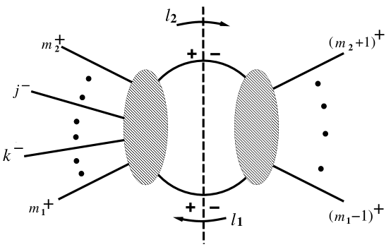
Figure 10: The possible intermediate helicities for a cut of a MHV amplitude, when both negative helicity gluons lie on the same side of the cut.

4.4 Example

As an example of how simple one-loop multi-parton cuts can be, we outline here the evaluation of the cuts for an infinite sequence of $n$-gluon amplitudes, the MHV amplitudes in $N=4$ super-Yang-Mills theory.$\!{}^{{\bf?}}$ We consider the single-trace, leading-color contribution $A_{n;1}$, and the case where the two negative helicity gluons lie on the same side of the cut, as shown in Fig. 10. (The case where they lie on the opposite side of the cut can be quickly reduced to this case $\!{}^{{\bf?}}$ using the SWI, Eqs. 76 and LABEL:eq:MHVSWI.) Contributions to this cut from intermediate fermions or scalars vanish using the “effective” supersymmetry of tree amplitudes, Eq. 76, plus conservation of fermion helicity and scalar particle number, on the right-hand side of the cut. The only contribution is from intermediate gluons with the helicity assignment shown in Fig. 10. The tree amplitudes on either side of the cut are pure-glue MHV tree amplitudes, so using Eq. 65 the cut takes the simple form

$$\int d{\rm LIPS}(-\ell_{1},\ell_{2})A^{\rm tree\ MHV}_{jk}(-\ell_{1},m_{1},\ldots,m_{2},\ell_{2})\hfill$$ (103)

$$\hskip 85.35826pt\times A^{\rm tree\ MHV}_{(-\ell_{2})\ell_{1}}(-\ell_{2},m_{2}+1,\ldots,m_{2}-1,\ell_{1})$$

$$= i\,A_{jk}^{\rm tree\ MHV}(1,2,\ldots,n)$$

$$\times\int d{\rm LIPS}(-\ell_{1},\ell_{2}){\left\langle m_{1}-1,\,m_{1}\right\rangle\left\langle\ell_{1}\,\ell_{2}\right\rangle\over\left\langle m_{1}-1,\,\ell_{1}\right\rangle\left\langle\ell_{1}\,m_{1}\right\rangle}\cdot{\left\langle m_{2},\,m_{2}+1\right\rangle\left\langle\ell_{2}\,\ell_{1}\right\rangle\over\left\langle m_{2}\,\ell_{2}\right\rangle\left\langle\ell_{2},\,m_{2}+1\right\rangle},$$

where the spinor products are labelled by either loop momenta ($\ell_{1},\ell_{2}$) or external particle labels, and the Lorentz-invariant phase space measure for the two-particle intermediate state is denoted by $d{\rm LIPS}(-\ell_{1},\ell_{2})$.

The integral in Eq. 103 can be viewed as a cut hexagon loop integral. (The four- and five-point cases are degenerate, since there are not enough external momenta to make a genuine hexagon.) To see this, use the on-shell condition $\ell_{1}^{2}=\ell_{2}^{2}=0$ to rewrite the four spinor product denominators in Eq. 103 as propagators multiplied by some numerator factor, for example

$${1\over\left\langle\ell_{1}\,m_{1}\right\rangle}={\left[m_{1}\,\ell_{1}\right]\over\left\langle\ell_{1}\,m_{1}\right\rangle\left[m_{1}\,\ell_{1}\right]}={\left[m_{1}\,\ell_{1}\right]\over 2\ell_{1}\cdot k_{m_{1}}}={-\left[m_{1}\,\ell_{1}\right]\over(\ell_{1}-k_{m_{1}})^{2}}\ .$$ (104)

In addition to these four propagators, there are two cut propagators implicit in $\int d{\rm LIPS}(-\ell_{1},\ell_{2})$.

Rather than evaluate the cut hexagon integral directly, we use the Schouten identity, Eq. 23, to reduce the number of spinor product factors in the denominator of each term, which will break up the integral into a sum of cut box integrals. We have

$${\left\langle m_{1}-1,\,m_{1}\right\rangle\left\langle\ell_{1}\,\ell_{2}\right\rangle\over\left\langle m_{1}-1,\,\ell_{1}\right\rangle\left\langle\ell_{1}\,m_{1}\right\rangle}={\left\langle m_{1}-1,\,\ell_{2}\right\rangle\over\left\langle m_{1}-1,\,\ell_{1}\right\rangle}-{\left\langle m_{1}\,\ell_{2}\right\rangle\over\left\langle m_{1}\,\ell_{1}\right\rangle}\ ,$$ (105)

and similarly for the second factor in Eq. 103. Four terms are generated, one of which is

$$\hskip-2.84526pt-i\,A_{jk}^{\rm tree\ MHV}(1,2,\ldots,n)\int d{\rm LIPS}(-\ell_{1},\ell_{2}){\left\langle m_{1}\,\ell_{2}\right\rangle\left[\ell_{2}\,m_{2}\right]\left\langle m_{2}\,\ell_{1}\right\rangle\left[\ell_{1}\,m_{1}\right]\over\left\langle m_{1}\,\ell_{1}\right\rangle\left[\ell_{1}\,m_{1}\right]\left\langle m_{2}\,\ell_{2}\right\rangle\left[\ell_{2}\,m_{2}\right]}\hfill$$

$$= \hskip-2.84526pt-i\,A_{jk}^{\rm tree\ MHV}(1,2,\ldots,n)\int d{\rm LIPS}(-\ell_{1},\ell_{2}){\mathop{\rm Tr}\nolimits\Bigl{(}\textstyle{1\over 2}(1+\gamma_{5})\not{\hbox{\kern-2.3pt$\ell$}}_{1}\not{\hbox{\kern-2.3pt$k$}}_{m_{1}}\not{\hbox{\kern-2.3pt$\ell$}}_{2}\not{\hbox{\kern-2.3pt$k$}}_{m_{2}}\Bigr{)}\over(\ell_{1}-k_{m_{1}})^{2}(\ell_{2}+k_{m_{2}})^{2}}\ .$$

This is the cut box integral $I_{4}^{m_{1},m_{2}}$, where the set of momenta flowing out of its four vertices is $\{k_{m_{1}},P_{m_{1}+1,m_{2}-1},k_{m_{2}},P_{m_{2}+1,m_{1}-1}\}$. The other three terms similarly give $I_{4}^{m_{1}-1,m_{2}}$, $I_{4}^{m_{1},m_{2}+1}$ and $I_{4}^{m_{1}-1,m_{2}+1}$, all with two loop momenta inserted in the numerator.

The $\gamma_{5}$-odd part of the trace in Eq. LABEL:eq:firstpartialfr does not contribute, because the box does not have enough independent momenta to satisfy the Levi-Civita tensor. The $\gamma_{5}$-even part can be reduced by standard Passarino-Veltman techniques $\!{}^{{\bf?}}$ to scalar box, triangle and bubble integrals. The coefficient of the scalar box integral $I_{4}^{m_{1},m_{2}}[1]$ is

$$-\textstyle{1\over 2}\bigl{(}P^{2}_{m_{1},m_{2}-1}P^{2}_{m_{1}+1,m_{2}}-P^{2}_{m_{1},m_{2}}P^{2}_{m_{1}+1,m_{2}-1}\bigr{)}\,.$$ (107)

After summing over the four box integrals, the triangles and bubbles cancel out. (This could have been anticipated from the exercise in Section 4.1, showing that $A^{N=4}$ exhibits loop-momentum cancellations down to $\ell^{m-4}$, plus the general loop integral reduction procedures discussed in Section 4.2.) Therefore the $N=4$ MHV amplitude which matches all the cuts is a sum of scalar box integrals, with coefficients given by Eq. 107, which evaluates explicitly (through ${\cal O}(\epsilon^{0})$) to

$$\hskip-11.38109ptA_{n;1}^{N=4}(1^{+},\ldots,j^{-},\ldots,k^{-},\ldots,n^{+})=(\mu^{2})^{\epsilon}\,c_{\Gamma}\,A_{jk}^{\rm tree\ MHV}(1,2,\ldots,n)\,V_{n}\,,$$ (108)

where the universal, cyclically symmetric function $V_{n}$ is given by

$$V_{2m+1} = \sum_{r=1}^{m-1}\sum_{i=1}^{n}f_{i,r}\ ,$$

$$V_{2m} = \sum_{r=1}^{m-2}\sum_{i=1}^{n}f_{i,r}+\sum_{i=1}^{n/2}f_{i,m-1}\ ,$$ (109)

with

$$\hskip-2.84526ptf_{i,r}\hskip-5.69054pt = \hskip-5.69054pt-{1\over\epsilon^{2}}\biggl{[}\bigl{(}-P^{2}_{i-1,i+r-1}\bigr{)}^{-\epsilon}+\bigl{(}-P^{2}_{i,i+r}\bigr{)}^{-\epsilon}-\bigl{(}-P^{2}_{i,i+r-1}\bigr{)}^{-\epsilon}-\bigl{(}-P^{2}_{i-1,i+r}\bigr{)}^{-\epsilon}\biggr{]}$$ (110)

$$+\mathop{\rm Li}\nolimits_{2}\biggl{(}1-{P^{2}_{i,i+r-1}\over P^{2}_{i-1,i+r-1}}\biggr{)}+\mathop{\rm Li}\nolimits_{2}\biggl{(}1-{P^{2}_{i,i+r-1}\over P^{2}_{i,i+r}}\biggr{)}$$

$$+\mathop{\rm Li}\nolimits_{2}\biggl{(}1-{P^{2}_{i-1,i+r}\over P^{2}_{i-1,i+r-1}}\biggr{)}+\mathop{\rm Li}\nolimits_{2}\biggl{(}1-{P^{2}_{i-1,i+r}\over P^{2}_{i,i+r}}\biggr{)}$$

$$-\mathop{\rm Li}\nolimits_{2}\biggl{(}1-{P^{2}_{i,i+r-1}P^{2}_{i-1,i+r}\over P^{2}_{i-1,i+r-1}P^{2}_{i,i+r}}\biggr{)}+{1\over 2}\ln^{2}\biggl{(}{P^{2}_{i-1,i+r-1}\over P^{2}_{i,i+r}}\biggr{)}\ .$$

The dilogarithm is defined by $\mathop{\rm Li}\nolimits_{2}(x)=-\int_{0}^{x}dt\ \ln(1-t)/t$, and by convention $(-P^{2}_{i-1,i-1})^{-\epsilon}=0^{-\epsilon}=0$.

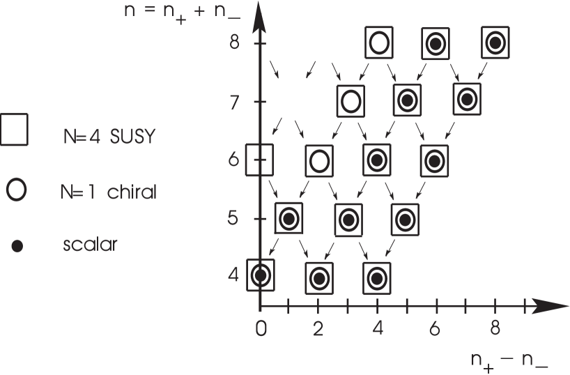
Figure 11: Currently known one-loop $n$-gluon amplitudes, decomposed into $N=4$ supersymmetric, $N=1$ chiral, and scalar contributions, as in Eq. 89. The number of external gluons with helicity $\pm 1$ in the amplitude is denoted by $n_{\pm}$. Parity reflects the figure about the vertical axis. Arrows show how amplitudes flow into each other under collinear limits.

It is remarkable that a compact expression for an infinite sequence of gauge theory loop amplitudes is so easy to obtain. Several other infinite sequences of $n$-gluon one-loop amplitudes have now been computed, using unitarity as well as collinear and recursive techniques.$\!{}^{{\bf?},{\bf?},{\bf?},{\bf?}}$ The currently known $n$-gluon amplitudes — or rather their components under the supersymmetric decomposition discussed in Section 4.1 — are plotted in Fig. 11 versus the number of helicity $\pm 1$ external states $n_{\pm}$. As the figure shows, the supersymmetric components are better known than the non-supersymmetric scalar terms. Polynomial ambiguities in the non-supersymmetric components of one-loop QCD amplitudes are the main obstacle to their efficient evaluation. In the various collinear limits, helicity amplitudes (including their polynomial terms) flow along the arrows in the figure, indicating how the limits may be used to help fix the ambiguities.

5 Conclusions

In these lectures we described techniques for efficient analytical calculation of scattering amplitudes in gauge theories, particularly QCD. Tools such as helicity and color decompositions, special gauges, unitarity, factorization limits and supersymmetric rearrangements can lead to many simplifications. Some of these ideas can be motivated from string theory, but none requires its detailed knowledge. There is no one “magic bullet” but rather a combined arsenal of techniques that work well together. At the practical level, some of these tools have been instrumental in calculating the one-loop five-parton amplitudes ($ggggg$, ${\bar{q}}q{\bar{q}}qg$ and ${\bar{q}}qggg$) which form the analytical bottleneck to NLO cross-sections for three-jet events at hadron colliders.$\!{}^{{\bf?},{\bf?},{\bf?}}$ They have also been used to obtain infinite sequences of special one-loop helicity amplitudes in closed form.$\!{}^{{\bf?},{\bf?},{\bf?},{\bf?}}$ On the other hand, many processes of experimental interest remain uncalculated at NLO and at higher orders, so there is plenty of room for improvement in the field!

References

References

- [1] CDF collaboration, Phys. Rev. Lett. 74:2626 (1995), Phys. Rev. D51:4623 (1995); D0 collaboration, Phys. Rev. Lett. 74:2632 (1995).
- [2] Z. Kunszt, in these proceedings.
- [3] M. Mangano and S. Parke, Phys. Rep. 200:301 (1991).
- [4] Z. Bern and D.A. Kosower, Phys. Rev. Lett. 66:1669 (1991); Z. Bern and D.A. Kosower, in Proceedings of the PASCOS-91 Symposium, eds. P. Nath and S. Reucroft (World Scientific, 1992); Z. Bern, Phys. Lett. 296B:85 (1992).
- [5] Z. Bern and D.A. Kosower, Nucl. Phys. B379:451 (1992).
- [6] F.A. Berends and W.T. Giele, Nucl. Phys. B294:700 (1987); M. Mangano, S. Parke and Z. Xu, Nucl. Phys. B298:653 (1988); M. Mangano, Nucl. Phys. B309:461 (1988).
- [7] Z. Bern and D.A. Kosower, Nucl. Phys. B362:389 (1991).
- [8] G. ’t Hooft, Nucl. Phys. B72:461 (1974); Nucl. Phys. B75:461 (1974); P. Cvitanović, Group Theory (Nordita, 1984).
- [9] Z. Bern, L. Dixon, D.C. Dunbar and D.A. Kosower, Nucl. Phys. B425:217 (1994).
- [10] Z. Bern, L. Dixon and D.A. Kosower, Nucl. Phys. B437:259 (1995).
- [11] F.A. Berends, R. Kleiss, P. De Causmaecker, R. Gastmans and T.T. Wu, Phys. Lett. B103:124 (1981); P. De Causmaeker, R. Gastmans, W. Troost and T.T. Wu, Nucl. Phys. B206:53 (1982); R. Kleiss and W.J. Stirling, Nucl. Phys. B262:235 (1985); R. Gastmans and T.T. Wu, The Ubiquitous Photon: Helicity Method for QED and QCD (Clarendon Press, 1990).
- [12] Z. Xu, D.-H. Zhang and L. Chang, Nucl. Phys. B291:392 (1987).
- [13] J.F. Gunion and Z. Kunszt, Phys. Lett. 161B:333 (1985).
- [14] S.J. Parke and T. Taylor, Phys. Lett. 157B:81 (1985); Z. Kunszt, Nucl. Phys. B271:333 (1986).
- [15] F.A. Berends and W.T. Giele, Nucl. Phys. B306:759 (1988).
- [16] D.A. Kosower, Nucl. Phys. B335:23 (1990).
- [17] S.J. Parke and T.R. Taylor, Phys. Rev. Lett. 56:2459 (1986).
- [18] Z. Kunszt and W.J. Stirling, Phys. Rev. D37:2439 (1988); C.J. Maxwell, Phys. Lett. B192:190 (1987).
- [19] M.T. Grisaru, H.N. Pendleton and P. van Nieuwenhuizen, Phys. Rev. D15:996 (1977); M.T. Grisaru and H.N. Pendleton, Nucl. Phys. B124:81 (1977).
- [20] F.A. Berends and W.T. Giele, Nucl. Phys. B313:595 (1989).
- [21] M. Mangano and S. J. Parke, Nucl. Phys. B299:673 (1988).
- [22] G. Altarelli and G. Parisi, Nucl. Phys. B126:298 (1977).
- [23] G. Sterman, in these proceedings.
- [24] A. Signer, Phys. Lett. B357:204 (1995).
- [25] A. Signer, Ph.D. Thesis, ETH-Zurich (1995).
- [26] R. Kleiss and W.J. Stirling, Nucl. Phys. B262:235 (1985); A. Ballestrero and E. Maina, Phys. Lett. B350:225 (1995); S. Dittmaier, Würzburg preprint 93-0023.
- [27] R. Vega and J. Wudka, preprint hep-ph/9511310.
- [28] Z. Bern, L. Dixon and D.A. Kosower, Phys. Rev. Lett. 70:2677 (1993).
- [29] G. ’t Hooft, in Acta Universitatis Wratislavensis no. 38, 12th Winter School of Theoretical Physics in Karpacz, Functional and Probabilistic Methods in Quantum Field Theory, Vol. 1 (1975) ; B.S. DeWitt, in Quantum gravity II, eds. C. Isham, R. Penrose and D. Sciama (Oxford, 1981); L.F. Abbott, Nucl. Phys. B185:189 (1981); L.F. Abbott, M.T. Grisaru and R.K. Schaefer, Nucl. Phys. B229:372 (1983).
- [30] W. Siegel, Phys. Lett. 84B:193 (1979); D.M. Capper, D.R.T. Jones and P. van Nieuwenhuizen, Nucl. Phys. B167:479 (1980); L.V. Avdeev and A.A. Vladimirov, Nucl. Phys. B219:262 (1983).
- [31] Z. Bern and D.C. Dunbar, Nucl. Phys. B379:562 (1992).
- [32] A.G. Morgan, Phys. Lett. B351:249 (1995).
- [33] Z. Bern, L. Dixon, D.C. Dunbar and D.A. Kosower, Nucl. Phys. B435:59 (1995).
- [34] J.L. Gervais and A. Neveu, Nucl. Phys. B46:381 (1972).
- [35] W. van Neerven and J. Vermaseren, Phys. Lett. 137B:241 (1984).
- [36] D.B. Melrose, Il Nuovo Cimento 40A:181 (1965).
- [37] Z. Bern, L. Dixon and D.A. Kosower, Phys. Lett. 302B:299 (1993); erratum ibid. 318:649 (1993).
- [38] Z. Bern, L. Dixon and D.A. Kosower, Nucl. Phys. B412:751 (1994).
- [39] L.M. Brown and R.P. Feynman, Phys. Rev. 85:231 (1952) ; G. Passarino and M. Veltman, Nucl. Phys. B160:151 (1979); G. ’t Hooft and M. Veltman, Nucl. Phys. B153:365 (1979).
- [40] G.J. van Oldenborgh and J.A.M. Vermaseren, Z. Phys. C46:425 (1990); G.J. van Oldenborgh, Ph.D. thesis, University of Amsterdam (1990).
- [41] Z. Bern, G. Chalmers, L. Dixon and D.A. Kosower, Phys. Rev. Lett. 72:2134 (1994).
- [42] Z. Bern and G. Chalmers, Nucl. Phys. B447:465 (1995).
- [43] L.D. Landau, Nucl. Phys. 13:181 (1959); S. Mandelstam, Phys. Rev. 112:1344 (1958), 115:1741 (1959); R.E. Cutkosky, J. Math. Phys. 1:429 (1960).
- [44] W.L. van Neerven, Nucl. Phys. B268:453 (1986); Z. Bern and A. Morgan, preprint hep-ph/11336; Z. Bern, L. Dixon and D.A. Kosower, to appear in Ann. Rev. Nucl. Part. Sci.
- [45] G.D. Mahlon, Phys. Rev. D49:2197 (1994); Phys. Rev. D49:4438 (1994).
- [46] Z. Kunszt, A. Signer and Z. Trócsányi, Phys. Lett. B336:529 (1994).