UFTP preprint 407/1996, TUM/T39-96-1

IR-Renormalon Contribution to the
Longitudinal Structure Function $F_{L}$

E. Stein^†, M. Meyer-Hermann^†, L. Mankiewicz^††, and A. Schäfer^†

^†Institut für Theoretische Physik, J. W. Goethe Universität Frankfurt,

Postfach 11 19 32, D-60054 Frankfurt am Main, Germany

^††Institut für Theoretische Physik, TU-München, D-85747 Garching, Germany

Abstract: The available data on $F_{L}$ suggest the existence of unexpected large higher twist contributions. We use the $1/N_{f}$ expansion to analyze the renormalon contribution to the coefficient function of the longitudinal structure function $F_{L}^{p-n}$. The renormalon ambiguity is calculated for all moments of the structure function thus allowing to estimate the contribution of “genuine” twist-4 corrections as a function of Bjorken-$x$. The predictions turn out to be in surprisingly good agreement with the experimental data.

One of the interesting quantities that can be measured in deep inelastic lepton-nucleon scattering is the ratio

$$R(x,Q^{2})=\frac{\sigma_{\rm L}(x,Q^{2})}{\sigma_{\rm T}(x,Q^{2})}=\frac{F_{2}(x,Q^{2})}{F_{2}(x,Q^{2})-F_{L}(x,Q^{2})}\left(1+\frac{4M^{2}x^{2}}{Q^{2}}\right)-1$$ (1)

of the total cross-sections for the scattering of longitudinally respectively transversely polarized photons and a nucleon, where $M$ is the nucleon mass and $F_{L}=F_{2}-2xF_{1}$. This ratio provides a clean test of the QCD interaction since it vanishes identically in the naive parton model. The experimental information on $R(x,Q^{2})$ is still limited [1], but much better data should be available in a few years from now. Phenomenological fits to the existing data [2] suggest surprisingly large higher-twist corrections of the form

$$R^{fit}(x,Q^{2})=\frac{b_{1}}{\ln(Q^{2}/\Lambda^{2})}\left(1+12\frac{Q^{2}}{Q^{2}+1}\,\frac{0.125^{2}}{0.125^{2}+x^{2}}\right)+\frac{b_{2}}{Q^{2}}+\frac{b_{3}}{Q^{4}+0.3^{2}}$$ (2)

where $\Lambda=0.2~{}\rm{GeV}$, $b_{1}=0.0635$, $b_{2}=0.5747$ and $b_{3}=-0.3534$ and all momenta are in GeV. So far the leading perturbative corrections and the target mass corrections to $R$ have been calculated [3]. The genuine power suppressed, i.e., $1/Q^{2}$ corrections can be analyzed in the framework of Operator Product Expansion [4, 5]. The power suppressed corrections which still have to be determined arise from matrix elements of higher twist operators and are sensitive to multiparton correlations within the target. An estimate of these matrix elements is a delicate problem which could not yet been solved.

By comparing the experimental data with the known corrections, it was possible however to disentangle mass corrections and true higher twist corrections [6] and even to estimate the magnitude of twist-4 matrix elements contributing to the second moment of the nucleon structure function $F_{L}$ and $F_{2}$ [7]

In the present paper we shall use the one-to-one correspondence between ultraviolet renormalons (UV) in the definition of higher twist corrections and infrared renormalons (IR) in the perturbative series which defines the twist-2 contribution to investigate the structure of power-suppressed corrections to the longitudinal structure function $F_{L}$.

IR-Renormalons have recently received much attention because of their potential to generate power-like corrections. For a physical quantity like $F_{L}$ the perturbative QCD series is not summable, even in the Borel sense, due to the appearance of fixed sign factorial growth of its coefficients. It results in a power-suppressed ambiguity of the magnitude $\sim\Lambda_{QCD}^{2}/Q^{2}$ [8]. Such terms show the need to include higher twist (non perturbative) corrections to give a meaning to a summed perturbation series [9, 10]. On the other hand also the higher twist corrections themselves are ill-defined. The ambiguity in their definition, due to the UV-renormalon, cancels exactly the IR-renormalon ambiguity in the perturbative series which describes the twist-2 term. In turn, the investigation of the ambiguities in the definition of the perturbation series of leading twist shows which higher twist corrections are needed for an unambiguous definition of a physical quantity.

In practice, one has observed the empirical fact that in cases where the perturbative series was studied in parallel with the higher twist corrections, such as the polarized Bjorken sum rule and the Gross Llewellyn-Smith sum rule, the ambiguities produced by IR renormalons in the leading twist contribution were roughly of the same order of magnitude as the best available theoretical estimates of the higher twist corrections [11]. Thus, despite fundamental objections [12], for phenomenological purposes one may use IR renormalons as a guide for the magnitude of higher-twist corrections [13]. The obvious advantage of such an approach is that the IR calculation can be done for all moments, and hence the result can be extended to the full $x$-dependence of the higher-twist contributions. One has to keep in mind, however, that the last step is even less justified, as the order of magnitude correspondence between IR ambiguities and higher twist corrections has been tested only for sum rules for first moments of structure functions.

We focus on the flavor non-singlet part of the longitudinal structure function

$$F_{L}^{p-n}(x,Q^{2})$$ (3)

i.e. on the difference between the proton and neutron structure function, and calculate the infrared renormalon contribution. This will also provide the exact coefficients of the perturbative series of $F_{L}$ in the large $N_{f}$ approximation [14, 15, 16]. In the framework of the ‘Naive Non Abelianization’ [17, 18, 19, 20] this can be used to approximate the non-leading $N_{f}$ terms.

We start with the well known hadronic scattering tensor of unpolarized deep inelastic lepton nucleon scattering parameterized in terms of two structure functions $F_{2}$ and $F_{L}$.

$$W_{\mu\nu}(p,q) = \frac{1}{2\pi}\,\int d^{4}ze^{iqz}\big{<}p\big{|}J_{\mu}(z)J_{\nu}(0)\big{|}p\big{>}$$

$$= \left({\rm g}_{\mu\nu}-\frac{q_{\mu}q_{\nu}}{q^{2}}\right)\frac{1}{2x}F_{L}(x,Q^{2})-\left({\rm g}_{\mu\nu}+p_{\mu}p_{\nu}\frac{q^{2}}{(p\cdot q)^{2}}-\frac{p_{\mu}q_{\nu}+p_{\nu}q_{\mu}}{p\cdot q}\right)\frac{1}{2x}F_{2}(x,Q^{2})$$

Here $J_{\mu}$ is the electromagnetic quark current, $x=Q^{2}/(2p\cdot q)$ and $q^{2}=-Q^{2}$. The nucleon state $\big{|}p\big{>}$ has momentum $p$ (averaging over the polarizations of the nucleon is understood). The non-singlet moments of the structure functions $F_{k}^{p-n}$ ($k=2,L$) can be expressed through operator product expansion [4] in the following form:

$$M_{k,N}(Q^{2}) = \int\limits_{0}^{1}dx\;x^{N-2}F_{k}^{p-n}(x,Q^{2})$$ (5)

$$= C_{k,N}\left(\frac{Q^{2}}{\mu^{2}},a_{s}\right)\left[A_{N}(\mu^{2})\right]^{p-n}+{\rm higher~{}twist}$$

where $a_{s}$ stands for

$$a_{s}=\frac{g^{2}}{16\pi^{2}}=\frac{\alpha_{s}}{4\pi}$$ (6)

and the $A_{N}$ are the spin-averaged matrix elements of the spin-N twist-2 operator

$$\big{<}p\big{|}\bar{\psi}\gamma^{\{\mu_{1}}iD^{\mu_{2}}\ldots iD^{\mu_{N}\}}\psi\big{|}p\big{>}^{p-n}=p^{\{\mu_{1}\ldots}p^{\mu_{N}\}}\left[A_{N}(\mu^{2})\right]^{p-n}$$ (7)

The inclusion of quark charges is implicitly understood. The flavors of the quark-operators $\psi$ are combined to yield the proton minus neutron matrix element. $\{\mu\nu\}$ indicates symmetric and traceless combinations. The higher twist corrections are given by matrix elements of twist-4 operators and were derived for the second moments of $F_{L}$ and $F_{2}$ in ref. [5].

$$p_{\{\mu}p_{\nu\}}\int\limits_{0}^{1}dx\;F_{L}^{p-n}(x,Q^{2}) = C_{L,2}\left(\frac{Q^{2}}{\mu^{2}},a_{s}\right)\big{<}p\big{|}\bar{\psi}\gamma_{\{\mu}iD_{\nu\}}\psi\big{|}p\big{>}^{p-n}$$ (8)

$$-\frac{C_{L,2}^{(a)}\left(Q^{2}/\mu^{2},a_{s}\right)}{4Q^{2}}\big{<}p\big{|}\bar{\psi}\left(D^{\alpha}gG_{\alpha\{\mu}\right)\gamma_{\nu\}}\psi\big{|}p\big{>}^{p-n}$$

$$-3\frac{C_{L,2}^{(b)}\left(Q^{2}/\mu^{2}),a_{s}\right)}{8Q^{2}}\big{<}p\big{|}\bar{\psi}\left\{g\tilde{G}_{\alpha\{\mu},iD_{\nu\}}\right\}_{+}\gamma^{\alpha}\gamma_{5}\psi\big{|}p\big{>}^{p-n}$$

where we used the conventions of [21]. In this equation we only retained the twist-4 corrections. The target mass corrections [22] are not explicitly shown. Due to the high dimension of the operators it is at present not possible to perform such a calculation reliably in the framework of lattice QCD or QCD sum rules. An additional problem of such a calculation is that a renormalization scheme has to be found in which quadratic divergences in twist-4 matrix elements do not produce mixing with lower dimension twist-2 operators. That is still an unsolved problem in lattice calculations [23, 24]. On the other hand, state of the art calculations of higher twist-corrections never claim an accuracy better than 30-50%. Therefore we claim that calculating the renormalon ambiguity in the coefficient function $C_{L,N}(Q^{2}/\mu^{2},a_{s})$ instead of the true higher-twist corrections to the longitudinal structure function is an legitimate procedure. The advantage is that such a calculation can be done for all $N$ therefore allowing to estimate the twist-4 corrections as a function of Bjorken-$x$. Note that a renormalon ambiguity in the coefficient function of the twist-2 spin-2 operator will only account for twist-4, spin-2, twist-6, spin-2 etc. operators and not for power suppressed twist-2 operators. This implies that target mass effects can not be traced by IR-renormalons.

The truncated perturbative expansion of the coefficient functions of the moments of $F_{L}$ and $F_{2}$ can be written as

$$C_{k,N}(1,a_{s})=\sum_{n=0}^{m_{0}(N)}B_{k,N}^{(n)}a_{s}^{n}+C_{k,N}^{(1)}\frac{\Lambda_{C}^{2}e^{-C}}{Q^{2}}+C_{k,N}^{(2)}\frac{\Lambda_{C}^{4}e^{-2C}}{Q^{4}}$$ (9)

where we have accounted for the asymptotic behaviour of the perturbation series which makes only sense up to a maximal order $m_{0}(N)$ depending on the magnitude of the expansion parameter $a_{s}$. With the standard normalization one finds $B_{L,N}^{(0)}=0$, $B_{2,N}^{(0)}=1$ and $B_{L,N}^{(1)}=4C_{F}/(1+N)$ [25]. $C_{F}=4/3$ is the eigenvalue of the Casimir operator of the $SU(3)$ colour group in the fundamental representation. We have indicated the ambiguity of the asymptotic expansion by including power suppressed terms. $\Lambda_{C}^{2}e^{-C}$ is a renormalization scheme independent quantity. $C=-5/3$ corresponds to $\Lambda_{\overline{MS}}$. We will show that only ambiguities up to order $1/Q^{4}$ will appear in the $1/N_{f}$ approximation for the longitudinal coefficient function. Since non-singlet $F_{L}$ and $F_{2}$ are to leading twist accuracy determined by the same operators we obtain from Eq. (5) with $Q^{2}=\mu^{2}$, $a_{s}=a_{s}(Q^{2})$

$$M_{L,N}(Q^{2})=\frac{\displaystyle\sum_{n=1}^{m_{0}(N)}B_{L,N}^{(n)}a_{s}^{n}+C_{L,N}^{(1)}\frac{\Lambda_{C}^{2}e^{-C}}{Q^{2}}}{\displaystyle 1+\sum_{n=1}^{m_{0}(N)}B_{2,N}^{(n)}a_{s}^{n}+C_{2,N}^{(1)}\frac{\Lambda_{C}^{2}e^{-C}}{Q^{2}}}\;M_{2,N}(Q^{2})$$ (10)

Expanding the denominator we find

$$M_{L,N}(Q^{2}) = \Big{[}B_{L,N}^{(1)}a_{s}+\left(B_{L,N}^{(2)}-B_{L,N}^{(1)}B_{2,N}^{(1)}\right)a_{s}^{2}+{\cal O}(a_{s}^{3})$$ (11)

$$+\frac{\Lambda_{C}^{2}e^{-C}}{Q^{2}}\left(C_{L,N}^{(1)}-\left(C_{L,N}^{(1)}B_{2,N}^{(1)}+C_{2,N}^{(1)}B_{L,N}^{(1)}\right)a_{s}+{\cal O}(a_{s}^{2})\right)\Big{]}M_{2,N}(Q^{2})$$

Since the Callan-Cross relation gives $B_{L,N}^{(0)}=0$ for all $N$ the calculation of the ambiguity in the perturbative expansion of $C_{L,N}$ alone is sufficient to determine power-suppressed contributions to $F_{L}^{p-n}(x,Q^{2})$ up to ${\cal O}(a_{s}/Q^{2})$ accuracy.

To extract the renormalon contribution to $C_{L,N}$ we calculate the coefficients to all orders in $a_{s}$ in the $1/N_{f}$ expansion where $N_{f}$ refers to the number of active flavours [14, 15, 16]. Each coefficient $B_{L,N}^{(m)}$ can be written as an expansion in $N_{f}$

$$B_{L,N}^{(m)}=B^{(m)}_{0}+B^{(m)}_{1}N_{f}+\ldots+B^{(m)}_{m}N_{f}^{m-1}$$ (12)

where the coefficient $B^{(m)}_{m}$ is unambiguously determined by the diagrams with one gluon-line that contains $m-1$ fermion bubble insertions. These diagrams can be calculated comparably easy while the non-leading terms are much harder to evaluate. The non-leading terms are approximated in the procedure of ”Naive Nonabelianization” (NNA) [19] where the highest power of $N_{f}$ is substituted by $N_{f}\to N_{f}-33/2=-\frac{3}{2}\beta_{0}$. Here

$$\beta_{0}=11-\frac{2}{3}N_{f}$$ (13)

is the one-loop coefficient of the QCD $\beta$-function. The exact coefficient is therefore approximated as

$$B_{L,N}^{(m)}\simeq B^{(m)}_{m}(N_{f}-\frac{33}{2})^{m-1}\;.$$ (14)

In cases where the exact higher order results are known, NNA approximates the exact coefficients well in the $\overline{MS}$-scheme [19]. In what follows we are going to calculate the coefficients $B_{L,N}^{(m)}$ of the $(\beta_{0}a_{s})^{m-1}$ expansion. For that we split the exact coefficient into

$$B_{L,N}^{(m+1)}=\tilde{B}_{L,N}^{(m)}+\delta_{L,N}^{(m)}\;.$$ (15)

While $\tilde{B}_{L,N}^{(m)}$ contains only the effects of one-loop running of the coupling to order $m$, only $\delta_{L,N}^{(m)}$ requires a true $m$-loop calculation. It will be checked a posteriori by comparison with those coefficient that are known exactly whether the neglection of $\delta_{L,N}^{(m)}$ is justified (see Eq. (S0.Ex10) and Table (1)). Note that $B_{L,N}^{(1)}=\tilde{B}_{L,N}^{(0)}=4C_{F}/(N+1)$. In the following the NNA approximation to the coefficient function $C_{L,N}(a_{s})$ will be written as $\tilde{C}_{L,N}(a_{s})$.

A convenient way to calculate $\tilde{C}_{L,N}(a_{s})$ is to deal with its Borel transform

$$BT[\tilde{C}_{L,N}(a_{s})](s)=\sum_{m=0}s^{m}\beta_{0}^{-m}\frac{\tilde{B}_{L,N}^{(m)}}{m!}\;.$$ (16)

The advantage of that representation is manifold. The Borel transform can be used as generating function for the fixed order coefficients

$$\tilde{B}_{L,N}^{(m)}=\left.\beta_{0}^{m}\frac{d^{m}}{ds^{m}}BT[\tilde{C}_{L,N}(a_{s})](s)\right|_{s=0}$$ (17)

and the sum of all diagrams can be defined by the integral representation

$$\tilde{C}_{L,N}(a_{s})=\frac{1}{\beta_{0}}\int\limits_{0}^{\infty}ds\,e^{-s/(\beta_{0}a_{s})}BT[\tilde{C}_{L,N}(a_{s})](s)\;.$$ (18)

Technically the most important point is the simplification of the calculation of the Borel transform of diagrams with only one fermion bubble chain. In that case the Borel transform can be applied directly to the effective gluon propagator which resums the fermion bubble chain. The effective (Borel-transformed) gluon propagator is [26]

$$BT[a_{s}D^{AB}(k)](s)=i\delta^{AB}\frac{k_{\mu}k_{\nu}-k^{2}{\rm g}_{\mu\nu}}{(-k^{2})^{2}}\left(\frac{\mu^{2}e^{-C}}{-k^{2}}\right)^{s}\;.$$ (19)

In fact one only has to calculate the leading-order diagram with the usual gluon propagator substituted by the above one in which only the usual denominator of $(-k^{2})^{-2}$ is changed to $(-k^{2})^{-(2+s)}$.

To obtain the coefficient function $\tilde{C}_{L,N}(1,a_{s})$ we have to calculate the ${\cal O}(a_{s})$ correction to the Compton forward scattering amplitude with the effective propagator Eq. (19). We get

$$BT[\tilde{C}_{L,N}(a_{s})](s) = C_{F}\left(\frac{\mu^{2}e^{-C}}{Q^{2}}\right)^{s}\frac{8}{(2-s)(1-s)(1+s+N)}\frac{\Gamma(s+N)}{\Gamma(1+s)\Gamma(N)}$$

$$= C_{F}\left(\frac{\mu^{2}e^{-C}}{Q^{2}}\right)^{s}8\frac{\Gamma(s+N)}{\Gamma(1+s)\Gamma(N)}$$

$$\times\left(\frac{1}{(2+N)(1-s)}-\frac{1}{(3+N)(2-s)}+\frac{1}{(2+N)(3+N)(1+s+N)}\right)\,.$$

The Borel transform exhibits IR-renormalons at $s=1$ and $s=2$. The position of the UV-renormalon $s=-1-N$ depends on the moment $N$ one is dealing with. Formula Eq. (S0.Ex9) has been derived independently in [27].

The NNA approximants to the coefficient function in all orders in $a_{s}$ can be derived setting $\mu^{2}=Q^{2}$ and $C=-5/3$ in equation Eq. (S0.Ex9). It is interesting to compare the approximation of the NNA procedure with the exact results derived by Larin et al. [28] for the non singlet moments $N=2,~{}4,~{}6,~{}8$, denoted by $C_{L,N}$.

$$\tilde{C}_{L,2}(1,a_{s}) = a_{s}\cdot 1.77778+a_{s}^{2}(74.963-4.54321N_{f})+a_{s}^{3}(3238.62-392.56N_{f}+11.8957N_{f}^{2})$$

$$C_{L,2}(1,a_{s}) = a_{s}\cdot 1.77778+a_{s}^{2}(56.755-4.54321N_{f})+a_{s}^{3}\Big{(}2544.60-421.69N_{f}+11.8957N_{f}^{2}$$

$$-23.21\sum_{f=1}^{N_{f}}q_{f}\Big{)}$$

$$\tilde{C}_{L,4}(1,a_{s}) = a_{s}\cdot 1.06667+a_{s}^{2}(56.32-3.41333N_{f})+a_{s}^{3}(2964.52-359.336N_{f}+10.889N_{f}^{2})$$

$$C_{L,4}(1,a_{s}) = a_{s}\cdot 1.06667+a_{s}^{2}(47.99-3.41333N_{f})+a_{s}^{3}\Big{(}2523.74-383.052N_{f}+10.889N_{f}^{2}$$

$$-15.18\sum_{f=1}^{N_{f}}q_{f}\Big{)}$$

$$\tilde{C}_{L,6}(1,a_{s}) = a_{s}\cdot 0.761905+a_{s}(44.4789-2.69569N_{f})+a_{s}^{2}(2578.8-312.582N_{f}+9.47219N_{f}^{2})$$

$$C_{L,6}(1,a_{s}) = a_{s}\cdot 0.761905+a_{s}(40.9962-2.69569N_{f})+a_{s}^{2}\Big{(}2368.2-340.069N_{f}+9.47219N_{f}^{2}$$

$$-11.12\sum_{f=1}^{N_{f}}q_{f}\Big{)}$$

$$\tilde{C}_{L,8}(1,a_{s}) = a_{s}\cdot 0.592593+a_{s}^{2}(36.8193-2.23147N_{f})+a_{s}^{2}(2269.79-275.126N_{f}+8.33715N_{f}^{2})$$

$$C_{L,8}(1,a_{s}) = a_{s}\cdot 0.592593+a_{s}^{2}(35.8766-2.23147N_{f})+a_{s}^{2}\Big{(}2215.21-305.473N_{f}+8.33715N_{f}^{2}$$ (21)

$$-8.74\sum_{f=1}^{N_{f}}q_{f}\Big{)}$$

		Exact results [28]	NNA approximants
$N=2$	$N_{F}=3$	$43.1254\;a_{s}^{2}+1386.59\;a_{s}^{3}$	$61.3333\;a_{s}^{2}+2168.\;a_{s}^{3}$
	$N_{F}=4$	$38.5822\;a_{s}^{2}+1032.7\;a_{s}^{3}$	$56.7901\;a_{s}^{2}+1858.71\;a_{s}^{3}$
$N=4$	$N_{F}=3$	$37.75\;a_{s}^{2}+1472.58\;a_{s}^{3}$	$46.08\;a_{s}^{2}+1984.51\;a_{s}^{3}$
	$N_{F}=4$	$34.3367\;a_{s}^{2}+1155.64\;a_{s}^{3}$	$42.6667\;a_{s}^{2}+1701.4\;a_{s}^{3}$
$N=6$	$N_{F}=3$	$32.9091\;a_{s}^{2}+1433.24\;a_{s}^{3}$	$36.3918\;a_{s}^{2}+1726.31\;a_{s}^{3}$
	$N_{F}=4$	$30.2134\;a_{s}^{2}+1152.07\;a_{s}^{3}$	$33.6961\;a_{s}^{2}+1480.03\;a_{s}^{3}$
$N=8$	$N_{F}=3$	$29.1822\;a_{s}^{2}+1373.83\;a_{s}^{3}$	$30.1249\;a_{s}^{2}+1519.45\;a_{s}^{3}$
	$N_{F}=4$	$26.9507\;a_{s}^{2}+1117.97\;a_{s}^{3}$	$27.8934\;a_{s}^{2}+1302.68\;a_{s}^{3}$

Table 1: Comparison of the NNA approximants to the exact results obtained in [28] for the coefficient function $C_{L,N}(1,a_{s})$ up to order ${\cal O}(a_{s}^{3})$. We have omitted the ${\cal O}(a_{s})$ corrections which agree exactly.

		Exact results [29]	NNA approximants
$N=2$	$N_{F}=3$	$1.69381\;a_{s}^{2}$	$71.9999\;a_{s}^{2}$
	$N_{F}=4$	$-3.63952\;a_{s}^{2}$	$66.6666\;a_{s}^{2}$
$N=4$	$N_{F}=3$	$91.3793\;a_{s}^{2}$	$229.3403\;a_{s}^{2}$
	$N_{F}=4$	$74.3914\;a_{s}^{2}$	$212.3488\;a_{s}^{2}$
$N=6$	$N_{F}=3$	$218.3608\;a_{s}^{2}$	$378.1762\;a_{s}^{2}$
	$N_{F}=4$	$190.3477\;a_{s}^{2}$	$350.1631\;a_{s}^{2}$
$N=8$	$N_{F}=3$	$357.0326\;a_{s}^{2}$	$511.9848\;a_{s}^{2}$
	$N_{F}=4$	$319.1078\;a_{s}^{2}$	$474.06\;a_{s}^{2}$
$N=10$	$N_{F}=3$	$498.6271\;a_{s}^{2}$	$632.6276\;a_{s}^{2}$
	$N_{F}=4$	$451.7658\;a_{s}^{2}$	$585.7663\;a_{s}^{2}$

Table 2: Same as Table 1 for the coefficient function $C_{2,N}(1,a_{s})$ of the moments of the structure function $F_{2}^{p-n}$. These were obtained in [29] up to order ${\cal O}(a_{s}^{2})$. On the right column we compare these with the NNA approximants. The ${\cal O}(a_{s})$ corrections agree exactly.

The sum over the quark charges $\sum_{f=1}^{N_{f}}q_{f}$ stems from the exact calculation of the so called light-by-light diagrams where the photon vertices are connected with different fermion lines. Those diagrams first appear at three-loop level.

The subleading $N_{f}$ coefficients approximate those of the exact expression in sign and magnitude. The leading $N_{f}a_{s}^{2}$ and $N_{f}^{2}a_{s}^{3}$ coefficients of course agree exactly. The numerically important cases $N_{f}=3$ and $N_{f}=4$ are given in table 1. For comparison we have also given the NNA approximants to the exact ${\cal O}(a_{s})$ corrections to the coefficient function of the structure function $F_{2}$ that were calculated in [29]. It is interesting to observe that NNA approximates the higher moments consistently better than the lower ones and gives better results for $F_{L}$ than for $F_{2}$. These features can be understood as follows. The most problematic property of NNA is the neglect of multiple gluon emission. As such processes are important for small $x$ we cannot expect our NNA structure functions to be correct in this region. Ever higher moments of the structure functions are less and less sensitive to their small-$x$ behaviour and therefore the NNA should systematically improve.

As can be seen from Eq. (S0.Ex9) the perturbative expansion of $\tilde{C}_{L,N}$ is not Borel summable. The poles in the Borel representation at $s=1$ and $s=2$ destroy a reconstruction of the summed series via Eq. (18). Asymptotically the first IR-Renormalon, i.e. the pole at $s=1$ will dominate the perturbative expansion giving rise to a factorial growth of the coefficient

$$\lim_{m\to\infty}\tilde{B}_{L,N}^{(m)}\sim\left.\beta_{0}^{m}\frac{d^{m}}{ds^{m}}\frac{1}{1-s}\right|_{s=0}=\beta_{0}^{m}m!$$ (22)

This means that a perturbative expansion at best can be regarded as an asymptotic expansion and the expansion makes sense only up to a maximal value $m=m_{0}\sim\log(Q^{2}/\Lambda^{2})$. For higher values of $m>m_{0}$ the fixed order contributions will increase and finally diverge. The general uncertainty in the perturbative prediction is then of the order of the minimal term in the expansion. It can be estimated either directly or by taking the imaginary part $\Im/\pi$ (divided by $\pi$) of the Borel transform [11]. From Eq. (18) we get for the function Eq. (S0.Ex9)

$$\frac{\Im}{\pi}\frac{1}{\beta_{0}}\int\limits_{0}^{\infty}ds\,e^{-s/(\beta_{0}a_{s})}BT[\tilde{C}_{L,N}(a_{s})](s)=\pm\frac{8C_{F}}{\beta_{0}}\frac{\Lambda_{C}^{2}e^{-C}}{Q^{2}}\frac{N}{N+2}\pm\frac{4C_{F}}{\beta_{0}}\frac{\Lambda_{C}^{4}e^{-2C}}{Q^{4}}\frac{N^{2}+N}{N+3}$$ (23)

The ambiguity in the sign of the IR-renormalon contributions is due to the two possible contour deformations above or below the pole at $s=1$ and $s=2$. For the moments of $F_{L}^{p-n}$ we then get

$$M_{L,N}(Q^{2})=\Bigg{[}C_{F}\frac{4}{1+N}a_{s}+{\cal O}(a_{s}^{2})\pm\left(\frac{8C_{F}}{\beta_{0}}\frac{N}{N+2}+{\cal O}(a_{s})\right)\frac{\Lambda_{\overline{MS}}^{2}e^{5/3}}{Q^{2}}\Bigg{]}M_{2,N}(Q^{2})$$

Observing that

$$\int\limits_{0}^{1}dx\;x^{N-2}\left(\delta(x-1)-2x^{3}\right) = \frac{N}{N+2}$$ (25)

the above equation is easily transformed from the moment-space to Bjorken-$x$ space.

$$F_{L}^{p-n}(x,Q^{2})+\frac{4x^{2}M^{2}}{Q^{2}}F_{2}^{p-n}(x,Q^{2})=4C_{F}a_{s}(Q^{2})\int\limits_{x}^{1}\frac{dy}{y}\left(\frac{x}{y}\right)^{2}F_{2}^{p-n}(y,Q^{2})+{\cal O}(a_{s}^{2})$$

$$\hskip 62.59605pt\pm\frac{8C_{F}}{\beta_{0}}\frac{\Lambda_{\overline{MS}}^{2}e^{5/3}}{Q^{2}}\left[F_{2}^{p-n}(x,Q^{2})-2\int\limits_{x}^{1}\frac{dy}{y}\left(\frac{x}{y}\right)^{3}F_{2}^{p-n}(y,Q^{2})+{\cal O}(a_{s})\right]$$

$$\hskip 62.59605pt+4x^{3}\frac{M^{2}}{Q^{2}}\int\limits_{x}^{1}\frac{dy}{y}F^{p-n}_{2}(y,Q^{2})$$ (26)

We have neglected the contribution of the second IR-renormalon since it is of the order of $1/(Q^{2})^{2}$ while there is a contribution of order $a_{s}/Q^{2}$ related to the ambiguity in the coefficient function of $F_{2}$ which we have not included. We have included the kinematical and target mass corrections to the order we are working as given in [6].

In connection to the IR renormalon, it is interesting to investigate the corresponding ambiguity in the definition of the twist-4 matrix elements. This can be done for the second moment of $F_{L}$ where the contributing twist-4 operators are known, see Eq. (8). Composite operators have to be renormalized individually and have their own renormalization scale dependence. Operators of a higher twist, and therefore of a higher dimension, exhibit power-like UV divergences in addition to the usual logarithmic ones. In particular, a quadratic divergence of a twist-4 matrix element contributing to $F_{L}$, results in a mixing with the lower-dimension twist-2 matrix element. When the calculation of the matrix element is done in the framework of dimensional regularization, the quadratic divergence does not appear explicitely. It manifests itself as $\Gamma(1-d/2)$ factor, singular at $d=4$, and at $d=2$, where it corresponds to usual logarithmic divergence. Evaluating the one loop contribution to the quark matrix elements of twist-4 operators, with the Borel transformed propagator (Eq. (19)), in $d=4$ dimensions we obtain an expression singular at $s=1$.

$$\left.BT\left[\tilde{C}_{L,2}^{(a)}(a_{s})\big{<}p\big{|}\bar{\psi}\left(D^{\alpha}gG_{\alpha\{\mu}\right)\gamma_{\nu\}}\psi\big{|}p\big{>}^{p-n}\right](s)\right|_{s\to 1} = \frac{2C_{F}}{1-s}\left(\frac{\mu^{2}e^{-C}}{Q^{2}}\right)\big{<}p\big{|}\bar{\psi}\gamma_{\{\mu}iD_{\nu\}}\psi\big{|}p\big{>}^{p-n}$$

$$\left.BT\left[\tilde{C}_{L,2}^{(b)}(a_{s})\big{<}p\big{|}\bar{\psi}\left\{g\tilde{G}_{\alpha\{\mu},iD_{\nu\}}\right\}_{+}\gamma^{\alpha}\gamma_{5}\psi\big{|}p\big{>}^{p-n}\right](s)\right|_{s\to 1} = \frac{28}{3}\frac{C_{F}}{1-s}\left(\frac{\mu^{2}e^{-C}}{Q^{2}}\right)\big{<}p\big{|}\bar{\psi}\gamma_{\{\mu}iD_{\nu\}}\psi\big{|}p\big{>}^{p-n}$$

The singularities at $s=1$ is the manifestation of quadratic UV divergences. Inserting this together with Eq. (S0.Ex9) into the operator product expansion for the second moment of $F_{L}$ we see that this contribution indeed cancels against the IR-renormalon contribution to the coefficient function of the twist-2 term, resulting in an expression which is free of perturbatively generated ambiguities up to the $\Lambda^{2}/Q^{2}$ order.

The appearance of an IR-renormalon ambiguity in a perturbative calculation thus indicates the need to include higher twist corrections to interpret the perturbative expansion to all orders. Of course one can argue that the numerical value of the IR-renormalon uncertainty has no physical significance since it has to cancel in a complete calculation. As we explained above, in some case a higher twist estimate based on IR renormalon ambiguity has proven to be a fairly good guess, at least for low moments of the structure functions. In the present case the IR calculation can be easily done for all moments, so that the result can be extended to produce a model of the the full $x$-dependence of higher twist effects. We keep in mind that such a model cannot have significance beyond phenomenological level for the following reason. The renormalons ambiguity in the coefficient function $C_{L,N}(Q^{2})$ is a target independent quantity of pure perturbative nature, while “genuine” higher twist matrix elements are a measure of multiparticle correlations in the target and are process dependent.

It is interesting to compare our prediction for the twist-4 part of $F_{L}$ with the available experimental data. To this end we use the phenomenological parametrizations for $R(x,Q^{2})$ Eq. (2) of [2]. To extract $F_{L}(x,Q^{2})$ we have choosen the parametrization of $F_{2}^{p}(x,Q^{2})$ and $F_{2}^{d}(x,Q^{2})$ of [30] valid in the region $0.006<x<0.9$ and $0.5<Q^{2}<75~{}{\rm GeV^{2}}$. With $F_{2}^{p-n}\simeq 2(F_{2}^{p}-F_{2}^{d})$ we have

$$F_{L}+\frac{4M^{2}x^{2}}{Q^{2}}F_{2}=\frac{R}{R+1}\left(1+\frac{4M^{2}x^{2}}{Q^{2}}\right)F_{2}\\ =F_{L}^{\rm twist-2}(x,Q^{2})+\frac{d^{\rm fit}(x,Q^{2})}{Q^{2}}+{\cal O}\left(\frac{1}{Q^{4}}\right)\,,$$

where we neglect the ${\cal O}(1/Q^{4})$ contributions for consistent comparison with our calculation. The $Q^{2}$ dependence of the higher twist coefficient $d^{\rm fit}(x,Q^{2})$ is only logarithmic. In Figure 1 we compare the experimental fit of the higher-twist coefficient with the QCD-calculation (Eq. (S0.Ex22)), where we have shown target mass and twist-4 contributions separately. We observe a rather large contribution coming from the IR renormalon estimate for the twist-4 part, which accounts for more than half of the discrepancy between the experimental fit and a prediction which takes into account the target mass correction only. The sign of the IR renormalon contribution, which cannot be determined theoretically, should be choosen positive. This leads to an astonishing agreement (possible somewhat fortuitous) with the experimental fit. Our estimate based on the calculation of the IR ambiguity has proven to be phenomenologically surprisingly successful, predicting a high twist-4 contribution to $F_{L}$ in accordance with experimental results. It further supports the idea that, while the rigorous QCD calculations of higher twist contribution to $F_{L}$ are not yet available, calculations like the one presented in this paper can be used to predict the order of magnitude of power suppressed corrections.

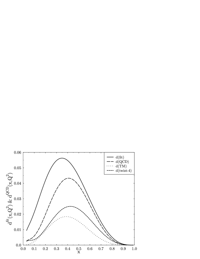
Figure 1: Comparison of $d^{QCD}(x,Q^{2})$ (long dashed line), the power suppressed contribution on the right hand side of Eq. (S0.Ex22), with the phenomenological fit $d^{\rm fit}(x,Q^{2})$ (full line) Eq. (S0.Ex26). We have also plotted the IR-renormalon (twist-4) part (short dashed line) and the target mass corrections (dotted line) separately. The agreement with experiment is much better including twist-4 corrections than without them (dotted line). We have chosen $\Lambda_{\overline{MS}}=250~{}{\rm MeV}$, $Q^{2}=5~{}{\rm GeV}$ and $N_{f}=4$.

Acknowledgements. This work has been supported by BMBF and DFG (G.Hess Programm). A.S. thanks also the MPI für Kernphysik in Heidelberg for support.

References

• [1] S. Dasu et al., Phys.Rev.Lett. 61, 1061 (1988)
• [2] L.W. Whitlow, S. Rock, A. Bodek, S. Dasu, and E.M. Riordan, Phys. Lett.  B250, 193 (1990)
• [3] G. Altarelli and G. Martinelli, Phys.Lett. B76, 89, (1978)
E.B. Zijlstra and W.L. van Neerven, Nucl.Phys. B383, 525 (1992)
• [4] H.D. Politzer, Phys.Rev.Lett. 30, 1346 (1973)
D.J. Gross and F. Wilczek, Phys.Rev.Lett. 30, 1323 (1973)
• [5] E.V. Shuryak and A.I. Vainshtein, Nucl.Phys. B199, 451, (1982)
R.L. Jaffe and M. Soldate, Phys.Rev. D26, 49 (1982)
• [6] J. Sanchez Guillen, J.L. Miramontes, M. Miramontes, G. Parente, and O.A. Sampayo, Nucl. Phys. B353, 337 (1991)
• [7] S. Choi, T. Hatsuda, Y. Koike, and Su H. Lee, Phys. Lett. B312 351 (1993)
• [8] A.H. Mueller, The QCD perturbation series., in “QCD - Twenty Years Later”, edited by P.M. Zerwas and H.A. Kastrup, 162, (World Scientific 1992)
• [9] V. I. Zakharov, Nucl. Phys.  B385, 452 (1992)
• [10] A.H. Mueller, Phys. Lett.  B 308, 355 (1993)
• [11] V. M. Braun, QCD renormalons and higher twist effects. hep-ph/9505317 (1995)
• [12] Yu. L. Dokshitzer and N. G. Uraltsev, Are IR renormalons a good probe for the strong interaction domain? hep-ph/9512407 (1995)
Yu. L. Dokshitzer, G. Marchesini and B.R. Webber, Dispersive approach to power-behaved contributions in QCD hard processes, hep-ph/9512336 (1995)
• [13] M. Beneke and V.M. Braun, Nucl. Phys. B454, 253 (1995)
• [14] D.J.Broadhurst, Z.Phys. C58, 339 (1993)
• [15] D.J.Broadhurst and A.L. Kataev, Phys.Lett. B315, 179 (1993)
• [16] C.N. Lovett-Turner, C.J. Maxwell, Nucl. Phys.  B452 188 (1995)
• [17] D.J.Broadhurst and A.G.Grozin, Phys.Rev.D 52, 4082 (1995)
• [18] M. Beneke and V.M. Braun, Phys.Lett. B348, 513 (1995)
• [19] P. Ball, M. Beneke and V.M. Braun, Nucl. Phys. B452, 563 (1995)
• [20] M. Neubert, Nucl. Phys.  B405, 424 (1995)
• [21] T. Muta, Foundations of Quantum Chromodynamics, World Scientific 1987
• [22] H. Georgi and H.D. Politzer, Phys. Rev. D14, 1829 (1976)
• [23] X. Ji, Nucl.Phys. B448 51 (1995)
• [24] G. Martinelli, C.T. Sachrajda, Phys. Lett. B354 423 (1995)
• [25] W.A. Bardeen, A.J. Buras, D.W. Duke, and T. Muta, Phys. Rev. D18, 3998 (1978)
• [26] M. Beneke Nucl.Phys. B405 424 (1993)
• [27] J.A. Gracey, Large $N_{f}$ methods for computing the perturbative structure of deep inelastic scattering. hep-ph/9509276, LTH-346
• [28] S.A. Larin, T. van Ritbergen, J.A.M. Vermaseren, Nucl.Phys. B427, 41 (1994)
• [29] S.A. Larin and J.A.M. Vermaseren, Z.Phys. C57, 93 (1993)
• [30] NMC, M. Arneodo et al., Measurement of the proton and the deuteron structure functions $F_{2}^{p}$ and $F_{2}^{d}$, CERN-PPE/95-138, hep-ph/9509406