NORDITA-96/3 P

hep-ph/9601333

January 25, 1996

Charmonium Production via Fragmentation

at Higher Orders in $\alpha_{s}$
P. Ernström, P. Hoyer, and M. Vänttinen
NORDITA

Blegdamsvej 17, DK-2100 Copenhagen Ø

Quarkonium production at a given large $p_{T}$ is dominated by parton fragmentation: a parton which is produced with transverse momentum $p_{T}/z$ fragments into a quarkonium state which carries a fraction $z$ of the parton momentum. Since parton production cross sections fall steeply with $p_{T}$, high $z$ fragmentation is favored. However, quantum number constraints may require the emission of gluons in the fragmentation process, and this softens the $z$ dependence of the fragmentation function. We discuss the possibility that higher-order processes may enhance the large $z$ part of fragmentation functions and thus contribute significantly to the quarkonium cross section. An explicit calculation of light quark fragmentation into $\eta_{c}$ shows that the higher-order process $q\rightarrow q\eta_{c}$ in fact dominates the lowest-order process $q\rightarrow qg\eta_{c}$.

1. Introduction

Heavy quark production is a hard QCD process, and the perturbative expansion of production amplitudes in $\alpha_{s}$ is expected to apply. However, the perturbation series is not always dominated by its lowest-order term. For example, when the transverse momentum $p_{T}$ of a collinear heavy quark pair is much larger than its invariant mass $M$, light parton fragmentation dominates the lowest-order production processes by a power of $p_{T}^{2}/M^{2}$ [1]. The data on charmonium production indeed shows a $1/p_{T}^{4}$ behavior of the cross section [2, 3], compatible with the prediction for a fragmentation process.

QCD calculations based on the color singlet model [4] nevertheless disagree with data on the relative production rates of $S$ and $P$ wave quarkonia and on the absolute normalization of the cross sections at both low [5, 6] and high [2, 3, 7] values of $p_{T}$. Order-of-magnitude discrepancies have been observed for both charmonium and bottomonium.

In QCD, the fragmentation of a virtual gluon into a ${}^{3}S_{1}$ quarkonium state ($J/\psi,\ \Upsilon$) requires the emission of at least two extra gluons, $g^{*}\rightarrow\mbox{}^{3}S_{1}+gg$, whereas fragmentation into a ${}^{3}P_{J}$ state can proceed with the emission of a single gluon, $g^{*}\rightarrow\mbox{}^{3}P_{J}+g$. The emission of the extra gluon suppresses the calculated ${}^{3}S_{1}$ cross section considerably compared to the ${}^{3}P_{J}$ cross section, due to the extra power of $\alpha_{s}$ and also because the emitted gluons carry away part of the transverse momentum of the fragmenting gluon. The experimental ${}^{3}S_{1}$/${}^{3}P_{2}$ cross section ratio is much larger than the calculated one.

The discrepancy could be related to the bound state dynamics of the quarkonia. This is the solution proposed by the color octet model [8, 9]. The gluon is assumed to first fragment into a $Q\bar{Q}$ pair in a color octet state. Later, after a formation time characteristic of the bound state, the pair couples to the physical quarkonium through the absorption or emission of one or two soft gluons. The momenta of the emitted gluons are typical of the quarkonium bound state dynamics, and thus they carry away only a minor part of the transverse momentum.

Although the probabilities of these nonperturbative transitions are essentially free parameters, the octet model makes specific predictions about the polarization of the produced quarkonium [10]. The ${}^{3}S_{1}$ quarkonia produced by the fragmentation of a nearly real gluon are expected to be transversely polarized. The data to test this prediction is not yet available. Note that theoretical calculations of quarkonium polarization can be compared with data in fixed-target experiments. In this case, neither the color singlet model nor the color octet model can explain the experimentally observed unpolarized production [6, 11].

Here we wish to draw attention to the possibility that higher-order perturbative contributions to fragmentation mechanisms could be enhanced by the so-called trigger bias effect. When the transverse momentum $p_{T}$ of the quarkonium is fixed, processes which allow the fragmenting parton to be produced with the lowest possible transverse momentum $p_{T}/z$ are favored. The large $p_{T}$ cross section is a convolution of the production cross section $\sigma_{i}$ of a parton $i$ and its fragmentation function $D_{i\rightarrow{\cal O}}$ to the quarkonium state ${\cal O}$,

$${d\sigma_{\cal O}(s,p_{T})\over dp_{T}}=\sum_{i}\int_{0}^{1}dz{d\sigma_{i}\over d{p_{i}}_{T}}(s,p_{T}/z,\mu)D_{i\rightarrow{\cal O}}(z,\mu),$$ (1)

where $\mu$ is the factorization scale. The parton production cross section $d\sigma_{i}/d{p_{i}}_{T}$ falls approximately as $(p_{T}/z)^{-4}$, which implies the enhancement of high $z$ fragmentation by a factor $z^{4}$. As a rough measure of the importance of a fragmentation function ${D}_{i\rightarrow{\cal O}}(z,\mu)$ we can therefore use its fifth moment ${D}^{(5)}_{i\rightarrow{\cal O}}(\mu)$, defined by

$${D}^{(n)}_{i\rightarrow{\cal O}}(\mu)\equiv\int_{0}^{1}dzz^{n-1}D_{i\rightarrow{\cal O}}(z,\mu).$$ (2)

We have studied the importance of higher-order fragmentation contributions in the case of light quark fragmention into ${}^{1}S_{0}$ quarkonium ($\eta_{c}$) within the color singlet model. The relevant Feynman diagrams are shown in Fig. 1. In the nonrelativistic limit the fragmentation function is a product of the fragmentation probability into a collinear, on-shell $c\bar{c}$ pair in a ${}^{1}S_{0}$ state and the square of the $\eta_{c}$ wave function at $r=0$,

$$D_{i\rightarrow\eta_{c}}(z,\mu)=D_{i\rightarrow c\bar{c}(^{1}S_{0})}(z,\mu){\left|R_{S}(0)\right|^{2}\over 4\pi}.$$ (3)

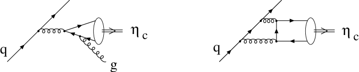
Figure 1: (a) A lowest-order diagram contributing to the process $q\to\eta_{c}+X$. (b) A higher-order diagram with no gluon emission. In each case there is another diagram with the $c$-quark–gluon vertices interchanged.

At lowest order, $q\rightarrow\eta_{c}+X$ fragmentation is due to the process $q\rightarrow q\eta_{c}g$ of Fig. 1a. The emission of the gluon suggests that this process may have a softer fragmentation function than the higher-order process $q\rightarrow q\eta_{c}$ shown in Fig. 1b. Due to the trigger bias effect, the higher-order process could be enhanced.

2. Results

Our calculation of the $q\to\eta_{c}+X$ fragmentation processes shown in Fig. 1 is described in the Appendix. The contribution of the lowest-order process (Fig. 1a) to the fragmentation function is of the form

$$D^{(a)}_{{\!\!}_{q\to\eta_{c}}}(z,\mu)=f(z)\ln\left({\mu^{2}\over 4m_{c}^{2}}\right)+g(z)+{\cal O}\left({4m_{c}^{2}\over\mu^{2}}\right).$$ (4)

The coefficient functions are

$$f(z) = {\alpha_{s}^{3}C_{F}\left|R_{S}(0)\right|^{2}\over 48\pi^{2}m_{c}^{3}N_{c}}\Biggl{\{}6\,\left(2+z\right)\left[{{\pi}^{2}\over 6}-{\cal L}_{2}(z)\right]-3\,z\,\ln(z)$$ (5)

$$\mbox{}+{2\over z}-18+12\,z+4\,{z^{2}}+\left(6+{6\over z}-12\,z\right)\,\ln(1-z)\Biggr{\}},$$

$$g(z) = {\alpha_{s}^{3}C_{F}\left|R_{S}(0)\right|^{2}\over 48\pi^{2}m_{c}^{3}N_{c}}\Biggl{\{}{{\pi}^{2}}\,\left(2+z\right)\,\ln(z)+\left(-18+{2\over z}+18\,z+4\,{z^{2}}\right)\,\ln(z)$$ (6)

$$\mbox{}+\left(6+{6\over z}-12\,z\right)\,\ln(1-z)\,\ln(z)-3\,z\,{{\ln(z)}^{2}}+34+{{\pi}^{2}}\,\left({1\over z}-2\right)$$

$$\mbox{}-{{71}\over{6\,z}}-{{53\,z}\over 2}+{{13\,{z^{2}}}\over 3}+\left({{-5}\over z}+9\,z-4\,{z^{2}}\right)\,\ln(1-z)$$

$$\mbox{}+\left(18-12\,z\right)\,{\cal L}_{2}(z)+6\,\left(2+z\right)\,\left[{\cal L}_{3}(z)-\ln(z)\,{\cal L}_{2}(z)-\zeta(3)\right]\Biggr{\}},$$

where

$${\cal L}_{2}(z)=-\int_{0}^{z}\frac{\ln(1-t)}{t}\;dt$$ (7)

is the dilogarithmic function,

$${\cal L}_{3}(z)=\int_{0}^{z}\frac{{\cal L}_{2}(t)}{t}\;dt,$$ (8)

and $\zeta(3)\approx 1.202$. The logarithmic term $f(z)\ln[\mu^{2}/(4m_{c}^{2})]$ arises from the two-step process where $q\to qg$ splitting is followed by $g\to\eta_{c}g$ fragmentation; the function $f(z)$ can be written as

$$f(z)=\int_{z}^{1}{dy\over y}P_{{\!}_{q\to g}}(z/y)D_{{\!\!}_{g\to\eta_{c}}}(y),$$ (9)

where $P_{{\!}_{q\to g}}(z/y)$ is the standard $q\to qg$ splitting function [14] and $D_{{\!\!}_{g\to\eta_{c}}}(y)$ is the $g\to\eta_{c}g$ fragmentation function at lowest order [1]. A similar result has been obtained in the case of $J/\psi$ production by light quark fragmentation [12, 13].

A lower limit of the loop contribution (see Fig. 1b) is obtained by considering only the imaginary part of the loop amplitude. There is no logarithmic term in this case:

$$D^{(b)}_{{\!\!}_{q\to\eta_{c}}}(z,\mu)\geq h(z)+{\cal O}\Bigl{(}{4m_{c}^{2}\over\mu^{2}}\Bigr{)},$$ (10)

where

$$h(z) = {\alpha_{s}^{4}\left|R_{S}(0)\right|^{2}C_{F}^{2}\over 96\pi m_{c}^{3}N_{c}}\Biggl{\{}14(1-z)\left[{\pi^{2}\over 6}-{\cal L}_{2}(1-z)\right]$$ (11)

$$\mbox{}+z+{2z\over 1-z}\ln(z)+{z(7z^{2}-18z+12)\over(1-z)^{2}}\ln^{2}(z)\Biggr{\}}.$$

The functions $f(z)$, $-g(z)$ and $h(z)$ are plotted in Fig. 2, using $\alpha_{s}=0.26$, $|R_{S}(0)|^{2}=(0.8\;{\rm GeV})^{3}$, and $m_{c}=1.5\;{\rm GeV}$. The loop contribution dominates over the lower-order Born contribution for $z\buildrel>\over{{}_{\sim}}0.3$, even though the real part of the loop was neglected. More quantitatively, the fifth moments of the Born and loop contributions have the numerical values

$${D}^{(5,a)}_{q\to\eta_{c}}(\mu)=\int_{0}^{1}dzz^{4}D_{q\to\eta_{c}}(z,\mu)\approx\left[2.4\ln\left({\mu^{2}\over 4m_{c}^{2}}\right)-5.1\right]\times 10^{-7},$$ (12)

$${D}^{(5,b)}_{q\to\eta_{c}}(\mu)\geq\int_{0}^{1}dzz^{4}h(z)\approx 1.1\times 10^{-6}.$$ (13)

Depending on the fragmentation scale $\mu$, the contribution from the loop diagram is thus up to an order of magnitude larger than the lowest-order Born contribution. Neglecting the higher-order process would lead to a major underestimate of the fragmentation cross section.

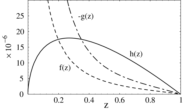
Figure 2: The functions $f(z)$, $-g(z)$ and $h(z)$ as defined in the text.

It is possible to further simplify the calculation of the fragmentation functions by taking advantage of the fact that only the large $z$ region is important, due to the trigger bias effect. We have verified that using only the leading part of an expansion of $D(z,\mu)$ around $z=1$ changes the fifth moments of the loop and Born contributions by less than 10%.

3. Discussion

The trigger bias effect in large $p_{T}$ quarkonium production favors fragmentation processes where the quarkonium takes a large fraction $z$ of the momentum of the fragmenting parton. When estimating the relative importance of different fragmentation processes, the shape of their $z$ dependence must therefore be considered.

In particular, some higher-order perturbative contributions may be enhanced relative to the lowest-order contributions due to the trigger bias effect. In this paper, we analyzed the process $q\to\eta_{c}+X$, where such an enhancement can be expected because gluon emission is not required in higher-order processes. We found that there is a loop contribution which indeed dominates the Born contribution by a large factor.

It is likely that an analogous result is obtained in the case of $q\to J/\psi$ fragmentation. Some relevant Born and loop diagrams are shown in Fig. 3. At higher orders, all the gluons coupling to the heavy quark line can be attached to the light quark line instead of being emitted, which suggests a hard $z$ dependence of the fragmentation function.

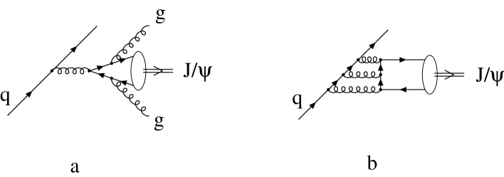
Figure 3: Light quark fragmentation into a $J/\psi$.

These higher-order contributions are part of the standard perturbation series and thus do not bring in any new parameters. Their relative importance should depend only weakly on the quark mass (through the decrease of $\alpha_{s}(m_{Q})$ with $m_{Q}$). This is in qualitative agreement with total cross section data [2, 3, 5, 6], which shows a disagreement with Born term calculations (within the colour singlet model) of similar magnitude for bottomonium and for charmonium.

The calculation presented here is not, however, immediately applicable to the present data on quarkonium production. The primary production mechanism for quarkonia at large $p_{T}$ in hadron collisions is expected to be gluon fragmentation. Even at higher orders, a minimum of two extra gluons need to accompany a produced $J/\psi$, due to charge conjugation invariance (cf. Fig. 4). In this case, loop diagrams like the one in Fig. 4b simply represent radiative corrections to the lowest-order process. Whether they enhance the kinematic region where the emitted gluons carry little momentum (the large $z$ region) can only be determined by an explicit calculation.

On the other hand, processes such as the one in Fig. 3b could be significant in collisions where light quarks are more copiously produced relative to gluons, such as at HERA. There, however, also charm quark fragmentation becomes important as a charmonium production mechanism at large $p_{T}$ [15].

In summary, we have pointed out that the trigger bias enhancement of large $z$ fragmentation is crucial in quarkonium production at large $p_{T}$. As a specific example, we considered the $q\to\eta_{c}$ fragmentation process and calculated a higher-order perturbative correction whose contribution to the cross section exceeds the lowest-order fragmentation contribution by a large factor.

Acknowledgement. We are grateful for discussions with Stan Brodsky.

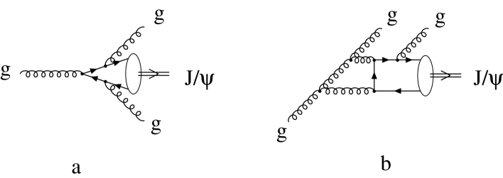
Figure 4: Gluon fragmentation into a $J/\psi$. (a) A lowest-order diagram. (b) A higher order diagram.

Appendix

We describe here our calculation of the $q\to\eta_{c}$ fragmentation functions. As shown in Figs. 5 and 6a, we denote by $p$ the momentum of the quarkonium state; $Q$ denotes the momentum of the fragmenting light quark, and $s=Q^{2}$ is its virtuality.

We work in the center of mass system of the light quark production process, and choose the third axis along the direction of the fragmenting light quark. The light-cone components of a four-vector $v$ are defined as $v^{\pm}=v^{0}\pm v^{3}$ and $\vec{v}_{\bot}=(v^{1},v^{2})$. The variable $z$ is defined as $z=p^{+}/Q^{+}$, which in the limit of large $Q^{+}$ is the fraction of the light quark momentum taken by the $\eta_{c}$.

We use an axial gauge with the polarization tensor

$${\cal P}^{\mu\nu}(k,n)=g^{\mu\nu}-{k^{\mu}n^{\nu}+n^{\mu}k^{\nu}\over n\cdot k},$$ (14)

where the gauge vector $n$ satisfies $n^{2}=0$, and $n\,\cdot\,v=v^{+}/Q^{+}$.

Let us write the matrix element for light quark production as $\bar{u}_{\alpha}(Q){\cal M}_{\alpha}$, where $\alpha$ is a Dirac index. The square of the amplitude for the full $\eta_{c}$ production process can then be written as ${\cal M}^{*}_{\beta}{\cal T}_{\beta\alpha}{\cal M}_{\alpha}$. In the limit of large $Q^{+}$,

$${\cal T}_{\beta\alpha}=T\parbox[b]{10.00002pt}{$Q$}\parbox[b]{8.00003pt}{ \raisebox{0.86108pt}{$/$} }_{\beta\alpha}+\dots$$ (15)

where $T$ is a scalar function. The full cross section then becomes a convolution of the light quark production rate

$$d\sigma=\left.\frac{1}{2E_{\rm CM}^{2}}\;{\rm dLips}\;{\cal M}^{*}_{\beta}\parbox[b]{10.00002pt}{$Q$}\parbox[b]{8.00003pt}{ \raisebox{0.86108pt}{$/$} }_{\beta\alpha}{\cal M}_{\alpha}\right|_{Q^{2}=0}$$ (16)

and a $q\to\eta_{c}$ fragmentation function which is given by a phase space integral of $T$, as shown below.

The leading-order fragmentation function

At lowest order, the $q\to\eta_{c}$ fragmentation function gets contributions only from the Feynman diagram of Fig. 5 and another diagram where the two $c$-quark–gluon vertices have been interchanged. The amplitudes corresponding to the two diagrams are equal.

As shown in Fig. 5, we denote the momentum of the virtual gluon by $k$ and define $w=k^{2}$ and $y=n\cdot k$.

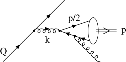
Figure 5: Momentum definitions in light quark fragmentation into $\eta_{c}$.

Let us first consider the square of the $q^{*}\to q\eta_{c}$ amplitude as it appears in the cross section of the full process. We find

$${\cal T} = \frac{128\pi^{2}\alpha_{s}^{3}C_{F}\left|R_{S}(0)\right|^{2}}{m_{c}N_{c}}\,{\parbox[b]{10.00002pt}{$Q$}\parbox[b]{8.00003pt}{ \raisebox{0.86108pt}{$/$} }\over s}\,\gamma^{\beta}\,(\parbox[b]{10.00002pt}{$Q$}\parbox[b]{8.00003pt}{ \raisebox{0.86108pt}{$/$} }-\parbox[b]{6.00006pt}{$k$}\parbox[b]{5.50003pt}{ \raisebox{-0.86108pt}{$/$} })\,\gamma^{\alpha}\,{\parbox[b]{10.00002pt}{$Q$}\parbox[b]{8.00003pt}{ \raisebox{0.86108pt}{$/$} }\over s}$$ (17)

$$\hskip 5.0pt\times{{\cal P}_{\alpha\alpha^{\prime}}(k,n)\over k^{2}}\;{p_{\rho}k_{\xi}\epsilon^{\rho\xi\alpha^{\prime}\mu}\over k^{2}-4m_{c}^{2}}\;\left[-{\cal P}_{\mu\nu}(k-p,n)\right]\;{p_{\rho^{\prime}}k_{\xi^{\prime}}\epsilon^{\rho^{\prime}\xi^{\prime}\beta^{\prime}\nu}\over k^{2}-4m_{c}^{2}}\;{{\cal P}_{\beta\beta^{\prime}}(k,n)\over k^{2}}$$

$$= T_{Q}\parbox[b]{10.00002pt}{$Q$}\parbox[b]{8.00003pt}{ \raisebox{0.86108pt}{$/$} }+T_{p}\parbox[b]{10.00002pt}{$p$}\parbox[b]{8.00003pt}{ \raisebox{0.86108pt}{$/$} }+T_{k}\parbox[b]{10.00002pt}{$k$}\parbox[b]{8.00003pt}{ \raisebox{0.86108pt}{$/$} }+T_{n}\parbox[b]{10.00002pt}{$n$}\parbox[b]{8.00003pt}{ \raisebox{0.86108pt}{$/$} }$$

$$= (T_{Q}+zT_{p}+yT_{k})\,\frac{1}{2}Q^{+}\gamma^{-}+\dots$$

$$= (T_{Q}+zT_{p}+yT_{k})\,\parbox[b]{10.00002pt}{$Q$}\parbox[b]{8.00003pt}{ \raisebox{0.86108pt}{$/$} }+\dots$$

The tensor $p_{\alpha}k_{\beta}\epsilon^{\alpha\beta\mu\nu}$ is due to the $c\bar{c}$ spin projection [16]. The dots in the last two expressions stand for terms of relative order $1/Q^{+}$. We made use of the fact that the coefficients $T_{Q},T_{p},T_{k},T_{n}$ depend only on scalar products of the four-momenta and are therefore independent of $Q^{+}$. Explicitly,

$$T = T_{Q}+zT_{p}+yT_{k}$$ (18)

$$= \frac{128\pi^{2}\alpha_{s}^{3}C_{F}\left|R_{S}(0)\right|^{2}}{m_{c}N_{c}}$$

$$\times{1\over 2s^{2}w^{2}(w-4m_{c}^{2})^{2}}\Biggl{[}-32\,{m_{c}^{4}}\,s-16\,{m_{c}^{4}}\,w-4\,\vec{p}_{\perp}^{\;2}\,s\,w-2\,s\,{w^{2}}-{w^{3}}$$

$$\mbox{}+{{2\,s\,\left(16\,{m_{c}^{4}}+2\,\vec{p}_{\perp}^{\;2}\,w+{w^{2}}\right)}\over y}+s\,\left(16\,{m_{c}^{4}}+{w^{2}}\right)\,y-{{2\,{{\left(4\,{m_{c}^{2}}+\vec{p}_{\perp}^{\;2}\right)}^{2}}\,w}\over{{z^{2}}}}$$

$$\mbox{}+{{2\,\left(4\,{m_{c}^{2}}+\vec{p}_{\perp}^{\;2}\right)\,w\,\left(4\,{m_{c}^{2}}+w\right)}\over z}-{{2\,s\,w\,\left(4\,{m_{c}^{2}}+w\right)\,z}\over y}-2\,{s^{2}}\,w\,{z^{2}}$$

$$\mbox{}-{{2\,{s^{2}}\,w\,{z^{2}}}\over{y^{2}}}+{{2\,s\,w\,\left(2\,s+w\right)\,{z^{2}}}\over y}\Biggr{]}.$$

The phase space measure for the full process can be written as the product of three factors: the phase space measure for light quark production, the phase space measure for the decay of the virtual light quark, and $ds/(2\pi)$. We write the two latter factors as

$$\int{ds\over(2\pi)}{d^{4}k\over(2\pi)^{4}}{d^{4}p\over(2\pi)^{4}}2\pi\delta^{+}((Q-k)^{2})2\pi\delta^{+}(p^{2}-4m_{c}^{2})2\pi\delta^{+}((k-p)^{2})\theta(\mu-s)$$

$$=\int_{\,0}^{\,1}dz\left[{1\over 256\pi^{4}}\int_{4m_{c}^{2}/z}^{\,\mu^{2}}\!\!\!\!ds\int_{\,z}^{\,1}{dy\over y}\int_{4m_{c}^{2}y/z}^{sy}\!\!\!\!dw\int_{-\sqrt{\rho}}^{\sqrt{\rho}}{dt\over\,\pi\sqrt{\rho-t^{2}}}\int{d\phi\over(2\pi)}\right]$$ (19)

where $\phi$ is the azimuthal angle of $\vec{p}_{\bot}$, and

$$\rho = {4z^{2}\over y^{4}}(1-y)(y-z)(s\,y-w)\left(w\,z-4m_{c}^{2}y\right),$$ (20)

$$t = \vec{p}_{\perp}^{\;2}+\left[{w\,z\over y^{2}}(2z-y-y\,z)+{z\over y}(s\,z-4m_{c}^{2})+4m_{c}^{2}+s\,z^{2}\right].$$ (21)

The integral over $z$ gives the convolution in the production cross section, and the leading-order light quark fragmentation function is

$$D_{{\!\!}_{q\to\eta_{c}}}(z,\mu) = \frac{1}{256\pi^{4}}\int_{4m_{c}^{2}/z}^{\,\mu^{2}}\!\!\!\!ds\int_{\,z}^{\,1}{dy\over y}\int_{4m_{c}^{2}y/z}^{sy}\!\!\!\!dw\int_{-\sqrt{\rho}}^{\sqrt{\rho}}{T\,dt\over\,\pi\sqrt{\rho-t^{2}}}$$ (22)

$$= f(z)\ln\left({\mu^{2}\over 4m_{c}^{2}}\right)+g(z)+{\cal O}\left({4m_{c}^{2}\over\mu^{2}}\right)+{\cal O}\!\left(\alpha_{s}^{4}\right).$$

Analytical expressions for the functions $f(z)$ and $g(z)$ are given in eqs. (5) and (6), respectively.

The loop contribution

The trigger bias enhanced NLO contribution to the $q\to\eta_{c}$ fragmentation function comes from the Feynman diagram in Fig. 6a, and another diagram where the two c-quark—gluon vertices have been interchanged. The amplitudes corresponding to these two diagrams are equal.

The four-momenta are defined in Fig. 6a. The loop momentum is denoted by $k$, and $y=n\cdot k$.

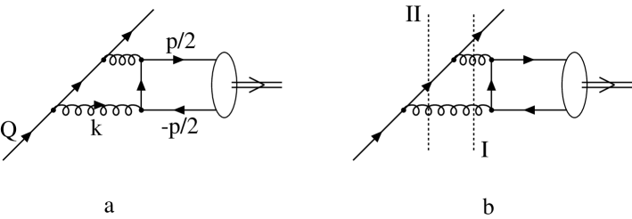
Figure 6: (a) Momentum definitions for the loop diagram contribution to $\eta_{c}$ production. (b) The cuts which give the imaginary part of the loop diagram.

We first consider the structure of the box loop integral

$$\Gamma=\int{d^{4}k\over(2\pi)^{4}}\;{\gamma^{\beta}(\parbox[b]{10.00002pt}{$Q$}\parbox[b]{8.00003pt}{ \raisebox{0.86108pt}{$/$} }-\parbox[b]{6.00006pt}{$k$}\parbox[b]{5.50003pt}{ \raisebox{-0.86108pt}{$/$} })\gamma^{\alpha}\over(Q-k)^{2}}\times{{\cal P}_{\alpha\mu}(k,n)\over k^{2}}\times{{\cal P}_{\beta\nu}(p-k,n)\over(p-k)^{2}}\times{p_{\alpha}k_{\beta}\epsilon^{\alpha\beta\mu\nu}\over(k^{2}-p\cdot k)}.$$ (23)

The four factors in the integrand of eq. (23) are easily identified with the four sides of the box loop of Fig. 6. Making a Dirac decomposition of the integrand we find

$$\Gamma=\parbox[b]{10.00002pt}{$A$}\parbox[b]{8.00003pt}{ \raisebox{0.86108pt}{$/$} }+i\parbox[b]{10.00002pt}{$B$}\parbox[b]{8.00003pt}{ \raisebox{0.86108pt}{$/$} }\gamma^{5}=\int{d^{4}k\over(2\pi)^{4}}(\parbox[b]{6.00006pt}{$a$}\parbox[b]{5.50003pt}{ \raisebox{-0.86108pt}{$/$} }+i\parbox[b]{6.00006pt}{$b$}\parbox[b]{5.50003pt}{ \raisebox{-0.86108pt}{$/$} }\gamma^{5}),$$ (24)

where

$$den\times a^{\mu} = \left[-y\,(k\!\cdot\!p)-z\,(k\!\cdot\!Q)+2m_{c}^{2}\,y+{s\,y\over 2}+k^{2}z\right]k_{\alpha}n_{\beta}p_{\gamma}\epsilon^{\alpha\beta\gamma\mu}$$ (25)

$$\mbox{}-z\,(k\!\cdot\!e)\,k^{\mu}+y\,(k\!\cdot\!e)\,p^{\mu},$$

$$den\times b^{\mu} = (1\!-\!y)\left[4m_{c}^{2}y+(z-2y)(k\!\cdot\!p)\right]k^{\mu}$$ (26)

$$\mbox{}-(1\!-\!y)\left[y(k\!\cdot\!p)-k^{2}(2y\!-\!z)\right]p^{\mu}$$

$$\mbox{}+\Biggl{[}(4m_{c}^{2}+s){y\over 2}(k\!\cdot\!p)-y(k\!\cdot\!p)^{2}-4m_{c}^{2}y(k\!\cdot\!Q)$$

$$\mbox{}+(2y\!-\!z)(k\!\cdot\!p)(k\!\cdot\!Q)+k^{2}\left({s\,z\over 2}+2m_{c}^{2}\,z-s\,y\right)\Biggr{]}\,n^{\mu},$$

and the denominators from the propagators and the gluon polarization tensors are included in

$$den=y(z-y)(Q-k)^{2}k^{2}(p-k)^{2}\left[k^{2}-(p\!\cdot\!k)\right].$$ (27)

Any four-vector $X^{\mu}$ can be written as a linear combination $X^{\mu}=X_{n}n^{\mu}+X_{Q}Q^{\mu}+X_{p}p^{\mu}+X_{e}e^{\mu}$ of $n$, $Q$, $p$ and $e^{\mu}=n_{\alpha}Q_{\beta}p_{\gamma}\epsilon^{\alpha\beta\gamma\mu}$. It is easily seen that $a_{p}(k)$, $a_{Q}(k)$, $a_{n}(k)$, and $b_{e}(k)$ are all antisymmetric when $k$ is mirrored in the hyper plane spanned by $n,p$ and $Q$, i.e. when $k_{e}\to-k_{e}$. Therefore they do not contribute to the integral, and

$$A^{\mu} = A_{e}e^{\mu}=\int{d^{4}k\over(2\pi)^{4}}a_{e}(k)e^{\mu},$$ (28)

$$B^{\mu} = B_{n}n^{\mu}+B_{Q}Q^{\mu}+B_{p}p^{\mu}$$ (29)

$$= \int{d^{4}k\over(2\pi)^{4}}\left[b_{n}(k)n^{\mu}+b_{Q}(k)Q^{\mu}+b_{p}(k)p^{\mu}\right].$$

Analogously with eq. (17), we now find

$${\cal T} = \frac{\pi\alpha_{s}^{4}\left|R_{S}(0)\right|^{2}C_{F}^{2}}{8N_{c}m_{c}^{5}}\;{\parbox[b]{10.00002pt}{$Q$}\parbox[b]{8.00003pt}{ \raisebox{0.86108pt}{$/$} }\over s}(\parbox[b]{10.00002pt}{$A$}\parbox[b]{8.00003pt}{ \raisebox{0.86108pt}{$/$} }^{*}-i\parbox[b]{10.00002pt}{$B$}\parbox[b]{8.00003pt}{ \raisebox{0.86108pt}{$/$} }^{*}\gamma^{5})(\parbox[b]{10.00002pt}{$Q$}\parbox[b]{8.00003pt}{ \raisebox{0.86108pt}{$/$} }-\parbox[b]{6.00006pt}{$p$}\parbox[b]{5.50003pt}{ \raisebox{-0.86108pt}{$/$} })(\parbox[b]{10.00002pt}{$A$}\parbox[b]{8.00003pt}{ \raisebox{0.86108pt}{$/$} }+i\parbox[b]{10.00002pt}{$B$}\parbox[b]{8.00003pt}{ \raisebox{0.86108pt}{$/$} }\gamma^{5}){\parbox[b]{10.00002pt}{$Q$}\parbox[b]{8.00003pt}{ \raisebox{0.86108pt}{$/$} }\over s}$$ (30)

$$= K_{Q}\parbox[b]{10.00002pt}{$Q$}\parbox[b]{8.00003pt}{ \raisebox{0.86108pt}{$/$} }+K_{p}\parbox[b]{6.00006pt}{$p$}\parbox[b]{5.50003pt}{ \raisebox{-0.86108pt}{$/$} }+K_{n}\parbox[b]{6.00006pt}{$n$}\parbox[b]{5.50003pt}{ \raisebox{-0.86108pt}{$/$} }+iK_{\parbox[b]{4.20004pt}{$e$}\parbox[b]{3.85002pt}{ \raisebox{-0.60275pt}{$/$} }\gamma^{5}}\parbox[b]{6.00006pt}{$e$}\parbox[b]{5.50003pt}{ \raisebox{-0.86108pt}{$/$} }\!\gamma^{5}$$

$$= (K_{Q}+zK_{p})\parbox[b]{10.00002pt}{$Q$}\parbox[b]{8.00003pt}{ \raisebox{0.86108pt}{$/$} }+\dots$$

$$= \frac{\pi\alpha_{s}^{4}\left|R_{S}(0)\right|^{2}C_{F}^{2}}{8N_{c}m_{c}^{5}}\;{1-z\over s^{2}}|C|^{2}\parbox[b]{10.00002pt}{$Q$}\parbox[b]{8.00003pt}{ \raisebox{0.86108pt}{$/$} }+\dots,$$

where

$$C = (s\,z-4m_{c}^{2})A_{e}-(2B_{n}+s\,B_{Q}+s\,B_{p})$$ (31)

$$= \int{d^{4}k\over(2\pi)^{4}}\Bigl{[}(s\,z-4m_{c}^{2})a_{e}-(2b_{n}+s\,b_{Q}+s\,b_{p})\Bigr{]}.$$

The phase space measure for the decay of the virtual light quark times $ds/(2\pi)$ is in this case

$$\frac{1}{32\pi^{3}}\int_{0}^{1}dz\int_{4m_{c}^{2}/z}^{\mu^{2}}ds\int_{0}^{2\pi}d\phi.$$ (32)

As $C$ is independent of the azimuthal angle $\phi$ of the decay, we obtain the following ’box’ contribution to the light quark fragmentation function:

$$D_{q\to\eta_{c}}^{\rm(box)}(z,\mu)=\frac{\alpha_{s}^{4}\left|R_{S}(0)\right|^{2}C_{F}^{2}}{128\pi N_{c}m_{c}^{5}}\int_{4m_{c}^{2}/z}^{\mu^{2}}ds{(1-z)\over s^{2}}|C|^{2}.$$ (33)

We have only calculated the imaginary part of the box amplitude, which is due to the sum of the two Cutkosky cuts $I$ and $I\!I$ of Fig. 6b. This gives a lower limit of the full loop contribution. The imaginary part is obtained by replacing, respectively,

$$\int{d^{4}k\over(2\pi)^{4}} \stackrel{{\scriptstyle I}}{{\to}} {1\over 2}\int{d^{4}k\over(2\pi)^{4}}\,k^{2}\,(p-k)^{2}\,2\pi\delta^{+}(k^{2})\,2\pi\delta^{+}((p-k)^{2})$$

$$\int{d^{4}k\over(2\pi)^{4}} \stackrel{{\scriptstyle I\!I}}{{\to}} {1\over 2}\int{d^{4}k\over(2\pi)^{4}}\,k^{2}\,(Q-k)^{2}\,2\pi\delta^{+}(k^{2})\,2\pi\delta^{+}((Q-k)^{2})$$ (34)

in eq. (31). We find

$${\rm Im}(C) = C^{I}+C^{I\!I}={4m_{c}^{2}s\over s-4m_{c}^{2}}\left[1-{2s-4m_{c}^{2}\over s-4m_{c}^{2}}\ln\left(s\over 4m_{c}^{2}\right)\right],$$ (35)

$$C^{I} = {s\,z\over 1-z}\ln\left((s-4m_{c}^{2})z\over s\,z-4m_{c}^{2}\right).$$ (36)

Performing the $s$ integration we get the result given in eqs. (10,11).

References

[1]
E. Braaten and T. C. Yuan,
Phys. Rev. Lett. 71, 1673 (1993).
[2]
CDF Collaboration, F. Abe et al.,
Phys. Rev. Lett. 75, 4358 (1995); Phys. Rev. Lett. 69, 3704 (1992); CDF Collaboration, V. Papadimitriou et al.,
Report No. Fermilab-Conf-95/128-E, presented at 30th Rencontres de
Moriond: QCD and High Energy Hadronic Interactions,
Meribel les Allues, France, March 1995.
[3]
D0 Collaboration, S. Abachi et al.,
Reports No. Fermilab-Conf-95/205-E and Fermilab-Conf-95/206-E,
submitted to International Europhysics Conference on High Energy Physics
(HEP 95), Brussels, Belgium, July-August 1995.
[4] R. Baier and R. Rückl, Z. Phys. C19, 251 (1983),
and references therein.
[5] G. A. Schuler, Report No. CERN-TH.7170/94, hep-ph/9403387, to appear in Phys. Rep.
[6]
M. Vänttinen, P. Hoyer, S. J. Brodsky and Wai-Keung Tang,
Phys. Rev. D 51, 3332 (1995).
[7]
E. Braaten, M. A. Doncheski, S. Fleming and M. Mangano,
Phys. Lett. B333, 548;
M. Cacciari and M. Greco, Phys. Rev. Lett. 73, 1586 (1994);
D. P. Roy and K. Sridhar, Phys. Lett. B339, 141 (1994).
[8] E. Braaten and S. Fleming,
Phys. Rev. Lett. 74, 3327 (1995).
[9] G. T. Bodwin, E. Braaten and G. P. Lepage,
Phys. Rev. D 51, 1125 (1995).
[10] P. Cho and M. B. Wise,
Phys. Lett. B346, 129 (1995).
[11] Wai-Keung Tang and M. Vänttinen,
Report No. SLAC-PUB-95-6931, hep-ph/9506378,
to appear in Phys. Rev. D.
[12] K. Cheung, W.-Y. Keung and T. C. Yuan,
Report No. Fermilab-Pub-95-300-T (1995), hep-ph/9509308.
[13] P. Cho, Report No. CALT-68-2020 (1995), hep-ph/9509355.
[14] G. Altarelli and G. Parisi,
Nucl. Phys. B126, 298 (1977).
[15] R. M. Godbole, D. P. Roy and K. Sridhar,
Report No. TIFR-TH-95-57, hep-ph/9511433.
[16] J. H. Kühn, J. Kaplan and E. G. O. Safiani,
Nucl. Phys. B157, 125 (1979).