CERN-TH/96-20

UGVA–DPT 1996/01–912

hep-ph/9601324

$R_{b}$, $R_{c}$ and Jet Distributions
at the Tevatron in a Model
with an Extra Vector Boson
Guido ALTARELLI${}^{\,a,b}$, Nicola DI BARTOLOMEO${}^{\,c}$,

Ferruccio FERUGLIO${}^{\,d}$, Raoul GATTO${}^{\,c}$ and

Michelangelo L. MANGANO${}^{\,a}$ ^a CERN, Theory Division,
1211 Geneva 23, Switzerland
^b Dipartimento di Fisica, Universita’ di Roma III, Italy
^c Département de Physique Théorique, Université de
Genève, CH-1211 Geneva 4, Switzerland
^d Dipartimento di Fisica, Universita’ di Padova, and
INFN, Sezione di Padova, Italy

We show that the reported anomalies in $R_{b}$ and $R_{c}$ can be interpreted as the effect of a heavy vector boson $V$ universally coupled to $u$- and $d$-type quarks separately and nearly decoupled from leptons. This extra vector boson could then also naturally explain the apparent excess of the jet rate at large transverse momentum observed at CDF.

CERN-TH/96-20
January 1996

1 Introduction

On the whole the electroweak (EW) precision tests performed at LEP, SLC and at the Tevatron have impressively confirmed the formidable accuracy of the Standard Model (SM) predictions. There are only a few hints of possible deviations and our hopes of finding new physics signals are confined to them. At LEP the observed values of $R_{b}$ and $R_{c}$ deviate from the SM predictions by about 3.5$\sigma$ and 2.5$\sigma$, respectively [1]. At CDF an excess of jets at large $E_{\rm T}$ with respect to the QCD prediction has been reported [2]. None of these observations provides a very compelling evidence for new physics as yet, because of the limited statistics and of possible residual experimental systematics. The $R_{b}$ value is relatively more established, in the sense that it was first announced in 1993 and is insofar supported by the analyses of all four LEP collaborations with several independent, in principle clean, tagging methods. From a speculative point of view it is not implausible to have a deviation in the third generation sector. Also, a moderate increase of $R_{b}$ with respect to the SM (of roughly half of the present excess) would bring the value of $\alpha_{s}(M_{Z})$ measured from the $Z$ widths in even better agreement with lower energy determinations. The $R_{c}$ evidence is much less believable both from the experimental and the theoretical points of view. In absolute terms it is a large deficit, that would overcompensate the $R_{b}$ excess. Thus these results, if taken at face value, would demand a deviation from the SM in the light-quark widths as well, in order to reestablish the observed value of $\Gamma_{h}$, which is measured with great experimental accuracy and agrees with the SM. After all, in this context charm is alike any other first or second generation quark, while beauty could be special, being connected to the heavy top. If one literally believes the data, then one must accept an accurate cancellation among the new physics contributions to light and heavy quarks. But the perfect agreement of the leptonic widths with the SM, up to a fraction of MeV, clearly poses the problem of how to naturally shift the light quark widths without affecting the leptonic ones as well. Finally, the significance of the CDF result on jets entirely depends on the calculation of the QCD predictions at large $E_{\rm T}$, which could to some extent be questioned. For example, it was recently pointed out [3] that it is possible to slightly increase the large-$x$ gluon densities without deteriorating the standard overall fits to low energy data, and thus partly explain a large fraction of the high-$E_{\rm T}$ jet discrepancy.

All these words of caution being said, in this note we consider the challenging task of quantitatively explaining in an admittedly ad hoc but relatively simple model all the three observed deviations discussed above. We introduce a heavy vector neutral resonance $V$, singlet with respect to the standard gauge group $SU(3)\times SU(2)_{L}\times U(1)_{Y}$ and with a mass in the TeV range. We allow this new resonance $V$ to have a small mixing with the ordinary $Z$ gauge boson, and therefore to contribute to the $Z$ decays. We observe that while in the data $\delta(R_{b}+R_{c})$ is large and negative, $\delta(3R_{b}+2R_{c})$ is only about $1\sigma$ away from zero. This suggests to take universal couplings of the $V$ to the three generations of fermions separately for up, down and charged leptons. Since the leptonic width is in perfect agreement with the SM, the leptonic couplings of $V$ must be much smaller than those needed for the quarks to explain the deviations observed via $\delta R_{b}$ and via $\delta R_{c}$, and we shall take them as approximately vanishing (at a less phenomenological level, one must be prepared to add new, presumably very heavy, fermions to compensate the anomalies). Then the products of the amount of mixing (which is severely constrained by the data) times the couplings of the $V$ to up- and down-type quarks are fixed by imposing that the observed values of $\delta R_{b}$ and of $\delta(3R_{b}+2R_{c})$ be approximately reproduced. We have at our disposal five parameters to do that: the amount of mixing, $M_{V}$ (that for a given mixing fixes $\epsilon_{1}=\delta\rho$), the left-handed coupling to the $(u,d)_{\rm L}$ doublets, and the two right-handed couplings to the $u_{\rm R}$ and $d_{\rm R}$ singlets. So the game would be trivial, were it not for the fact that couplings to quarks as large as those required by $\delta R_{b}$ and $\delta R_{c}$ would tend to produce too large effects in the distributions of large-$E_{\rm T}$ jets measured at the Tevatron. We can then adjust $\mbox{$M_{V}$}\geq 1$ TeV and the left and right couplings in such a way as to obtain a reasonable fit to both LEP and CDF anomalies, without violating, to our knowledge, any known experimental constraint. The details are given in what follows.

2 Effects on LEP and SLC observables

The tree level neutral current interaction can be written in terms of the unmixed interaction states $Z_{0}$ and $V_{0}$, coupled respectively to the ordinary standard model neutral current $(J_{3L}-\sin^{2}\theta_{W}J_{em})$ and to an additional current $J_{N}$. The vector and axial couplings of the gauge bosons $Z_{0}$ and $V_{0}$ are defined by:

$${\cal L}_{NC} = {g\over 2\cos\theta_{W}}\sum_{i}\left[Z_{0}^{\mu}(v_{S}^{i}{\bar{\psi}}^{i}\gamma_{\mu}\psi^{i}+a_{S}^{i}{\bar{\psi}}^{i}\gamma_{\mu}\gamma_{5}\psi^{i})\right.$$ (2.1)

$$+ \left.V_{0}^{\mu}(v_{N}^{i}{\bar{\psi}}^{i}\gamma_{\mu}\psi^{i}+a_{N}^{i}{\bar{\psi}}^{i}\gamma_{\mu}\gamma_{5}\psi^{i})\right]$$

The $Z_{0}$ couplings are the standard ones

$$v_{S}^{i}=T^{i}_{3L}-2\sin^{2}\theta_{W}Q^{i}\;,~{}~{}~{}a_{S}^{i}=-T^{i}_{3L}$$ (2.2)

where $T^{i}_{3L}$ is the third component of the weak isospin of the fermion $i$, and $Q^{i}$ its electric charge.

We assume that the new gauge boson $V_{0}$ couples only to the quarks and has zero (or negligible) couplings to the leptons. We also assume family-independent couplings. The new interactions can be then be expressed in terms of three parameters $x$, $y_{u}$ and $y_{d}$:

$$v_{N}^{u}=x+y_{u}~{}~{} ~{}~{}a_{N}^{u}=-x+y_{u}$$ ,

$$v_{N}^{d}=x+y_{d}~{}~{} ~{}~{}a_{N}^{d}=-x+y_{d},$$ , (2.3)

where the superscripts $u$ and $d$ refer to up-type and down-type quarks.

In presence of a mixing, the mass eigenstates $Z$ and $V$ are given by a rotation of the unmixed states $Z_{0}$ and $V_{0}$:

$$Z = \cos\xi Z_{0}+\sin\xi V_{0}$$

$$V = -\sin\xi Z_{0}+\cos\xi V_{0}$$ (2.4)

Due to the mixing, the $\rho$ parameter, defined by

$$\rho={M_{W}^{2}\over M_{Z}^{2}\cos^{2}\theta_{W}}$$ (2.5)

receives a tree level contribution $\Delta\rho_{M}$, which in term of the $V$ mass and the mixing angle $\xi$ is given by:

$$\Delta\rho_{M}=\left[\left({M_{V}\over M_{Z}}\right)^{2}-1\right]\sin^{2}\xi\simeq\left({\mbox{$M_{V}$}\over M_{Z}}\right)^{2}\,\xi^{2}$$ (2.6)

At LEPI the observables get corrections from the presence of $V$ through the mixing with the ordinary $Z$ and through the shift in the $\rho$ parameter. Contributions from direct $V$ exchange are negligible at the $Z$ pole, but will be taken into account later on in our study of the Tevatron jet observables.

The deviation of a LEPI observable, linearized in $\Delta\rho_{M}$ and $\xi$, can therefore be expressed as:

$${\delta{\cal O}\over{\cal O}}=A_{\cal O}\Delta\rho_{M}+B_{\cal O}\xi.$$ (2.7)

The coefficients $A_{\cal O}$ are universal and depend only on the SM parameters and couplings, while $B_{\cal O}$ also depend on the $V_{0}$ couplings $v^{i}_{N}$ and $a^{i}_{N}$ [4]. In Table I we give the numerical values of $A_{\cal O}$ and the expressions for $B_{\cal O}$ for the observables of interest, as functions of the parameters $x$, $y_{u}$ and $y_{d}$ introduced in eq. (2.3). In Table I we also present the experimental data used in the present analysis [1], together with the Standard Model predictions [5] for $m_{top}=175$ GeV, $m_{H}=300$ GeV and $\alpha_{s}(M_{Z})=0.125$. They include the one-loop electroweak radiative corrections. The $Z$ mass was fixed at the experimental value $M_{Z}=91.1887$ GeV.

Quantity	$A$	$B$	Exp. values [1]	SM values	Pull of the fit
${\Gamma_{Z}}$	1.36	$-0.92x-0.49y_{u}+0.37y_{d}$	$2496.3\pm 3.2$	2497.4	1.72
$R_{l}=\Gamma_{h}/\Gamma_{l}$	0.34	$-1.31x-0.70y_{u}+0.52y_{d}$	$20.788\pm 0.032$	20.782	$-0.35$
$\sigma_{h}$	$-0.030$	$0.52x+0.28y_{u}-0.21y_{d}$	$41.488\pm 0.078$	41.451	$-0.32$
$R_{b}=\Gamma_{b}/\Gamma_{h}$	$-0.094$	$-3.16x+0.70y_{u}+0.29y_{d}$	$0.2219\pm 0.0017$	0.21569	$-1.41$
$R_{c}=\Gamma_{c}/\Gamma_{h}$	0.12	$6.20x-1.43y_{u}-0.59y_{d}$	$0.1543\pm 0.0074$	0.17238	1.62
$M_{W}/M_{Z}$	0.71	0	$0.8802\pm 0.0018$	0.8808	0.94
${\cal A}_{l}$	18.50	0	$-0.15066\pm 0.00276$	$-0.14334$	0.98
${\cal A}_{b}$	0.23	$-0.31x-1.72y_{d}$	$-0.841\pm 0.053$	$-0.9342$	$-1.79$
${\cal A}_{c}$	1.70	$2.37x+5.36y_{u}$	$-0.606\pm 0.090$	$-0.6662$	$-1.00$
$A_{FB}^{b}$	18.15	$-0.31x-1.72y_{d}$	$0.0999\pm 0.0031$	0.10042	1.20
$A_{FB}^{c}$	19.63	$2.37x+5.36y_{u}$	$0.0725\pm 0.0058$	0.07161	0.76

Table I : Coefficients $A$ and $B$, defined in eq. (2.7), for various electroweak observables, together with their experimental values and SM theoretical predictions for $m_{top}=175\;GeV$, $m_{H}=300\;GeV$ and $\alpha_{s}(M_{Z})=0.125$. The corresponding $\chi^{2}$ is equal to 26.73. In the last column we report the pull values ((fit-exp)/$\sigma$) for the final $V$ fit with $x=-1$, $y_{u}=2.2$, $y_{d}=0$ and $\xi=3.8\cdot 10^{-3}$. The $\chi^{2}$ in this case equals 14.72.

The deviations in Table I are computed from the tree level formulas for the partial widths

$$\Gamma(Z\rightarrow{\bar{f}}f)={G_{F}M_{Z}^{3}\over 6\pi\sqrt{2}}\rho N_{c}\left[(v_{eff}^{f})^{2}+(a_{eff}^{f})^{2}\right],$$ (2.8)

and for the asymmetries

$${\cal A}_{f}={2a_{eff}^{f}v_{eff}^{f}\over(v_{eff}^{f})^{2}+(a_{eff}^{f})^{2}}.$$ (2.9)

The forward-backward asymmetries are given by:

$$A_{FB}^{f}={3\over 4}{\cal A}_{e}{\cal A}_{f}$$ (2.10)

In eq. (2.8) $N_{c}=3$ for quarks and $N_{c}=1$ for leptons, and in eq. (2.8) and (2.9) the effective vector and axial-vector coupling $v_{eff}^{f}$ and $a_{eff}^{f}$ are superpositions of the corresponding $Z_{0}$ and $V_{0}$ couplings:

$$v_{eff}^{f}=\cos\xi\,v_{S}^{f}+\sin\xi\,v_{N}^{f}$$

$$a_{eff}^{f}=\cos\xi\,a_{S}^{f}+\sin\xi\,a_{N}^{f}$$ (2.11)

In computing the deviations due to the new vector resonance $V$, it is sufficient to consider the tree level expressions for the observables, because the corrections are proportional to $\Delta\rho_{M}$ or $\xi$, that are both constrained to be quite small (of the order $10^{-3}$) by the current electroweak data.

We keep fixed the input parameters $\alpha$, $G_{F}$, $M_{Z}$, and take into account the modification of the effective Weinberg angle given in eq. 2.5 because of the shift in the $\rho$ parameter. One finds [4]:

$$\delta(\sin^{2}\theta_{W})=-{\sin^{2}\theta_{W}\cos^{2}\theta_{W}\over\cos^{2}2\theta_{W}}\Delta\rho_{M}$$ (2.12)

The loop effects due to the heavy gauge boson $V$ are quite small and we will neglect them.

3 Fit to the LEP and SLC data

In this Section we constrain the free parameters of our extended gauge model by performing a fit of the eleven independent observables of Table I. The parameter space of the model includes the couplings $x$, $y_{u}$, $y_{d}$ and the two parameters $\xi$ and $M_{V}$. $\Delta\rho_{M}$ is related to the previous parameters by eq. (2.6).

We have minimized the $\chi^{2}$ function keeping $M_{V}$ fixed at different values: it turns out that the best fit central value for $\Delta\rho_{M}$ stays almost fixed, by varying $M_{V}$, at the value

$$\Delta\rho_{M}\simeq 0.0011$$ (3.13)

This implies, from eqs. (2.6), that the mixing angle $\xi$ decreases with $M_{V}$:

$$\xi\simeq\sqrt{0.0011}{M_{Z}\over M_{V}}$$ (3.14)

The parameters $x$, $y_{u}$, and $y_{d}$ are multiplied by the mixing angle $\xi$ in the expression (2.7) for the deviations: that means, from eq. (3.14), that their best fit values will scale with $M_{V}$ as $1/\xi$, i.e.

$$x,~{}y_{u},~{}y_{d}\sim{M_{V}\over M_{Z}}$$ (3.15)

The fit, for a choice $M_{V}=1000$ GeV, leaving the four parameters $\xi$, $x$, $y_{u}$, and $y_{d}$ as free, gives:

$$\xi=(3.0^{+0.9}_{-1.2})\cdot 10^{-3} ~{}x=-1.4^{+1.1}_{-1.9}$$ ,

$$y_{u}=5.3^{+4.1}_{-2.1} ~{}y_{d}=2.9^{+4.9}_{-4.6}$$ , (3.16)

We have quoted the standard errors, corresponding to $\chi^{2}=\chi^{2}_{min}+1$. The fit is weakly sensitive to the parameter $y_{d}$, as the large error indicates. We take advantage of this by constraining the fit with $y_{d}=0$. The other parameters of the fit with $y_{d}=0$ turn out to be:

$$\xi=(2.8^{+0.9}_{-1.4})\cdot 10^{-3}~{},~{}x=-2.1^{+0.8}_{-2.4}~{},~{}y_{u}=4.5^{+4.4}_{-1.5}$$ (3.17)

where we have fixed, as before, $M_{V}=1000$ GeV. Here $\chi^{2}=11.41$. For other values of $M_{V}$, the scaling formulas eq. (3.14) and (3.15) are an excellent approximation. The central values correspond to quite large couplings that would be incompatible with the CDF data, as shown in the next Section.

The parameters in eq. (3.17) are strongly correlated. The correlation between the parameters $x$ and $y_{u}$ is easily understood once noticed, from Table I, that the ratio of the coefficients multiplying $x$ and $y_{u}$ in the formulas for the deviations is the same, 1.87, in the observables $\Gamma_{Z}$, $R_{l}$ and $\sigma_{h}$. The relative high precision data are in excellent agreement with the SM predictions, and this induces a strong anticorrelation between the two parameters.

In fig. 1a we plot the $70\%$ confidence level ellipsis in the plane $y_{u}$ versus $x$, keeping $\xi$ fixed at the best-fit value $2.8\cdot 10^{-3}$. From the figure, one can see that at this confidence level the points closest to the origin are at the position $x\simeq-1.3$, $y_{u}\simeq 2.8$.

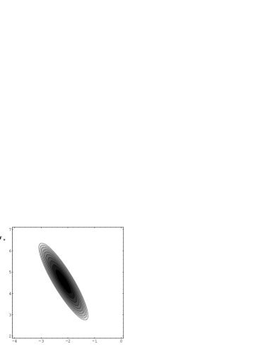
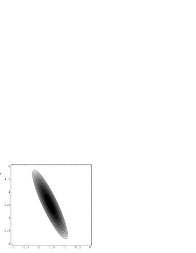
Figure 1: $70\%$ confidence level ellipsis in the plane $y_{u}$ versus $x$, for $M_{V}=1000$ GeV, $y_{d}=0$ and $\xi=2.8\cdot 10^{-3}$ (left figure) or $\xi=3.8\cdot 10^{-3}$ (right figure).

In fig. 1b we present the analogous ellipsis for the higher value $\xi=3.8\cdot 10^{-3}$. Increasing $\xi$, the elliptical region moves toward the origin, because the higher mixing angle forces the parameters $x$, $y_{u}$ to smaller values. For the value of $\xi=3.8\cdot 10^{-3}$ the closest points to the origin are located at $x\simeq-1.0$, $y_{u}\simeq 2.2$. Moving away from the best-fit value of $\xi$, the $\chi^{2}$ value increases: for $\xi=3.8\cdot 10^{-3}$, $x=-1.0$, and $y_{u}=2.2$, one obtains $\chi^{2}=\chi^{2}_{min}+3.3$, still in the $70\%$ confidence level region of the three parameters fit of eq. (3.17).

In the last column of Table I we quote the pull values, given by (fit - exp)/$\sigma$, for $\xi=3.8\cdot 10^{-3}$, $x=-1$, $y_{u}=2.2$ and $y_{d}=0$: the discrepancies in $R_{b}$ and $R_{c}$ are reduced. We stress again that these are not the best fit values for the parameters, but they lead to an effect on jet observables which is quite compatible with the CDF observations, as we shall now discuss.

4 Comparison with the Tevatron jet distributions

A vector resonance $V$ with such large couplings as obtained from the fits of the previous Section is liable to produce visible effects in hadronic collisions. There it can be directly produced via the Drell-Yan mechanism if the mass is not too large, or can lead to effective interactions between quarks via virtual exchange. The net result is a growth of the inclusive $E_{\rm T}$ distribution of jets at large $E_{\rm T}$, relative to the standard QCD expectations. Using the $V$couplings defined in eq. (2.3), it is easy to evaluate the following quark-quark scattering amplitudes (amplitudes for crossed channels can be easily obtained from these ones):

$${1\over(4\pi)^{2}} \overline{\sum}|A(qq\rightarrow qq)|^{2}\;=\;{1\over(4\pi)^{2}}\overline{\sum}|A_{QCD}(qq\rightarrow qq)|^{2}+$$ (4.18)

$${32\over 9}\mbox{$\alpha_{s}$}\mbox{$\alpha^{\prime}$}s^{2}{\cal{R}}\bigl{\{}{1\over t[(u-\mbox{$M_{V}^{2}$})+i\mbox{$M_{V}$}\mbox{$\Gamma_{V}$}]}+{1\over u[(t-\mbox{$M_{V}^{2}$})+i\mbox{$M_{V}$}\mbox{$\Gamma_{V}$}]}\bigr{\}}(x^{2}+y_{q}^{2})+$$

$$16\mbox{$\alpha^{\prime}$}^{2}\Bigl{\{}s^{2}(x^{4}+y_{q}^{4})\bigl{[}{1\over(t-\mbox{$M_{V}^{2}$})^{2}+\mbox{$M_{V}^{2}$}\mbox{$\Gamma_{V}$}^{2}}+{1\over(u-\mbox{$M_{V}^{2}$})^{2}+\mbox{$M_{V}^{2}$}\mbox{$\Gamma_{V}$}^{2}}+$$

$${2\over 3}{\cal{R}}{1\over(t-\mbox{$M_{V}^{2}$})+i\mbox{$M_{V}$}\mbox{$\Gamma_{V}$}}{1\over(u-\mbox{$M_{V}^{2}$})-i\mbox{$M_{V}$}\mbox{$\Gamma_{V}$}}\bigr{]}+$$

$$2x^{2}y_{q}^{2}\bigl{[}{u^{2}\over(t-\mbox{$M_{V}^{2}$})^{2}+\mbox{$M_{V}^{2}$}\mbox{$\Gamma_{V}$}^{2}}+{t^{2}\over(u-\mbox{$M_{V}^{2}$})^{2}+\mbox{$M_{V}^{2}$}\mbox{$\Gamma_{V}$}^{2}}\bigr{]}\Bigr{\}}$$

$${1\over(4\pi)^{2}} \overline{\sum}|A(qq^{\prime}\rightarrow qq^{\prime})|^{2}\;=\;{1\over(4\pi)^{2}}\overline{\sum}|A_{QCD}(qq^{\prime}\rightarrow qq^{\prime})|^{2}+$$ (4.19)

$${16\mbox{$\alpha^{\prime}$}^{2}\over(t-\mbox{$M_{V}^{2}$})^{2}+\mbox{$M_{V}^{2}$}\mbox{$\Gamma_{V}$}^{2}}\bigl{[}s^{2}\,(x^{4}+y_{q}^{2}y_{q^{\prime}}^{2})+u^{2}x^{2}\,(y_{q}^{2}+y_{q^{\prime}}^{2})\bigr{]}$$

where $A_{QCD}$ is the standard QCD amplitude, ${\cal R}$ denotes the real part, $\mbox{$\alpha^{\prime}$}=g^{2}/(16\pi\cos^{2}\theta_{W})\sim 0.010$ and $\Gamma_{V}$ is the $V$ total decay width given by:

$$\mbox{$\Gamma_{V}$}=2N_{g}\mbox{$\alpha^{\prime}$}\mbox{$M_{V}$}(2x^{2}+y_{u}^{2}+y_{d}^{2})$$ (4.20)

Taking the $\mbox{$M_{V}$}\rightarrow\infty$ limit one recovers the standard results obtained in presence of an effective 4-quark coupling [6] .

Figure 2: The effect of $V$ exchange on the inclusive $E_{\rm T}$ distribution of jets at the Tevatron. The different curves correspond to increasing values of $y_{u}$, from 2 to 4. The four displays correspond to $x=-0.5$, –1, –1.5 and –2. The quantity $(CDF-QCD)/QCD$ [2] is shown by the points. We used dashed or continuous lines to indicate whether the $V$ width is smaller or larger than 500 GeV.

Figure 3: The effect of $V$ exchange on the invariant mass distribution of di-jet events at the Tevatron. The different curves correspond to increasing values of $y_{u}$ from 2 to 4. The four displays correspond to $x=-0.5$, –1, –1.5 and –2. The quantity $(CDF-QCD)/QCD$ [7] is shown by the points.

Fig. 2 shows the deviations induced by the couplings to the $V$ on the jet inclusive $E_{\rm T}$ distribution at the Tevatron. The quantity:

$$\bigl{[}{d\sigma^{(QCD+V)}/d\mbox{$E_{\rm T}$}\over d\sigma^{QCD}/d\mbox{$E_{\rm T}$}}\bigr{]}_{\eta=0}-1$$ (4.21)

is plotted as a function of jet $E_{\rm T}$ for different values of $x$ and $y_{u}$, chosen in the range favoured by the EW fits. This is compared to the CDF data [2], represented in the figure as:

$${d\sigma^{CDF}/d\mbox{$E_{\rm T}$}\over d\sigma^{QCD}/d\mbox{$E_{\rm T}$}}-1$$ (4.22)

The calculation of the $V$ contribution incorporates the full set of QCD processes, including reactions initiated by $gg$ and $gq$. Only LO diagrams are considered, as no NLO calculation for the $V$-exchange contribution is available. The calculation was performed using the MRSA set of parton densities, and a renormalization scale $\mu=\mbox{$E_{\rm T}$}$. We verified that the quantity displayed in fig. 2 is very stable under changes of these parameters. We also expect that NLO corrections should not affect significantly our results.

As the figure shows, the extreme choice $x=-1$, $y_{u}=2.5$ allowed by the EW fits is fully consistent with the CDF data. A similar conclusion can be reached by examining the di-jet mass distribution, shown in fig. 3. Notice that the peak structure disappears for too large couplings, as the convolution of the large width and the falling parton luminosities smears away the resonance.

5 Conclusions

Deviations from the SM in $R_{b}$, $R_{c}$, and in CDF jets have been reported. They do not yet constitute compelling evidences for new physics. Nevertheless one may want to take them at their face values and look for some new effect to explain them. We introduce, as a simplest object, a new heavy singlet vector boson, with some mixing to the $Z$ and direct couplings to quarks, the same for all up and the same for all down quarks, we perform the overall fit to LEP data, and see whether we can also explain CDF jets. This is possible , within the errors, with a vector boson of mass larger or of the order of 1 TeV, weakly mixed to the $Z$, but rather strongly coupled to the quarks. We do not attempt at this stage any deeper theoretical construction.

After completing this work we received a paper where similar ideas are discussed [8].

6 ADDENDUM: Low energy neutral-current data

The data analyzed in the main body of this work do not include low-energy neutral current experiments. The present Addendum is devoted to size the impact of deep inelastic neutrino scattering on the allowed region in the parameter space.

The relevant information is contained in table II, where, with the same notations used above, we list experimental data, SM expectations and deviations for the four parameters $g_{L,R}^{2}$ and $\theta_{L,R}$ characterizing $\nu$-hadron scattering [9].

Quantity	A	B	Exp. values [9]	SM values	Pull of the fit
$g_{L}^{2}$	2.71	-0.45 $x$	$0.3017\pm 0.0033$	0.303	0.76
$g_{R}^{2}$	-0.60	$-9.33y_{u}+4.67y_{d}$	$0.0326\pm 0.0033$	0.030	-1.63
$\theta_{L}$	-0.07	$-1.04x$	$2.50\pm 0.035$	2.46	-0.79
$\theta_{R}$	0.0	$0.50y_{u}+1.00y_{d}$	$4.58^{+0.46}_{-0.28}$	5.18	1.64

Table II : Coefficients $A$ and $B$, defined as in eq. (2.7), for low-energy neutral current observables, together with their experimental values and SM theoretical predictions for $m_{top}=175\;GeV$, $m_{H}=300\;GeV$. In the last column we report the pull values ((fit-exp)/$\sigma$) for $x=-2.1$, $y_{u}=4.3$, $y_{d}=0$ and $\xi=2.3\cdot 10^{-3}$.

Including also the four low energy observables in the fit, fixing as before $M_{V}=1000~{}GeV$ and $y_{d}=0$ (the fit does not improve significantly releasing this parameter) and leaving the three parameters $\xi$, $x$ and $y_{u}$ free to vary, one obtains:

$$\xi=(2.3^{+1.1}_{-1.5})\cdot 10^{-3}~{},~{}x=-2.1^{+1.0}_{-3.7}~{},~{}y_{u}=4.3\pm 2.9$$ (6.23)

The $\chi^{2}$ of the fit is 20.2, while the SM, for the values listed in table II, gives $\chi^{2}=30.7$. We recall that, by omitting the low-energy data, we obtained:

$$\xi=(2.8^{+0.9}_{-1.4})\cdot 10^{-3}~{},~{}x=-2.1^{+0.8}_{-2.4}~{},~{}y_{u}=4.5^{+4.4}_{-1.5}$$ (6.24)

Comparing (6.23) with (6.24), one notices that the low-energy data do not affect the results of the fit in any significant way: central values and errors are essentially determined by the LEP data alone.

As we have discussed in the main body of the work, the central values in (6.23) or (6.24) give a too strong enhancement in the inclusive jet cross section at large $E_{T}$, incompatible with the CDF data. In the low $\chi^{2}$ region, the values $\xi\simeq 3.8\cdot 10^{-3}$, $x\simeq-1.0$ and $y_{u}\simeq 2.2$ previously retained remain a good compromise also when including in the fit the set of low energy data, which as we have shown do not practically influence our analysis.

We have also included, in a following step, the weak charge $Q_{W}$ of Cesium [10] measured in atomic parity violation experiments: the result is a small ($\sim 10\%$) decrease of the central values of the parameters $x$ and $y_{u}$ in (3.17).

In conclusion the situation remains practically unchanged after inclusion in the fit of low energy data and we hope that future high energy data will clarify the problem.

Acknowledgements
We thank Alain Blondel for the suggestion to include the neutrino deep inelastic data in our analysis, Paul Langacker for useful comments and Kevin McFarland for stimulating criticisms.

References

- [1] The LEP Collaborations Aleph, Delphi, L3, Opal and the LEP Electroweak Working Group, CERN-PPE/95-172.
- [2] F. Abe et al., CDF Coll., FNAL-Pub-96/020-E.
- [3] J. Huston et al., Michigan State Preprint MSU-HEP-50812, hep-ph/9511386.
- [4] G. Altarelli, R.Casalbuoni, S. De Curtis, F.Feruglio and R.Gatto, Mod. Phys. Lett. A 5 (1990) 495; Nucl. Phys. B 342 (1990) 15.
- [5] D. Bardin et al., in Reports of the Working Group on Precision Calculations for the Z Resonance, eds. D. Bardin, W. Hollik and G. Passarino, CERN Yellow Book 95-03, p. 7.
-
[6]
M.A. Abolins et al., In Snowmass 1982, Proceedings,
Elementary Particle Physics and Future Facilities, 274-287;
E. Eichten, K. Lane and M. Peskin, Phys.Rev.Lett. 50 (1983) 811. - [7] E. Buckley-Geer, for the CDF Collaboration, FERMILAB-CONF-95-316-E, Sep 1995. 4pp. Presented at International Europhysics Conference on High Energy Physics (HEP 95), Brussels, Belgium, 27 Jul - 2 Aug 1995.
- [8] P. Chiappetta, J. Layssac, F.M. Renard and C. Verzegnassi, PM/96–05, hep-ph/9601306
- [9] L. Montanet et al, Review of Particle Properties, Phys. Rev. D50(1994) 1173.
- [10] M.C. Noecker, B.P.Masterson and C.E. Wieman, Phys. Rev. Lett. 61(1988) 310; V.A. Dzuba, V.V.Flambaum and O.P. Sushkov, Phys. Lett. A 141(1989) 147 ; S.A. Blundell,W.R. Johnson and J.Sapirstein, Phys. Rev. Lett. 65 (1990) 1411.