$WW$ resonance and chiral Lagrangian

We discuss the sensitivity of the $e^{+}e^{-}\rightarrow W^{+}W^{-}$ cross section at a future $e^{+}e^{-}$ collider with $\sqrt{s}=500$GeV to the non-decoupling effects of a techni-$\rho$ like vector resonance. The non-decoupling effects are parametrized by the chiral coefficients of the electroweak chiral perturbation theory. We define renormalization scale independent chiral coefficients by subtracting the Standard Model loop contributions. We also estimate the size of the decoupling effects of the techni-$\rho$ resonance by using a phenomenological Lagrangian including the vector resonance.

1 Introduction

Chiral perturbation theory was originally introduced as a systematic field theoretical method to parametrize low energy pion physics and is given by a systematic expansion of chiral Lagrangian in powers of derivatives and a consistent loop expansion^?,?. It constructs the most general low energy pion scattering amplitude parametrized by chiral coefficients. The sizes of these chiral coefficients are known to be saturated by the effects of heavier resonances^?, i.e., $\rho$, $a_{1}$, $\sigma$, etc..

If a new particle does not exist below the collider energy, then we can use the same technique for the electroweak Higgs sector^?,?,?. The electroweak chiral Lagrangian parametrizes the most general form of the non-decoupling effects in the Higgs sector. Electroweak chiral coefficients which are larger than the Standard Model (SM) predictions might be a signal of the existence of TeV scale new resonance states.

So far, the sensitivity to these chiral coefficients at a future $e^{+}e^{-}$ linear colliders has been discussed in their tree level definition especially for the triple gauge boson vertices^?.

In this talk we discuss the sensitivity to a techni-$\rho$ like resonance at a future $e^{+}e^{-}$ collider with $\sqrt{s}=500$GeV from the measurement of the electroweak chiral coefficients obtained from the $W^{+}W^{-}$ cross section. For such a purpose, we need to distinguish new physics from the SM loop effects. We thus define renormalization scale independent chiral coefficients by subtracting the SM loop contributions. We calculate the sensitivity in a two dimensional plane of the triple gauge boson vertex and the gauge boson two point functions, since techni-$\rho$ contributes to both of them. We find the measurement of the chiral coefficients at the future $e^{+}e^{-}$ collider with $\sqrt{s}=500$GeV is sensitive to a TeV scale techni-$\rho$ like resonance, even though it cannot be observed directly.

We also emphasize that, unlike the previous studies^?,?, we do not use the equivalence theorem. The effects of the one loop chiral logarithms can be taken into account in our definition of the chiral coefficients. We can thus improve the previous calculation^? based on the tree level BESS model^?.

We also discuss the size of decoupling effects for the case of the relatively light techni-$\rho$ resonance.

2 The electroweak chiral Lagrangian

We first review the chiral Lagrangian approach to electroweak symmetry breaking. The chiral Lagrangian is constructed from the non-linearly realized chiral field $U$

$$U=\exp\left(\frac{i\tau^{a}w^{a}}{v}\right),\qquad U\rightarrow g_{L}Ug_{Y}^{\dagger},$$ (1)

where $g_{L}$ and $g_{Y}$ are

$$g_{L}=\exp\left(i\frac{\tau^{a}}{2}\theta_{L}^{a}\right)\in SU(2)_{L},\quad g_{Y}=\exp\left(i\frac{\tau^{3}}{2}\theta_{Y}\right)\in U(1)_{Y},$$ (2)

with $w^{a}$ are the would-be Nambu-Goldstone fields and $v\simeq 250$GeV is the vacuum expectation value.

The chiral Lagrangian can be expanded in terms of the chiral dimension, i.e., the number of derivatives. We consider here operators through $O(\partial^{4})$, since coefficients of higher dimensional operators are suppressed by the mass scale of new particles.

The electroweak chiral Lagrangian at $O(\partial^{2})$ is given by

$${\cal L}_{2}=-\frac{v^{2}}{4}\mbox{tr}(V_{\mu}V^{\mu})+\beta_{1}\frac{v^{2}}{4}\mbox{tr}(V_{\mu}T)\mbox{tr}(V^{\mu}T),$$ (3)

where $V_{\mu}$ and $T$ are given by

$$V_{\mu}\equiv D_{\mu}U\cdot U^{\dagger},\quad T\equiv U\tau^{3}U^{\dagger},\qquad D_{\mu}U\equiv\partial_{\mu}U+ig_{2}W_{\mu}^{a}\frac{\tau^{a}}{2}U-ig_{Y}B_{\mu}U\frac{\tau^{3}}{2}.$$ (4)

The chiral coefficient $\beta_{1}$ corresponds to the $\rho$ parameter $\rho-1=\Delta\rho\simeq 2\beta_{1}$.

Assuming $CP$ invariance in the Higgs sector, we find eleven independent operators at the $O(\partial^{4})$ level. We follow the notation of Appelquist and Wu^?,?:

$${\cal L}_{4} = \alpha_{1}g_{2}g_{Y}\mbox{tr}({\cal W}^{\mu\nu}U{\cal B}_{\mu\nu}U^{\dagger})+i\alpha_{2}g_{Y}\mbox{tr}(U^{\dagger}[V_{\mu},V_{\nu}]U{\cal B}^{\mu\nu})+i\alpha_{3}g_{2}\mbox{tr}([V_{\mu},V_{\nu}]{\cal W}^{\mu\nu})$$ (5)

$$+\alpha_{4}\mbox{tr}(V_{\mu}V_{\nu})\mbox{tr}(V^{\mu}V^{\nu})+\alpha_{5}\mbox{tr}(V_{\mu}V^{\mu})\mbox{tr}(V_{\nu}V^{\nu})$$

$$+\alpha_{6}\mbox{tr}(V_{\mu}V_{\nu})\mbox{tr}(TV^{\mu})\mbox{tr}(TV^{\nu})+\alpha_{7}\mbox{tr}(V_{\mu}V^{\mu})\mbox{tr}(TV_{\nu})\mbox{tr}(TV^{\nu})$$

$$+\frac{1}{4}\alpha_{8}g_{2}^{2}\mbox{tr}(T{\cal W}_{\mu\nu})\mbox{tr}(T{\cal W}^{\mu\nu})+\frac{i}{2}\alpha_{9}g_{2}\mbox{tr}(T{\cal W}_{\mu\nu})\mbox{tr}(T[V^{\mu},V^{\nu}])$$

$$+\frac{1}{2}\alpha_{10}\mbox{tr}(TV_{\mu})\mbox{tr}(TV^{\mu})\mbox{tr}(TV_{\nu})\mbox{tr}(TV^{\nu})+\alpha_{11}g_{2}\epsilon^{\mu\nu\rho\lambda}\mbox{tr}(TV_{\mu})\mbox{tr}(V_{\nu}{\cal W}_{\rho\lambda}),$$

with $\epsilon_{0123}=-\epsilon^{0123}=1$. The operators $\alpha_{1}$ and $\alpha_{8}$ lead to non-minimal two points gauge boson vertices and correspond to $S\simeq-16\pi\alpha_{1}$ and $U\simeq-16\pi\alpha_{8}$ parameters^?, respectively. The operators $\alpha_{i=1,2,3,8,9,11}$ correspond to anomalous triple gauge vertices which we will investigate in this talk. $\alpha_{i=3,4,5,6,7,8,9,11}$ correspond to non-minimal quadruple gauge vertices^?. We also note that the operators $\alpha_{i=6,7,8,9,10,11}$ violate the custodial symmetry, and thus the sizes of these coefficients are expected to be smaller than the others.

One loop diagrams of the $O(\partial^{2})$ Lagrangian of Eq.(3) also contribute to the $O(\partial^{4})$ amplitudes. The logarithmic divergences of these diagrams are absorbed by redefinitions of the $O(\partial^{4})$ chiral coefficients $\alpha_{i}$,

$$\alpha_{i}\rightarrow\alpha_{i}^{r}(\mu),$$ (6)

with $\alpha_{i}^{r}(\mu)$ being renormalized at the scale $\mu$. We follow the renormalization scheme of Gasser and Leutwyler^?.

We define renormalization scale independent chiral coefficients by subtracting the SM contribution,

$$\hat{\alpha}_{i}\equiv\alpha_{i}^{r}(\mu)-\alpha_{i,{\rm SM}}^{r}(\mu).$$ (7)

Calculating the matching condition of the chiral perturbation theory and the one doublet Higgs model at $p^{2}\ll M_{H}^{2}$, we obtain the SM contributions to the chiral coefficients^?;

$$\alpha_{1,{\rm SM}}^{r}(\mu) = -\frac{1}{12(4\pi)^{2}}\left[\frac{11}{6}-\ln\left(\frac{\mu^{2}}{M_{H}^{2}}\right)\right],$$ (8)

$$\alpha_{2,{\rm SM}}^{r}(\mu) = \alpha_{3,{\rm SM}}^{r}(\mu)=\frac{1}{24(4\pi)^{2}}\left[\frac{11}{6}+\ln\left(\frac{\mu^{2}}{M_{H}^{2}}\right)\right].$$ (9)

We note here that the Higgs mass, $M_{H}$, is introduced as an artificial parameter for the definition of the renormalization scale invariant chiral coefficients.

3 Form factors

The $e^{+}e^{-}\rightarrow W^{+}W^{-}$ process is sensitive both to the gauge boson two point functions and to the triple gauge boson vertices. We first consider the $e^{+}e^{-}\rightarrow f\bar{f}$ process to clarify the structure of the gauge boson two point functions.

The amplitude of the $e^{+}e^{-}\rightarrow f\bar{f}$ process with oblique correction is given by^?

$${\cal M}(e^{+}e^{-}\rightarrow f\bar{f})=e_{*}^{2}\frac{QQ^{\prime}}{-p^{2}}+\frac{e_{*}^{2}}{s_{*}^{2}c_{*}^{2}}\frac{(I_{3}-s_{*}^{2}Q)(I_{3}^{\prime}-s_{*}^{2}Q^{\prime})}{-p^{2}+M_{Z*}^{2}},$$ (10)

where $e^{2}_{*}(p^{2})$, $s^{2}_{*}(p^{2})$ and $M^{2}_{Z*}(p^{2})$ are functions of momentum.

The power type running of dimensionless functions $e_{*}$ and $s_{*}$ is suppressed by the mass scale of the new particles. On the other hand, $M^{2}_{Z*}$ can have power type running (a non-decoupling effect). We also note that the logarithmic running of these functions ($e_{*}$, $s_{*}$, $M_{Z*}$) is determined solely from their imaginary parts via dispersion relations. We can thus determine the whole structure of these functions below the threshold of new particles:

$$M_{Z*}^{2}(p^{2}) = M_{Z*}^{2}(p^{2})_{\rm SM}-\frac{e^{2}}{s^{2}c^{2}}(p^{2}-M_{Z}^{2})\hat{\alpha}_{1},$$ (11)

$$s_{*}^{2}(p^{2}) = s_{*}^{2}(p^{2})_{\rm SM},$$ (12)

$$e_{*}^{2}(p^{2}) = e_{*}^{2}(p^{2})_{\rm SM},$$ (13)

where the SM form factors $M_{Z*}^{2}(p^{2})_{\rm SM}$, $s_{*}^{2}(p^{2})_{\rm SM}$ and $e_{*}^{2}(p^{2})_{\rm SM}$ are calculated using ($M_{Z}$,$e_{*}(M_{Z}^{2})$,$s_{*}(M_{Z}^{2})$) as a set of input parameters. It should be noted that $\alpha_{1}$ can be measured from neutral current quantities, while we need information of charged current (e.g., the muon decay constant, $G_{\mu}$, and the $W$ boson mass) for the determination of the other oblique parameters ($\beta_{1}\simeq\Delta\rho/2$, $\alpha_{8}\simeq-U/(16\pi)$).

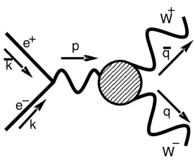
Figure 1: The $s$-channel amplitude of the $e^{+}e^{-}\rightarrow W^{+}W^{-}$ process.

Figure 2: The statistical errors of $\alpha_{2}$ and $\alpha_{3}$ for $\Delta\chi^{2}=4$ at the future $e^{+}e^{-}$ collider with $\sqrt{s}=$500GeV and 1000GeV.

We are now ready to discuss the $e^{+}e^{-}\rightarrow W^{+}W^{-}$ process. The corresponding amplitude can be written as

$${\cal M}(e^{+}e^{-}\rightarrow W^{+}W^{-})={\cal M}_{S}+{\cal M}_{T},$$ (14)

with ${\cal M}_{S}$ and ${\cal M}_{T}$ being $s$-channel and $t$-channel amplitudes respectively. The $s$-channel amplitude can be written as (see Fig.2)

$${\cal M}_{S}=e_{*}^{2}\gamma^{\mu}Q\frac{1}{-p^{2}}\Gamma_{\mu\alpha\beta}^{\gamma*}+\frac{e_{*}^{2}}{s_{*}^{2}}\gamma^{\mu}(I_{3}-s_{*}^{2}Q)\frac{1}{-p^{2}+M_{Z*}^{2}}\Gamma_{\mu\alpha\beta}^{Z*}.$$ (15)

The $WWV$ vertices, $\Gamma_{\mu\alpha\beta}^{\gamma*}$ and $\Gamma_{\mu\alpha\beta}^{Z*}$, can be expressed in terms of the form factors^?:

$$\Gamma_{\mu\alpha\beta}^{V*} = f_{1}^{V*}(q-\bar{q})_{\mu}g_{\alpha\beta}-f_{2}^{V*}(q-\bar{q})_{\mu}p_{\alpha}p_{\beta}+f_{3}^{V*}(p_{\alpha}g_{\mu\beta}-p_{\beta}g_{\mu\alpha})$$ (16)

$$+if_{5}^{V*}\epsilon_{\mu\alpha\beta\rho}(q-\bar{q})^{\rho}.$$

The form factors $f_{3}^{\gamma}$, $f_{1}^{Z}$, $f_{3}^{Z}$ and $f_{5}^{Z}$ depend on the chiral coefficients $\alpha_{1,2,3,8,9,11}$,

$$f_{3}^{\gamma*} = f_{3}^{\gamma*}{}_{\rm SM}+\frac{e^{2}}{s^{2}}(-\hat{\alpha}_{1}+\hat{\alpha}_{2}+\hat{\alpha}_{3}-\hat{\alpha}_{8}+\hat{\alpha}_{9}),$$ (17)

$$f_{1}^{Z*} = f_{1}^{Z*}{}_{\rm SM}+\frac{e^{2}}{s^{2}c^{2}}\hat{\alpha}_{3},$$ (18)

$$f_{3}^{Z*} = f_{3}^{Z*}{}_{\rm SM}+\frac{e^{2}}{s^{2}c^{2}}\hat{\alpha}_{3}+\frac{e^{2}}{c^{2}}(\hat{\alpha}_{1}-\hat{\alpha}_{2})+\frac{e^{2}}{s^{2}}(\hat{\alpha}_{3}-\hat{\alpha}_{8}+\hat{\alpha}_{9}),$$ (19)

$$f_{5}^{Z*} = f_{5}^{Z*}{}_{\rm SM}+\frac{e^{2}}{s^{2}c^{2}}\hat{\alpha}_{11},$$ (20)

while $f_{1}^{\gamma}$, $f_{2}^{\gamma}$, $f_{5}^{\gamma}$ and $f_{2}^{Z}$ do not receive non-decoupling effects from heavy particles. The $\ln M_{H}$ dependence cancels between $f^{V*}_{i,{\rm SM}}$ and $\hat{\alpha}_{i}$. The remaining $M_{H}^{2}$ dependence in $f^{*}_{SM}$ is suppressed by $1/M_{H}^{2}$.

In a similar manner, the $t$-channel neutrino exchange amplitude is given by:

$${\cal M}_{T}=\frac{e_{*}^{2}(t)}{s_{W*}^{2}(t)}\gamma_{\alpha}\frac{1-\gamma_{5}}{2}\frac{1}{\hbox to0.0pt{\hbox to5.00002pt{\hfil$q$\hfil}\hss}/-\hbox to0.0pt{\hbox to5.52084pt{\hfil/\hfil}\hss}k}\gamma_{\beta},\qquad t\equiv(q-k)^{2},$$ (21)

with $s_{W*}(t)$ being

$$s^{2}_{W*}(t)=s^{2}_{W*}(t)_{\rm SM}+e^{2}(\hat{\alpha}_{1}+\hat{\alpha}_{8}).$$ (22)

We are now ready to evaluate the sensitivity limit to these chiral coefficients of the $e^{+}e^{-}\rightarrow W^{+}W^{-}$ differential cross section. The angular distribution can be measured from the decay $WW\rightarrow\ell\nu,q\bar{q}$, which has a 28% branching fraction. We use the differential cross section in the range $-0.8<\cos\theta<0.8$. A detection efficiency of 50% is assumed for the decay $WW\rightarrow\ell\nu,q\bar{q}$.

In the sensitivity limit calculation, we can neglect the SM loop contribution in the running of the form factors. We also neglect the uncertainty of the SM input parameters. As a set of input parameters of the SM we use ($M_{Z}=91.19$GeV, $4\pi/e^{2}_{*}(M_{Z}^{2})=128.72$, $s^{2}_{*}(M_{Z}^{2})=0.2305$).

Fig.2 shows the sensitivity ($\Delta\chi^{2}=\chi^{2}-\chi^{2}_{\rm min}<4$) to the chiral coefficients $\alpha_{2,3}$ as functions of the integrated luminosity of a future $e^{+}e^{-}$ collider. When making the graph of $\Delta\alpha_{2}$ ($\Delta\alpha_{3}$), we assumed that all chiral coefficients other than $\alpha_{2}$ ($\alpha_{3}$) are zero. We discuss physical meaning of this sensitivity in the next section.

4 A model of techni-$\rho$ like resonance

We next evaluate the size of the chiral coefficients $\alpha_{1,2,3,8,9,11}$ predicted in a techni-$\rho$ like vector resonance model. For such a purpose we first construct a phenomenological Lagrangian of the vector resonance.

One of the most familiar chiral Lagrangian formulations of the vector resonance is the hidden local symmetry formalism^?. The usual phenomenological Lagrangian with hidden local symmetry contains two independent parameters, $a$ and $g$. The techni-$\rho$ like resonance has three independent observable quantities when it is on-shell (total decay width, fermionic decay width, and its mass). We thus need to generalize the hidden local symmetry Lagrangian:

$${\cal L}=v^{2}\mbox{tr}(\hat{\alpha}_{\mu\perp}\hat{\alpha}^{\mu}_{\perp})+av^{2}\mbox{tr}(\hat{\alpha}_{\mu\parallel}\hat{\alpha}^{\mu}_{\parallel})-\frac{1}{2g^{2}}\mbox{tr}(V_{\mu\nu}V^{\mu\nu})+\frac{z_{4}}{2}i\mbox{tr}(V_{\mu\nu}[\hat{\alpha}^{\mu}_{\perp},\hat{\alpha}^{\nu}_{\perp}]),$$ (23)

where $V_{\mu}$ stands for the techni-$\rho$ resonance field. The Maurer-Cartan one forms $\hat{\alpha}_{\mu\perp}$ and $\hat{\alpha}_{\mu\parallel}$ are defined by

$$\hat{\alpha}_{\mu\perp}=\frac{1}{2i}\left[D_{\mu}\xi_{L}\cdot\xi_{L}^{\dagger}-D_{\mu}\xi_{R}\cdot\xi_{R}^{\dagger}\right],\qquad\hat{\alpha}_{\mu\parallel}=\frac{1}{2i}\left[D_{\mu}\xi_{L}\cdot\xi_{L}^{\dagger}+D_{\mu}\xi_{R}\cdot\xi_{R}^{\dagger}\right],$$ (24)

with $\xi_{L}$, $\xi_{R}$ from $U=\xi_{L}^{\dagger}\xi_{R}$. The covariant derivative $D_{\mu}$ is given by

$$D_{\mu}\xi_{L}=\partial_{\mu}\xi_{L}-iV_{\mu}\xi_{L}-ig_{2}\xi_{L}W_{\mu}^{a}\frac{\tau^{a}}{2},\qquad D_{\mu}\xi_{R}=\partial_{\mu}\xi_{R}-iV_{\mu}\xi_{R}-ig_{Y}\xi_{R}B_{\mu}\frac{\tau^{3}}{2}.$$ (25)

In addition to the usual parameters of the hidden local symmetry Lagrangian, $a$ and $g$, we introduced one additional parameter, $z_{4}$, which parametrizes the non-minimal coupling of the vector resonance. We can show the equivalence of this formulation with the anti-symmetric tensor formulation.^? The relation to the BESS model will be clarified elsewhere^?.

The mass of the techni-$\rho$ resonance is given by

$$M_{V}^{2}=g^{2}av^{2}.$$ (26)

In the QCD-like technicolor model, vector meson dominance and the KSRF relation^? lead to the parameters

$$a=2,\qquad z_{4}=0.$$ (27)

We next consider the matching of the electroweak chiral Lagrangian of Eq.(5) with the phenomenological vector resonance model Eq.(23). We assume that the tree level matching conditions can be applied at the scale of the techni-$\rho$ resonance,

$$\alpha_{1}^{r}(\mu=M_{V}) = -\frac{av^{2}}{4M_{V}^{2}},$$ (28)

$$\alpha_{2}^{r}(\mu=M_{V}) = \alpha_{3}^{r}(\mu=M_{V})=-\frac{av^{2}}{8M_{V}^{2}}+\frac{z_{4}}{16}.$$ (29)

This assumption is known to work well in the case of the low energy pion chiral Lagrangian^?.

Subtracting the SM contribution of Eqs.(8)–(9) from Eqs.(28)–(29), we find

$$\hat{\alpha}_{1} = -\frac{av^{2}}{4M_{V}^{2}}+\frac{1}{12(4\pi)^{2}}\left[\frac{11}{6}-\ln\left(\frac{M_{V}^{2}}{M_{H}^{2}}\right)\right],$$ (30)

$$\hat{\alpha}_{2} = \hat{\alpha}_{3}=-\frac{av^{2}}{8M_{V}^{2}}+\frac{z_{4}}{16}-\frac{1}{24(4\pi)^{2}}\left[\frac{11}{6}+\ln\left(\frac{M_{V}^{2}}{M_{H}^{2}}\right)\right],$$ (31)

$$\hat{\alpha}_{8} = \hat{\alpha}_{9}=\hat{\alpha}_{11}=0.$$ (32)

The logarithmic correction $\ln(M_{V})$ is due to the renormalization group evolution of the chiral coefficients below the mass of the techni-$\rho$ resonance.

Since the techni-$\rho$ resonance contributes both to $\alpha_{1}$ and to $\alpha_{2}=\alpha_{3}$, we need to calculate the limit contour in the $\alpha_{1}$–($\alpha_{2}=\alpha_{3}$) plane. The limit contour for $\Delta\chi^{2}=\chi^{2}-\chi^{2}_{\rm min}<4$ is shown in Fig.4 for $\sqrt{s}=500$GeV and an integrated luminosity of $\int{\cal L}=100$fb^-1 assuming $\chi^{2}_{\rm min}$ corresponds to the SM with $M_{H}=1$TeV. In Fig.4 the techni-$\rho$ contribution Eqs.(30)–(31) for a QCD-like technicolor model $a=2,z_{4}=0$ is also depicted. The limit of Fig.4 corresponds to $M_{V}\mathop{>}\limits_{\displaystyle{\sim}}3$TeV for the QCD-like techni-$\rho$ resonance. We summarize in Fig.4 the sensitivity to the techni-$\rho$ resonance for the generalized parameter space of the vector resonance model.

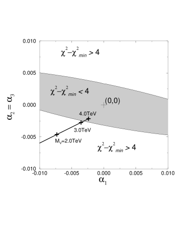
Figure 3: The statistical errors in the $\alpha_{1}$–$(\alpha_{2}=\alpha_{3})$ plane for $\Delta\chi^{2}=4$ at a future $e^{+}e^{-}$ collider with $\sqrt{s}=$500GeV and $\int{\cal L}=100$fb^-1. The techni-$\rho$ contribution is also depicted for the QCD-like technicolor model.

Figure 4: The vector resonance mass lower bound obtained from the electroweak chiral coefficients. The region above the curves is excluded. Constraints including the decoupling effects are also shown.

So far we have considered non-decoupling effects and neglected the decoupling corrections. We need to be careful for the case of a light vector resonance, however, since decoupling effects may play an important role. For such a purpose we calculate the form factors in the techni-$\rho$ resonance model without making the momentum expansion. Fig.4 shows the sensitivity limit calculated from these form factors including the decoupling corrections. We find that the decoupling effects are negligible over a wide range of parameters.

We note that the uncertainties of the SM input parameters and the luminosity measurements are neglected in this talk. We should also combine our analysis with LEP/SLC precision measurements for a detailed study. The analysis with respect to these problems will be published elsewhere^?.

5 Summary

We have determined the sensitivity of the $e^{+}e^{-}\rightarrow W^{+}W^{-}$ at a future $e^{+}e^{-}$ linear collider to non-decoupling effects (electroweak chiral coefficients). The renormalization scale independent electroweak chiral coefficients are defined by subtracting the SM contributions. The effect of one loop chiral logarithms can be taken into account in this definition of the chiral coefficients. A future $e^{+}e^{-}$ collider with $\sqrt{s}=500$GeV, $\int{\cal L}=100$fb^-1 can measure these chiral coefficients up to the statistical errors $\Delta\alpha_{2}\simeq 0.01$ and $\Delta\alpha_{3}\simeq 0.005$ for $\Delta\chi^{2}=4$.

The sensitivity to the techni-$\rho$ like resonance can be extracted from this analysis. The estimated statistical error in the $\hat{\alpha}_{1}$–($\hat{\alpha}_{2}=\hat{\alpha}_{3}$) plane corresponds to a sensitivity to a techni-$\rho$ with a mass $M_{V}\simeq 3$TeV for the QCD-like technicolor model assuming that the $\chi^{2}_{\rm min}$ corresponds to the SM with $M_{H}=1$TeV. The decoupling effects of the vector resonance are also investigated and found to be negligible over a wide range of parameters.

References

References

- [1] S. Weinberg, Physica 96A (1979) 327.
- [2] J. Gasser and H. Leutwyler, Ann. Phys. (N.Y.) 158 (1984) 142; Nucl. Phys. B250 (1985) 465.
- [3] G. Ecker, J. Gasser, H. Leutwyler, A. Pich and E. de Rafael, Phys. Lett. B223 (1989) 425. See also G. Ecker, J. Gasser, A. Pich and E. de Rafael, Nucl. Phys. B321 (1989) 311; J.F. Donoghue, C. Ramirez and G. Valencia, Phys. Rev. D39 (1989) 1947.
- [4] B. Holdom, Phys. Lett. B258 (1991) 156.
- [5] A.F. Falk, M. Luke, E.H. Simmons, Nucl. Phys. B365 (1991) 523.
- [6] For a review, see J. Wudka, Int.J.Mod.Phys. A9 (1994) 2301.
- [7] For a recent detailed analysis, see A.A. Likhoded, T. Han and G. Valencia, hep-ph/9511298.
- [8] T. Barklow, in Proceedings of the Workshop on Physics and Experiments with Linear Colliders, April 26–30 1993, Saariselkaä, Finland, eds. R. Orava et al., (World Scientific, Singapore, 1992).
- [9] A. Miyamoto, K. Hikasa, T. Izubuchi, in Proceedings of INS Workshop Physics of , and Collisions at Linear Accelerators, Dec 20–22, 1994, INS, Tokyo.
- [10] K. Hikasa, T. Izubuchi, A. Miyamoto and M. Tanabashi, in preparation.
- [11] R. Casalbuoni, S. De Curtis, D. Dominici, P. Chiappetta, A. Deandrea and R. Gatto, in Proceeding of the Workshop on Physics and Experiments with Linear Colliders, April 26–30 1993, Waikoloa, Hawaii, eds. F. Harris et al., (World Scientific, Singapore, 1993).
- [12] R. Casalbuoni, S. De Curtis, D. Dominici and R. Gatto, Phys. Lett. B155, (1985) 95; Nucl. Phys. B282, (1987) 235.
- [13] A. Longhitano, Phys. Rev. D22 (1980) 1166; Nucl. Phys. B188 (1981) 118.
- [14] T. Appelquist and G-H. Wu, Phys. Rev. D48 (1993) 3235.
- [15] M. E. Peskin and T. Takeuchi, Phys. Rev. Lett. 65 (1990) 964; B. Holdom and J. Terning, Phys. Lett. B247 (1990) 88.
- [16] See for example, A. Miyamoto, these Proceedings.
- [17] D.C. Kennedy and B.W. Lynn, Nucl. Phys. B322 (1989) 1.
- [18] K. Hagiwara, R.D. Peccei, D. Zeppenfeld and K. Hikasa, Nucl. Phys. B282 (1987) 253.
- [19] M. Bando, T. Kugo, S. Uehara, K. Yamawaki and T. Yanagida, Phys. Rev. Lett. 54 (1985) 1215; For a review, see M. Bando, T. Kugo and K. Yamawaki, Phys. Reports 164 (1988) 218.
- [20] M. Tanabashi, KEK-TH-438, hep-ph/9511367. See also J. Bijnens and E. Pallante, NORDITA-95/63 N,P, hep-ph/9510338.
- [21] K. Kawarabayashi and M. Suzuki, Phys. Rev. Lett. 16 (1966) 255; Riazuddin and Fayyazuddin, Phys. Rev. 147 (1966) 1071.