Computational Study of Baryon Number Violation
in High Energy Electroweak Collisions

Abstract

We use semiclassical methods to study processes which give rise to change of topology and therefore to baryon number violation in the standard model. We consider classically allowed processes, i.e. energies above the sphaleron barrier. We develop a computational procedure that allows us to solve the Yang Mills equations of motion for spherically symmetric configurations and to identify the particle numbers of the in- and out-states. A stochastic sampling technique is then used to map the region spanned by the topology changing solutions in the energy versus incoming particle number plane and, in particular, to determine its lower boundary. A lower boundary which approaches small particle number would be a strong indication that baryon number violation would occur in high energy collisions, whereas a lower asymptote at large particle number would be evidence of the contrary. With our method and the computational resources we have had at our disposal, we have been able to determine the lower boundary up to energies approximately equal to one and a half time times the sphaleron energy and observed a 40% decrease in particle number with no sign of the particle number leveling off. However encouraging this may be, the decrease in incoming particle number is only from 50 particles down to approximately 30. Nevertheless, the formalism we have established will make it possible to extend the scope of this investigation and also to study processes in the classically forbidden region, which we plan to do in the future.

BUHEP-95-33 Submitted to Physical Review D

hep-ph/9601260 Typeset in REVTeX

I Introduction

Since the pioneering work of   ’t Hooft[1] it has been known that the axial vector anomaly implies that baryon number is not conserved in processes which change the topology of the gauge fields. Baryon number violating amplitudes are non-perturbative and viable methods of calculation are scarce. The two primary methods of obtaining non-perturbative information in quantum field theory are either semi-classical techniques or direct lattice simulations of the quantum fluctuations. Theories with small coupling constants are not suited for the latter, so the electroweak sector of the standard model lies beyond the reach of direct lattice calculations. This means that semiclassical methods presently offer the only way to study baryon number violating electroweak processes.

Electroweak baryon number violation is associated with topology change of the gauge fields. Classically, gauge field configurations with different topology (i.e. differing by a topologically non-trivial gauge transformation) are separated by an energy barrier. The (unstable) static solution of the classical equations of motion which lies at the top of the energy barrier is called the sphaleron[2]. At energies lower than the sphaleron energy, topology changing transitions, and hence baryon number violation, can only occur via quantum mechanical tunneling. At zero temperature and low energy the tunneling rate can be reliably calculated and is exponentially small. A few years ago, however, Ringwald [3] and Espinosa[4] noticed that a summation of the semiclassical amplitudes over final states gives rise to factors which increase very rapidly with increasing energy. This may lead to a compensation of the exponential suppression for energies approaching the energy of the barrier, i.e. the sphaleron energy $E_{\rm sph}$. Intuitively, one might expect suppression of tunneling to become much less severe as the energy approaches the energy of the barrier, in particular, one might expect it to disappear altogether for $E>E_{\rm sph}$, i.e. in the region where the topology changing processes are classically allowed. Investigations have indeed confirmed that this is precisely what happens in high temperature electroweak processes[5]: as the temperature approaches $E_{\rm sph}$ (which is in fact temperature dependent for a thermal plasma), the barrier-penetration suppression factor becomes progressively less pronounced, and electroweak baryon number violation becomes unsuppressed altogether above the critical temperature. The situation is, however, much less clear for high energy collisions and it would be premature to conclude that baryon number violation can occur with a non-negligible amplitude. Phase space considerations are more subtle and simply because one has enough energy to pass over the barrier does not guarantee that one does so. The problem is that in high energy collisions the incident state is an exclusive two particle state, which is difficult to incorporate in a semiclassical treatment of the transition amplitude.

A possible remedy to this situation has recently been proposed by Rubakov, Son and Tinyakov[6] who suggested that one considers incident coherent states, but constrained so that energy and particle number take fixed average values

$$E = {\epsilon\over g^{2}}$$ (2)

$$N = {\nu\over g^{2}}.$$ (3)

In the limit $g\to 0$, with $\epsilon$ and $\nu$ held fixed, the path integrals giving the transition amplitudes are then dominated by a saddle point configuration which solves the classical equations of motion. This permits a semiclassical calculation of the transition rates. Information on high energy collision processes with small numbers of incident particles can then be obtained from the limit $\nu\to 0$. While this limit does not strictly reproduce the exclusive two-particle incoming state, under some reasonable assumptions of continuity it can be argued that the corresponding transition rates will be equally suppressed or unsuppressed.

When the energy is below the sphaleron barrier the semiclassical paths that dominate the functional integral in Ref. [6] must be complex for (I) to be satisfied. Finding such solutions is a formidable analytic problem, but one that is well suited to numerical study. The numerical evolution naturally divides into two regimes. There is a purely Euclidean evolution, corresponding to tunneling under the barrier, and a Minkowski evolution corresponding to classical motion before and after the tunneling event. The desired semiclassical paths may be obtained by appropriately matching the Euclidean and Minkowski solutions onto one another, and the transition amplitude may then be calculated.

When the energy is greater than the sphaleron barrier, transitions are classically allowed and solutions that saturate the functional integral are real. This is the regime examined in this paper. When chiral fermions are coupled to gauge and Higgs fields which undergo topological transitions, Ref. [7] shows that the anomalous fermion number violation is given by the change in Higgs winding number of the classical system. This paper is primarily an investigation of whether and to what extent topology change occurs in classical evolution with low particle number in the incident state. Since Minkowski evolution is also required for the analysis below the sphaleron, the techniques developed in the present investigation will be useful there as well.

The primary impediment for rapid baryon number violation is the phase space mismatch between incoming states of low multiplicity and outgoing states of many particles. The authors of Ref. [8] look at simplified models and observe that, classically, it is difficult to transfer energy from a small number of hard modes to a large number of soft modes. However, the investigations in Ref. [9] find that for pure Yang-Mills theory in 2-dimensions the momenta can be dramatically redistributed, although unfortunately the incident particle number seems to be rather large in their domain of applicability. Ref. [10] studies the Yang-Mills-Higgs system in a 2-dimensional plane-wave Ansatz and again finds that momentum can be efficiently redistributed. It is the purpose of our investigation to shed further light on the situation in 4-dimensions in the presence of a Higgs field and to investigate the relation between incoming particle number and topology change.

Given a typical classical solution, because of the dispersion of the energy, the fields will asymptotically approach vacuum values. Consequently, at sufficiently early and late times the field equations will reduce to linearized equations describing small oscillations about the vacuum and the field evolution will be a superposition of normal mode oscillations. In terms of the frequencies $\omega_{n}$ and amplitudes $a_{n}$ of these oscillators the energy and particle number of (I) are given by

$$\epsilon = \sum_{n}\omega_{n}|a_{n}|^{2}$$ (5)

$$\nu = \sum_{n}|a_{n}|^{2}\ ,$$ (6)

and we see that for typical classical evolution the energy $\epsilon$ and the particle numbers $\nu_{i}$ and $\nu_{o}$ of the asymptotic incoming and outgoing states are well defined (the energy is of course conserved and well defined even in the non-linear regime, although no longer given by (5)). In addition, since the fields approach vacuum values for $t\to\pm\infty$, the winding numbers of incoming and outgoing configurations are also well defined. Because of the sphaleron barrier, the energy $\epsilon$ of all the classical solutions with a net change of winding number is bounded below by the sphaleron energy $\epsilon_{\rm sph}$. The problem we would like to solve then is whether the incoming particle number $\nu_{i}$ of these solutions can be arbitrarily small, or more generally, we would like to map the region spanned by all possible values of $\epsilon$ and $\nu_{i}$ for topology changing classical evolution.

One could easily parameterize an initial configuration of the system consisting of incoming waves in the linear regime; however, it would be extremely difficult to adjust the parameters to insure that a change of winding number occurs in the course of the subsequent evolution. For this reason we will instead parameterize the configuration of the system at the moment when a change of topology occurs (this will be our starting configuration), and we will then evolve the equations of motion backward in time. Following the time reversed evolution until the system reaches the asymptotic linear regime allows us to identify the incident particle number $\nu_{i}$. By varying the parameters of the starting configuration with a suitable stochastic procedure we will then be able to map the boundary of the region of topology changing solutions in the $\epsilon$-$\nu$ plane.

Note that the problem of baryon number violation above the barrier may roughly be divided into two parts. One must find the set of incoming coherent states which give rise to a change in topology of the fields, and one must calculate the overlap between the incident two-particle scattering state and such coherent states. Both are very challenging. The problem considered in this paper is the more fundamental of the two, in the sense that if topology change cannot occur for coherent states with small average particle number, the overlap effect with a two particle beam is a moot point. On the other hand, if a change of topology can be induced with arbitrarily low particle number in the incoming state, one is at the very least assured that exponential suppression, which is a residual of the barrier penetration, will be absent.

In summary, then, our strategy is the following. We start with a (not necessarily small) perturbation about the sphaleron with some energy $\epsilon$. We evolve the configuration until it reaches the linear regime, at which time we extract the normal mode amplitudes $a_{n}$ and compute the asymptotic particle number $\nu$. The time reversed solution will have an incident particle number $\nu$ and will typically undergo topology change, since by construction it will pass over the sphaleron barrier. There is of course the possibility that the system will go back over the sphaleron barrier and return to the original topological sector, but we check against this occurrence by evolving the starting configuration in the opposite direction in time and measuring the winding number of the asymptotic state. We can then explore the space of topology changing solutions by varying the parameters of the starting configuration using suitable stochastic techniques. This permits us to map the allowed $\epsilon$-$\nu$ plane in an attempt to place a reliable lower bound on the incident particle number. If this bound is comparable with two particles in the incoming state, it would be an indication that the time reversed solution, which passes over the sphaleron barrier, can be excited in a high energy collision. Hence, this would be a signal that baryon number violation becomes unsuppressed. Likewise, if the bound is large this would indicate that high energy baryon number violation is unobservable in a two-particle scattering experiment.

In what follows we put meat on the bones of the above discussion and present our numerical results. The structure of this paper is as follows. In Section II we illustrate the general properties of sequences of topology changing field configurations, not necessarily solutions to the equations of motion. For simplicity we first consider the 2-dimensional Abelian Higgs model. We then examine the 4-dimensional $SU(2)$ Higgs model, but restricted to the spherical Ansatz to obtain a computationally tractable system. In Section III we examine the classical evolution in the continuum. Since the field equations are coupled non-linear partial differential equations, in Section IV we solve them by numerical techniques. In Section V we describe the starting configurations at the moment of topology change, i.e. our parameterization of the initial state, and in Section VI we solve the normal mode problem necessary for extracting the particle number in the linear regime. In Section VII we explain the stochastic sampling technique used to probe the initial configuration space and we present our numerical results concerning the region spanned in the $\epsilon$-$\nu$ plane by topology changing solutions. In Section VIII we present concluding remarks and directions for future research. The reader who is familiar with the the basic properties of the $SU(2)$ Higgs system and of topology changing solutions, and is impatient to learn about our results, may skip directly to Section VII. However, in our opinion, much of the value of the research we present here is to be found in the formalism we have established to parameterize, evolve and analyze classical solutions of the $SU(2)$ Higgs system in the spherical Ansatz. This formalism, which is illustrated in Sections II through VI, has not only been crucial for obtaining our current results, but we are confident it will be invaluable for further investigation into the problem of collision-induced baryon number violation both above and below the sphaleron barrier.

II Topology Changing Sequences of Configurations

We start our investigation with the 1+1 dimensional Abelian Higgs system, which is defined in terms of a complex scalar field $\phi(x)$ and an Abelian gauge potential $A_{\mu}(x)$ with action

$$S=\int dx^{2}~{}\left\{-{1\over 4}F_{\mu\nu}F^{\mu\nu}+D_{\mu}\phi^{*}D^{\mu}\phi-\lambda(|\phi|^{2}-1)^{2}\right\}\ ,$$ (7)

where the indices run over 0 and 1, $F_{\mu\nu}=\partial_{\mu}A_{\nu}-\partial_{\nu}A_{\mu}$ and $D_{\mu}\phi=\partial_{\mu}\phi-iA_{\mu}\phi$. We have set the coupling constant $g=1$ and several inessential constants have been eliminated by a suitable choice of units.

The most important feature of this system is that the vacuum, i.e. the configuration of minimum energy, occurs for non-vanishing $\phi$, indeed, in our units for $|\phi|=1$. Since this does not specify the phase of $\phi$, there is not a unique vacuum state, but rather multiple vacua. Still, because of gauge invariance one must be careful in regard to the physical significance of the phase of $\phi$. A local variation in the phase of $\phi$ can always be undone by a suitable gauge transformation, and since gauge equivalent configurations must be considered physically indistinguishable, local variations of the phase of the scalar field do not lead to different vacua. However, variations of the phase of $\phi$ by multiples of $2\pi$ (as the coordinate $x^{1}$ spans the entire spatial axis) cannot be undone by a local gauge transformation, and thus define topologically distinct vacuum states. These vacua differ by the global topological properties of the field configuration. The condition $|\phi|=1$ restricts the values of the scalar field to the unit circle (in the complex plane). In the $A_{0}=0$ gauge, which we use throughout this paper, the values assumed by $\phi$ at $x^{1}=\pm\infty$ stay constant in time. If we demand that $\phi$ takes fixed identical values as $x^{1}\to\pm\infty$ (a condition we later relax), then the number of times $\phi$ winds around the unit circle as $x^{1}$ spans the entire real axis is a topological invariant (the winding number) which characterizes different topologically inequivalent vacuum states.

FIG. 1.: Example of two inequivalent vacuum configurations (a, c) and a field configuration at the top of the energy barrier separating them (b). Figures a, b and c trace the field $\phi$ in the complex plane as the spatial coordinate spans the entire axis. A three dimensional perspective has been added in figures d, e and f to illustrate the detailed dependence of $\phi$ on the spatial coordinate.

Figures 1a-c illustrate three possible contours traced in the complex plane by the field variable $\phi(x^{1})$ as the coordinate $x^{1}$ spans the entire space axis. Inequivalent vacuum configurations with winding numbers 0 and 1 respectively are depicted in Figs. 1a and 1c. In the contour of Fig. 1a the phase of $\phi$ stays fixed at zero as $x^{1}$ ranges between $-\infty$ and $+\infty$, whereas it goes once around the unit circle in Fig. 1c. Consequently, the corresponding vacuum configurations have winding numbers $0$ and $1$. The detailed variation of the phase is immaterial since it can always be changed locally by a gauge transformation. Thus, in Fig. 1a for example, as $x$ varies from $-\infty$ to $+\infty$ the field does not have to stay fixed, but could wander continuously on the unit circle provided the net change in phase is zero. However, the configuration of Fig. 1a cannot be continuously deformed to that of Fig. 1c without leaving the vacuum manifold. Therefore a continuous path of configurations connecting neighboring vacua must pass over an energy barrier, a configuration which has the property that $\phi$ vanishes at a point, rendering its phase there undefined. The smallest such energy barrier is called the sphaleron[2], and its Higgs field component is illustrated in Fig. 1b. Figures  1d-f add the additional perspective of spatial dependence for the field $\phi(x^{1})$. Figures 1a-c can be viewed as projections onto the complex plane orthogonal to the $x^{1}$ axis of the curves in Figs. 1d-e.

FIG. 2.: A different gauge equivalent representation of the configurations illustrated in Fig. 1.

One should note that the periodic boundary conditions on $\phi$ at $x^{1}=\pm\infty$ can be relaxed. Sometimes it is convenient to use the freedom of performing a time independent gauge transformation to make $\phi(\infty)$ and $\phi(-\infty)$ differ while keeping both fixed in time (for solutions, the constancy in time of $\phi(\pm\infty)$ follows from the equations of motion in the $A_{0}=0$ gauge). Thus, the configurations of Figs. 1a-c can be gauge transformed into the configurations shown in Figs. 2a-c. In Fig. 2a the phase of $\phi$ changes by $-\pi$ as $x^{1}$ goes from $-\infty$ to $+\infty$, while in Fig. 2c it rotates by $\pi$. As in Fig. 1, the two vacuum configurations differ by a phase rotation of $2\pi$, i.e. by a unit change of winding number. In the intermediate configuration (Fig. 2b) the scalar field takes only imaginary values. In this gauge the sphaleron configuration takes a very simple form

$$\phi(x^{1})=i\tanh[\sqrt{\lambda}\,(x^{1}-c)],\quad A_{\mu}=0,$$ (8)

where $c$ specifies the location of the sphaleron.

A possible parameterization for the entire evolution illustrated in Fig. 2 can be conveniently written as

$$\phi(x^{1}) = i{1-\exp[i\tau-2\sqrt{\lambda}\,(x^{1}-c)]\over 1+\exp[i\tau-2\sqrt{\lambda}\,(x^{1}-c)]}$$ (10)

$$A_{1} = {4\tau\sqrt{\lambda}\over\pi\cosh[2\sqrt{\lambda}\,(x^{1}-c)]}\ ,$$ (11)

with $A_{0}=0$. As the reader can easily verify, for $\tau=-\pi/2$ and $\tau=\pi/2$ the field $\phi$ reduces to a number of unit modulus precisely spanning the contours of Fig. 2a and Fig. 2c respectively (as $x^{1}$ ranges from $-\infty$ to $+\infty$). The corresponding values of $A_{1}$ are chosen to make the gauge covariant derivative of $\phi$ vanish, thus ensuring vacuum. We should point out, however, that (2) does not represent the solution of any particular set of equations of motion (Euclidean or Minkowski). It is merely a compact parameterization of interpolating configurations, in terms of two variables $c$ and $\tau$, which might be useful in studying sphaleron transitions based on the method of collective coordinates.

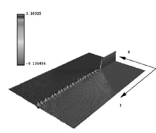
Classical solutions of the 2-dimensional Abelian Higgs model can exhibit topology change in much the same way as the vacuum-to-vacuum paths described above. If one couples chiral fermions to the system, the fermionic current has an anomaly which leads to fermion number violation in the presence of topology changing classical solutions. Therefore, this model would appear to be a very convenient system for a simplified study of baryon number violation in high energy processes. However, as we will discuss in a future section, a crucial component of the computational investigation is the ability to identify numerically the normal mode amplitudes of the fields in the asymptotic linear regime. No matter how non-linear the system may be at any given point in its classical evolution, typically the energy will disperse and bring the system to a regime where the fields undergo small oscillations about a vacuum configuration. This dispersion is expected to occur in any field theoretical system, unless prevented by conservation laws such as those underlying soliton phenomena. Now, while the 2-dimensional Abelian Higgs model does not possess soliton solutions, we have observed computationally that the decay of the sphaleron in this system nevertheless gives origin to persistent, localized, large oscillations with an extremely small damping rate (this observation was also made by Arnold and McLerran in Ref. [12]). These oscillations, illustrated in Fig. 3, make the system quite unwieldy for a computational investigation of baryon number violation based on semiclassical techniques. Consequently we turn our attention to the more realistic 4-dimensional $SU(2)$ Higgs system.

FIG. 3.: Sphaleron decay in the 2-dimensional Abelian Higgs model: classical evolution of the $\phi$ field. The values of the phase of the complex field are coded by shades of gray, and the modulus of the field by the height of the surface. The sphaleron decays rather quickly, but leaves behind a quasi-stable oscillating remnant. For a full color figure see http://cthulu.bu.edu/$\scriptstyle\sim$bobs/bviolate.html.

Throughout this paper we will ignore both the $U(1)$ hypercharge and the back-reaction of the fermions on the dynamics of the gauge and Higgs fields. We shall examine the 3+1 dimensional $SU(2)$ Higgs system, which is defined in terms of a complex doublet $\Phi(x)$ and a gauge potential $A_{\mu}(x)$ with action

$$S=\int dx^{4}~{}\left\{-{1\over 2}{\rm Tr}\,F_{\mu\nu}F^{\mu\nu}+(D_{\mu}\Phi)^{\dagger}D^{\mu}\Phi-\lambda(\Phi^{\dagger}\Phi-1)^{2}\right\}\ ,$$ (12)

where the indices run from $0$ to $3$ and where

$$F_{\mu\nu} = \partial_{\mu}A_{\nu}-\partial_{\nu}A_{\mu}-i[A_{\mu},A_{\nu}]$$ (13)

$$D_{\mu}\Phi = (\partial_{\mu}-iA_{\mu})\Phi$$ (14)

with $A_{\mu}=A^{a}_{\mu}\sigma^{a}/2$. We use the standard metric $\eta_{\mu\nu}={\rm diag}(1,-1,-1,-1)$, and we have eliminated several inessential constants by a suitable choice of units. We have also set the coupling constant $g=1$, but shall restore it when explicitly needed using the standard model value $g=0.652$. For our numerical investigation we shall take the Higgs self-coupling $\lambda=0.1$, which corresponds to $m_{\rm H}=110{~{}\rm GeV}$. This value of $\lambda$ is small enough that Higgs-field dynamics is non-trivial, but large enough to allow many lattice sites to fall within a single Higgs Compton wave length.

Because of the larger dimensionality of space one expects the energy to disperse much more readily in this system than in the 1+1 dimensional Abelian Higgs model, an expectation borne out by results of Hellmund and Kripfganz[13] who observed the onset of a linear regime following the sphaleron’s decay. For a computationally manageable problem, we focus on the spherically symmetric configurations of Ratra and Yaffe[14], which reduce the system to an effective 2-dimensional theory. This effective theory, however, still has much in common with the full 4-dimensional theory, such as possessing similar topological structure. Furthermore, despite its lower dimensionality, we shall see that the effective system still linearizes because of explicit kinematic factors of $r$ in the equations of motion (these factors are lacking for the 1+1 dimensional Abelian Higgs model). The ease of linearization in this effective 2-dimensional theory is physically reasonable since solutions within the spherical ansatz can have their energy distributed over expanding spherical shells.

Explicitly, the spherical Ansatz is given by expressing the gauge and Higgs fields in terms of six real functions $a_{0}\,,\,a_{1}\,,\,\alpha\,,\,\beta\,,\,\mu\ {\rm and}\ \nu\ {\rm of}\ r\ {\rm and}\ t$:

$$A_{0}({\bf x},t) = \frac{1}{2}\,a_{0}(r,t)\mbox{\boldmath$\sigma$}\cdot{\bf\hat{x}}$$ (16)

$$A_{i}({\bf x},t) = \frac{1}{2}\,\big{[}a_{1}(r,t)\mbox{\boldmath$\sigma$}\cdot{\bf\hat{x}}\hat{x}^{i}+\frac{\alpha(r,t)}{r}(\sigma^{i}-\mbox{\boldmath$\sigma$}\cdot{\bf\hat{x}}\hat{x}^{i})+\frac{1+\beta(r,t)}{r}\epsilon^{ijk}\hat{x}^{j}\sigma^{k}\big{]}$$ (17)

$$\Phi({\bf x},t) = [\mu(r,t)+i\nu(r,t)\mbox{\boldmath$\sigma$}\cdot{\bf\hat{x}}]\xi\ ,$$ (18)

where ${\bf\hat{x}}$ is the unit three-vector in the radial direction and $\xi$ is an arbitrary two-component complex unit vector. For the 4-dimensional fields to be regular at the origin, $a_{0}$, $\alpha$, $a_{1}-\alpha/r$, $(1+\beta)/r$ and $\nu$ must vanish like some appropriate power of $r$ as $r\to 0$.

Note that configurations in the spherical Ansatz remain in the spherical Ansatz under gauge transformations of the form

$$A_{\mu} \to A_{\mu}+iU^{\dagger}\partial_{\mu}U~{}~{}~{}~{}~{}~{}\mu=0\cdots 3$$ (19)

$$\Phi\, \to U\Phi\ ,$$ (20)

where the gauge function is given by

$$U=\exp[i\Omega(r,t)\mbox{\boldmath$\sigma$}\cdot{\bf\hat{x}}/2]\ .$$ (21)

We require $\Omega(0,t)=0$ to ensure that gauge transformed configurations of regular fields remain regular at the origin. This spherical gauge degree of freedom induces a residual $U(1)$ gauge invariance in an effective 2-dimensional theory. The action of this effective theory can be obtained by inserting (3) into (12), from which one finds

$$S=4\pi\int dt\int^{\infty}_{0}dr \bigg{[}-\frac{1}{4}r^{2}f^{\mu\nu}f_{\mu\nu}+D^{\mu}\chi^{*}D_{\mu}\chi+r^{2}D^{\mu}\phi^{*}D_{\mu}\phi$$ (24)

$$-\frac{1}{2r^{2}}\left(~{}|\chi|^{2}-1\right)^{2}-\frac{1}{2}(|\chi|^{2}+1)|\phi|^{2}-{\rm Re}(i\chi^{*}\phi^{2})$$

$$-\lambda\,r^{2}\,\left(|\phi|^{2}-1\right)^{2}~{}\bigg{]}\ ,$$

where the indices now run from $0$ to $1$ and in contrast to Ref. [14] are raised and lowered with $\eta_{\mu\nu}={\rm diag}(1,-1)$, and where

$$f_{\mu\nu} = \partial_{\mu}a_{\nu}-\partial_{\nu}a_{\mu}\$$ (25)

$$\chi = \alpha+i\beta$$ (26)

$$\phi = \mu+i\nu\$$ (27)

$$D_{\mu}\chi = (\partial_{\mu}-i\,a_{\mu})\chi$$ (28)

$$D_{\mu}\phi = (\partial_{\mu}-\frac{i}{2}\,a_{\mu})\phi\ .$$ (29)

The action (24) is indeed invariant under the $U(1)$ gauge transformation

$$a_{\mu} \to a_{\mu}+\partial_{\mu}\Omega$$ (31)

$$\chi\, \to e^{i\Omega}\chi$$ (32)

$$\phi\, \to e^{i\Omega/2}\phi\ ,$$ (33)

and we see that the spherical Ansatz effectively yields a system very similar to the Abelian Higgs model considered above. In this reduced system the variables $a_{0}(r,t)$ and $a_{1}(r,t)$ play the role of the 2-dimensional gauge field. The variables $\chi(r,t)$ and $\phi(r,t)$, which parameterize the residual components of the 4-dimensional gauge field and the 4-dimensional Higgs field respectively, both behave as 2-dimensional Higgs fields. Note that $\chi$ has a $U(1)$ charge of one while $\phi$ has charge one half. Of course, the presence of metric factors (powers of $r$) in the action (24) is a reminder that we are really dealing with a 4-dimensional system.

We shall work in the $a_{0}=0$ (or $A_{0}=0$) gauge throughout. In the 4-dimensional theory, if one compactifies 3-space to $S^{3}$ by identifying the points at infinity, it is well known that the vacua correspond to the topologically inequivalent ways of mapping $S^{3}$ into $SU(2)\sim S^{3}$ [15]. These maps are characterized by the third homotopy group of $SU(2)$ and a vacuum can be labeled by an integer called the homotopy index or winding number. The effective 2-dimensional theory inherits a corresponding vacuum structure. From (24) it is apparent that the vacuum states are characterized by $|\chi|=|\phi|=1$, with the additional constraint that $i\chi^{*}\phi^{2}=-1$ (as well as $D_{1}\chi=D_{1}\phi=0$). Convenient zero-winding vacua are given by $\chi_{\rm vac}=-i$, $\phi_{\rm vac}=\pm 1$ with $a_{1\,\rm vac}=0$. There are in fact other vacua with constant fields (and hence zero winding), but from (3) they yield singular 4-dimensional fields. Nontrivial vacua can be obtained from the trivial vacua via the gauge transformation (3):

$$a_{\mu\,\rm vac} = \partial_{\mu}\Omega$$ (35)

$$\chi_{\rm vac}\, = -i\,e^{i\Omega}$$ (36)

$$\phi_{\rm vac}\, = \pm\,e^{i\Omega/2}\ .$$ (37)

When 3-space is compactified $\Omega\to 2n\pi$ as $r\to\infty$ (for non-zero integers $n$). Since $\Omega$ has been set to zero at the origin, the winding numbers of such vacua are simply the integers $n$. Note that $\chi_{\rm vac}$ winds $n$ times around the unit circle while $\phi_{\rm vac}$ only winds by $n/2$. This is because the $\phi$ field has half a unit of $U(1)$ charge while $\chi$ has a full unit. Hence, the phase change of $\chi$ is more dramatic in a topological transition, and for this reason we will often concentrate our attention upon $\chi$ rather than $\phi$, even though the Higgs field is more fundamental for topology change [7].

As will become apparent shortly, it is often convenient to relax the condition that 3-space be compactified. We may then consider vacua (3) for which $\Omega$ does not become an even multiple of $\pi$ at large $r$. In particular, when $\Omega\to(2n+1)\pi$, then $\chi_{\rm vac}\to i$ and $\phi_{\rm vac}\to\pm\,i$ as $r\to\infty$. Then the gauge function $U\to\pm\,i\mbox{\boldmath$\sigma$}\cdot{\bf\hat{x}}$ and becomes direction dependent, and as expected, space cannot be compactified.

As in the Abelian Higgs model a continuous path in the space of all field configurations which interpolates between two inequivalent vacua must necessarily leave the manifold of vacuum configurations and pass over an energy barrier. On such a path there will be a configuration of maximum energy, and of all these maximal energy configurations the sphaleron has the lowest energy and represents a saddle point along the energy ridge separating inequivalent vacua[2]. In the spherical Ansatz we can work in a gauge in which the sphaleron takes a particularly simple form, with $a_{\mu}=0$ and

$$\chi_{\rm sph}(r)=i[2f(r)-1]$$ (38)

$$\phi_{\rm sph}(r)=ih(r)\ ,$$ (39)

where $f$ and $h$ vary between $0$ and $1$ as $r$ changes from $0$ to $\infty$ and are chosen to minimize the energy functional. Note that the $\phi$ field vanishes at the origin and that the $\chi$ field vanishes at some non-zero value of $r$.

This form of the sphaleron, in which the gauge field $a_{\mu}$ vanishes and the fields $\chi$ and $\phi$ are pure imaginary, is convenient for numerical calculations. Nevertheless, it is slightly peculiar in the following sense. Finite energy configurations, like (38), asymptote to pure gauge at spatial infinity (note that $i\chi^{*}_{\rm sph}\phi^{2}_{\rm sph}\to-1$ as $r\to\infty$). Typically a gauge is chosen so that the appropriate gauge function is unity at spatial infinity, and then space can be compactified to the 3-sphere. But (38) gives $\chi_{\rm sph}\to i$ and $\phi_{\rm sph}\to i$, which as we have seen in the discussion following (3) corresponds to the direction dependent gauge function $U\to i\mbox{\boldmath$\sigma$}\cdot{\bf\hat{x}}$. So the sphaleron (38) is in a gauge in which 3-space cannot be compactified. Note that an arbitrary element of $SU(2)$ can be parameterized by ${\rm b}_{0}{\bf 1}+i\mbox{\boldmath$\sigma$}\cdot{\bf b}$ where ${\bf 1}$ is the two by two unit matrix and ${\rm b}_{0}^{2}+{\bf b}^{2}=1$. Hence $SU(2)\sim S^{3}$, and defining the north and south poles by $\pm{\bf 1}$, we see that $i\mbox{\boldmath$\sigma$}\cdot{\bf b}$ with ${\bf b}^{2}=1$ parameterizes the equatorial sphere. Thus the gauge function $U$ maps the sphere at infinity onto the equatorial sphere of $SU(2)$. In this gauge, a topology changing transition proceeding over the sphaleron corresponds to a transition where the fields wind over the lower hemisphere of $SU(2)$ before the transition and over the upper hemisphere after the transition, with a net change in winding number still equal to one. The behavior of the $\chi$ field in a topological transition is then very similar to the behavior of the Higgs field in the 2-dimensional model, already illustrated in Fig. 2. The behavior of the $\phi$ field is illustrated in Fig. 4. We could of course, and sometimes will, work in a gauge consistent with spatial compactification where topological transitions interpolate between vacua of definite winding, as in Fig. 1, but the sphaleron would look more complicated. The advantage of (38) from a computational perspective is that perturbations about the sphaleron can be more easily parameterized.

FIG. 4.: Topological transition in the 4-dimensional $SU(2)$ Higgs model: behavior of the $\phi$ field. The $\chi$ field behaves as in Fig. 2.

III Classical Evolution in the Continuum

So far we have only examined topology changing paths that interpolate between inequivalent vacua. We are now interested in examining the topological structure of solutions to the equations of motion. For vacuum to vacuum sequences it is clear what we mean by topology change: this is simply the change in winding number between the initial and final vacua. For solutions, however, the situation is not quite so straightforward. Nevertheless, topology change can be precisely defined for solutions whose energy density dissipates to zero uniformly in the distant past and future, which is the generic case for classical evolution. In the asymptotic regime the uniform dissipation of energy renders the system linear and the waves can be expressed as small oscillations about vacua of definite winding numbers. By the topology change of such a solution, we simply mean the difference in the winding number between these two asymptotic vacua. This difference in winding is in fact just given by the change in Higgs winding number, and hence is characterized by zeros of the Higgs field (although in the spherical Ansatz it is characterized by zeros of both $\phi$ and $\chi$). The most important physical consequence of this topology change is that when chiral fermions are coupled to the system, fermion number violation occurs and is proportional to the change in winding of the Higgs field (see Ref. [7]).

We wish to study whether topology change, and hence fermion number violation, can occur in the course of classical evolution with small gauge or Higgs particle-number in the incoming state. Since the system we are studying linearizes in the past, the incident particle number is defined and our question is well posed. However, the field equations are coupled non-linear partial differential equations which we cannot solve in closed form. Our approach, then, is to solve the equations numerically with a discretized $r$-axis and discretized time steps, but first it is useful to examine the continuum system.

The equations of motion obtained from the action (24) are

$$\partial^{\mu}(r^{2}f_{\mu\nu})=i\left[D_{\nu}\chi^{*}\chi-\chi^{*}D_{\nu}\chi\right]+\frac{i}{2}\,\,r^{2}\left[D_{\nu}\phi^{*}\phi-\phi^{*}D_{\nu}\phi\right]$$ (41)

$$\left[D^{2}+\frac{1}{r^{2}}(|\chi|^{2}-1)+\frac{1}{2}\,|\phi|^{2}~{}\right]\chi=-\frac{i}{2}\,\,\phi^{2}$$ (42)

$$\left[D^{\mu}r^{2}D_{\mu}+\frac{1}{2}(|\chi|^{2}+1)+2\lambda r^{2}\left(|\phi|^{2}-1\right)\right]\phi=i\,\chi\phi^{*}\ .$$ (43)

To solve these equations given an initial configuration, we must specify the appropriate boundary conditions. Boundary conditions for the fields at $r=0$ can be derived from the requirement that the 4-dimensional configurations they parameterize be regular at the origin. One finds that the behavior as $r\to 0$ must be

$$a_{0} = a_{0,1}r+a_{0,3}r^{3}+\dots$$ (45)

$$a_{1} = a_{1,0}+a_{1,2}r^{2}+a_{1,4}r^{4}+\dots$$ (46)

$$\alpha = \alpha_{1}r+\alpha_{3}r^{3}+\alpha_{5}r^{5}+\dots$$ (47)

$$\beta = -1+\beta_{2}r^{2}+\dots$$ (48)

$$\mu = \mu_{0}+\mu_{2}r^{2}+\dots$$ (49)

$$\nu = \nu_{1}r+\nu_{3}r^{3}+\dots\ ,$$ (50)

where the coefficients of the $r$-expansion are undetermined functions of time. The $r$ behavior of the various fields is determined by the requirement that $r=(x^{2}+y^{2}+z^{2})^{1/2}$ have the appropriate power to render 4-dimensional fields analytic in $x$, $y$ and $z$. For example, since $A_{0}$ is proportional to $a_{0}\mbox{\boldmath$\sigma$}{\bf\cdot\hat{x}}=(a_{0}/r)\mbox{\boldmath$\sigma$}{\bf\cdot x}$, $a_{0}$ must be odd in $r$. In terms of $\chi$ and $\phi$, the boundary conditions at $r=0$ become

$$a_{0}(0,t) = 0$$ (52)

$$\chi(0,t) = -i$$ (53)

$${\rm Re}\,\partial_{r}\phi(0,t) = 0$$ (54)

$${\rm Im}\,\phi(0,t) = 0\ .$$ (55)

Since $\Omega(r,t)$ vanishes at the origin, one can check that these boundary conditions are gauge invariant under spherical gauge transformations.

There is an additional $r=0$ boundary condition given by

$$\\ a_{1,0}=\alpha_{1}\ ,$$ (56)

which is obtained by requiring that the two terms in (17) proportional to $\mbox{\boldmath$\sigma$}\cdot{\bf\hat{x}}$ cancel as $r\to 0$. Note that the $\nu=0$ component of (41) is the Gauss’ law constraint, and once imposed on the initial data it remains satisfied at subsequent times. Substituting (III) into Gauss’ law gives $\partial_{t}(a_{1,0}-\alpha_{1})=0$. Therefore, if the boundary condition $a_{1,0}=\alpha_{1}$ is satisfied by the initial data it remains satisfied.

We turn now to large-$r$ boundary conditions. Since we are interested in finite energy solutions, we require that the fields go to pure gauge at large $r$. Hence, from (3), $a_{\mu}\to\partial_{\mu}\Omega$, $\chi\to-i\,\exp[i\Omega]$ and $\phi\to\pm\,\exp[i\Omega/2]$ as $r\to\infty$, where $\Omega(r,t)$ is the spherical gauge function defined in (21). We can choose a gauge in which $\Omega$ at spatial infinity becomes a constant, independent of $r$ and $t$, so that $a_{\mu}\to 0$ as $r\to\infty$. When we compactify 3-space and require $\Omega\to 2n\pi$ at large $r$ for integer $n$, then $\chi\to-i$ and $\phi\to\pm 1$ as $r\to\infty$. But as discussed in the previous section this is inconvenient for parameterizing the sphaleron, and instead we will take $\Omega\to(2n+1)\pi$ for integer $n$. Then the 4-dimensional gauge function $U$ maps spatial infinity onto the equatorial sphere of $SU(2)$, and we cannot compactify space. In this case, however, $\chi\to i$ and $\phi\to\pm\,i$ as $r\to\infty$. We will choose the plus sign for $\phi$, and in summary we take the large-$r$ boundary conditions to be

$$a_{\mu}(r,t) \to 0$$ (58)

$$\chi(r,t) \to i$$ (59)

$$\phi(r,t) \to i$$ (60)

as $r\to\infty$. There will be times in which it is convenient, mostly for purposes of illustration, to take the boundary conditions $a_{\mu}\to 0$, $\chi\to-i$ and $\phi\to 1$ as $r\to\infty$ consistent with spatial compactification, however, unless otherwise specified, we will use the boundary conditions (III).

One can now solve the equations of motion for initial configurations and investigate to what extent topology changing transitions occur. Since one cannot obtain analytic solutions, we will exploit computational methods. These numerical techniques, which are presented in the next section, are based on a Hamiltonian formulation, so we close this section with a brief exposition of the Hamiltonian approach to the continuous system.

Central to this approach are the conjugate momenta to the fields, defined by

$$E \,\equiv\frac{1}{4\pi}\,\frac{\partial{\cal L}}{\partial\dot{a}_{1}}=r^{2}(\partial_{0}a_{1}-\partial_{1}a_{0})$$ (62)

$$\pi_{\chi} \,\equiv\frac{1}{4\pi}\,\frac{\partial{\cal L}}{\partial\dot{\chi}^{*}}=D_{0}\chi$$ (63)

$$\pi_{\phi} \,\equiv\frac{1}{4\pi}\,\frac{\partial{\cal L}}{\partial\dot{\phi}^{*}}=r^{2}D_{0}\phi\ ,$$ (64)

where ${\cal L}$ is the Lagrangian density for the action (24). Since $a_{0}$ does not appear in (24), it has no corresponding conjugate momentum and is not considered a dynamical variable. Upon inverting (III) for the time derivatives of the dynamical fields, the Hamiltonian of the system is found to be $H+H_{C}$ where

$$H=4\pi\int^{\infty}_{0}dr\, \bigg{[}\,\frac{E^{2}}{2r^{2}}+|\pi_{\chi}|^{2}+|\pi_{\phi}|^{2}+|D_{r}\chi|^{2}+r^{2}|D_{r}\phi|^{2}$$ (68)

$$+\frac{1}{2r^{2}}\left(~{}|\chi|^{2}-1\right)^{2}+\frac{1}{2}(|\chi|^{2}+1)|\phi|^{2}$$

$$+{\rm Re}(i\chi^{*}\phi^{2})+\lambda r^{2}\,\left(|\phi|^{2}-1\right)^{2}\bigg{]}$$

and

$$H_{C}=4\pi\int^{\infty}_{0}dr\ a_{0}\left[-\partial_{r}E+i(\pi_{\chi}^{*}\chi-\chi^{*}\pi_{\chi})+\frac{i}{2}\,(\pi_{\phi}^{*}\phi-\phi^{*}\pi_{\phi})\right]\ .$$ (69)

Variation with respect to $a_{0}$ gives Gauss’ law

$$\partial_{r}E=i(\pi_{\chi}^{*}\chi-\chi^{*}\pi_{\chi})+\frac{i}{2}\,(\pi_{\phi}^{*}\phi-\phi^{*}\pi_{\phi})\ \ .$$ (70)

Note that this is also the $\nu=0$ component of (41). This is not a dynamical equation just as $a_{0}$ is not a dynamical variable. In fact, the Hamiltonian formulation makes it clear that this equation is a constraint equation and $a_{0}$ is the corresponding Lagrange multiplier. If the initial data are chosen to satisfy Gauss’ law, it will continue to be satisfied at subsequent times.

In the $a_{0}=0$ gauge, the variables

$$a_{1}(r),\quad\chi(r),\quad\phi(r)$$ (71)

form a set of canonical coordinates conjugate to the momenta

$$E(r)= r^{2}\partial_{0}a_{1}$$ (72)

$$\pi_{\chi}(r)= \partial_{0}\chi$$ (73)

$$\pi_{\phi}(r)= r^{2}\partial_{0}\phi\ .$$ (74)

The evolution of these variables is generated by the Hamiltonian (68). Gauss’ law, (70), expresses the residual invariance of the system under time independent local gauge transformations and is imposed as a constraint on the initial configuration. It is subsequently conserved by the equations of motion. Given initial data also satisfying the regularity boundary condition $a_{1,0}=\alpha_{1}$, and using the boundary conditions (III) and (III), a regular solution is uniquely determined. We now turn to approximating this solution numerically.

IV Classical Evolution on the Lattice

To solve the equations of motion numerically the system must be discretized. For this purpose we subdivide the $r$-axis into $N$ equal subintervals of length $\Delta r$ with finite length $L=N\,\Delta r$. Thus, the lattice sites have spatial coordinates $r_{i}=i\Delta r$ with $i=0\cdots N$ (for our numerical simulations we shall take $N=2239$ and $\Delta r=0.04$, giving a lattice of size $L=89.56$). It is convenient to use the formalism of lattice gauge theories in assigning the space components of the gauge fields to the oriented links between neighboring sites and in the definition of gauge-covariant finite difference operators. For simplicity, we will identify the lattice links via the midpoints between lattice sites, which have coordinates $r_{i+1/2}=(i+1/2)\Delta r$ with $i=0\cdots N-1$.

The variables for the discretized system will now be defined as follows. The zero component gauge degrees of freedom are defined over the lattice sites, and are given by

$$a_{0,i}(t)\quad{\rm for}\quad i=1\dots N-1$$ (75)

with $a_{0,0}=a_{0,N}=0$. The spatial components of the gauge field are defined over the links of the lattice. We will use the notation $a_{1,i}$, or simply $a_{i}$, to represent the gauge variable defined over the link between $r_{i}$ and $r_{i+1}$. This gives the variables

$$a_{i}(t)\equiv a_{1,i}(t)\quad{\rm for}\quad i=0\dots N-1\ .$$ (76)

As we show momentarily, boundary conditions for the spatial variables $a_{i}$ are not required to determine the evolution of the system. However, just as in the continuum, we will impose an initial data boundary condition on $a_{0}$ corresponding to (56) to ensure the regularity of the four dimensional fields at the origin (this condition will be discussed shortly).

The other field variables become

$$\chi_{i}(t)\quad{\rm for}\quad i=1\dots N-1\ .$$ (77)

with $\chi_{0}=-i$, $\chi_{N}=i$ and

$$\phi_{i}(t)\quad{\rm for}\quad i=1\dots N-1$$ (78)

with $\phi_{N}=i$. We are using boundary conditions at $r=L$ motivated by (III). These boundary conditions do not admit spatial compactification and are chosen so that perturbations about the sphaleron may be parameterized more conveniently. Occasionally we will take the boundary conditions $\chi_{N}=-i$ and $\phi_{N}=1$ consistent with spatial compactification; however, unless otherwise specified we will use the aforementioned large-$r$ boundary conditions.

The value of $\phi$ at $r=0$ has so far not been specified. We will return to this in a moment, but first we consider the discretized covariant derivative. The time-like covariant derivatives need no modification, but the continuum covariant spatial derivatives are replaced by covariant finite differences, e.g.

$$D_{r}\chi\to{\exp[-ia_{i}\,\Delta r]\,\chi_{i+1}-\chi_{i}\over\ \Delta r}{}~{}~{}~{}~{}~{}~{}~{}i=0\cdots N-1\ ,$$ (79)

and like the gauge fields they are to be thought of as being defined on the links between lattice sites. The rest of the discretization is straightforward, and one obtains a discretized action $S_{D}$ expressed in terms of a finite set of variables which still possess an exact local gauge invariance:

$$a_{0,i} \to a_{0,i}+\partial_{t}\Omega_{i}\hskip 79.49744pti=0\dots N$$ (81)

$$a_{i} \to a_{i}+(\Omega_{i+1}-\Omega_{i})/\Delta r\hskip 28.90755pti=0\dots N-1$$ (82)

$$\chi_{i} \to e^{i\Omega_{i}}\chi_{i}\hskip 104.79128pti=0\dots N$$ (83)

$$\phi_{i} \to e^{i\Omega_{i}/2}\phi_{i}\hskip 96.11923pti=0\dots N\ .$$ (84)

The discretized gauge function $\Omega_{i}(t)$ with $i=0\dots N$ is defined over the lattice sites, and satisfies $\Omega_{0}(t)=0$ to maintain the regularity of the corresponding 4-dimensional gauge transformed fields.

Before we continue, however, we must derive the boundary condition for $\phi$ at $i=0$. This is obtained from (54) and (55), in which the continuum field $\phi$ at $r=0$ is real with vanishing spatial derivative. Since a statement about the “derivative” is not gauge covariant, we prefer to state that the real part of the covariant derivative $\partial_{r}\phi-ia\phi$, together with the imaginary part of $\phi$, must vanish at $r=0$. This is equivalent to (54) and (55) since $\phi$ is real at $r=0$. But it has the advantage that it translates into the following boundary conditions for the discretized case:

$${\rm Re}[\exp(\frac{-i\,a_{0}\,\Delta r}{2})\phi_{1}-\phi_{0}\ ] = 0$$ (86)

$${\rm Im}\phi_{0} = 0\ ,$$ (87)

where $a_{0}$ is the value of $a_{1,i}$ at $i=0$ and should not be confused with the time-like vector field. Thus, we write the boundary condition as

$$\phi_{0}={\rm Re}[\exp({-i\,a_{0}\,\Delta r\over 2})\phi_{1}]\ ,$$ (88)

which allows us to eliminate $\phi_{0}$ from the list of dynamical variables.

The discretized Lagrangian becomes

$$L = 4\pi\,\sum_{i=0}^{N-1}\bigg{\{}\frac{r^{2}_{i+1/2}}{2}\,\bigg{(}\partial_{0}a_{i}-\frac{a_{0,i+1}-a_{0,i}}{\Delta r}\bigg{)}^{2}-\frac{|\exp(-i\,a_{i}\,\Delta r)\chi_{i+1}-\chi_{i}|^{2}}{\Delta r^{2}}\bigg{\}}\Delta r$$ (92)

$$+\,4\pi\,\sum_{i=1}^{N-1}\bigg{\{}|(\partial_{0}-ia_{0,i})\chi_{i}|^{2}+r^{2}_{i}\,|(\partial_{0}-{ia_{0,i}\over 2})\phi_{i}|^{2}-r^{2}_{i+1/2}\,\frac{|\exp({-i\,a_{i}\,\Delta r/2})\phi_{i+1}-\phi_{i}|^{2}}{\Delta r^{2}}$$

$$-\frac{1}{2}\,(|\chi_{i}|^{2}+1)|\phi_{i}|^{2}-{\rm Re}(i\chi_{i}^{*}\phi_{i}^{2})-{1\over 2r^{2}_{i}}(|\chi_{i}|^{2}-1)^{2}-\lambda r^{2}_{i}\,(|\phi_{i}|^{2}-1)^{2}\bigg{\}}\Delta r$$

$$-\,4\pi\,r^{2}_{1/2}{[{\rm Im}(\exp(-i\,a_{0}\,\Delta r/2)\phi_{1})]^{2}\over\Delta r}\ .$$

This Lagrangian was obtained by discretizing the system as previously explained and by replacing $\phi_{0}$ by the right hand side of (88). One might think this induces an additional contribution to the kinetic term of $\phi_{1}$ from the time derivative of (88). However, the term proportional to $\dot{\phi}_{0}$ vanishes since it is multiplied by $r^{2}_{0}=0$, and hence (92) is the complete Lagrangian.

We define conjugate momenta (the factor $1/4\pi\Delta r$ is introduced so as to have Poisson brackets with a continuum like normalization $\{\pi_{i}^{*},\phi_{j}\}=\delta_{i,j}/\Delta r$ etc.)

$$E_{i} = {1\over 4\pi\Delta r}{\partial L\over\partial(\partial_{0}a_{i})}=r^{2}_{i+1/2}\,(\partial_{0}a_{i}-{a_{0,i+1}-a_{0,i}\over\Delta r})\hskip 14.45377pti=0\dots N-1$$ (94)

$$P_{i} = {1\over 4\pi\Delta r}{\partial L\over\partial(\partial_{0}a_{0,i})}=0\hskip 136.59026pti=0\dots N$$ (95)

$$p_{i} = {1\over 4\pi\Delta r}{\partial L\over\partial(\partial_{0}\chi_{i}^{*})}=\partial_{0}\chi_{i}-ia_{0,i}\chi_{i}\hskip 78.77403pti=0\dots N$$ (96)

$$\pi_{i} = {1\over 4\pi\Delta r}{\partial L\over\partial(\partial_{0}\phi_{i}^{*})}=r^{2}_{i}(\partial_{0}\phi_{i}-{ia_{0,i}\over 2}\phi_{i})\hskip 58.53851pti=0\dots N\ .$$ (97)

Equation (95) is a primary constraint equation, in the sense of Dirac. From (92) and (IV) we obtain the Hamiltonian $H+H_{C}$, with

$$H = 4\pi\,\sum_{i=0}^{N-1}\bigg{\{}{E_{i}^{2}\over 2r^{2}_{i+1/2}}+{|\exp(-i\,a_{i}\,\Delta r)\chi_{i+1}-\chi_{i}|^{2}\over\Delta r^{2}}\bigg{\}}\,\Delta r+\,4\pi\,\sum_{i=1}^{N-1}\bigg{\{}|p_{i}|^{2}+{|\pi_{i}|^{2}\over r^{2}_{i}}$$ (101)

$$+r^{2}_{i+1/2}{|\exp(-i\,a_{i}\,\Delta r/2)\phi_{i+1}-\phi_{i}|^{2}\over\Delta r^{2}}+{1\over 2}(|\chi_{i}|^{2}+1)|\phi_{i}|^{2}+{\rm Re}(i\chi_{i}^{*}\phi_{i}^{2})$$

$$+{1\over 2r^{2}_{i}}(|\chi_{i}|^{2}-1)^{2}+\lambda\,r^{2}_{i}(|\phi_{i}|^{2}-1)^{2}\bigg{\}}\,\Delta r+\,4\pi\,r^{2}_{1/2}{[{\rm Im}(\exp(-i\,a_{0}\,\Delta r/2)\phi_{1})]^{2}\over\Delta r}$$

and

$$H_{C}=4\pi\,\sum_{i=1}^{N-1}a_{0,i}\bigg{\{}-\frac{E_{i}-E_{i-1}}{\Delta r}+i(p_{i}^{*}\chi_{i}-\chi_{i}^{*}p_{i})+{i\over 2}(\pi_{i}^{*}\phi_{i}-\phi_{i}^{*}\pi_{i})\bigg{\}}\,\Delta r\ .$$ (102)

Upon commuting (or more precisely, taking the Poisson bracket) the constraint (95) with $H+H_{C}$ one obtains as a further constraint Gauss’ law

$${E_{i}-E_{i-1}\over\Delta r}=i(p_{i}^{*}\chi_{i}-\chi_{i}^{*}p_{i})+{i\over 2}(\pi_{i}^{*}\phi_{i}-\phi_{i}^{*}\pi_{i})\equiv j_{i}\ ,\quad i=1\dots N-1\ .$$ (103)

We impose the second class constraint $a_{0,i}=0$ for $i=1\dots N-1$. The equations of evolution that follow from H are then

$${da_{i}\over dt} = {E_{i}\over r^{2}_{i+1/2}}\hskip 57.81621pti=0\dots N-1$$ (105)

$${d\chi_{i}\over dt} = p_{i}\hskip 79.49744pti=1\dots N-1$$ (106)

$${d\phi_{i}\over dt} = {\pi_{i}\over r^{2}_{i}},\hskip 70.46368pti=1\dots N-1$$ (107)

and

$${dE_{i}\over dt} = i{\chi_{i+1}^{*}\exp(ia_{i}\,\Delta r)\chi_{i}-\chi_{i}^{*}\exp(-ia_{i}\,\Delta r)\chi_{i+1}\over\Delta r}$$ (110)

$$+\,i{r^{2}_{i+1/2}\over 2}{\phi_{i+1}^{*}\exp(ia_{i}\,\Delta r/2)\phi_{i}-\phi_{i}^{*}\exp(-ia_{i}\,\Delta r/2)\phi_{i+1}\over\Delta r}\quad i=0\dots N-1$$

$${dp_{i}\over dt} = {\exp(-ia_{i}\,\Delta r)\chi_{i+1}-\chi_{i}\over\Delta r^{2}}+{\exp(ia_{i-1}\,\Delta r)\chi_{i-1}-\chi_{i}\over\Delta r^{2}}$$ (112)

$$-{\chi_{i}|\phi_{i}|^{2}+i\phi_{i}^{2}\over 2}-\frac{1}{r^{2}_{i}}\chi_{i}(|\chi_{i}|^{2}-1)\hskip 127.9182pti=1\dots N-1$$

$${d\pi_{i}\over dt} = r^{2}_{i+1/2}{\exp(-ia_{i}\,\Delta r/2)\phi_{i+1}-\phi_{i}\over\Delta r^{2}}+r^{2}_{i-1/2}{\exp(ia_{i-1}\,\Delta r/2)\phi_{i-1}-\phi_{i}\over\Delta r^{2}}$$ (114)

$$-{\phi_{i}(|\chi_{i}|^{2}+1)\over 2}+i\chi_{i}\phi_{i}^{*}-2\lambda\,r^{2}_{i}\phi_{i}(|\phi_{i}|^{2}-1)\hskip 75.88371pti=1\dots N-1\ ,$$

where $\phi_{0}$ is given by (88), $\phi_{N}=i$, $\chi_{0}=-i$ and $\chi_{N}=i$ (or $\chi_{N}=-i$ and $\phi_{N}=1$, if as we will occasionally do, boundary conditions consistent with spatial compactification are used). The momenta of $\chi$ and $\phi$ vanish at $i=0$ and $i=N$.

In summary, we have the following table of independent dynamical variables and their respective conjugate momenta:

 variable  momentum  index range number $a_{i}$ $E_{i}$ $~{}i=0\dots N-1~{}$ $N$ $\chi_{i}$ $p_{i}$ $~{}i=1\dots N-1~{}$ $~{}2(N-1)~{}$ $\phi_{i}$ $\pi_{i}$ $~{}i=1\dots N-1~{}$ $~{}2(N-1)~{}$

Since we have set $a_{0,i}$ to zero, the number of dynamical variables and momenta (excluding boundary fields at $r=0$ and $r=L$) are $2(5N-4)$. Note that (103) and (IV) give $2(5N-4)$ equations, so the system is uniquely determined given the initial values of the fields $\chi$ and $\phi$ and their momenta (note that boundary conditions for the spatial gauge field $a_{i}$ are not required). The initial data must be chosen to be consistent with Gauss’ law (103). We will also impose the boundary condition $a_{0}={\rm Re}(\chi_{1}-\chi_{0})/\Delta r$, which approximates the continuum relation (56). (This relation, which would be conserved in the continuum limit, will remain satisfied to $O(\Delta r)$ in the evolution of the discretized system).

The restriction to uniform spacing of the subintervals on the $r$-axis is not fundamental and we have also implemented a discretization in which $\Delta r$ increases as one moves out on the $r$-axis. In this manner one can effectively make the system larger and delay the effects of the impact of the waves with the boundary without worsening the spatial resolution near $r=0$, where most of the non-linear dynamics takes place. We have found, however, that the advantages one gains hardly warrant the additional complications introduced by the non-uniform spacing.

For the numerical integration of the time evolution we have used the leap-frog algorithm. Since this algorithm constitutes one of the fundamental techniques for the integration of ordinary differential equations of the Hamiltonian type and as such is textbook material, we will not discuss it in depth. Essentially, given conjugate canonical variables $q_{i}$ and $p_{i}$ which obey equations

$${dq_{i}\over dt} = g_{i}(p)$$ (115)

$${dp_{i}\over dt} = f_{i}(q)\ ,$$ (116)

one evolves the values of $q$ and $p$ from some initial $t$ to $t+\Delta t$ as follows. In a first step $p_{i}$ is evolved to the mid-point of the time interval by

$$p_{i}\to p_{i}^{\prime}= p_{i}+f_{i}(q){\Delta t\over 2}$$ (117)

$$q_{i}\to q_{i}^{\prime}= q_{i}$$ (118)

(although $q_{i}$ is left unchanged, it is convenient to consider the step formally as a transformation of the entire set of canonical variables). In a second step one evolves the coordinates from their initial value $q_{i}=q_{i}^{\prime}$ to their value at the end of the interval

$$p_{i}^{\prime}\to p_{i}^{\prime\prime}= p_{i}^{\prime}$$ (119)

$$q_{i}^{\prime}\to q_{i}^{\prime\prime}= q_{i}^{\prime}+g_{i}(p^{\prime})\Delta t\ .$$ (120)

Finally, the momenta are evolved from their value at the midpoint to the final value

$$p_{i}^{\prime\prime}\to p_{i}^{\prime\prime\prime}= p_{i}^{\prime\prime}+f_{i}(q^{\prime\prime}){\Delta t\over 2}$$ (121)

$$q_{i}^{\prime\prime}\to q_{i}^{\prime\prime\prime}= q_{i}^{\prime\prime}\ .$$ (122)

One can easily verify that these equations reproduce the correct continuum evolution from $t$ to $t+\Delta t$ up to errors of order $(\Delta t)^{3}$. Moreover, the algorithm has the very nice property that all three steps above constitute a canonical transformation and that it is reversible (in the sense that starting from $q_{i}^{\prime\prime\prime}$, $-p_{i}^{\prime\prime\prime}$, up to round-off errors one would end up exactly with $q_{i}$, $-p_{i}$). Because the physical solutions of interest are the time reversed processes of the ones we numerically evolve, it is important that we use an algorithm that is reversible. Another very nice feature of the algorithm is that, although the evolution of the variables is affected by errors of order $(\Delta t)^{3}$, the energy of a harmonic oscillator, and therefore of any system which can be decomposed into a linear superposition of harmonic oscillators, is conserved exactly (always up to round-off errors, but if one works as we do in double precision, these are very small). Since extracting the asymptotic normal mode amplitudes is the heart of our numerical approach, it is also important to have an algorithm that is well behaved in the linear regime. One final comment is in order. In a sequence of several iterations of the algorithm, after the momenta have been evolved by the initial $\Delta t/2$, the first and third steps, (118) and (122) respectively, can be combined into a single step, whereby the momenta are evolved from the midpoint of one interval to the midpoint of the next one “hopping over” the coordinates, which are evolved from endpoint to endpoint. This motivates the name assigned to the algorithm.

V The Initial Configuration: Perturbation about the Sphaleron

With a good grasp on numerical solutions of the equations of motion, we can turn now to the second crucial component of the computation, namely the parameterization of the initial configuration. One could easily construct an initial state consisting of an incoming wave in the linear regime; however, it would be very difficult to ensure that such a configuration underwent a topology change during its subsequent evolution. Instead, it is much more convenient to parameterize the initial state at or near the instant of topology change. The system is then allowed to evolve until the linear regime is reached, at which point the particle number can be extracted in the manner explained in the next section. The physical process of interest is then the time reversed solution, which starts in the linear regime with a known particle number and undergoes a change of topology at subsequent times. (In fact, it must be explicitly checked that the winding number of the outgoing configuration is different from the incoming one, ensuring that the topology has changed, since the system could pass back over the sphaleron barrier and into the original topological sector. We have found however that topology change does typically occur.)

Topology changing transitions within the spherical Ansatz are characterized by the vanishing of $\phi$ at $r=0$ and the vanishing of $\chi$ at nonzero $r$. The zero of $\chi$ is reminiscent of the zero which characterizes the sphaleron of the Abelian Higgs model. However, as shown in Ref. [7], it is the zero of the Higgs field (i.e. the zero of $\phi$) which carries a deeper significance and should be associated with the actual occurrence of the topological transition. For a sequence of configurations that pass directly through the sphaleron these two zeros occur at the same time. Nonetheless, this is not the most general case and the zeros of $\phi$ and $\chi$ need not occur simultaneously (although for a topological transition, both fields will vanish sometime during their evolution)[16]. We are free then to parameterize initial topology changing configurations imposing that either $\phi$ vanish at the origin or that $\chi$ has a zero at some non-zero $r$. It is convenient to choose the latter, in which we parameterize the initial configuration in terms of coefficients $c_{n}$ of some suitable expansion of the fields and their conjugate momenta, constrained only by the boundary conditions and the requirement that the field $\chi$ has a zero at some non-zero $r$. Furthermore, we can use the residual time independent gauge invariance to make $\chi$ pure imaginary at the initial time. The field $\phi$ is only restricted to obey the boundary conditions and does not necessarily vanish at the origin (although it will vanish at the origin at some instant in its evolution if the topology is to change).

To be more specific, we parameterize each field as a (not necessarily small) perturbation about the sphaleron given by a linear combination of spherical Bessel functions with the appropriate small-$r$ behavior of (III). We only need the first three functions,

$$j_{0}(x) = \frac{\sin x}{x}$$ (124)

$$j_{1}(x) = \frac{\sin x}{x^{2}}-\frac{\cos x}{x}$$ (125)

$$j_{2}(x) = \left(\frac{3}{x^{3}}-\frac{1}{x}\right)\sin x-\frac{3}{x^{2}}\cos x\ ,$$ (126)

since $j_{0}(x)\sim 1$, $j_{1}(x)\sim x$ and $j_{2}(x)\sim x^{2}$ at small $x$. Motivated by the boundary conditions (III), we require the perturbation to vanish at $r=L$. We thus parameterize perturbations about the sphaleron in terms of $j_{nm}(r)=j_{n}(\alpha_{nm}r/L)$ with $n=0,1$ or $2$, where $\alpha_{nm}$ are the zeros of $j_{n}(x)$, i.e. $j_{n}(\alpha_{nm})=0$ with $m=1,2,\cdots$. The functions $j_{nm}(r)$ form a complete set for every $n$, and the small-$r$ behavior determines the appropriate value of $n$ for each field. The reader should note that the expansion of the starting configuration in terms of Bessel functions is largely a matter of convenience. This expansion is not related to the expansion of the fields in the linear regime (to be discussed in the next section), and any complete set of functions with the correct behavior as $r\to 0$ can be used to parameterize a perturbation of the sphaleron localized in the neighborhood of the origin.

Recall that we must impose the boundary condition $a_{1,0}=\alpha_{1}$ on the initial data (using continuum notation). We are working in the $a_{0}=0$ gauge, but we still have the freedom to impose a time independent gauge transformation on the starting configuration to set $\alpha=0$. Therefore, (46) gives $a_{1}(r)\sim r^{2}$ at small $r$, and hence $a_{1}(r)$ is expanded only in terms of $j_{2}(x)$. We are thus led to parameterize the initial configuration by

$$\chi(r) = \chi_{\rm sph}(r)+i\sum_{m=1}^{N_{\rm sph}}\,c_{1m}\ j_{2m}(r)$$ (128)

$$\phi(r) = \phi_{\rm sph}(r)+\sum_{m=1}^{N_{\rm sph}}\,c_{2m}\ j_{0m}(r)+i\sum_{m=1}^{N_{\rm sph}}\,c_{3m}\ j_{1m}(r)$$ (129)

$$\pi_{\chi}(r) = \sum_{m=1}^{N_{\rm sph}}\,c_{4m}\ j_{1m}(r)+i\sum_{m=1}^{N_{\rm sph}}\,c_{5m}\ j_{2m}(r)$$ (130)

$$\pi_{\phi}(r) = \left[\,\sum_{m=1}^{N_{\rm sph}}\,c_{6m}\ j_{0m}(r)+i\sum_{m=1}^{N_{\rm sph}}\,c_{7m}\ j_{1m}(r)\,\right]\,r^{2}$$ (131)

$$a_{1}(r) = \sum_{m=1}^{N_{\rm sph}}\,c_{8m}\ j_{2m}(r)\ ,$$ (132)

where $\chi_{\rm sph}=i(2f-1)$ and $\phi_{\rm sph}=ih$ as in (38), and where we have cut off the sums at some $N_{\rm sph}\leq N$. The most general initial configuration is obtained with $N_{\rm sph}=N$, but to avoid exciting short wavelength modes which only correspond to lattice artifacts, we take $N_{\rm sph}<N/5$ to $N/10$. This implies no limitations on the physical properties of the system other that those coming from an ultraviolet cutoff (finite $\Delta r$) anyway, and as one expects this is born out by numerical results in which typical solutions excite only modes with wavelength substantially larger than the lattice spacing. As the dimension of the initial configuration space is $8N_{\rm sph}$, and since the lattice we work with is rather large, to improve the efficiency of our stochastic search we have taken $N_{\rm sph}\sim N/50$ ($N_{\rm sph}=50$ for $N=2239$).

To obtain the correct small-$r$ behavior of $\pi_{\phi}$, we have inserted an explicit factor of $r^{2}$ in (131) because $\pi_{\phi}=r^{2}\partial_{0}\phi$. The profile functions $f$ and $h$ satisfy the boundary conditions $f(0)=h(0)=0$ and $f(L)=h(L)=1$, and will be specified momentarily. For now it is sufficient to note that since $\chi(0)=-i$ and $\chi(L)=i$, and since $\chi(r)$ is pure imaginary, it will necessarily have a zero for some $r>0$. Hence, (V) specifies a configuration at the moment in which $\chi$ vanishes. We should also point out that because of its large-$r$ behavior, (V) is expressed in a gauge in that is inconsistent with spatial compactification.

We have so far used continuum notation, but (V) is to be understood as determining the configuration at the lattice sites $r=r_{i}$ for (128)-(131) and at $r=r_{i+1/2}$ for (132), i.e. $\chi_{i}=\chi(r_{i})$, $p_{i}=\pi_{\chi}(r_{i})$, $\phi_{i}=\phi(r_{i})$, $\pi_{i}=\pi_{\phi}(r_{i})$ and $a_{i}=a_{1}(r_{i+1/2})$. We have not yet specified the electric field, but since the initial configuration must satisfy Gauss’ law we can determine $E_{i}$ by integrating (103) outward from $i=0$ to $i=N-1$. The value of $E_{0}$ must be given for this procedure however. In the continuum $E(r=0)=0$, so one is tempted to set $E_{0}=0$. But since $E_{0}$ lives on the first link at $r=r_{1/2}=\Delta r/2$, it is better to set

$$E_{0}=\frac{\Delta r}{2}\,\frac{j_{0}+j_{1}}{2}=\frac{\Delta r\left[i(p_{1}^{*}\chi_{1}-\chi_{1}^{*}p_{1})+i(\pi_{1}^{*}\phi_{1}-\phi_{1}^{*}\pi_{1})/2\right]}{4}\ ,$$ (133)

and then subsequent values of $E_{i}$ for $i=1\cdots N-1$ can be obtained by integrating (103).

The sphaleron $\chi_{\rm sph}$, $\phi_{\rm sph}$ of (38) is parameterized by profile functions $f(r)$ and $h(r)$ and is a saddle point of the potential energy functional with one unstable direction. This direction involves an excitation of the 2-dimensional gauge potential $a_{1}$. Hence the sphaleron is an absolute minimum of the potential obtained from (101) by dropping the $a_{1}$ terms (and all the momenta). Using the method of conjugate gradients, with an initial guess for $f$ and $h$ that satisfies the appropriate boundary conditions, we can obtain an extremely accurate approximation to the sphaleron by minimizing

$$H_{\rm sph}/4\pi = \sum_{i=0}^{N-1}\bigg{\{}{|\chi_{i+1}-\chi_{i}|^{2}\over\Delta r^{2}}+r^{2}_{i+1/2}{|\phi_{i+1}-\phi_{i}|^{2}\over\Delta r^{2}}+{1\over 2}(|\chi_{i}|^{2}+1)|\phi_{i}|^{2}+$$ (136)

$$\qquad{\rm Re}(i\chi_{i}^{*}\phi_{i}^{2})+\lambda\,r^{2}_{i}(|\phi_{i}|^{2}-1)^{2}\bigg{\}}\,\Delta r+\sum_{i=1}^{N-1}{1\over 2r^{2}_{i}}(|\chi_{i}|^{2}-1)^{2}\,\Delta r$$

$$= \sum_{i=0}^{N-1}\bigg{\{}{4(f_{i+1}-f_{i})^{2}\over\Delta r^{2}}+r^{2}_{i+1/2}{(h_{i+1}-h_{i})^{2}\over\Delta r^{2}}+2(f_{i}-1)^{2}h_{i}^{2}+$$ (138)

$$\qquad\qquad+\lambda\,r^{2}_{i}(h_{i}^{2}-1)^{2}\bigg{\}}\,\Delta r+\sum_{i=1}^{N-1}{8\over r^{2}_{i}}f_{i}^{2}(1-f_{i})^{2}\,\Delta r\ ,$$

where we have used the boundary condition $\phi_{0}={\rm Im}\phi_{1}$ to extend the sum on $\phi$ in (101) to include $i=0$. In our units and with $g=1$, the energy of the sphaleron is then given by $\epsilon_{\rm sph}/4\pi=2.5426$ for $\lambda=0.1$.

FIG. 5.: Decay of a small perturbation about the sphaleron: evolution of the $\chi$ field. The values of the phase of the complex field are coded by different shades of gray, and the modulus of the field by the height of the surface. As explained in the next section, the asymptotic linear system has a particle number of order $53$. The lattice parameters are $N=2239$ and $\Delta r=0.04$ with a Higgs coupling of $\lambda=0.1$. The initial configuration is given by (5.2) with $c_{4,1}=0.00247$ being the only nonzero parameter. For a full color figure see http://cthulu.bu.edu/$\scriptstyle\sim$bobs/bviolate.html.

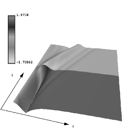
We are now in a position to numerically evolve perturbations about the sphaleron. Figure 5 illustrates the behavior of the $\chi$ field for an initial configuration given by (V) with $c_{4,m=1}=0.00247$ and all other $c$-parameters zero. This is in fact the configuration from which we have chosen to seed the stochastic sampling procedure which we will describe in Sec. VII. We have found it very convenient and informative to use color to code the phase of the complex fields. Unfortunately the illustrations in these pages cannot be reproduced in color and we have tried to render the variation of the phase with a gray scale. At some point a gauge transformation has been performed in Fig. 5 bringing the asymptotic linear state into the sector of zero winding number (consistent with spatial compactification). The gauge transformation is made manifest by the sudden change of shading of the surface. We have performed this gauge transformation because eventually we want to study the topology change of the time reversed solution (cf. Fig. 6 below), and this is best done in a gauge in which the asymptotic linear state has zero winding number. Moreover, the gauge transformation also serves to give a graphic illustration of the gauge invariance of our procedure, which is made manifest by the fact that although the shading (or color) of the surface changes, there is no discontinuity in the surface itself.

From Fig. 5 it is clear that the energy, which is concentrated in the neighborhood of $r=0$, disperses and gives rise to a pattern of outgoing waves. The waves soon become linear and possess a definite particle number, in this case of order $53$ physical particles (using units appropriate to the standard model, which we will refer to as physical units).

The physical process of interest is then the time reversed solution which starts in the linear regime with known particle number, proceeds through the non-linear sphaleron perturbation (V) at intermediate times and finally linearizes once again at late times. Because of time invariance of the equations of motion, this process can be obtained by first evolving the perturbation (V) until the linear regime is reached, and then reversing the momenta and evolving that configuration forward in time. The resulting solution retraces the evolution of the sphaleron decay, and then proceeds over the barrier into another topological sector. Since our numerical strategy for obtaining asymptotically linear topology changing solutions relies upon first evolving the sphaleron perturbation, we shall refer to (V) as the “initial” state, while the asymptotic linear states of the physical process will be called the “in” and “out” states.

FIG. 6.: Topology changing transition: behavior of the $\chi$ field obtained from Fig. 5 by the time reversal procedure described in the text. The various shades of gray code the phase of the complex field. The field starts as an excitation about the trivial vacuum, passes over the sphaleron and then emerges as an excitation about the vacuum of unit winding. Note the persistent strip of $2\pi$ phase change near $r=0$ after the wave bounces off the origin. For a full color figure see http://cthulu.bu.edu/$\scriptstyle\sim$bobs/bviolate.html.

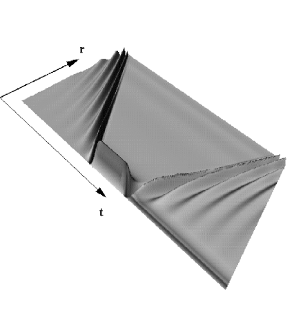
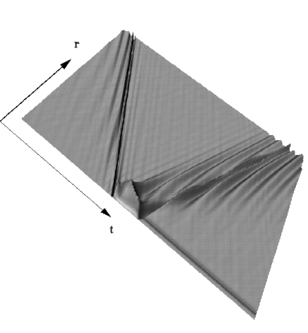
Figure 6 represents a physical process obtained from Fig. 5 in the above manner, and it illustrates the evolution of the $\chi$ field for a topology changing solution. The “initial” state in Fig. 6, determined from (V) by the coefficients $c_{n}$, corresponds to the time-slice half way through the depicted evolution. We have reverted to a gauge in which the boundary conditions are $\chi_{N}=-i$ and $\phi_{N}=1$, consistent with spatial compactification, and in which the in-state has no winding and the out-state has unit winding number. This process represents an imploding spherical energy shell that converges on the origin, where a change of topology takes place. The topology change is indicated by the strip of rapidly varying tonality which persists in the neighborhood of the origin and codes the variation of the $2\pi$ phase change of $\chi$. With color, this strip would appear as a vivid rainbow, left over as a marker of the change of topology of the evolving fields.

It is important to keep in mind that an arbitrary configuration (V) does not necessarily produce a topology changing solution, in the sense that at late times the out-state might evolve back into the original topological sector. With our parameterization (V), however, we have found that the system does in fact typically change topology. Nonetheless, using the time reversed procedure above we can always verify whether the in- and out-states have the same topology, and if so the initial configuration that produced them can be rejected (or equivalently, and more efficiently, we can evolve the initial configuration (V) both forward and backward in time and compare the asymptotic states obtained in this way).

We now have a procedure for constructing solutions which, in the course of their evolution, undergo changes of topology. By varying the values of the parameters $c_{n}$ we will be able to study the properties of such field evolution and, in particular, explore the domain of permissible values for $\epsilon$ and $\nu$. Before we can implement this procedure, however, we must devise a way to calculate the particle number in the asymptotic linear regime. In the next section we describe how this can be done.

VI Normal Modes

Given an initial configuration parameterized by the coefficients $c_{n}$, we evolve the system until the linear regime is reached, where the fields undergo small oscillations about a vacuum configuration. The normal mode amplitudes $a_{n}$ may then be extracted and the particle number computed using (6). We turn now to the problem of identifying the normal modes.

Since we have put the field theoretic system of interest on a spatial lattice, to be entirely consistent we should also solve the normal modes problem on the lattice. The discrete problem, however, cannot be solved analytically and one must resort to numerical methods. On the other hand, the normal modes of the continuum system, even restricted to a box of finite size $L=N\Delta r$, can be found analytically. We have solved the problem both numerically on the lattice and analytically in the continuum limit. The lattice we consider ($N=2239$ with $\Delta r=0.04$) is big enough that there is excellent numerical agreement between the normal modes found by the two methods (the difference between the normalized modes never exceeds $10^{-6}$), so we will present here only the continuum solution.

Following Ref. [16], we work in terms of gauge invariant variables. We write the fields $\chi$ and $\phi$ in polar form,

$$\chi = -i\rho\,e^{i\theta}$$ (140)

$$\phi = \sigma\,e^{i\eta}\ .$$ (141)

The variables $\rho$ and $\sigma$ are gauge invariant. We can also define the gauge invariant angle

$$\xi=\theta-2\eta.$$ (142)

Finally, in 1+1 dimensions we can write

$$r^{2}f_{\mu\nu}=-2\epsilon_{\mu\nu}\psi$$ (143)

where $\epsilon_{01}=+1$ and $\mu$, $\nu$ run over $0$ and $1$. The variable $\psi$ is gauge invariant. Rather than working with the six gauge-variant degrees of freedom $\chi$, $\phi$ and $a_{\mu}$ we use the four gauge invariant variables $\rho$, $\sigma$, $\psi$ and $\xi$. These variables satisfy the equations [16] $$\partial_{\mu}\partial^{\mu}\rho-\frac{\rho\,(\frac{1}{4}r^{2}\sigma^{2}\partial_{\mu}\xi+\epsilon_{\mu\nu}\partial^{\nu}\psi)^{2}}{(\rho^{2}+\frac{1}{4}r^{2}\sigma^{2})^{2}}+\frac{1}{r^{2}}(\rho^{2}-1)\rho+\frac{1}{2}\rho\,\sigma^{2}-\frac{1}{2}\,\sigma^{2}\cos\xi=0$$ (145) $$\partial_{\mu}r^{2}\partial^{\mu}\sigma-\frac{\frac{1}{4}r^{2}\sigma\,(\rho^{2}\partial_{\mu}\xi-\epsilon_{\mu\nu}\partial^{\nu}\psi)^{2}}{(\rho^{2}+\frac{1}{4}r^{2}\sigma^{2})^{2}}+\frac{1}{2}(\rho^{2}+1)\sigma+2\lambda\,r^{2}\left(\sigma^{2}-1\right)\sigma-\rho\sigma\cos\xi=0$$ (146) $$\partial^{\mu}\left\{\frac{\partial_{\mu}\psi-\rho^{2}\epsilon_{\mu\nu}\partial^{\nu}\xi}{\rho^{2}+\frac{1}{4}r^{2}\sigma^{2}}\right\}+\frac{2}{r^{2}}\,\psi=0$$ (147) $$\partial^{\mu}\left\{\frac{\rho^{2}(\frac{1}{4}r^{2}\sigma^{2}\partial_{\mu}\xi+\epsilon_{\mu\nu}\partial^{\nu}\psi)}{\rho^{2}+\frac{1}{4}r^{2}\sigma^{2}}\right\}+\frac{1}{2}\rho\sigma^{2}\sin\xi=0\ ,$$ (148) where the indices run over $0$ and $1$ and are raised and lowered with the metric $\eta_{\mu\nu}={\rm diag}(1,-1)$, so that $\partial_{\mu}\partial^{\mu}=\partial_{t}^{2}-\partial_{r}^{2}$. The energy takes the form

$$\epsilon=4\pi \int_{0}^{\infty}dr\bigg{\{}~{}(\partial_{t}\rho)^{2}+(\partial_{r}\rho)^{2}+r^{2}(\partial_{t}\sigma)^{2}+r^{2}(\partial_{r}\sigma)^{2}+$$ (151)

$$\frac{\frac{1}{4}r^{2}\sigma^{2}\rho^{2}}{\rho^{2}+\frac{1}{4}r^{2}\sigma^{2}}\left[(\partial_{t}\xi)^{2}+(\partial_{r}\xi)^{2}\right]+\frac{1}{\rho^{2}+\frac{1}{4}r^{2}\sigma^{2}}\left[(\partial_{t}\psi)^{2}+(\partial_{r}\psi)^{2}\right]+$$

$$\frac{2\psi^{2}}{r^{2}}+\frac{1}{2r^{2}}(\rho^{2}-1)^{2}+\frac{1}{2}(\rho^{2}+1)\sigma^{2}-\rho\sigma^{2}\cos\xi+\lambda\,r^{2}\left(\sigma^{2}-1\right)^{2}~{}\bigg{\}}\ ,$$

and we see that the vacuum is given by $\rho_{\rm vac}=1$, $\sigma_{\rm vac}=1$, $\psi_{\rm vac}=0$ and $\xi_{\rm vac}=0$.

We wish to consider small fluctuations about the vacuum. It is convenient to define shifted fields $y$ and $h$ by

$$\rho(r,t) = 1+y(r,t)$$ (153)

$$\sigma(r,t) = 1+\frac{h(r,t)}{r}\ .$$ (154)

Then to linear order in $h$, $y$, $\psi$ and $\xi$, (VI) becomes

$$\Biggl{(}\partial_{\mu}\partial^{\mu}+4\lambda\Biggr{)}\,h = 0$$ (156)

$$\Biggl{(}\partial_{\mu}\partial^{\mu}+\frac{1}{2}+\frac{2}{r^{2}}\Biggr{)}\,y = 0$$ (157)

$$\partial^{\mu}\left\{\frac{\partial_{\mu}\psi-\epsilon_{\mu\nu}\partial^{\nu}\xi}{1+\frac{1}{4}r^{2}}\right\}+\frac{2}{r^{2}}\,\psi = 0$$ (158)

$$\partial^{\mu}\left\{\frac{\frac{1}{4}r^{2}\partial_{\mu}\xi+\epsilon_{\mu\nu}\partial^{\nu}\psi}{1+\frac{1}{4}r^{2}}\right\}+\frac{1}{2}\xi = 0\ .$$ (159)

Equation (156) corresponds to a pure Higgs field excitation characterized by mass $m_{H}=2\sqrt{\lambda}$, while (157)-(159) are the three gauge modes of mass $m_{W}=1/\sqrt{2}$. To implement the boundary conditions (III), we take the gauge invariant fields $h$, $y$, $\psi$ and $\xi$ to vanish at $r=0$. At $r=L$ we take $h$, $y$ and $\xi$ to vanish (consistent with $\chi$ and $\phi$ taking their vacuum values there). The $r=L$ boundary condition on $\psi$ is that $\partial_{r}\psi$ is zero ($\psi$ can not vanish at large $r$ since it is proportional to the time derivative of the gauge field). We wish to solve (VI) subject to these boundary conditions, and then extract the corresponding amplitudes.

Let us examine the four types of modes in turn. They can all be expressed in terms of the spherical Bessel functions (V). Equation (156) produces an eigenmode whose non-vanishing components are of the form $h_{n}(r,t)=h_{n}(r)\cos\omega_{1n}t$, with

$$h_{n}(r)=\lambda_{1n}r\,j_{0}(\lambda_{1n}r)\,N_{1n}\ ,$$ (160)

where $\omega_{1n}=(4\lambda+\lambda_{1n}^{2})^{1/2}$ and $\lambda_{1n}=n\pi/L$ for $n=1,2,\cdots$. The parameters $\lambda_{1n}$ have been chosen so that $h_{n}(L,t)=0$, and the normalization constants $N_{1n}$ are taken to be

$$N_{1n}=\left[\,\frac{2}{L}\,\right]^{1/2}$$ (161)

so that the $h_{n}(r)$ are orthonormal over the interval $[0,L]$. To extract these modes from a given solution we expand the Higgs excitation as

$$h(r,t) = \sum_{n}A_{n}\,h_{n}(r)\cos\omega_{1n}t$$ (162)

with

$$A_{n}=\left\{\left[\int_{0}^{L}dr\,h(r,t)h_{n}(r)\right]^{2}+\frac{1}{\omega_{1n}^{2}}\left[\int_{0}^{L}dr\,\dot{h}(r,t)h_{n}(r)\right]^{2}\right\}^{1/2}\ ,$$ (163)

where the dot denotes the time derivative. To find the associated amplitudes, we consider the energy of a pure $h$-excitation. Using (151), and the boundary conditions on $h$, the quadratic energy is

$$H_{h}=\int_{0}^{L}dr\,\left\{(\partial_{t}h)^{2}+(\partial_{r}h)^{2}+4\lambda h^{2}\right\}\ .$$ (164)

Integrating the second term by parts and using the equation of motion (156) we find

$$H_{h} = 4\pi\int_{0}^{L}dr\,\left\{(\partial_{t}h)^{2}-h\,\partial_{t}^{2}h\right\}$$ (166)

$$= 4\pi\sum_{n}A_{n}^{2}\,\omega_{1n}^{2}\ .$$ (167)

Hence, the modulus squared of the amplitudes for this first mode are

$$|a_{1n}|^{2}=4\pi\,A_{n}^{2}\,\omega_{1n}\ ,$$ (168)

where $\omega_{1n}=[4\lambda+(x_{1n}/L)^{2}]^{1/2}$, $x_{1n}=n\pi$ with $n=1,2,\cdots$ and the $A_{n}$ are given by (163).

Equation (157) produces an eigenmode whose non-vanishing components are of the form $y_{n}(r,t)=y_{n}(r)\cos\omega_{2n}t$, with

$$y_{n}(r)=\lambda_{2n}r\,j_{1}(\lambda_{2n}r)\,N_{2n}\ ,$$ (169)

where $\omega_{2n}=(1/2+\lambda_{2n}^{2})^{1/2}$ and $\lambda_{2n}\equiv x_{2n}/L$, with $x_{2n}$ being the positive solutions to $\tan x_{2n}=x_{2n}$ (with this set of modes and those that follow, we will label the normal modes starting from $n=1)$. The parameters $\lambda_{2n}$ have been chosen so that $y_{n}(L,t)=0$, and the normalization constants $N_{2n}$ are taken to be

$$N_{2n}=\left[\,\frac{2}{L\sin^{2}x_{2n}}\,\right]^{1/2}$$ (170)

so that the $y_{n}(r)$ are orthonormal over $[0,L]$. To extract the amplitudes from a given solution we first expand the $y$-excitation as

$$y(r,t) = \sum_{n}B_{n}\,y_{n}(r)\cos\omega_{2n}t$$ (171)

with

$$B_{n}=\left\{\left[\int_{0}^{L}dr\,y(r,t)y_{n}(r)\right]^{2}+\frac{1}{\omega_{2n}^{2}}\left[\int_{0}^{L}dr\,\dot{y}(r,t)y_{n}(r)\right]^{2}\right\}^{1/2}\ .$$ (172)

Using (151), the quadratic energy of a pure $y$-excitation is

$$H_{y}=\int_{0}^{L}dr\,\left\{(\partial_{t}y)^{2}+(\partial_{r}y)^{2}+\frac{y^{2}}{2}+\frac{2y^{2}}{r^{2}}\right\}\ .$$ (173)

Integrating the second term by parts and using the equation of motion (157) we find

$$H_{y} = 4\pi\int_{0}^{L}dr\,\left\{(\partial_{t}y)^{2}-y\,\partial_{t}^{2}y\right\}$$ (175)

$$= 4\pi\sum_{n}B_{n}^{2}\,\omega_{2n}^{2}$$ (176)

Hence, the modulus squared of the amplitudes for the second mode are

$$|a_{2n}|^{2}=4\pi\,B_{n}^{2}\,\omega_{2n}\,$$ (177)

where $\omega_{2n}=[1/2+(x_{2n}/L)^{2}]^{1/2}$, with $x_{2n}$ being the positive solutions of $\tan x_{2n}=x_{2n}$, and where the $B_{n}$ are given by (172).

The remaining two modes are more involved since (158) and (159) are two coupled equations for $\psi$ and $\xi$. To disentangle these modes, we first rewrite these equations as

$$\partial_{t}^{2}\psi-\partial_{r}^{2}\psi+\frac{\psi}{2}+\frac{2\psi}{r^{2}}+\frac{2r}{4+r^{2}}\left[\partial_{r}\psi+\partial_{t}\xi\right] = 0$$ (179)

$$\partial_{t}^{2}\xi-\partial_{r}^{2}\xi+\frac{\xi}{2}+\frac{2\xi}{r^{2}}-\frac{8}{r(4+r^{2})}\left[\partial_{r}\xi+\partial_{t}\psi\right] = 0\ .$$ (180)

We now define $\zeta=r(\partial_{r}\psi+\partial_{t}\xi)/(4+r^{2})$, so that (VI) may be rewritten as

$$\partial_{t}^{2}\psi-\partial_{r}^{2}\psi+\frac{\psi}{2}+\frac{2\psi}{r^{2}}+2\zeta = 0$$ (182)

$$\partial_{t}^{2}\zeta-\partial_{r}^{2}\zeta+\frac{\zeta}{2}+\frac{2\zeta}{r^{2}} = 0\ .$$ (183)

Equation (182) follows directly from (179) and the definition of $\zeta$, while (183) is derived as follows. First, take a time derivative of (180). This gives a $\partial_{t}^{2}\psi$ term in the square brackets, which may be eliminated using (182) to give

$$\partial_{t}^{2}\dot{\xi}-\partial_{r}^{2}\dot{\xi}+\frac{\dot{\xi}}{2}+\frac{2\dot{\xi}}{r^{2}}-\frac{8}{r(4+r^{2})}\left[\partial_{r}\dot{\xi}+\partial_{r}\psi^{\prime}-2\zeta\right]+\frac{4\psi}{r^{3}}=0\ ,$$ (184)

where the dot and prime denote time and space derivatives respectively. We have written $\partial_{t}^{2}\dot{\xi}$ rather than $\partial_{t}^{3}\xi$, $\partial_{r}\psi^{\prime}$ rather than $\partial_{r}^{2}\psi$, etc. for future convenience. Taking a spatial derivative of (182) gives

$$\partial_{t}^{2}\psi^{\prime}-\partial_{r}^{2}\psi^{\prime}+\frac{\psi^{\prime}}{2}+\frac{2\psi^{\prime}}{r^{2}}-\frac{4\psi}{r^{3}}+2\zeta^{\prime} = 0\ .$$ (185)

Adding (184) and (185), and using $\dot{\xi}+\psi^{\prime}=(4+r^{2})\zeta/r$ gives (183).

These normal modes fall into two classes, one in which $\zeta=0$ and another in which $\zeta$ is non-vanishing. In the former case, (182) may be solved for $\psi$. We may then use $\partial_{t}\xi+\partial_{r}\psi=0$ to solve for $\xi$. Thus, mode three takes the form $\psi_{3n}(r,t)=\psi_{3n}(r)\sin\omega_{3n}t$ and $\xi_{3n}(r,t)=\xi_{3n}(r)\cos\omega_{3n}t$, and after some algebra we find

$$\psi_{3n}(r) = \lambda_{3n}r\,j_{1}(\lambda_{3n}r)\,N_{3n}$$ (187)

$$\xi_{3n}(r) = \frac{\lambda_{3n}}{\omega_{3n}}\left[2j_{1}(\lambda_{3n}r)-\lambda_{3n}r\,j_{2}(\lambda_{3n}r)\right]\,N_{3n}\ ,$$ (188)

where $\omega_{3n}=(1/2+\lambda_{3n}^{2})^{1/2}$ and $\lambda_{3n}\equiv x_{3n}/L$, with $x_{3n}$ being the positive solutions to $\tan x_{3n}=x_{3n}/(1-x_{3n}^{2})$. The parameters $\lambda_{3n}$ have been chosen so that $\xi_{3n}(L,t)=0$ (since $\zeta$ vanishes, this automatically ensures that $\partial_{r}\psi_{3n}(L,t)=0$). The normalization constants $N_{3n}$ will be chosen below to ensure a convenient orthonormality relation for the $\psi_{3n}(r)$ and $\xi_{3n}(r)$.

We turn now to the other class of modes in which $\zeta$ is non-vanishing. We can first solve (183) for $\zeta$, and then solve (182) for $\psi$ treating $\zeta$ as a source. Then, using the definition of $\zeta$, we can solve for $\xi$. Again, writing $\psi_{4n}(r,t)=\psi_{4n}(r)\sin\omega_{4n}t$ and $\xi_{4n}(r,t)=\xi_{4n}(r)\cos\omega_{4n}t$, we find

$$\psi_{4n}(r) = \frac{r}{\lambda_{4n}^{2}}\left[2j_{1}(\lambda_{4n}r)-\lambda_{4n}r\,j_{0}(\lambda_{4n}r)\right]\,N_{4n}$$ (190)

$$\xi_{4n}(r) = \frac{1}{\lambda_{4n}^{2}\omega_{4n}}\left[-2\lambda_{4n}r\,j_{0}(\lambda_{4n}r)+4(1-\lambda_{4n}^{2})j_{1}(\lambda_{4n}r)-2\lambda_{4n}r\,j_{2}(\lambda_{4n}r)\right]\,N_{4n}\,$$ (191)

where $\omega_{4n}=(1/2+\lambda_{4n}^{2})^{1/2}$ and $\lambda_{4n}\equiv x_{4n}/L$, with $x_{4n}$ being the positive solutions to $\tan x_{4n}=x_{4n}$. The parameters $\lambda_{4n}$ have been chosen so that $\xi_{4n}(L,t)=0$ and $\partial_{r}\psi_{4n}(L,t)=0$, and the normalization constants $N_{4n}$ will be chosen below.

We expand a $\psi$-$\xi$ excitation as

$$\psi(r,t) = \sum_{j=3,4}\sum_{n}C_{jn}\,\psi_{jn}(r)\sin\omega_{jn}t$$ (193)

$$\xi(r,t) = \sum_{j=3,4}\sum_{n}C_{jn}\,\xi_{jn}(r)\cos\omega_{jn}t\ .$$ (194)

Choosing the normalization constants

$$N_{3n} = \left[\,\frac{(2-x_{3n}^{2})\sin^{2}x_{3n}}{2Lx^{4}_{3n}}+\frac{x_{3n}^{4}-x_{3n}^{2}-2}{2Lx_{3n}^{2}}\,\right]^{-1/2}$$ (196)

$$N_{4n} = \left[\,\frac{L^{3}(2x_{4n}^{6}+L^{2})\sin^{2}x_{4n}}{x_{4n}^{8}}+\frac{L^{5}(x_{4n}^{2}-1)}{x_{4n}^{6}}\,\right]^{-1/2}\ ,$$ (197)

the modes satisfy the orthonormality relations

$$\int_{0}^{L}dr\,\Bigg{\{}\,\frac{r^{2}}{4+r^{2}}\,\omega_{jn}\xi_{jn}(r)\,\omega_{km}\xi_{km}(r)+\frac{4}{4+r^{2}} \,\partial_{r}\psi_{jn}(r)\,\partial_{r}\psi_{km}(r)$$ (200)

$$+\frac{2}{r^{2}}\,\psi_{jn}(r)\psi_{km}(r)\Bigg{\}}=\delta_{nm}\delta_{jk}$$

$$\int_{0}^{L}dr\,\Bigg{\{}\,\frac{4}{4+r^{2}}\,\omega_{jn}\psi_{jn}(r)\,\omega_{km}\psi_{km}(r)+\frac{r^{2}}{4+r^{2}} \,\partial_{r}\xi_{jn}(r)\,\partial_{r}\xi_{km}(r)$$ (202)

$$+\frac{1}{2}\,\xi_{jn}(r)\xi_{km}(r)\Bigg{\}}\hskip 7.22743pt=\delta_{nm}\delta_{jk}\ .$$

Using (VI) in (VI), the overlap coefficients $C_{jn}$ become

$$C_{jn}= \Bigg{\{}\Bigg{[}\int_{0}^{L}dr\Bigg{(}-\omega_{jn}\frac{r^{2}}{4+r^{2}}\,\partial_{t}\xi(r,t)\,\xi_{jn}(r)$$ (206)

$$+\frac{4}{4+r^{2}}\partial_{r}\psi(r,t)\,\partial_{r}\psi_{jn}(r)+\frac{2}{r^{2}}\,\psi(r,t)\psi_{jn}(r)\Bigg{)}\Bigg{]}^{2}$$

$$+\Bigg{[}\int_{0}^{L}dr\Bigg{(}\omega_{jn}\frac{4}{4+r^{2}}\,\partial_{t}\psi(r,t)\,\psi_{jn}(r)$$

$$+\frac{r^{2}}{4+r^{2}}\,\partial_{r}\xi(r,t)\,\partial_{r}\xi_{jn}(r)+\frac{1}{2}\,\xi(r,t)\xi_{jn}(r)\Bigg{)}\Bigg{]}^{2}\Bigg{\}}^{1/2}\ .$$

To extract the amplitudes, consider a pure $\psi$-$\xi$ excitation. Using (151), the quadratic energy is given by

$$H_{\xi\psi} = 4\pi\int_{0}^{L}dr\,\left\{\frac{r^{2}}{4+r^{2}}\left[\dot{\xi}^{2}+\xi^{\prime 2}\right]+\frac{4}{4+r^{2}}\left[\dot{\psi}^{2}+\psi^{\prime 2}\right]+\frac{2\psi^{2}}{r^{2}}+\frac{\xi^{2}}{2}\right\}$$ (208)

$$= 4\pi\sum_{j=3,4}\sum_{n}C_{jn}^{2}\ ,$$ (209)

hence

$$|a_{jn}|^{2}=4\pi\,\frac{C_{jn}^{2}}{\omega_{jn}}\qquad j=3,4\ .$$ (210)

Even though we have solved the normal modes problem analytically in the continuum, the amplitudes $|a_{jn}|^{2}$ will be extracted using discrete numerical solutions. This is justified by the large size of our lattice: $N=2239$, $\Delta r=0.04$ (with $\lambda=0.1$).

For computational purposes it is important to note that, strictly speaking, completeness sums involve all normal modes, but in a physically meaningful situation they will be saturated well before the normal mode indices reach the maximum value $N$. The highest normal modes indeed correspond to artifacts of the discretization. Thus, to avoid unnecessary computational burdens, we will place a cutoff ${N_{\rm mode}}\sim N/5$ to $N/10$ on the number of normal modes and calculate the Higgs and gauge boson particle numbers as

$$\nu_{\rm higgs} = \sum_{n=1}^{N_{\rm mode}}|a_{1n}|^{2}$$ (212)

$$\nu_{\rm gauge} = \sum_{n=1}^{N_{\rm mode}}\left\{|a_{2n}|^{2}+|a_{3n}|^{2}+|a_{4n}|^{2}\right\}\ .$$ (213)

The total particle number is given by

$$\nu=\nu_{\rm higgs}+\nu_{\rm gauge}\ .$$ (214)

We have verified that our results are insensitive to this cutoff, which means that short wavelength modes comparable to the lattice spacing are not excited in any appreciable manner. One should also note that our procedure for calculating the particle number is obviously gauge invariant (as it should be) since it makes use of an expansion into normal modes of gauge invariant variables.

FIG. 7.: Decay of a small perturbation about the sphaleron: behavior of the particle number in the four normal modes of oscillation of the linearized system as function of time for lattice parameters $N=2239$, $\Delta r=0.04$ and $N_{\rm mode}=200$ with $\lambda=0.1$. The physical particle numbers are obtained by multiplying the asymptotic values in the graph by $4\pi/g^{2}\sim 30$, which gives $N_{\rm higgs}\sim 8$ and $N_{\rm gauge}\sim 45$, for a total physical particle number of $N_{\rm phys}\sim 53$.

In Fig. 7 we display the behavior of the particle number in the four normal modes of oscillation as function of time. The initial state is the small perturbation about the sphaleron in Fig. 5, which gives rise to outgoing spherical waves as the configuration decays. This is the state from which we start the stochastic sampling procedure described in the next section. Since the energy density is distributed over an expanding shell, the system quickly approaches the linear regime. This is apparent from Fig. 7 where, after an initial transition period in which the particle numbers of the four modes are not constant, they settle to values which are reasonably constant in time. We take this as evidence that the system has indeed reached an asymptotic linear regime where one can define a conserved particle number.

There are two additional quantities that are useful in measuring the extent of linearity, namely the spectral energy $\epsilon_{\rm spec}$ and the linearized energy $\epsilon_{\rm lin}$. The spectral energy is defined as the sum over normal mode energies,

$$\epsilon_{\rm spec}=\sum_{n=1}^{N_{\rm mode}}\left\{\omega_{1n}|a_{1n}|^{2}+\omega_{2n}|a_{2n}|^{2}+\omega_{3n}|a_{3n}|^{2}+\omega_{4n}|a_{4n}|^{2}\right\}\ ,$$ (215)

while the linearized energy is defined by integrating the energy density in (151) expanded to second order in a perturbation about the vacuum,

$$\epsilon_{\rm lin} = 4\pi\int_{0}^{\infty}dr\bigg{\{}~{}(\partial_{t}y)^{2}+(\partial_{r}y)^{2}+\frac{2y^{2}}{r^{2}}+\frac{y^{2}}{2}+(\partial_{t}h)^{2}+(\partial_{r}h)^{2}+4\lambda h^{2}+$$ (217)

$$\frac{r^{2}}{4+r^{2}}\left[(\partial_{t}\xi)^{2}+(\partial_{r}\xi)^{2}\right]+\frac{\xi^{2}}{2}+\frac{4}{4+r^{2}}\left[(\partial_{t}\psi)^{2}+(\partial_{r}\psi)^{2}\right]+\frac{2\psi^{2}}{r^{2}}\bigg{\}}\ .$$

Both the spectral and linear energy are gauge invariant since they have been defined using gauge invariant quantities. If the system linearizes, then both $\epsilon_{\rm spec}$ and $\epsilon_{\rm lin}$ should be close to the conserved total energy $\epsilon$, which is given by the integral (151) (or in terms of gauge-variant variables by (III)). The total energy of the configuration in Fig. 7 is given by $\epsilon/4\pi=2.5447$, while the asymptotic spectral and linear energies are given by $\epsilon_{\rm spec}/4\pi=2.5679$ and $\epsilon_{\rm lin}/4\pi=2.5685$, and we see that the system has linearized to within one percent. (We also see that the sum over the energies of individual modes, although cut off at $N_{\rm mode}$, essentially accounts for all the linearized energy.)

FIG. 8.: Mode distribution for the asymptotic state of Figs. 5 and 7. This distribution is gauge invariant, and shows that all the particle are rather soft and comparable in energy.

We can also investigate the mode distribution by examining the amplitudes $|a_{jn}|^{2}$ as a function of mode number $n$. As the system linearizes and the particle number becomes well defined, the mode distribution also becomes constant in time. Figure 8 illustrates the distribution of the asymptotic linear state of Figs. 5 and 7. Note that the population of the system is heavily weighted towards low lying modes. The mode cutoff used in calculating the particle number was $N_{\rm mode}=200$, and we see that modes greater than about $n=150$ are not populated to any appreciable extent. The mode distributions are heavily peaked near $n_{\rm pk}\sim 50$, which corresponds to a frequency of $\omega_{\rm pk}\sim n_{\rm pk}\pi/L\sim 0.1$. The perturbation about the sphaleron of Figs. 5 and 7 decays into about $50$ rather soft particles (in physical units), each one of comparable energy. Finally, we point out that the mode distribution is gauge invariant as well.

VII Stochastic Sampling of Initial Configurations

As we have discussed, our goal is to find the region in the $\epsilon$-$\nu$ plane spanned by all topology changing classical solutions. More specifically, we would like to find the lower boundary of this region. The tools we have at our disposal allow us to vary the coefficients $c_{n}$ of (V), which defines the system as it passes over the sphaleron barrier, and to calculate the corresponding energy $\epsilon$ and incoming particle number $\nu$. From the computational point of view, $\epsilon$ and $\nu$ can be considered as known functions (albeit laboriously obtained) of the variables $c_{n}$. We would then like to find

$$\nu_{\rm lower}(\epsilon)={\rm Min}_{\{c{\scriptscriptstyle n},\,{\rm fixed}\;\epsilon\}}\;\nu\ .$$ (218)

The particle number $\nu$ may have several local minima since it is a highly non-linear function of the variables $c_{n}$, and a straightforward constrained minimization procedure, such as a conjugate gradient technique, could fail to reveal the absolute minimum of $\nu$ at a given $\epsilon$. We therefore decided to solve the problem using stochastic sampling. Stochastic sampling methods, driven by suitable weight functions and in combination with annealing techniques, have indeed proven very effective in exploring the overall structure of complicated surfaces and in approximating their global minima.

Our procedure consists in generating “configurations” of the system weighted by a function

$$W=\exp(-F)\ ,$$ (219)

with

$$F=\beta\,\epsilon\,-\mu\,\nu\ .$$ (220)

By “configuration” simply we mean the collection of variables $c_{n}$, which determine the whole evolution of the system. Since $\epsilon$ and $\nu$ are functions of $c_{n}$, the weight given by (219) and (220) is also a function of $c_{n}$ and defines a probability distribution

$$dP=Z^{-1}\,\prod_{n}dc_{n}\,W(c_{n})\ .$$ (221)

We will generate topology changing configurations distributed according to (221). Clearly, by taking large values for the parameters $\beta$ and $\mu$ we will drive the distribution strongly towards the lower boundary in the space of all topology changing solutions. By using different ratios $\mu/\beta$ we will be able to drive the distribution in different direction and thus follow the lower envelope of the region, while temporarily lowering the values of $\mu$ and/or $\beta$ will allow us to anneal the distribution. We will typically take $\beta$ between $50$ and $1,000$ while $\mu$ will range between $1,000$ and $20,000$.

To generate the desired distribution we have used a Metropolis Monte Carlo algorithm. Starting from a definite configuration $c_{n}$, we randomly select one of the variables $c_{i}$ and perform a variation $c_{i}\to c_{i}^{\prime}=c_{i}+\Delta c_{i}$ (in our computation, the $\Delta c_{i}$ are Gaussian distributed with a mean of 0.0008.) The system is evolved backward and forward in time and we calculate the energy, in-state particle number and change of winding number. If the winding number does not change, we proceed to vary another of the variables $c_{n}$. If the topology changes, we evaluate $\Delta F=\beta\Delta\epsilon+\mu\Delta\nu$ and the new value $c_{i}^{\prime}$ is accepted with conditional probability $p={\rm Min}[1,\exp(-\Delta F)]$. Specifically, we generate a pseudorandom number $r$ uniformly distributed between $0$ and $1$, and if $r\leq\exp(-\Delta F)$ the change is accepted and the new value $c_{i}^{\prime}$ replaces the old one. Otherwise, if $r>\exp(-\Delta F)$ the old value is kept and we select another of the variables $c_{n}$ for a possible upgrade. (We should note here that when the winding number changes, even if the trial value $c_{i}^{\prime}$ is rejected, we still record its value and the corresponding values of $\epsilon$ and $\nu$, since they do correspond to a possible topology changing evolution.)

It must be emphasized that although our algorithm generates a distribution of topology changing solutions of the equations of motion, this distribution represents only a computational device and carries no special physical significance. Indeed, the probability measure (221) is based on the arbitrary choice of variables $c_{n}$ and no Jacobian factor of any kind has been introduced. It would be possible to define a measure which represents a physically meaningful distribution, and our notation $\beta$ and $\mu$ for the weights of $\epsilon$ and $\nu$ has been inspired by the analogy with a grand canonical ensemble. But still, in the present context, there is no reason for defining any particular physically meaningful measure and no justification for the attached computational costs.

FIG. 9.: Monte Carlo results with lattice parameters of $N=2239$, $\Delta r=0.04$ (giving L=89.56), $N_{\rm mode}=200$ and $N_{\rm sph}=50$, and with a Higgs self-coupling of $\lambda=0.1$. The solid line marks the sphaleron energy $\epsilon_{\rm sph}=4\pi(2.5426)$, below which no topology changing process can lie. The diamond represents the configuration from which we seeded our Monte Carlo search. To obtain quantities in physical units, multiply the numbers along the axes by $4\pi/g^{2}\sim 30$. The energy axis extends from about $10{~{}\rm TeV}$ to $15{~{}\rm TeV}$, while the particle number axis ranges from about $30$ particles to $60$.

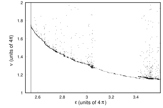
Figure 9 illustrates the results of our Monte Carlo investigation. It represents about 300 hours of CPU time on a 16 node partition of a CM-5. We generated approximately 30,000 configurations of which approximately 3,000 representatives are plotted in the figure. We have chosen lattice parameters $N=2239$ and $\Delta r=0.04$, for a lattice of size $L=89.56$. We have used a cutoff $N_{\rm mode}=200$ on the sums over the modes, and the dimension of the initial configuration space over which we have sampled is determined by $N_{\rm sph}=50$. We have taken the Higgs self-coupling to be $\lambda=0.1$, which in lattice units corresponds to a mass of about $m_{H}=(40\Delta r)^{-1}$, or a physical mass of $m_{H}=110{~{}\rm GeV}$. As one can see, our lattice is sufficiently dense that there are many lattice sites within a single Higgs Compton wavelength.

It is apparent from Fig. 9 that our search procedure is effective in reducing the particle number and in exploring the lower boundary of the space of topology changing classical solutions. The complex nature of this space (or at least of our search procedure) is also apparent from the figure, in that one can clearly observe two breaks in the outline of the lower boundary at $\epsilon/4\pi\sim 3$ and $\epsilon/4\pi\sim 3.4$. The reason for the discontinuity is that in a first extended search we did not verify that every individual solution changed topology (performing this check is costly in computer time), trusting that topology change would be the typical outcome of an evolution which passes over the sphaleron barrier. A subsequent analysis revealed however that for a whole subset of our configurations, comprised between $\epsilon/4\pi\sim 3$ and $\epsilon/4\pi\sim 3.4$, the topology did not change: the system went over the sphaleron barrier a second time in the reversed direction and returned to the original topological sector. We discarded all these configurations and verified that the topology changed in all the remaining ones. We then implemented the check for topology change at every Monte Carlo step and restarted our sampling procedure by annealing a topology changing configuration obtained for $\epsilon/4\pi\sim 3$. This second search produced the set of configurations which stand out at slightly lower $\nu$ between $\epsilon/4\pi\sim 3$ and $\epsilon/4\pi\sim 3.4$.

FIG. 10.: Topology changing transition obtained after many Monte Carlo iterations: behavior of the $\chi$ field. For a full color figure see http://cthulu.bu.edu/$\scriptstyle\sim$bobs/bviolate.html.

Our search procedure not only leads to classical solutions with lower particle number, but is effective in selecting configurations with special properties in the in-state (these two features of course go hand in hand). In Fig. 10 we illustrate the entire evolution for one of the topology changing processes with low particle number, corresponding to one of the points at the bottom-right corner of the plot in Fig. 9. Figure 10 should be contrasted with Fig. 6 in which the evolution of our Monte Carlo seed configuration is illustrated. The change is dramatic. The in- and out-states in Fig. 6 look rather symmetric, up to the topology change of the out-state concentrated about the origin. The particle numbers of the in- and out-states are about the same and of order $50$ in physical units ($\nu_{i}/4\pi=1.747$ and $\nu_{o}/4\pi=1.750$, respectively). Figure 9 shows that after many Monte Carlo iterations we have managed to filter initial configurations $c_{n}$ so that the in-state particle numbers are about $40\%$ lower ($\nu_{i}/4\pi\sim 1.10$), and from Fig. 10 it is apparent that the in-states are now much different from the out-states. The former are narrow with the spectrum shifted towards shorter wavelengths, while the outgoing states still display the broad long-range waves seen at both ends of the evolution in Fig. 6. Indeed, the particle number in the out-state remains high.

FIG. 11.: Behavior of the in-state particle number in the four normal modes. The initial state was obtained after many Monte Carlo iterations, and soon linearizes. Note, however, that mode 3 remains about 10% non-linear.

More details of the configurations selected by our sampling procedure are revealed by Figs. 11 and 12. Figure 11 illustrates the behavior of the particle numbers associated with the four normal modes for the initial configuration $c_{n}$ used to generate Fig. 10. The asymptotic particle numbers in Fig. 11 are associated with the in-state of the physically relevant time reversed solution of Fig. 10. Figure 12 illustrates the mode distribution of this in-state. These figures should be contrasted with Figs. 7 and 8 which display the same quantities at the beginning of our search. The change is again very impressive. In particular, it is clear that the stochastic sampling procedure has selected classical solutions where the mode distribution in the in-states is shifted towards higher frequencies and shorter wavelengths. Of course, this is necessary for a reduction of the ratio $\nu/\epsilon$.

FIG. 12.: Mode distribution of the asymptotic in-state of Fig. 11.

Although our results show a marked decrease in the particle number of the incoming state, nowhere in the energy range we have explored does $\nu$ drop below $4\pi$, or in physical units $N_{\rm phys}{\ \lower-1.2pt\vbox{\hbox{\hbox to0.0pt{$>$\hss}\lower 5.0pt\vbox{\hbox{$\sim$}}}}\ }30$ for $E{\ \lower-1.2pt\vbox{\hbox{\hbox to0.0pt{$<$\hss}\lower 5.0pt\vbox{\hbox{$\sim$}}}}\ }15{~{}\rm TeV}$. This is a far cry from the value $N_{\rm phys}=2$ which would be needed to argue that baryon number violation can occur in a high energy collisions. From this point of view our present results are limited and should be pushed to much higher values of $\epsilon$. In the next section we will make some comments about our future plans to explore higher energies and discuss other investigations which can shed further light on the properties of the system. As of now the computational resources at our disposal, together with the rather ambitious number of points we have used for our numerical study, have not permitted us to go beyond the energy range we have explored. We believe that our results, as well as the formalism we have established, are nevertheless interesting enough to warrant publication. In some respect, the choice of a number of points as large as our current $N=2239$ has been an error of strategy. In a preliminary investigation, described in [17], we had used $N=256$. The number of points in the lattice determines of course the ultraviolet cutoff and this in turn implies a minimum value for the ratio $\nu/\epsilon$. This quantity is indeed minimized by placing all the weight in the highest mode $N_{\rm mode}$, giving $(\nu/\epsilon)_{\rm min}=1/\omega_{\rm mode}\sim L/N_{\rm mode}\pi$. With $N=256$ points we saw the onset of this constraint, and we decided to chose a lattice size that would push the lower limit on $\nu/\epsilon$ to a much smaller value closer to the physically relevant domain. With the parameters of our present calculation, the minimum would occur at $(\nu/\epsilon)_{\rm min}\sim 0.15$. However, the increased computational burden, together with the fact that the stochastic sampling moved in the $\epsilon$-$\nu$ plane at a much slower rate than we had anticipated, prevented us from saturating this lower bound.

It is still interesting to extrapolate our results to obtain information about the possible behavior of the boundary in the $\epsilon$-$\nu$ plane of topology changing solutions. For this purpose we binned all our data into subintervals of width $\Delta\epsilon=0.005$. Within every bin we selected the point with lowest $\nu$. We then fitted these points to the hyperbola

$$(\nu-\alpha\epsilon-c_{1})(\nu-\nu_{\infty})=c_{2}\ ,$$ (222)

where $\alpha$ and $\nu_{\infty}$ are the free parameters of the fit. The quantities $c_{1}$ and $c_{2}$ (which are constants with respect to $\nu$ and $\epsilon$ but depend on $\alpha$ and $\nu_{\infty}$) are given by $c_{1}=2\nu_{\rm sph}-\alpha\epsilon_{\rm sph}-\nu_{\infty}$ and $c_{2}=-(\nu_{\rm sph}-\nu_{\infty})^{2}$, where $\epsilon_{\rm sph}=2.5447$ and $\nu_{\rm sph}=1.7478$ are the energy and particle number in the limiting case in which the configuration approaches the sphaleron itself (in practice the $\epsilon$ and $\nu$ of the configuration from which we started the Monte Carlo search).

This fit is motivated by simple physical considerations. We would expect the lower boundary of the region of topology changing transitions to saturate either at $\nu=0$ or at some finite value of $\nu$. The boundary of the domain must go through the sphaleron and should have an infinite slope there. Indeed, since the topology changing classical solutions become complex when $\epsilon$ decreases below $\epsilon_{\rm sph}$, one would expect the boundary curve $\nu=\nu(\epsilon)$ to have a square root singularity at $\epsilon=\epsilon_{\rm sph}$. Finally, although the upper boundary of the region is of little interest to us, it is not unreasonable to parameterize it in terms of a straight line of constant slope. This is the line one would find if the upper bound were obtained by putting all the energy in a single mode of frequency $\omega$ (in which case the slope $\alpha=1/\omega$), or since this is unrealistic, if the the mode distribution could be well approximated in terms of some effective frequency $\omega_{\rm eff}=1/\alpha$. The hyperbola of (222) is the simplest curve with all these properties.

The results of our fits are shown in Figs. 13 and 14. In Fig. 13 all the data points have been used, and the solid line represents the unconstrained fit while the dashed line is obtained by requiring $\nu_{\infty}=0$. Since one can argue that what ought to be fit is the lower boundary of the region, and that insofar as our points display a slight discontinuity and cannot all belong to this boundary, we have repeated the fit removing all the points which lie above the unconstrained fit in Fig. 13. The results of this second fit are reproduced in Fig. 14. For Fig. 13, the unconstrained fit has parameters $\alpha=0.257$ and $\nu_{\infty}=-0.294$ while the constrained fit has $\alpha=0.319$. Figure 14 has the parameters $\alpha=0.238,\nu_{\infty}=-0.530$ and $\alpha=0.341$ respectively for the unconstrained and constrained fits.

FIG. 13.: Hyperbolic fits to full data set. The asymptotic particle number is constrained to vanish for the dashed line, while it remains unconstrained for the solid line.

FIG. 14.: Same as Fig. 13, except the data set was reduced by those point lying above the previous unconstrained fit.

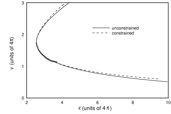
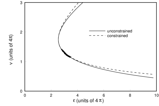
It is interesting to observe that that the unconstrained fits lead to an asymptotic value for $\nu$ smaller than zero, which shows that one cannot read any indication of a lower bound on the particle number in our present data. Our results cover a range of energies which is too small to derive any reliable conclusion about whether and when the particle number could reach the value two. One can nevertheless insert physical units in the results of our fits and see at what energy values the incident particle number would become equal to two. This simple exercise gives energies of $110.37{~{}\rm TeV}$ and $447.20{~{}\rm TeV}$ respectively for the unconstrained and constrained fits of Fig. 13, and energies of $75.06{~{}\rm TeV}$ and $418.61{~{}\rm TeV}$ for the corresponding fits of Fig. 14.

We conclude this section with a few technical remarks. Since our entire procedure is based on the calculation of the particle number after the system has reached the linear regime, we should make sure this quantity is evaluated in a reliable manner. Now, it is clear from the graphs of Figs. 7 and 11 that, while the particle number becomes reasonably constant towards the end of the evolution, it still exhibits oscillations possibly as large as 10%. This might cast doubts on the validity of our stochastic sampling technique, where the steps in initial parameter space induce variations of the particle number as small as $10^{-4}$. The solution we have adopted is to define a “computational particle number” $\nu_{c}$ (which is the quantity represented in Fig. 9). With a lattice of infinite spatial extent, even in presence of an ultraviolet cutoff arising from finite lattice spacing, and barring the existence of conservation laws giving rise to particle phenomena, the system will eventually linearize fully and the true particle number $\nu$ will be well defined and constant to any degree of precision. Since we begin with an initial state localized around the origin, we may conceptually think of this as being defined over an infinite lattice, although in practice we use a lattice of finite extent. Thus, every initial configuration $c_{n}$ conceptually determines a unique particle number $\nu$. This may not be accessible to us, but it exists. We define a quantity $\nu_{c}$ which we can measure as follows: we evolve the system for a definite amount of time $T_{0}$ and then for an additional time $\Delta T$ (in our calculation $T_{0}=60$ and $\Delta T=8$). Over the interval $T_{0},\,T_{0}+\Delta T$ we measure the particle number at times $T_{i}=T_{0}\dots T_{m}$ chosen at random (in our calculation we take $m=10$ and choose $T_{1}$ through $T_{10}$ to be 61.55, 62.51, 63.27, 63.70, 64.77, 65.25, 65.33, 65.71, 66.59, 68.00 respectively), but fixed for the entire calculation. The computational particle number $\nu_{c}$ is defined as the average of the particle numbers measured at $T_{i}$. Again, $\nu_{c}$ is a well defined function of the parameters $c_{n}$, and uniquely determined by this initial configuration. The crucial point is that $\nu_{c}$ tracks $\nu$. The quantities $\nu$ and $\nu_{c}$ may differ by as much as 10%; however, if we reduce $\nu_{c}$ by a certain factor, we can be confident that the true particle number $\nu$ has also been reduced by the same factor, up to a relative error given by the approximation by which $\nu_{c}$ tracks $\nu$. Finally, we should make sure that $\nu_{c}$ is, computationally, a well behaved function of the parameters $c_{n}$, i.e. that the functional relation between the chosen $c_{n}$ and the measured value of $\nu_{c}$ is not spoiled by numerical errors. This we have verified explicitly. On a sample configuration we have stepped every individual parameter $c_{n}$ by values an order of magnitude smaller than the typical steps in our stochastic sampling procedure and have verified that the corresponding changes in $\nu_{c}$ are regular and well accounted for by the first few terms of a Taylor series expansion in $\Delta c_{n}$.

VIII Conclusions

We have developed a computational procedure that allows us to explore the space of classically allowed topology changing transitions leading to baryon number violation. With our method we have been able to trace the lower boundary of the region spanned by topology changing evolution in the energy versus incoming particle number plane, up to energies approximately one and a half times the sphaleron energy and with a reduction of the incoming particle number by approximately 40%. The corresponding solutions display dramatically different features in their incoming state from the solution used to seed the Monte Carlo search (in which there was just barely enough energy to cross the sphaleron barrier), one of the most notable differences being a marked shift of the in-state spectral mode distribution towards higher frequencies and shorter wavelengths. Within the domain we have explored there is no indication of an emergent lower limit on the particle number of the incoming state. Indeed, a hyperbola fit to our data, motivated by the expected physical properties of the boundary of the domain of topology changing evolution, is quite compatible with a zero lower bound on the incoming particle number.

Our results are unfortunately rather limited in the extent of energy and particle number which we have been able to explore. However impressive may be the change in the properties of the solutions spanned by our search, the fact remains that the lowest particle number we have been able to reach is, in physical units, approximately 30. An even more serious shortcoming of our results is that our method can only establish an upper bound on the minimum particle number at any given energy: when our search produces a topology changing solution of given $\epsilon$ and $\nu$, it establishes by construction that the lower boundary of the classically allowed transitions cannot lie above that point, but we cannot rule out that it might lie substantially below and that the stochastic search simply failed to come close to it.

However, the mere fact that the analytically intractable non-linear equations of motion are amenable to a reliable computational solution is, we believe, a very important result, perhaps the most important fact emerging from our analysis. By solution, we mean much more than just the implementation of a numerical integration algorithm of the evolution equations. Our study makes it clear that a whole range of detailed questions about the entire space of solutions can be tackled and solved by computational means.

The results we have established thus far naturally lead to further investigation. By investing more computational resources it will be straightforward to extend the exploration to substantially larger energies. However, one can do more than that. The detailed information obtained about the spectral composition of the incoming states with low particle number suggests that that one may explore the properties of such states directly. For instance, one could try to shift the mode distribution further towards shorter range, while verifying that the ensuing evolution still changes topology. This runs somehow against our original notion that it would be very difficult to start from the selection of the incoming state and still obtain a topology changing solution, but now we are no longer dealing with a blind sampling of incident states. From this point of view we find very inspiring some recent results obtained by Farhi, Goldstone, Lue and Rajagopal who, in a study of collision induced soliton decay, were able to produce the “unwinding” of the soliton and its subsequent decay by directing against it waves which carry a short range twist of the phase of the complex field (we refer to the original work of Ref. [18] for an elucidation of this possibly cryptic sentence). It is interesting that in computer animation which we generated to clarify the properties of the evolution, we have seen analogous twists in the phase of the 2-dimensional field $\chi$ in the asymptotic states. Of course one must be careful in defining effects which pertain to gauge variant quantities, but a careful study of the properties of the asymptotic states may provide important clues for understanding the mechanisms leading to classically allowed transitions with low incoming particle number.

Finally, a complementary approach to the study of classically allowed transitions consists in studying the classically forbidden processes. As we have already mentioned in the Introduction, a very powerful formalism for the study of such processes has been established in Ref. [6] and applied recently in Ref. [19] to the study of collision induced decay of the false vacuum. The method of Ref. [6] requires that one solves analytically continued equations of motion along a suitable contour in the complex time plane and that one imposes boundary conditions based on the normal mode expansion of the fields in the linearized domain. Thus a large part of the formalism we have developed in this paper will carry over to the study of classically forbidden processes, and we plan to make this the subject of a future investigation.

Acknowledgments

This research was supported in part under DOE grant DE-FG02-91ER40676 and NSF grant ASC-940031. We wish to thank V. Rubakov for very interesting conversations which stimulated the investigation described here, A. Cohen, K. Rajagopal and P. Tinyakov for valuable discussions, and T. Vaughan for participating in an early stage of this work.

REFERENCES

- [1] G. ’t Hooft, Phys. Rev. D14 (1976) 3432.
-
[2]
N. Manton, Phys. Rev. D28 (1983) 2019;
F. Klinkhamer and N. Manton, Phys. Rev. D30 (1984) 2212. - [3] A. Ringwald, Nucl. Phys. B330 (1990) 1.
- [4] O. Espinosa, Nucl. Phys. B343 (1990) 310.
- [5] V. Kuzmin, V. Rubakov and M. Shaposhnikov, Phys. Lett. B155 (1985) 36; see also P. Arnold and L. McLerran, Phys. Rev. D36 (1987) 581; L. Carson, X. Li, L. McLerran and R. T. Wang, Phys. Rev. D42 (1990) 2127; D. Grigoriev, V. Rubakov and M. Shaposhnikov, Phys. Lett. B216 (1989) 172; Nucl. Phys. B342 (1990) 381; D. Grigoriev and V. Rubakov; ibid B299 (1988) 67; M. Dine, O. Lechtenfeld and B.Sakita, Nucl. Phys. B342 (1990) 381.
- [6] V. Rubakov, D. Son and P. Tinyakov, Phys. Lett. B287 (1992) 342.
- [7] E. Farhi, J. Goldstone, S. Gutmann, K. Rajagopal and R. Singleton Jr., Phys. Rev. D51 (1995) 4561, hep-ph/9410365.
- [8] K. Rajagopal and N. Turok, Nucl. Phys B375 (1992) 299; H. Goldberg, D. Nash and M. T. Vaughn, Phys. Rev. D 46 (1992) 2585.
- [9] C. Hu, S. Matinyan, B. Müller, D. Sweet, DUKE-TH-95-97 (1995), hep-ph/9509305.
- [10] C. Hu, S. Matinyan, B. Müller, A. Trayanov, T. Gould, S. Hsu and E. Poppitz, Phys.Rev. D52 (1995) 2402, hep-ph/9502276.
- [11] V. Rubakov and D. Son, Nucl.Phys. B424 (1994) 55, hep-ph/9401257.
- [12] P. Arnold and L. McLerran Phys.Rev. D37 (1988) 1020.
- [13] M. Hellmund and J. Kripfganz, Nucl. Phys. B373 (1991) 749.
- [14] B. Ratra and L. Yaffe, Phys. Lett. B205 (1988) 57.
- [15] R. Jackiw and C. Rebbi, Phys. Rev. Lett. 37 (1976) 172; C. Callan Jr., R. Dashen and D. Gross, Phys. Lett. 63B(1976) 334.
- [16] E. Farhi, K. Rajagopal and R. Singleton Jr., Phys. Rev. D52 (1995) 2394, hep-ph/9503268.
- [17] C. Rebbi and R. Singleton Jr., BUHEP-95-5, hep-ph/9502370, published in the Proceedings of the 1994 Summer School on High Energy Physics and Cosmology.
- [18] E. Farhi, J.Goldstone, A. Lue and K. Rajagopal, CTP#2483, hep-ph/9511219.
- [19] A. Kuznetsov and P. Tinyakov, INR-1835-95, hep-ph/9510310.