hep-ph/9601257

Heavy baryons in the quark–diquark picture

Dietmar Ebert, Thorsten Feldmann,

Institut für Physik, Humboldt–Universität zu Berlin,
Invalidenstraße 110, D–10115 Berlin, Germany

Christiane Kettner, Hugo Reinhardt,

Institut für Theoretische Physik, Universität Tübingen,
Auf der Morgenstelle 14, D–72076 Tübingen, Germany

We describe heavy baryons as bound states of a quark and a diquark. For this purpose we derive the Faddeev equation for baryons containing a single heavy quark from a Nambu–Jona-Lasinio type of model which is appropriately extended to include also heavy quarks. The latter are treated in the heavy mass limit. The heavy baryon Faddeev equation is then solved using a static approximation for the exchanged quark.

(To appear in Int. Journ. Mod. Phys. A)

1 Introduction

The physics of hadrons with one heavy quark coupled to some light degrees of freedom becomes much simpler in the heavy quark limit due to the arising heavy flavor and spin symmetries. The basic concepts have been worked out within the past few years [1] (see also [2] for recent reviews). The heavy quark symmetries are realized approximately as long as the heavy quark mass $m_{Q}$ is much larger than a typical QCD scale, $m_{Q}\gg\Lambda_{QCD}$, which is the case for $Q=b,c$. Phenomenologically, they result in an approximate degeneracy of heavy hadrons differing only in the heavy quark spin, and in a definite scaling behavior of observables with the heavy quark masses.
Since the heavy quark inside the hadron has to be almost on–shell, it is useful to reformulate the heavy quark dynamics in terms of the off–shell momentum $k=p-m_{Q}v$, where $p$ is the total momentum and $v$ the four–velocity ($v^{2}=1$) of the heavy quark, with $k^{2}\ll m_{Q}^{2}$. Furthermore the heavy quark spinor is split into large and small components by means of the projection operators $\frac{1+v\hskip-3.5pt/}{2}$ and $\frac{1-v\hskip-3.5pt/}{2}$. In the heavy mass limit ($m_{Q}\to\infty$) only the large component

$$Q_{v}(x)=\frac{1+v\hskip-5.0pt/}{2}\,e^{i\,m_{Q}\,v\cdot x}\,Q(x)\ ,\qquad(v\hskip-5.0pt/Q_{v}=Q_{v})$$ (1)

survives, and the heavy quark part of the QCD Lagrangian reads

$${\cal L}_{\mbox{\scriptsize\rm HQET}}=\bar{Q}_{v}(i\,v\!\cdot\!{\cal D})Q_{v}+O(1/m_{Q})\ ,$$

where ${\cal D}_{\mu}$ is the covariant derivative of the strong interaction. Note that the heavy quark’s velocity $v_{\mu}$ is a conserved quantity in the infinite mass limit. The operator $(iv\!\cdot\!{\cal D})$ is obviously insensitive to spin and flavor quantum numbers of the heavy quark, therefore the corresponding hadron properties are determined by the light quarks only. The systematic expansion of QCD in powers of $1/m_{Q}$ results in the so–called Heavy Quark Effective Theory (HQET) [3, 4]. Recently, the ideas of HQET have been successfully extended to the sector with two heavy quarks (Heavy Quarkonium Effective Theory [5]). Heavy fermion effective field theory techniques are also employed to derive a consistent expansion scheme for baryon chiral perturbation theory with $SU(3)_{F}$ flavor symmetry [6].
Although HQET provides the tool for calculating the perturbative QCD corrections to short–distance processes, one is left with the non–perturbative features of QCD that lead to the formation of hadrons (containing also light quarks) at low energies. As is well known, the low energy properties of light quark systems are dictated by the approximate chiral symmetry of QCD and its spontaneous breaking. The interplay of heavy quark symmetries and chiral symmetry has been formulated in terms of effective lagrangians for heavy meson fields [7, 8, 9]. An effective theory describing the low–energy interactions of heavy mesons and heavy baryons with Goldstone bosons $\pi,K,\eta$ was discussed in ref. [10]. Their results were applied to strong and semileptonic decays using spin wave functions of a non–relativistic quark model. The construction of chiral perturbation theory for heavy hadrons is also discussed in ref. [11] where the chiral logarithmic corrections to meson and baryon Isgur–Wise functions are given.
In ref. [12] (see also [13, 14]) we have presented an extension of the NJL quark model, consistent with chiral symmetry for the light quarks and the heavy quark symmetries, from which we derived an effective heavy meson lagrangian and predicted its parameters. In the present paper we shall use this model for the description of heavy baryons.

The formation of baryons as bound states of quarks can be studied in general in two complementary pictures. One is based upon the limit of infinite number of colors ($N_{C}$) in QCD, where baryons arise as solitons of the meson fields [15]. In fact, heavy baryons have been recently [16] described as a bound state of a chiral soliton and a heavy meson within the extended (bosonized) NJL model of [12]. This so–called bound state approach [17] has also been applied to a description of heavy baryons within the Skyrme model [18]. In ref. [19], the large $N_{C}$ limit has been analyzed and an induced algebra with respect to the spin–flavor symmetry was derived. This model–independent approach was illustrated in the non–relativistic quark model and the static $SU(2)$ chiral soliton model. Furthermore, in ref. [20] a new formalism for treating baryons in the $1/N_{C}$ expansion, based on an analysis of quark–level diagrams, has been given.

On the other hand, for finite number of colors ($N_{C}=3$), two of the three quarks in a baryon are conveniently considered as diquarks. Then baryons can be described as bound states of quarks and diquarks, resulting in Faddeev type of equations [21, 22, 23]. Here diquarks play a similar role as the constituent quarks, i.e. they serve as effective (colored) degrees of freedom for the low energy dynamics inside the hadron.

In ref. [22] the phenomenologically successful Nambu–Jona-Lasinio model has been converted into an effective hadron theory, where meson and diquark fields are built from correlated $\bar{q}q$ and $qq$ pairs, respectively, and baryon fields are constructed as bound quark–diquark states. This approach, which is fully Lorentz covariant, also allows to study the connection between the soliton and the quark–diquark picture of baryons as well as the synthesis of both pictures [24].

In this paper we will apply the above mentioned NJL model with heavy quarks to a quark–diquark description of heavy baryons in lowest order of the $(1/m_{Q})$ expansion. For this aim we will generalize the hadronization approach of ref. [22] to the lowest–lying baryon states containing a single (infinitely) heavy quark, given by the following flavor multiplets [25, 26, 27]:

i)

Three spin–1/2 baryons where the light quark spins are coupled to zero and which transform as $\bar{3}_{F}$ with respect to the light flavor group $SU(3)_{F}$, represented by the antisymmetric matrix:

$$\frac{1+v\hskip-5.0pt/}{2}\ \frac{i}{\sqrt{2}}\left(\begin{array}[]{ccc}0&\Lambda_{Q}&\Xi_{Q,\,I_{3}=1/2}\\ -\Lambda_{Q}&0&\Xi_{Q,\,I_{3}=-1/2}\\ -\Xi_{Q,\,I_{3}=1/2}&-\Xi_{Q,\,I_{3}=-1/2}&0\end{array}\right)\ .$$ (2)

Here $v^{\mu}$ is the (conserved) velocity of the heavy baryon, and $(1+v\hskip-5.0pt/)/2$ is a projector on the large components of the baryon spinor. The two spin orientations of the spinors form the (in this case trivial) spin-symmetry partners.

ii)

Six spin multiplets containing a spin–1/2 baryon $B_{v}$ and a spin–3/2 Rarita–Schwinger field ${B^{*}_{v}}^{\mu}$ transforming as $6_{F}$ under $SU(3)_{F}$:

$$\frac{1}{\sqrt{3}}\,\gamma_{5}\,(\gamma^{\mu}-v^{\mu})B_{v}+{B^{*}_{v}}^{\mu}\ ,\quad v_{\mu}{B_{v}^{*}}^{\mu}=0$$ (3)

$${B_{v}^{(*)}}=\frac{1+v\hskip-5.0pt/}{2}\ \frac{1}{\sqrt{2}}\left(\begin{array}[]{ccc}\sqrt{2}\Sigma^{(*)}_{Q,\,I_{3}=1}&\Sigma^{(*)}_{Q,\,I_{3}=0}&\Xi^{{}^{\prime}(*)}_{Q,\,I_{3}=1/2}\\ \Sigma^{(*)}_{Q,\,I_{3}=0}&\sqrt{2}\Sigma^{(*)}_{Q,\,I_{3}=-1}&\Xi^{{}^{\prime}(*)}_{Q,\,I_{3}=-1/2}\\ \Xi^{{}^{\prime}(*)}_{Q,\,I_{3}=1/2}&\Xi^{{}^{\prime}(*)}_{Q,\,I_{3}=-1/2}&\sqrt{2}\Omega_{Q}^{(*)}\end{array}\right)\ .$$ (7)

Heavy flavor symmetry leads then to a degeneracy of the residual masses $\Delta M=M-m_{Q}$ for different heavy flavors.
The paper is organized as follows:
In section 2 we define our model which follows from the extended Nambu–Jona-Lasinio model of ref. [12] by keeping those parts relevant for the formation of heavy baryons. Furthermore, using the above quoted hadronization approach our model is transformed into an effective theory for heavy baryons. The resulting Faddeev equation is analyzed in section 3, where we also introduce some approximations which facilitates its numerical solution. Numerical results for the heavy baryon masses are presented in section 4. Some technical details are relegated to the appendices.

2 NJL model with heavy quarks

2.1 Quark lagrangian and generating functional

Let us consider a QCD–motivated NJL model with color–octet current–current interaction:

$${\cal L}_{\mbox{\scriptsize NJL}}^{int}\ =\ -3\ G\ j^{A}_{\mu}\ {j^{A}}^{\mu}\ ,$$ (8)

where $j^{A}_{\mu}=\bar{\Psi}\gamma_{\mu}\frac{\lambda_{c}^{A}}{2}\Psi$ , and $\Psi^{T}=(q,\ Q)$ contains both the light $q=u,d,s$ and the heavy quarks $Q=c,\,b$, and $G$ is an effective coupling constant of dimension mass^-2. This interaction can be Fierz–rearranged so that it acts only in the attractive color singlet quark–antiquark and color anti-triplet quark–quark channels [22]. These channels can be considered as the physical ones in the following sense: Mesons are built up from color singlet quark–antiquark pairs, while in a baryon two of the three quarks form a color anti-triplet state.

The interaction is chirally invariant. For the light quark flavors, the quark–antiquark interaction leads to a spontaneous breaking of chiral symmetry, which is accompanied by a dynamical generation of a constituent quark mass [28]. Further contributions from the mesonic sector will not be taken into account for the calculation of heavy baryons. Our effective (constituent) quark lagrangian is then defined by:

$${\cal L}\ =\ \bar{q}\,(i\partial\hskip-5.0pt/-m)\,q\ +\ \bar{Q}_{v}\,(iv\!\cdot\!\partial)\,Q_{v}\ +\ {\cal L}^{int}\ ,$$ (9)

where ${\cal L}^{int}$ represents the diquark correlations arising from the Fierz transformation of ${\cal L}_{NJL}^{int}$ (8). Since we are interested in baryons with a single heavy quark we will keep only the light–light and light–heavy diquark correlations, i.e. we ignore diquark correlations with two heavy quarks. Then the diquark interaction reads:

$${\cal L}^{int}\ =\ 2\,G_{1}\,(\bar{q}^{c}\,\Gamma^{\alpha}\,q)\,(\bar{q}\,\Gamma^{\alpha}\,q^{c})\ +\ G_{3}\,(\bar{q}^{c}\,\Gamma_{v}^{{\alpha_{0}}}\,Q_{v})\,(\bar{Q}_{v}\,\Gamma_{v}^{{\alpha_{0}}}\,q^{c})\ .$$

Here, $q^{c}$ and $\bar{q}^{c}$ are the charge conjugated spinors, given in the Dirac representation by

$$q^{c}=C\,\bar{q}^{T},\quad\bar{q}^{c}=q^{T}C\ ,\quad C=i\gamma_{2}\gamma_{0}=-C^{\dagger}\ .$$

Furthermore, the vertices $\Gamma$ of the diquark currents are defined by:

$$\Gamma^{\alpha} := \left\{t^{a}\quad\frac{i\epsilon^{A}}{\sqrt{2}}\quad O^{{\sf a}}\right\}\quad\mbox{(light diquarks)},$$

$$\Gamma_{v}^{{\alpha_{0}}} := \left\{\quad\frac{i\epsilon^{A}}{\sqrt{2}}\quad O_{v}^{{\sf a}}\right\}\quad\mbox{(heavy diquarks)},$$

$$O^{{\sf a}} := \left\{1,\ i\gamma_{5},\ \frac{i}{\sqrt{2}}\gamma_{\mu},\ \frac{i}{\sqrt{2}}\gamma_{\mu}\gamma_{5}\right\}\ ,$$

$$O_{v}^{{\sf a}} := \left\{1,\ i\gamma_{5},\ i(\gamma_{\mu}-v\hskip-5.0pt/v_{\mu}),\ i(\gamma_{\mu}-v\hskip-5.0pt/v_{\mu})\gamma_{5}\right\}\ ,$$ (10)

where $i\epsilon^{A}$ denotes the color Clebsch-Gordan coefficients (given by the Levi-Civita tensor $(\epsilon^{A})_{ij}=\epsilon_{Aij}$) coupling the product representation $3\times 3$ to $3^{*}$. Moreover, $t^{a}=\frac{\lambda^{a}}{2},\ a=1,\ldots,8$ are the generators of the light flavors $SU(3)_{F}$ group, and $t^{0}=\frac{1}{2}\,\sqrt{\frac{2}{3}}\,1_{F}$. The symbol $O^{\sf a}$ denotes the Dirac matrices, where in the heavy sector the diquark degrees of freedom have been rearranged to make vector and axial vector diquarks transversal with respect to the heavy quark velocity $v^{\mu}$.
Due to the Pauli principle , the light–light diquarks in the (symmetric) $6_{F}$ flavor representation exist only as Lorentz axial–vectors, i.e. with $O^{\sf a}=i\gamma_{\mu}/\sqrt{2}$, whereas the diquarks in the (antisymmetric) $\bar{3}_{F}$ representation occur with $O^{\sf a}=\{1,\ i\gamma_{5},\ i\gamma_{\mu}\gamma_{5}\}$. For the $\Gamma_{v}$ vertices of the heavy–light diquarks there is no restriction since heavy and light quarks have to be treated as different particles.

2.2 Hadronization

Our aim is to convert the quark theory defined by (9) into an effective theory of heavy baryons. For this purpose we follow the hadronization approach of [22], where baryon fields were built from diquark and quark fields.

Baryons with a heavy quark can be constructed from either a light diquark and a heavy quark or a heavy diquark and a light quark. Therefore we introduce both types of diquark fields into the generating functional

$$Z\ =\ \int D\bar{q}\ Dq\ D\bar{Q}_{v}\ DQ_{v}\ \exp\left[i\int{\cal L}\right]$$

with the help of the following identities:

$$1 = \int\,\prod_{\alpha}\,D\kappa^{\alpha}\,D{\kappa^{\dagger}}^{\alpha}\,\delta({\kappa^{\dagger}}^{\alpha}-\bar{q}\,\Gamma^{\alpha}\,q^{c})\,\delta({\kappa}^{\alpha}-\bar{q}^{c}\,\Gamma^{\alpha}\,q)$$ (11)

$$= \int\prod_{\alpha}\ D\kappa^{\alpha}\,D{\kappa^{\dagger}}^{\alpha}\,D\Delta^{\alpha}\,D{\Delta^{\dagger}}^{\alpha}\,\exp\,\frac{i}{2}\int\left[\Delta^{\alpha}\,({\kappa^{\dagger}}^{\alpha}-\bar{q}\,\Gamma^{\alpha}\,q^{c})\,+\,h.c.\right]\ ,$$

$$1 = \int\,\prod_{\alpha_{0}}\,D\kappa_{v}^{\alpha_{0}}\,D{\kappa_{v}^{\dagger}}^{\alpha_{0}}\,\delta({\kappa_{v}^{\dagger}}^{\alpha_{0}}-\bar{Q}_{v}\,\Gamma_{v}^{\alpha_{0}}\,q^{c})\,\delta({\kappa_{v}}^{\alpha_{0}}-\bar{q}^{c}\,\Gamma_{v}^{\alpha_{0}}\,Q_{v})$$ (12)

$$= \int\prod_{{\alpha_{0}}}\,D\kappa_{v}^{{\alpha_{0}}}\,D{\kappa_{v}^{\dagger}}^{\alpha_{0}}\,D\Delta_{v}^{{\alpha_{0}}}\,D{\Delta_{v}^{\dagger}}^{\alpha_{0}}\,\exp\,\frac{i}{2}\int\left[\Delta_{v}^{{\alpha_{0}}}\,({\kappa_{v}^{\dagger}}^{\alpha_{0}}-\bar{Q}_{v}\,\Gamma^{{\alpha_{0}}}_{v}\,q^{c})\,\,+\,h.c.\right]\ .$$

Note that the heavy diquark field $\Delta_{v}=\left(\Delta_{v}\right)_{j}$ (and $(\kappa_{v}^{\dagger})_{j}$) with $j=u,d,s$ transforms as a triplet under $SU(3)_{F}$. Analogously, we also introduce two different baryon amplitudes for the heavy baryons: A baryon field amplitude ${\cal X}_{v}$ built up from a light diquark and a heavy quark (${\cal X}_{v}\sim(\bar{q}^{c}q)\,Q_{v}$) and an amplitude ${\cal Y}_{v}$ constructed from a heavy diquark and a light quark (${\cal Y}_{v}\sim(\bar{q}^{c}Q_{v})\,q)$.
These fields are introduced again by inserting the following identity into the generating functional:

$$1 = \int\,\prod_{\alpha}\,D\bar{X}_{v}^{\alpha}\,DX_{v}^{\alpha}\,D\bar{\cal X}_{v}^{\alpha}\,D{\cal X}_{v}^{\alpha}\cdot$$ (13)

$$\cdot\exp\,i\,\int\left\{\left[(\bar{\cal X}_{v}^{\alpha}(x,y)-4\,G_{1}\,\bar{Q}_{v}(x)\,[\bar{q}\,(y)\,\Gamma^{\alpha}\,q^{c}(y)]\,\right]\,X_{v}^{\alpha}(x,y)+h.c.\right\}\ ,$$

$$1 = \int\,\prod_{{\alpha_{0}},\,ij}\,D{\bar{Y}_{v}}{}^{{\alpha_{0}}}_{ij}\,D{Y_{v}}{}^{{\alpha_{0}}}_{ij}\,D{\bar{\cal Y}_{v}}{}^{{\alpha_{0}}}_{ij}\,D{{\cal Y}_{v}}{}^{{\alpha_{0}}}_{ij}\cdot$$ (14)

$$\cdot\exp\,i\,\int\left\{\left[{\bar{\cal Y}_{v}}{}^{{\alpha_{0}}}_{ij}(x,y)-2\,G_{3}\,\bar{q}_{i}(x)\,[\bar{Q}_{v}(y)\,\Gamma_{v}^{{\alpha_{0}}}\,q_{j}^{c}(y)]\,\right]\,{Y_{v}}^{{\alpha_{0}}}_{ij}(x,y)+h.c.\right\}\ .$$

Note also that $v\hskip-5.0pt/{\cal X}_{v}={\cal X}_{v}$ and $v_{\mu}{\cal Y}_{v}^{\mu}=0$. For later convenience, we have introduced the baryon fields in two different flavor bases: The flavor index $a$ of ${\cal X}^{\alpha}_{v}$ (contained in $\alpha=\{a,A,{\sf a}\}$), $a=0,\ldots,8$, refers to the generators of the $SU(3)_{F}$ group and the unit matrix, whereas the flavor indices ${i,j}$ of ${\cal Y}_{v}{}^{{\alpha_{0}}}_{ij}$ (${\alpha_{0}}=\{A,{\sf a}\}$), $i,j=1..3$, denote the light flavor of the quark and the heavy diquark, respectively.

Owing to the $\delta$-functionals in (11)–(14), we can replace the quark bilinears in the interaction (9) by the fields $\kappa,\,\kappa_{v}$ and $\kappa^{\dagger},\,\kappa_{v}^{\dagger}$, resulting in a lagrangian which is bilinear in the quark fields.
After integrating out the quark fields as well as the auxiliary fields $\kappa$, we obtain an effective theory in terms of the diquark fields $\Delta,\Delta_{v}$ and the baryon fields $X_{v},{\cal X}_{v},Y_{v},{\cal Y}_{v}$ (see (A)). This effective baryon theory is highly non–local and we will work it out in the low–energy regime. Since we are interested in the description of individual baryons we expand the corresponding effective action up to second order in the baryon source fields $X_{v}^{\alpha},Y_{v}^{\alpha_{0}}$. This yields (see appendix A for more details):

$$Z = \int\ D\Delta\ D\Delta^{\dagger}\ D\Delta_{v}\ D\Delta_{v}^{\dagger}\ DX_{v}\ D\bar{X}_{v}\cdots\ \exp\ \left(iS_{\rm eff}\right)\ ,$$

$$S_{\rm eff} = -\int\,\frac{1}{8\,G_{1}}\,\Delta^{\alpha}\,{\Delta^{\dagger}}^{\alpha}-\int\,\frac{1}{4\,G_{3}}\,{\Delta_{v}^{\alpha_{0}}}\,{\Delta_{v}^{\dagger}}^{\alpha_{0}}+\int\left(\bar{\cal X}_{v}^{\alpha}X_{v}^{\alpha}+{\bar{\cal Y}_{v}}{}_{ij}^{\alpha_{0}}{Y_{v}}_{ij}^{\alpha_{0}}+h.c.\right)$$ (19)

$$-i\,{\rm Tr}\,\log\,g_{v}^{-1}-i\,{\rm Tr}\,\log\,g^{-1}-\frac{i}{2}\,{\rm Tr}\,\log(1-g\,\Delta\,\tilde{g}\,\Delta^{\dagger})$$

$$-\int\,(\bar{X}^{\beta}_{v},\,\bar{Y_{v}}^{\beta_{0}}_{ij})\,\left(\begin{array}[]{cc}(G_{B\ XX})^{\beta\beta^{\prime}}&(G_{B\ XY})^{\beta{\beta_{0}}^{\prime}}_{\ i^{\prime}j^{\prime}}\\ (G_{B\ YX})^{{\beta_{0}}\beta^{\prime}}_{ij}&(G_{B\ YY})^{{\beta_{0}}{\beta_{0}}^{\prime}}_{ij\,i^{\prime}j^{\prime}}\end{array}\right)\,\left(\begin{array}[]{c}X^{\beta^{\prime}}_{v}\\ {Y_{v}}^{{\beta_{0}}^{\prime}}_{i^{\prime}j^{\prime}}\end{array}\right)\ .$$

For this purpose we have defined the inverse of the light and heavy quark propagators as:

$$g^{-1}(x,y) = (i\partial\hskip-5.0pt/_{x}-m)\,\delta(x-y)+\frac{1}{4}\,\left[C\,\Delta_{v}^{\dagger}(y)\,g_{v}(y,x)\,\Delta_{v}(x)\,C\right]^{T}\ ,\quad\tilde{g}\ =\ C^{\dagger}g^{T}C\ ,$$ (20)

$$g_{v}^{-1}(x,y) = \frac{1+v\hskip-5.0pt/}{2}\,(iv\!\cdot\!\partial_{x})\,\delta(x-y)\ ,\qquad\tilde{g}_{v}\ =\ C^{\dagger}g_{v}^{T}C\ ,$$ (21)

with the abbreviations $\ \Delta:=\Delta^{\alpha}\,\Gamma^{\alpha},\ \Delta^{\dagger}:={\Delta^{\dagger}}^{\alpha}\Gamma^{\alpha}$, $\ {\Delta_{v}}:={\Delta_{v}}^{\alpha_{0}}\,\Gamma_{v}^{\alpha_{0}},\ {\Delta_{v}^{\dagger}}:={\Delta_{v}^{\dagger}}^{\alpha_{0}}\,\Gamma^{\alpha_{0}}$. The symbol Tr denotes the trace over coordinate space and flavor, color and Dirac indices. The entries for the matrix $G_{B}$ are of $0^{th}$ order in the baryonic fields $X_{v}$ and $Y_{v}$, but still contain all orders of quark–diquark contributions, see (A.24), (A.25). After the Gaussian integration over the auxiliary baryonic fields $X_{v}$ and $Y_{v}$, the matrix $G_{B}$ can be identified as the propagator for the baryon fields ${\cal X}_{v}$ and ${\cal Y}_{v}$.

2.3 Derivation of the baryon propagator

To obtain the effective theory of the heavy baryon fields, we have to integrate out the diquark fields $\Delta$. This can only be done in an approximate fashion due to the presence of the quark loops coupling to the diquark fields in the effective action (19). First we derive the free diquark propagators $D,D_{v}$ in leading order of the loop expansion, i.e. we expand the term Tr log $(1-g\ \Delta\ \tilde{g}\ \Delta^{\dagger})$ in (19) up to second order in the diquark fields. This yields:

$${D^{\beta\beta^{\prime}}}^{-1}(x,y) = -\frac{1}{8G_{1}}\ \delta^{\beta\beta^{\prime}}\ \delta(x-y)\ +\ \frac{i}{2}\ {\rm tr}\left[\Gamma^{\beta}\ g_{0}(x,y)\ \Gamma^{\beta^{\prime}}\ \tilde{g}_{0}(y,x)\right]$$ (22)

$${(D_{v})^{{\beta_{0}}{\beta_{0}}^{\prime}}_{jj^{\prime}}}^{-1}(x,y) = -\frac{1}{4G_{3}}\ \delta^{{\beta_{0}}{\beta_{0}}^{\prime}}\ \delta_{jj^{\prime}}\ \delta(x-y)\ +\ \frac{i}{4}\ {\rm tr}\left[\Gamma_{v}^{{\beta_{0}}}\ g_{v}(x,y)\ \Gamma_{v}^{{\beta_{0}}^{\prime}}\ (\tilde{g}_{0})_{jj^{\prime}}(y,x)\right]$$ (23)

for light and heavy diquarks, respectively, with $(g_{0})_{ii^{\prime}}(x,y):=\left(i\partial\hskip-5.0pt/_{x}-m_{i}\right)^{-1}\delta(x-y)\,\delta_{ii^{\prime}}$ denoting the free light quark propagator. The diquark polarization tensors (the terms in the square brackets) are calculated in appendix B and graphically depicted in Fig. 1. Note that the heavy diquark propagator is a diagonal flavor matrix, $\left\{D_{v}\right\}_{jj^{\prime}}={\rm diag}(D_{v}^{u},D_{v}^{d},D_{v}^{s})$.

Figure 1: Diquark polarization tensors for light and heavy diquarks, generated by the loop expansion of the quark determinant.

Now the functional integration over $\Delta$ and $\Delta^{\dagger}$ will be performed in leading order of the cluster expansion [29]:

$$\langle\exp F\rangle_{\Delta}\ =\ \exp\left(\sum_{n=1}^{\infty}\frac{1}{n!}\,\langle\langle F^{n}\rangle\rangle\right)=\exp\left\{\langle F\rangle_{\Delta}+O(\langle F^{2}\rangle_{\Delta}-\langle F\rangle_{\Delta}^{2})\right\}\ ,$$ (24)

where the functional average over the diquark fields is defined by:

$$\langle\left[\dots\right]\rangle_{\Delta}\ =\ \frac{\int D\Delta^{\dagger}D\Delta D\Delta_{v}^{\dagger}D\Delta_{v}\left[\dots\right]\exp\ i\int\left({\Delta^{\dagger}}^{\alpha}(D^{-1})^{\alpha\beta}\Delta^{\beta}+{\Delta_{v}^{\dagger}}^{{\alpha_{0}}}(D_{v}^{-1})^{{\alpha_{0}}{\beta_{0}}}\Delta_{v}^{{\beta_{0}}}\right)}{\int D\Delta^{\dagger}D\Delta D\Delta_{v}^{\dagger}D\Delta_{v}\ \exp\ i\int\left({\Delta^{\dagger}}^{\alpha}(D^{-1})^{\alpha\beta}\Delta^{\beta}+{\Delta_{v}^{\dagger}}^{\alpha_{0}}(D_{v}^{-1})^{{\alpha_{0}}{\beta_{0}}}\Delta_{v}^{{\beta_{0}}}\right)}\ .$$

Obviously, the diquark propagators (22) and (23) are then given by:

$$iD^{\beta\beta^{\prime}}(x,y) = \langle\Delta^{\beta}(x){\Delta^{\dagger}}^{\beta^{\prime}}(y)\rangle\ ,$$ (25)

$$i(D_{v})_{jj^{\prime}}^{{\beta_{0}}{\beta_{0}}^{\prime}}(x,y) = \langle{\Delta_{v}}^{{\beta_{0}}}_{j}(x){\Delta_{v}^{\dagger}}^{{\beta_{0}}^{\prime}}_{j^{\prime}}(y)\rangle\ .$$ (26)

Now we are left with the task to evaluate the functional average $\langle G_{B}\rangle$ over the diquark fields. With the help of Wick’s theorem this functional average can be reformulated into the sum over all possible contractions of the diquark fields in $G_{B}$ into free diquark propagators $\langle\Delta\Delta^{\dagger}\rangle$. Hereby, diagrams with an arbitrary number of intermediate diquark propagators arise. This reflects the fact that even in the constiuent quark model the baryon is in principle a many-particle system, as soon as the Dirac sea is included. In the following, we will only keep the simply nested exchange diagrams shown in Fig. 2.

Figure 2: Diagrammatic expansion of the baryon propagator.

Here the first diagram describes the independent propagation of a quark and a diquark. A consistent treatment requires to include also the corresponding exchange diagram shown in Fig. 3.

a) b) $$\leftrightarrow \ \mbox{c)}\parbox{68.28644pt}{ \begin{center} \par\immediate\ignorespaces\immediate\ignorespaces\immediate\ignorespaces\immediate\ignorespaces\immediate\ignorespaces\leavevmode\includegraphics{pic.7}\ignorespaces\par\immediate\ignorespaces\immediate\ignorespaces\par\immediate\ignorespaces\immediate\ignorespaces\immediate\ignorespaces\immediate\ignorespaces\par\immediate\ignorespaces\par\par\immediate\ignorespaces\immediate\ignorespaces\immediate\ignorespaces\immediate\ignorespaces\immediate\ignorespaces\immediate\ignorespaces\par\immediate\ignorespaces\immediate\ignorespaces\immediate\ignorespaces \immediate\ignorespaces \end{center}}\quad=\ \mbox{d)}\ \parbox{68.28644pt}{ \begin{center} \par\immediate\ignorespaces\immediate\ignorespaces\immediate\ignorespaces\immediate\ignorespaces\immediate\ignorespaces\leavevmode\includegraphics{pic.8}\ignorespaces\par\immediate\ignorespaces\immediate\ignorespaces\par\immediate\ignorespaces\immediate\ignorespaces\immediate\ignorespaces\immediate\ignorespaces\par\immediate\ignorespaces\par\immediate\ignorespaces\immediate\ignorespaces\immediate\ignorespaces\immediate\ignorespaces\immediate\ignorespaces\immediate\ignorespaces\par\immediate\ignorespaces\immediate\ignorespaces\immediate\ignorespaces \immediate\ignorespaces \end{center}}$$

Figure 3: a) The unperturbed baryon propagator describing the independent propagation of a quark and a diquark. By construction of the diquark propagator, this diagram includes already the diagram shown in b).  c) Exchange diagram to b).  d) The exchange diagram c) redrawn to show the equivalence to Fig. 2.

Notice that there arise also self-energy corrections for the quark propagator due to inserted diquark propagators which can be absorbed into the constituent quark mass. Moreover, there emerge higher order contributions to the exchange diagram in Fig. 3c) due to corrections to the quark-diquark vertex (see Fig. 4a).

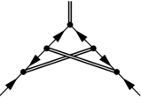
a)         b)

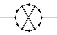
Figure 4: a) A typical higher-order correction to the quark-diquark vertex. b) Corresponding higher-order correction to the diquark propagator, which is discarded in this paper.

A consistent treatment of the baryon would then require to include the same correction into the diquark propagator. This complicated procedure which goes beyond the one-loop expression for the diquark propagator is clearly outside the scope of this paper.

Let us remark that in the case of light quarks the class of diagrams shown in Fig. 2 just represents the minimal subset of diagrams which is required to fulfill the Pauli-principle in the quark-diquark picture of baryons [22, 24]. The above series of diagrams defines a kind of ladder approximation which in the next step will be summed up to yield a Faddeev type of 3-body amplitude. Hereby, the presence of both light and heavy diquarks induces a $2\!\times\!2$ matrix structure. Therefore, we introduce the matrix of the free quark–diquark propagation $G={\rm diag}\left(G_{XX},\,G_{YY}\right)$,

$$(G_{XX})^{\beta\beta^{\prime}}(x,x^{\prime};\,y,y^{\prime}) = i\ D^{\beta\beta^{\prime}}(x^{\prime},y^{\prime})\ g_{v}(x,y)\ ,$$

$$(G_{YY})^{{\beta_{0}}{\beta_{0}}^{\prime}}_{ij\ i^{\prime}j^{\prime}}(x,x^{\prime};\,y,y^{\prime}) = i(D_{v})^{{\beta_{0}}{\beta_{0}}^{\prime}}_{jj^{\prime}}(x^{\prime},y^{\prime})(g_{0})_{ii^{\prime}}(x,y)\ .$$ (27)

Here, $g_{v}$ and $g_{0}$ denote the free propagators of heavy and light constituent quarks, respectively. Now we define the interaction matrix $H$, whose elements mediate the transitions ${\cal X}_{v}\leftrightarrow{\cal Y}_{v}$ and ${\cal Y}_{v}\to{\cal Y}_{v}$. As can be read off from Fig. 2 by straightening the diquark lines, these transitions are mediated by quark–exchange. In Fig. 5 the elements of $H$ are depicted graphically. We have:

$$H = \left(\begin{array}[]{cc}0&H_{XY}\\ H_{YX}&H_{YY}\end{array}\right)\ ,$$ (30)

$$(H_{XY})^{\beta{\beta_{0}}^{\prime}}_{\ \ i^{\prime}j^{\prime}}(x,x^{\prime};\,y,y^{\prime}) = \frac{1}{2}\ \Gamma_{v}^{{\beta_{0}}^{\prime}}\ (\tilde{g}_{0}(x,y)\Gamma^{\beta})_{j^{\prime}i^{\prime}}\ \delta(x^{\prime}-y)\ \delta(y^{\prime}-x)\ ,$$

$$(H_{YX})^{{\beta_{0}}\beta^{\prime}}_{ij}(x,x^{\prime};\,y,y^{\prime}) = \frac{1}{2}\ (\Gamma^{\beta^{\prime}}\tilde{g}_{0}(x,y))_{ij}\ \Gamma_{v}^{{\beta_{0}}}\ \delta(x^{\prime}-y)\ \delta(x-y^{\prime})\ ,$$

$$(H_{YY})^{{\beta_{0}}{\beta_{0}}^{\prime}}_{ij\ i^{\prime}j^{\prime}}(x,x^{\prime};\,y,y^{\prime}) = \frac{1}{4}\,\tilde{\Gamma}_{v}^{{\beta_{0}}^{\prime}}\ \tilde{g}_{v}(x,y)\ \tilde{\Gamma}_{v}^{{\beta_{0}}}\ \delta(x^{\prime}-y)\ \delta(x-y^{\prime})\ \delta_{ji^{\prime}}\,\delta_{ij^{\prime}}\ .$$ (31)

$H_{XY}$	$H_{YX}$	$H_{YY}$

Figure 5: Elements of the interaction matrix $H$.

Here, $\tilde{\Gamma}_{v}\ =\ C^{\dagger}\ \Gamma_{v}^{T}\ C$. Note that $H_{YY}$ formally mediates the exchange of the heavy quark. With the above definitions of $G$ and $H$, the baryon propagator defined by the series of diagrams shown in Fig. 2 becomes:

$$\langle G_{B}\rangle=G\ \sum_{k}(H\ G)^{k}=\ G\ (1-H\ G)^{-1}\ .$$ (32)

It has the standard form of a Faddeev type of 3–particle propagator.

3 The Faddeev equation

Baryon masses are given by the poles of the baryon propagator (32), which results in a Faddeev type of equation for the baryon wave functions:

$$(1-G\,H)\ \left(\begin{array}[]{c}{\cal X}_{v}\\ {\cal Y}_{v}\end{array}\right)=0\ .$$ (33)

Figure 6: Graphical representation of the Faddeev equation for heavy baryons.

For the solution of this equation it is convenient to switch to momentum space. Denoting the total momentum of the baryon (with $m_{Q}v$ subtracted according to the phase factor in (1)) by $p$ and the relative momentum by $2q$, $2k$, respectively, we obtain (see Fig. 6):

$${\cal X}_{v}^{\alpha}(p,q) = \frac{i}{2}\,\int_{k}\ D^{\alpha\alpha^{\prime}}(p_{-})\ g_{v}(p_{+})\ \Gamma_{v}^{{\beta_{0}}}\,(\tilde{g}_{0}(k+q)\ \Gamma^{\alpha^{\prime}})_{ji}\ {{\cal Y}_{v}}_{ij}^{\beta_{0}}(p,k)\ ,$$ (34)

$${{\cal Y}_{v}}_{ij}^{\alpha_{0}}(p,q) = \frac{i}{2}\ \int_{k}\ (D_{v})^{{\alpha_{0}}{\alpha_{0}}^{\prime}}_{jj^{\prime}}(p_{-})\ (g_{0})_{ii^{\prime}}(p_{+})\ (\Gamma^{\beta}\ \tilde{g}_{0}(k+q))_{i^{\prime}j^{\prime}}\ \Gamma_{v}^{{\alpha_{0}}^{\prime}}\ {\cal X}_{v}^{\beta}(p,k)$$ (35)

$$+ \frac{i}{4}\ \int_{k}\ (D_{v})^{{\alpha_{0}}{\alpha_{0}}^{\prime}}_{jj^{\prime}}(p_{-})\ (g_{0})_{ii^{\prime}}(p_{+})\ \tilde{\Gamma}_{v}^{{\beta_{0}}}\ \tilde{g}_{v}(k+q)\ \tilde{\Gamma}_{v}^{{\alpha_{0}}^{\prime}}\ {{\cal Y}_{v}}^{\beta_{0}}_{j^{\prime}i^{\prime}}(p,k)\ .$$

Here $p_{+}$ and $p_{-}$ are abbreviations for $(p/2+q)$ and $(p/2-q)$, respectively, and $\int_{k}$ stands for $\int d^{4}k/(2\pi)^{4}$. Note that in momentum space one has $\tilde{g}_{0}(k+q)=C^{\dagger}g_{0}^{T}(-(k+q))C$ (here, the transpose refers to Dirac indices only). In the following, we will restrict ourselves to the lowest lying diquark states, namely the scalar and axial-vector diquark channel.

Furthermore, we will not perform a full dynamical calculation of the Faddeev amplitudes, which would require a tremendous amount of numerical work. Instead, we will consider the diquarks as point-like bosons. This reduces the Faddeev equation (34), (35) to a Bethe–Salpeter type of equation. For the light diquarks, we use Klein–Gordon propagators $D(k^{2})=Z[k^{2}-M^{2}]^{-1}$, with masses M = ${M_{s},M_{a}}$ and wave function renormalization factors $Z={Z_{s},Z_{a}}$, where the indices refer to scalar and axial–vector diquarks, respectively.

Accordingly, for the heavy diquarks we use the propagator of a free bosonic field which has been subject to the heavy quark transformation (1):

$$(D_{v})^{{\beta_{0}}{\beta_{0}}^{\prime}}_{jj^{\prime}}(v\!\cdot\!k)=\frac{Z_{j}}{v\!\cdot\!k-\Delta M_{j}+i\epsilon}\ \delta^{{\beta_{0}}{\beta_{0}}^{\prime}}\,\delta_{jj^{\prime}}\quad\times\quad\Big{\{}\begin{array}[]{cc}1&\mbox{for scalar diquarks}\\ g_{\mu\mu^{\prime}}-v_{\mu}v_{\mu^{\prime}}&\mbox{for axial--vector diquarks}\end{array}\ .$$

Here, $\Delta M=M-m_{Q}$ is the residual diquark mass and $Z$ denotes the wave function renormalization factor. The heavy scalar and axial vector diquarks are degenerate due to the heavy quark spin symmetry. The diquark masses and $Z$–factors appearing in the above expressions are calculated using eqs. (22) and (23) (see appendix B for details). Numerical values are given in section 4.

The color structure of the interaction matrices $H$ can conveniently be rewritten in terms of the color projection operators onto singlet and octet states:

$$H^{AB}_{CE}\ \sim\ \frac{i\,\epsilon^{B}_{CD}}{\sqrt{2}}\ \ \frac{i\,\epsilon^{A}_{DE}}{\sqrt{2}}\ =\ -{}^{(1)}P_{CE}^{AB}\ +\ \frac{1}{2}\ {}^{(8)}P_{CE}^{AB}\ \ ,\quad{}^{(1)}P_{CE}^{AB}=\frac{1}{3}\delta^{A}_{C}\ \delta^{B}_{E}\,.$$

Then eqs. (34), (35) can be shown to decouple in color space and the parts describing the relevant color singlet amplitudes can be identified.
In the case of exact flavor symmetry, the flavor structure of eqs. (34), (35) is trivial, since all propagators are proportional to the unit matrix in the (light) flavor space. Then the flavor matrices $t_{ij}^{a}$ connected with the fields ${\cal X}^{a}$ project out either the symmetric ($6_{F}$) or the anti–symmetric ($\bar{3}_{F}$) flavor part of ${\cal Y}_{ij}$, respectively, which leads to a total decoupling of $6_{F}$ and $\bar{3}_{F}$ amplitudes.
The explicit breaking of the $SU(3)_{F}$ flavor symmetry induces a mixing of these amplitudes. As a first approximation we will keep the flavor structure in the kernel of eqs. (34), (35), but neglect the mixing effects for the amplitudes. The error involved is of first order in $(m_{s}-m_{u})$ for the baryon wave functions, i.e. of second order for the mass spectrum.

Furthermore, we are interested only in ground state baryons, which are given by s–wave (quark–diquark) amplitudes as discussed in [27]. For s–wave baryons, the transversal momentum of the exchanged quark should be of minor importance and will be neglected. This approximation implies the replacement:

$$k\!\!\!/\longrightarrow(v\!\cdot\!k)\,v\!\!\!/\quad\Rightarrow\quad\tilde{g}_{0}(k)\ \to\ \frac{1}{-v\!\cdot\!k-m+i\epsilon}\ ,$$ (36)

where the relations $\frac{1+v\hskip-3.5pt/}{2}{\cal X}_{v}={\cal X}_{v}$ and $\Gamma_{v}\ \frac{1+v\hskip-3.5pt/}{2}=\frac{1-v\hskip-3.5pt/}{2}\ \Gamma_{v}$ were used. Now we insert (36) into eqs. (34), (35) and perform the integration over the relative momentum $q$, defining ${\cal X}(p)=\int_{q}{\cal X}_{v}(p,q)$ and ${\cal Y}_{v}(p)=\int_{q}{\cal Y}_{v}(p,q)$. This leads to a decoupling of the terms $\frac{1-v\hskip-3.5pt/}{2}\ {\cal Y}_{v}$ and the longitudinal parts $v_{\mu}{\cal X^{\mu}}$ (where ${\cal X^{\mu}}$ denotes an amplitude containing an axial–vector diquark). Therefore, the equations now enforce the Bargmann–Wigner condition, i.e. to leading order in $1/m_{Q}$ the baryon amplitudes are eigenstates of the projector $\frac{1+v\hskip-3.5pt/}{2}$, and the transversality condition (3) is fulfilled (see [27] for more details about these conditions).

Finally, linear combinations of the baryon amplitudes have to be found which are eigenstates of projection operators onto spin 1/2 and spin 3/2. For this purpose, we introduce the following set of spin projection operators:

$$t_{\mu} = \frac{1}{\sqrt{3}}(\gamma_{\mu}-v\hskip-5.0pt/v_{\mu})\ ,\quad v^{\mu}t_{\mu}\ =\ 0\ ,$$

$${}^{\left[3/2\right]}P_{\mu\nu} = \ g_{\mu\nu}\ -\ v_{\mu}v_{\nu}\ -\ t_{\mu}t_{\nu}\ ,\quad v_{\mu}{}^{\left[3/2\right]}P^{\mu\nu}=\gamma_{\mu}{}^{\left[3/2\right]}P^{\mu\nu}\ =\ 0\ .$$ (37)

Here, ${}^{\left[3/2\right]}P_{\mu\nu}$ projects onto spin 3/2 while $t_{\mu}t_{\nu}$ projects onto the part of spin 1/2 which is transversal with respect to $v_{\mu}$. The Dirac structure in (34), (35) stemming from the interaction vertices can now be rearranged as

$$O^{{\sf a}^{\prime}}_{v}\,\times\,O^{{\sf a}}_{v} = \left\{\gamma_{5},\ \gamma_{\nu}-v_{\nu}v\hskip-5.0pt/\right\}^{{\sf a}^{\prime}}\,\times\,\left\{\begin{array}[]{c}\gamma_{5}\\ \gamma_{\mu}-v_{\mu}v\hskip-5.0pt/\end{array}\right\}^{{\sf a}}\ =\ \left\{\begin{array}[]{cc}1&\sqrt{3}t_{\nu}\gamma_{5}\\ \sqrt{3}\gamma_{5}t_{\mu}&2\ {}^{\left[3/2\right]}P_{\mu\nu}-t_{\mu}t_{\nu}\end{array}\right\}^{{\sf a}{\sf a}^{\prime}}\ .$$ (42)

The system of integral equations (34), (35) can then be diagonalized with respect to the spin structure by introducing the following linear combinations:

$${}^{\left[1/2\right]}{\cal X}_{v} := {\cal X}_{v}\ ,$$

$${}^{\left[1/2\right]}{\cal X}_{v}^{\prime} := \frac{1}{\sqrt{2}}\ t_{\mu}\gamma_{5}{\cal X}_{v}^{\mu}\ ,$$

$${}^{\left[3/2\right]}{{\cal X}_{v}^{*}}^{\mu} := \frac{1}{\sqrt{2}}\ {}^{\left[3/2\right]}P^{\mu}_{\nu}{\cal X}_{v}^{\nu}\ .$$ (43)

and

$${}^{\left[1/2\right]}{\cal Y}_{v} := \frac{1}{2}({\cal Y}_{v}+\sqrt{3}t_{\nu}\gamma_{5}{\cal Y}_{v}^{\nu})\ ,$$

$${}^{\left[1/2\right]}{\cal Y}_{v}^{\prime} := \frac{1}{2}(\sqrt{3}{\cal Y}_{v}+t_{\nu}\gamma_{5}{\cal Y}_{v}^{\nu})\ ,$$

$${}^{\left[3/2\right]}{{\cal Y}_{v}^{*}}^{\mu} := {}^{\left[3/2\right]}P^{\mu}_{\nu}{\cal Y}_{v}^{\nu}\ .$$ (44)

Note that in the case of ${}^{\left[1/2\right]}{\cal Y}_{v}$ and ${}^{\left[1/2\right]}{\cal Y}_{v}^{\prime}$ both the heavy scalar and heavy axial vector diquarks contribute.
Now eqs. (34), (35) can be decomposed into two separate sets of coupled equations for the baryons with the light flavors in the $\bar{3}_{F}$ representation ($\Lambda_{Q}$, $\Xi_{Q}$) and the $6_{F}$ representation ($\Sigma_{Q}^{(*)}$, $\Xi_{Q}^{\prime}{}^{(*)}$, $\Omega_{Q}^{(*)}$), respectively. The equations for the fields ${}^{\left[3/2\right]}{{\cal X}_{v}^{*}}^{a}$, ${}^{\left[3/2\right]}{{\cal Y}_{v}^{*}}_{ij}$ indeed turn out to be identical to those for the fields ${}^{\left[1/2\right]}{{\cal X}_{v}^{\prime}}^{a}$, ${}^{\left[1/2\right]}{{\cal Y}_{v}^{\prime}}_{ij}$ which reflects the degeneracy due to the heavy quark spin symmetry.
The fact that the system is now diagonal with respect to the flavor and the spin content shows that the Pauli principle (which was inherent in the amplitude ${\cal X}_{v}$ containing the light diquark) is established dynamically in the amplitude ${\cal Y}_{v}$. As shown above, the physical baryon which will be a linear combination of ${\cal X}_{v}$ and ${\cal Y}_{v}$, always has a definite relation between flavor and spin quantum numbers.

4 Numerical results

Even with the simplifications introduced in the previous section, a complete solution of the resulting coupled integral equations for the baryon amplitudes ${\cal X}_{v}(p),{\cal Y}_{v}(p)$ would be a rather complicated numerical task.
To get a first rough estimate of the baryon spectrum, we apply an even stronger final approximation which has proven to work quite well in the light baryon sector (compare [30, 31, 32]). This approximation implies the neglect of the total momentum dependence of the exchanged quark in $H$, i.e. $g_{0}(k)\ \rightarrow\ -1/m$ with $m$ being the light quark mass, and is referred to as a static approximation. Here, we will use the same approximation also for the propagator of the exchanged heavy quark, since, as can be seen from eq. (36), it differs from the light quark propagator only by a constant shift in the relative momentum of the amount $mv^{\mu}$. This shift can be absorbed into the definition of the wave functions entering eqs. (34), (35).

With these approximations for the exchanged quarks, the integral equations (34), (35) for the baryon amplitudes become a set of completely decoupled algebraic equations for the masses of spin 1/2 baryons in the $\bar{3}_{F}$ representation and for those in the $6_{F}$ representation, the latter including the spin 3/2 baryons. The final equations are of the form

$$\frac{4}{(F_{ij}+F_{ji})}\ -\ {F^{[s]}}_{ij}\ =\ 1\ .$$ (45)

where $F_{ij}(vp)$ and $F^{[s]}_{ij},s=1/2,\ 3/2$, defined in appendix B, are integrals over the relative momentum of the quark and diquark propagators. These integrals are UV–divergent. In a complete analysis of eqs. (34), (35), the integration over the relative momentum $q$ would be limited to the width of the wave–function appearing in the integral, which would render the integration UV–finite (compare e.g. [33]). Here, we will employ an UV–regularization for the quark–diquark relative momentum integrals, where for simplicity the same method will be used as in the calculation of the diquark masses (see appendix B).

The usual NJL model parameters are fixed in the light pseudoscalar meson sector and the light baryon sector. For the latter we refer to the NJL model calculation in [31]. In this work, a constituent mass of $m_{u}=m_{d}=450$ MeV was used, from which the NJL cut–off and the strange quark constituent mass are calculated by a fit to the light meson spectrum, resulting in $\Lambda=630$ MeV and $m_{s}=650$ MeV. Moreover, there it was found that the coupling constant for the light axial vector diquark has to be increased relative to that of the scalar sector: $G_{1a}=1.5\ G_{1}$. In the following, the value of the coupling constant in the heavy sector $G_{3}$ is left equal to that of $G_{1}$. For convenience, the corresponding mesonic coupling constant $G_{\rm meson}=19.4\ \Lambda^{-2}$ from the above fit is used as a normalization for $G_{1}$.

First, some diquark masses for different values of $G_{1}$ are presented in Table 1. The results for the masses of heavy diquarks are similar to those of heavy mesons [12].

$G_{1}/G_{\rm meson}$	$M_{s}^{\left[u,d\right]}$	$M_{s}^{\left[u,s\right]}$	$M_{a}^{\left\{u,d\right\}}$	$M_{a}^{\left\{u,s\right\}}$	$M_{a}^{\left\{s,s\right\}}$	$\Delta M_{u}$	$\Delta M_{s}$
1.1	705	895	875	1050	1215	360	530
1.2	680	870	865	1035	1200	345	520
1.3	650	845	855	1020	1185	330	505
1.4	620	820	845	1010	1170	320	495
1.5	595	795	835	1000	1160	305	480

Table 1: Light scalar and axial vector diquark masses and heavy diquark masses (all in MeV) for $m_{u}=450$ MeV, $m_{s}=650$ MeV, $\Lambda=630$ MeV, $G_{3}=G_{1}$, $G_{1a}=1.5\,G_{1}$, $G_{\rm meson}=19.4~{}\Lambda^{-2}$.

Figure 7: Light diquark masses $M_{s}$, $M_{a}$, heavy diquark residual masses $\Delta M$ and heavy baryon residual masses $\Delta M_{\Lambda_{Q}}$, $\Delta M_{\Sigma_{Q}}$ as functions of the coupling strength. The mass splitting between $\Lambda_{c}$ and $\Sigma_{c}$ found in experiment is marked with an arrow.

In Fig. 7, diquark masses and residual masses of the non–strange heavy baryons $\Lambda_{Q}$ and $\Sigma_{Q}$ following from eq. (45) are shown as a function of the coupling constant $G_{1}$. The circles indicate the masses of the diquarks found in the fit to the light baryons [31] which determines the parameter range to be used in the following as $G_{1}/G_{\rm meson}=1.2-1.3$. Indeed, here we find a reasonable mass–splitting of 160–175 MeV for the heavy baryons $\Lambda_{Q}$ and $\Sigma_{Q}$. The experimental value for the charmed baryons is $M_{\Sigma_{c}}-M_{\Lambda_{c}}=170$ MeV which is indicated with an arrow in Fig. 7.
The following masses of charmed baryons have been determined so far [34, 35]:

$$\Lambda_{c}(2285)\ ,\quad\Sigma_{c}(2455)\ ,\quad\Xi_{c}(2470)\ ,\quad\Omega_{c}(2705)\ ,\quad\Xi_{c}^{*}(2644).$$

In the bottom sector only the data for $\Lambda_{b}(5641)$ [34] is reliable up to now.
Our results in Table 2 were obtained without changing the parameter set used for the calculation of light meson and baryon spectra in [31]. For a value of $G_{1}=1.3\ G_{\rm meson}$, the mass splittings $\Sigma_{c}-\Lambda_{c}$ and $\Xi_{c}-\Lambda_{c}$ obviously agree quite well with the experimental data. Note that the (preliminary) result $\Sigma_{b}-\Lambda_{b}=173$ MeV [36] equals the corresponding mass splitting in the charmed sector. The $\Omega_{c}-\Lambda_{c}$ splitting comes out somewhat too large, whereas the splitting $\Xi_{c}^{\ast}-\Xi_{c}$ is somewhat too small.
However, our calculation without $1/m_{Q}$ corrections cannot account precisely for the mass splittings within the $6_{F}$ multiplets. Using spin–weighted averages for these multiplets (with preliminary results or estimates [37] for the candidates not yet determined) would significantly improve our predictions for $\{\Xi^{\prime},\Xi^{*}\}$ and $\{\Omega,\Omega^{*}\}$ (whereas the prediction for $\{\Sigma^{\prime},\Sigma^{*}\}$ would probably be somewhat too small then). But a definite analysis requires more reliable experimental data, and perhaps even a re–analysis of the so far performed classification of heavy baryon states [38].

$G_{1}/G_{\rm meson}$	$\Sigma_{Q}-\Lambda_{Q}$	$\Xi_{Q}-\Lambda_{Q}$	$\Omega_{Q}-\Lambda_{Q}$	$\Xi^{\ast}_{Q}-\Xi_{Q}$
1.20	162	192	495	136
1.30	175	198	513	146
1.40	189	204	531	156
Exp.:	170	185	420	174

Table 2: Heavy baryon mass splittings in MeV. The NJL coupling constant $G_{1}$, which triggers the diquark properties, is given in units of the coupling constant of the (light) pseudoscalar meson sector.

5 Summary and outlook

In this work we have derived the Faddeev equations for heavy baryons in the quark–diquark picture, starting from a current–current interaction of the NJL–type model, where heavy quarks have been included in the heavy mass limit.

After extensive use of functional integration techniques, the baryon propagator has been obtained as a series of quark exchange diagrams, which could be summed up to yield the bound state equations for the baryon wave functions.

An essential feature of our approach is that two different types of quark–diquark configurations contribute to the baryon wave functions: One, where a heavy quark is coupled to a light diquark, and the other where a heavy diquark is coupled to a light quark. The properties of the heavy diquark are also fixed by the underlying NJL model and discussed in some detail, showing a similar mass pattern as in the case of heavy mesons.

For a further analysis of the baryon bound state equations, we approximated the diquarks as point-like particles, which reduces the Faddeev equations to effective Bethe–Salpeter type of equations. In an s–wave approximation (that means in our case to neglect the transversal momentum part of the interaction), the Bargmann–Wigner condition and the transversality condition for the heavy baryon wave functions are fulfilled exactly. Projecting onto color singlet states and defining the proper spin projections, we then observe a decoupling of the equations for suitably chosen linear combinations of wave functions. They describe the predicted multiplets of heavy quark spin symmetry: the lowest–lying spin 1/2 state (a $\bar{3}_{F}$ multiplet in the light flavor’s $SU(3)_{F}$) and the spin 1/2 state (a $6_{F}$ multiplet) which is degenerate with the spin 3/2 state.

The Pauli principle for the two light quarks inherent in the light diquark system is established dynamically for the baryon wave functions: We have shown that in the $SU(3)_{F}$ limit baryonic states (with definite spin) where the light quarks are in the $\bar{3}_{F}$–representation do not mix with those states where the light quarks belong to the $6_{F}$ multiplet. This feature is preserved even if $SU(3)_{F}$ breaking is included in leading order.

For a numerical estimate of the mass spectrum, a static approximation for the quark–diquark interaction was found, which treats both heavy and light quark exchange on an equal footing and leads to analytically solvable equations. By applying a parameter fit obtained from the light baryon spectrum, we then arrived at reasonable masses for the ground state heavy baryons.

As we have shown in ref. [39], the quark–diquark picture is also useful to estimate the coupling of heavy baryons to pions and weak heavy quark currents, defining the Isgur–Wise form factors. The results of the present work are to be extended in this direction in the future.

Appendix A Deriving the effective baryon lagrangian

After inserting the functional constants (11)–(14) into the generating functional, the effective action reads:

$$S_{\rm eff} = \int_{x,y}\bar{q}\ (i\ \partial\!\!\!/-m)\ q\ +\ \bar{Q}_{v}\ (iv\cdot\partial)\ Q_{v}\$$

$$- \frac{1}{2}\int_{x,y}\left(\bar{q}\ \Delta^{\alpha}\ \Gamma^{\alpha}\ q^{c}\ +\ \bar{q}^{c}\ \Delta^{\dagger\ \alpha}\ \Gamma^{\alpha}\ q\ +\ \bar{Q}_{v}\Gamma^{{\alpha_{0}}}_{v}\ \Delta_{v}^{{\alpha_{0}}}q^{c}\ +\ \bar{q}^{c}\ \Gamma^{{\alpha_{0}}}_{v}\Delta_{v}^{\dagger\ {\alpha_{0}}}Q_{v}\right)$$

$$- \int_{x}\left[\frac{1}{8G_{1}}\Delta^{\dagger\ \alpha}(x)\Delta^{\alpha}(x)\ -\int_{y}\bar{Q}_{v}(y)X^{\alpha}(y,x)\Delta^{\dagger\ \alpha}(x)\right]$$

$$+ \int_{x,y}\left[\Delta^{\alpha}(x)\bar{X}^{\alpha}(y,x)Q_{v}(y)\ -\ 8G_{1}\int_{y^{\prime}}\bar{Q}_{v}(y^{\prime})X^{\alpha}(y^{\prime},x)\bar{X}^{\alpha}(y,x)Q_{v}(y)\right]$$

$$- \int_{x}\left[\frac{1}{4G_{3}}\ \Delta_{v}^{{\alpha_{0}}}(x)\Delta_{v}^{\dagger\ {\alpha_{0}}}(x)\ -\int_{y}\bar{q}(y)\ t^{a}\ Y^{\alpha}(y,x)\Delta^{\dagger\ {\alpha_{0}}}_{v}(x)\right]$$

$$+ \ \int_{x,y}\left[\Delta^{{\alpha_{0}}}_{v}(x)\bar{Y}^{\alpha}(y,x)\ t^{a}\ q(y)\ -\ 4G_{3}\int_{y^{\prime}}\bar{q}(y)\ t^{a}\ Y^{\alpha}(y,x)\bar{Y}^{\alpha}(y^{\prime},x)\ t^{a}\ q(y^{\prime})\right]$$

$$+ \int_{x,y}\bar{X}\ {\cal X}\ +\ \bar{\cal X}\ X\ +\ \bar{Y}\ {\cal Y}\ +\ \bar{\cal Y}\ Y\ .$$

The heavy quark fields are removed from the generating functional by a simple Gaussian integration. For the terms containing light quark fields we employ the Nambu-Gorkov formula:

$$\int D\bar{q}\ Dq\ \exp\ i\left[\ \frac{1}{2}\int_{x,y}(\bar{q},\ q^{T})\left(\begin{array}[]{cc}A&B\\ C&D\end{array}\right)\left(\begin{array}[]{c}q\\ \bar{q}^{T}\end{array}\right)\ \pm\ \frac{1}{2}\int_{x}(\bar{q}\eta\ +\ \bar{\eta}q)\right]$$ (A.6)

$$= \exp\left[\frac{1}{2}{\rm Tr\ log}\left(\begin{array}[]{cc}A&B\\ C&D\end{array}\right)\ -\frac{i}{8}(\bar{\eta},\ -\eta^{T})\left(\begin{array}[]{cc}A&B\\ C&D\end{array}\right)^{-1}\left(\begin{array}[]{c}\eta\\ -\bar{\eta}^{T}\end{array}\right)\right]\ ,$$ (A.13)

were in our case the components read:

$$A(x,y) = (i\partial\!\!\!/-m)\delta(x-y)\ -\ 4G_{3}\ \int_{z}t^{a}\ Y_{a{\alpha_{0}}}(x,z)\bar{Y}_{a^{\prime}{\alpha_{0}}}(y,z)\ t^{a^{\prime}}$$

$$+ \frac{1}{4}\left[C\ \Delta_{v}^{\dagger}(y)\ S_{v}(y,x)\ \Delta_{v}(x)C\right]^{T}$$

$$B(x,y) = -\Delta(x)\delta(x-y)\ C\ ,$$

$$C(x,y) = -C\ \tilde{\Delta}(x)\delta(x-y)\ ,$$

$$D(x,y) = -A^{T}(x,y)$$

$$\eta(x) = 2\ t^{a}\ \int_{z}Y^{\alpha}(x,z)\ \Delta_{v}^{\dagger\ {\alpha_{0}}}$$

$$- \left[\int_{x^{\prime},z}\bar{X}^{\alpha^{\prime}}(x^{\prime},z)\Delta^{\alpha^{\prime}}(z)\ S_{v}(x^{\prime},x)\ \Delta_{v}(x)\ C\right]^{T}$$

$$\bar{\eta}(x) = 2\int_{z}\Delta_{v}^{{\alpha_{0}}}(z)\bar{Y}^{\alpha}(x,z)\ t^{a}$$ (A.14)

$$- \left[\int_{y,z}C\ \tilde{\Delta}_{v}(x)\ S_{v}(x,y)\ \Delta^{\dagger\ \alpha^{\prime}}(z)X^{\alpha^{\prime}}(y,z)\right]^{T}\ .$$

Here, Tr denotes the trace over all indices, including space-time indices. We define the inverse of the following matrix

$$\left(\begin{array}[]{cc}A&B\\ C&D\end{array}\right)^{-1}=:\left(\begin{array}[]{cc}g_{11}&g_{12}\\ g_{21}&g_{22}\end{array}\right)$$

and the quantity

$$S_{v}^{-1}(x,y):=(iv\cdot\partial)\frac{1+v\hskip-5.0pt/}{2}\delta(x-y)\ -\ 8\,G_{1}\int_{a}\ X^{\alpha}(x,a)\ \bar{X}^{\alpha}(y,a)\ .$$ (A.15)

Note that the projection operator $\frac{1+v\hskip-3.5pt/}{2}$ is always present next to a $Q_{v}$ or $X_{v}$ field.

The effective action now reads:

$$i\ S_{\rm eff} = -\frac{i}{8G_{1}}\int\ \Delta^{\dagger\ \alpha}\Delta^{\alpha}\ -\ \frac{i}{4G_{3}}\int\ \Delta_{v}^{{\alpha_{0}}}\Delta^{\dagger\ {\alpha_{0}}}_{v}\ +\ Tr\ log\ S_{v}^{-1}$$

$$+ \frac{1}{2}{\rm Tr\ log}\left(\begin{array}[]{cc}A&B\\ C&D\end{array}\right)\ -\ \frac{i}{8}(\bar{\eta},\ -\eta^{T})\left(\begin{array}[]{cc}g_{11}&g_{12}\\ g_{21}&g_{22}\end{array}\right)\left(\begin{array}[]{c}\eta\\ -\bar{\eta}^{T}\end{array}\right)$$

$$- i\ \int_{x,y,a,a^{\prime}}\bar{X}^{\alpha}(x,a)\Delta^{\alpha}(a)\ S_{v}(x,y)\ \Delta^{\dagger\ \alpha}(a^{\prime})\ X^{\alpha}(y,a^{\prime})$$

$$+ \int_{x,y}\bar{X}\ {\cal X}\ +\ \bar{\cal X}\ X\ +\ \bar{Y}\ {\cal Y}\ +\ \bar{\cal Y}\ Y\ .$$ (A.23)

Expanding this expression up to second order in the baryon fields, we obtain the entries for the matrix $G_{B}$ defined in (19) as given by

$$(G_{B\ XX})^{\beta\beta^{\prime}}(x,x^{\prime};\,y,y^{\prime})=\Delta^{\beta}(x^{\prime})\ g_{v}(x,y)\ {\Delta^{\dagger}}^{\beta^{\prime}}(y^{\prime})$$

$$\qquad+\frac{1}{4}\,\int d^{4}a\,d^{4}z\ \Delta^{\beta}(x^{\prime})\ g_{v}(x,z)\ {\Delta_{v}}_{k}(z)\ C\,g_{22}(z,a)_{kl}\,C\ {\Delta_{v}^{\dagger}}_{l}(a)\ g_{v}(a,y)\ {\Delta^{\dagger}}^{\beta^{\prime}}(y^{\prime})\ ,$$

$$(G_{B\ XY})^{\beta{\beta_{0}}^{\prime}}_{\ i^{\prime}j^{\prime}}(x,x^{\prime};\,y,y^{\prime})=\frac{1}{2}\,\int d^{4}a\ \Delta^{\beta}(x^{\prime})\ g_{v}(x,a)\ {\Delta_{v}}_{k}(a)\ C\,g_{21}(a,y)_{ki^{\prime}}\ {\Delta_{v}^{\dagger}}_{j^{\prime}}^{{\beta_{0}}^{\prime}}(y^{\prime})\ ,$$

$$(G_{B\ YX})^{{\beta_{0}}\beta^{\prime}}_{ij}(x,x^{\prime};\,y,y^{\prime})=\frac{1}{2}\,\int d^{4}a\ {\Delta_{v}}_{j}^{{\beta_{0}}}(x^{\prime})\ g_{12}(x,a)_{il}\,C\ {\Delta^{\dagger}_{v}}_{l}(a)\ g_{v}(a,y)\ {\Delta^{\dagger}}^{\beta^{\prime}}(y^{\prime})\ ,$$

$$(G_{B\ YY})^{{\beta_{0}}{\beta_{0}}^{\prime}}_{ij\,i^{\prime}j^{\prime}}(x,x^{\prime};\,y,y^{\prime})={\Delta_{v}}_{j}^{{\beta_{0}}}(x^{\prime})\ g_{11}(x,y)_{ii^{\prime}}\ {\Delta_{v}^{\dagger}}_{j^{\prime}}^{{\beta_{0}}^{\prime}}(y^{\prime})\ ,$$ (A.24)

where

$$g_{11} = (1-g\ \Delta\ \tilde{g}\ \Delta^{\dagger})^{-1}g\ ,$$

$$g_{22} = -g_{11}^{T}$$

$$g_{12} = (1-g\ \Delta\ \tilde{g}\ \Delta^{\dagger})^{-1}g\ \Delta\ \tilde{g}\ C^{\dagger}\ ,$$

$$g_{21} = C^{\dagger}(1-\tilde{g}\ \Delta^{\dagger}\ g\ \Delta)^{-1}\ \tilde{g}\ \Delta^{\dagger}\ g\ .$$ (A.25)

The expression $\tilde{g}$ is defined as $\tilde{g}\ =\ C^{\dagger}\ g^{T}\ C$, where $\left\{\right\}^{T}$ means ’transposed in all indices’ (including coordinate space). Note that the Dyson expansions for the terms $g_{ii}$ yield quark–diquark contributions up to any order.

Appendix B Calculation of integrals in the proper–time scheme

As far as the integrals (in momentum space) for the diquark propagators (22) and (23) are concerned, the proper-time regularization procedure is applied to the quark determinant appearing in (19), such that Ward-Identities are respected. The essential techniques are outlined in [40]. For the integrals with one heavy and one light particle in the loop, the basic replacement reads (after Wick-rotation):

$$\frac{1}{q^{2}+m^{2}}\ =\int_{0}^{\infty}ds\ e^{-s(q^{2}+m^{2})}\ \longrightarrow\int_{\frac{1}{\Lambda^{2}}}^{\infty}ds\ e^{-s(q^{2}+m^{2})}\ .$$ (B.1)

We define

$$I^{1}(m^{2}) := \frac{i}{(2\pi)^{4}}\,\int^{reg}\,\frac{d^{4}q}{q^{2}-m^{2}+i\epsilon}\ =\ \frac{m^{2}}{16\pi^{2}}\,\Gamma(-1,\frac{m^{2}}{\Lambda^{2}})\ ,$$ (B.2)

$$I^{2}(m^{2}) := -\frac{i}{(2\pi)^{4}}\,\int^{reg}\,\frac{d^{4}p}{(p^{2}-m^{2}+i\epsilon)^{2}}\ =\ \frac{1}{16\pi^{2}}\,\Gamma(0,\frac{m^{2}}{\Lambda^{2}})\ ,$$ (B.3)

$$I^{3}_{m}(v\!\cdot\!p) := -\frac{i}{(2\pi^{4})}\,\int^{reg}\,\frac{d^{4}q}{(q^{2}-m^{2}+i\epsilon)\,(v\!\cdot\!q+v\!\cdot\!p+i\epsilon)}$$ (B.4)

$$= \ \ \frac{\sqrt{\pi}}{16\pi^{2}}\,\sqrt{m^{2}-(v\!\cdot\!p)^{2}}\,\Gamma(-\frac{1}{2},\frac{m^{2}-(v\!\cdot\!p)^{2}}{\Lambda^{2}})$$

$$+\frac{v\!\cdot\!p}{16\pi^{2}}\,\int_{0}^{1}\,\frac{dx}{\sqrt{1-x^{2}}}\,\Gamma(0,\frac{m^{2}-x(v\!\cdot\!p)^{2}}{\Lambda^{2}})\ ,$$

$$I^{4}_{m}(v\!\cdot\!p) := -\frac{i}{(2\pi^{4})}\,\int^{reg}\,\frac{d^{4}q}{(q^{2}-m^{2}+i\epsilon)\,(v\!\cdot\!q+v\!\cdot\!p+i\epsilon)}\,\left(-\frac{1}{3}\,\frac{q^{2}-(v\!\cdot\!q)^{2}}{m^{2}}\right)$$ (B.5)

$$= \ \ \frac{\sqrt{\pi}}{32\pi^{2}}\,\frac{(m^{2}-(v\!\cdot\!p)^{2})^{\frac{3}{2}}}{m^{2}}\,\Gamma(-\frac{3}{2},\frac{m^{2}-(v\!\cdot\!p)^{2}}{\Lambda^{2}})$$

$$+\frac{v\!\cdot\!p}{32\pi^{2}}\,\int_{0}^{1}\,\frac{dx}{\sqrt{1-x}}\,\left(1-x\frac{(v\!\cdot\!p)^{2}}{m^{2}}\right)\,\Gamma(-1,\frac{m^{2}-x(v\!\cdot\!p)^{2}}{\Lambda^{2}})\ .$$

Here $\Gamma(\alpha,x)=\int_{x}^{\infty}dt\ e^{-t}\,t^{\alpha-1}$ denotes the incomplete gamma-function.

B.1 Diquark polarization tensors

Starting from the expression (22) for the inverse of the light diquark propagator, in momentum space the polarization tensor of the scalar diquark reads:

$$\pi_{ij}(k) = -\frac{i}{4}\,\int_{p}\frac{{\rm tr}\left[\gamma_{5}\ (p\hskip-5.0pt/-k\hskip-5.0pt/+m_{i})\ \gamma_{5}\ (p\hskip-5.0pt/+m_{j})\right]}{((k-p)^{2}-m_{i}^{2}+i\epsilon)\ (p^{2}-m_{j}^{2}+i\epsilon)}$$ (B.6)

$$= \frac{1}{2}\left(I^{1}(m_{i}^{2})+I^{1}(m_{j}^{2})+(k^{2}-(m_{i}-m_{j})^{2})\,\int_{0}^{1}dx\ I^{2}(m_{x}^{2}(k^{2}))\right)\ .$$

The calculation for the axial vector diquark with different fermion masses $m_{i}$, $m_{j}$ in the loop can be divided into a purely transversal part and an additional contribution proportional $(m_{i}-m_{j})g^{\mu\nu}$. The latter reflects the explicit breaking of $SU(3)_{F}$ for different quark masses.

$$\pi^{ij}_{\mu\nu} = \frac{i}{8}\,\int^{reg}\frac{d^{4}p}{(2\pi)^{4}}\,{\rm tr}\left[\gamma_{\mu}\,\frac{1}{p\hskip-5.0pt/-m_{j}+i\epsilon}\,\gamma_{\nu}\,\frac{1}{p\hskip-5.0pt/-k\hskip-5.0pt/-m_{i}+i\epsilon}\right]$$ (B.7)

$$= (g_{\mu\nu}\,k^{2}-k_{\mu}\,k_{\nu})\,\pi_{t}^{b}+g_{\mu\nu}\Delta^{b}\ .$$

Note that in order to respect the Ward identities for the $SU(3)_{F}$ symmetry (as long as $m_{i}=m_{j}$), one has to identify the gauge invariant part of $\pi_{\mu\nu}$. The proper-time regularization of the real part of the light quark determinant automatically preserves gauge invariance. We obtain:

$$\pi_{t}^{ij} = \frac{1}{16\pi^{2}}\,\int_{0}^{1}dx\ x\,(1-x)I^{2}(m_{ij}^{2}(k^{2}))$$ (B.8)

$$\Delta^{ij} = \frac{m_{i}-m_{j}}{2}\ \int_{0}^{1}dx\ (\,(1-x)\,m_{j}-x\,m_{i})\ I^{2}(m_{ij}^{2}(k^{2}))$$ (B.9)

with the abbreviation

$$m_{ij}^{2}(k^{2}):=xm_{i}^{2}+(1-x)m_{j}^{2}-x(1-x)k^{2}\ .$$ (B.10)

The masses for the light axial vector diquark are presented in Table 1 in the text.

Note that the polarization tensor for the heavy diquarks is very similar to those for heavy mesons [12]. In momentum space we obtain (see (23)):

$$\pi_{i}(v\!\cdot\!k) = \frac{i}{2}\int_{q}\frac{v\!\cdot\!k-v\!\cdot\!q+m_{i}}{((q-k)^{2}-m_{i}^{2}+i\epsilon)\,(v\!\cdot\!q+i\epsilon)}=\frac{1}{2}\,\left(I^{1}(m_{i}^{2})+(v\!\cdot\!p+m_{i})\,I^{3}_{m_{i}}(v\!\cdot\!p)\right)\ .$$

The heavy diquark masses following from this can also be found in Table 1 in the text.

B.2 Baryonic self–energy integrals

The baryonic self-energy integrals which were used for estimating heavy baryon masses in (45) are defined as following:

$$F_{ij}(v\!\cdot\!p) := -\frac{i}{\mu}\int_{q}\ D_{ij}(\frac{p}{2}-q)\ g_{v}(\frac{p}{2}+q)$$ (B.12)

$$= -\frac{i}{\mu}\int_{q}\frac{Z^{s}_{ij}}{(p-q)^{2}-(M^{s}_{ij})^{2}+i\epsilon}\ \frac{1}{v\!\cdot\!q+i\epsilon}$$

$$= \frac{Z^{s}_{ij}}{\mu}\ I^{3}_{M^{s}_{ij}}(v\!\cdot\!p)\ ,$$

$$F^{[s=1/2]}_{ij}(v\!\cdot\!p) := -\frac{i}{\mu}\int_{q}D_{v\,i}(\frac{p}{2}-q)\ g_{j}(\frac{p}{2}+q)$$ (B.13)

$$= -\frac{i}{\mu}\int_{q}\frac{Z_{v\,i}}{v\!\cdot\!p-v\!\cdot\!q-\Delta M_{i}+i\epsilon}\ \frac{v\!\cdot\!q+m_{j}}{q^{2}-m_{j}^{2}+i\epsilon}$$

$$= \frac{Z_{v\,i}}{\mu}\ (m_{j}+v\!\cdot\!p-\Delta M_{i})\ I^{3}_{m_{j}}(v\!\cdot\!p-\Delta M_{i})\ +\ \frac{Z_{v\,i}}{\mu}I^{1}_{m_{j}}\,$$

$$F^{[s=3/2]}_{ij}(v\!\cdot\!p) := -\frac{i}{\mu}\int_{q}D_{ij}^{\perp}(\frac{p}{2}-q)\ g_{v}(\frac{p}{2}+q)$$ (B.14)

$$= -\frac{i}{\mu}\int_{q}\frac{Z^{a}_{ij}}{q^{2}-(M^{a}_{ij})^{2}+i\epsilon}\ \frac{1}{v\!\cdot\!p-v\!\cdot\!q+i\epsilon}\,\left(1-\frac{1}{3}\,\frac{q^{2}-(v\!\cdot\!q)^{2}}{(M^{a}_{ij})^{2}}\right)$$

$$= \frac{Z^{a}_{ij}}{\mu}\left(I^{3}_{M^{a}_{ij}}(v\!\cdot\!p)+I^{4}_{M^{a}_{ij}}(v\!\cdot\!p)\right)\ .$$

References

• [1] M. Voloshin and M. Shifman, Sov. J. Nucl. Phys. 45 (1987) 292, Sov. J. Nucl. Phys. 47 (1988) 511;
N. Isgur and M. Wise, Phys. Lett. B232 (1989) 113, Phys. Lett. B237 (1990) 527;
E. Eichten and B. Hill, Phys. Lett. B234 (1990) 511;
B. Grinstein, Nucl. Phys. B339 (1990) 253;
H. Georgi, Phys. Lett. B240 (1990) 447;
A. Falk, H. Georgi, B. Grinstein and M. Wise, Nucl. Phys. B343 (1990) 1.
• [2] N. Isgur and M. Wise, contribution to Heavy Flavors, A. Buras and M. Lindner (eds.) (World Scientific, Singapore, 1992);
M. Neubert, Phys. Rept. 245 (1994) 259.
• [3] T. Mannel, W. Roberts and Z. Ryzak, Nucl. Phys. B368 (1992) 204.
• [4] J.G. Körner and G. Thompson, Phys. Lett. B264 (1991) 185.
• [5] T. Mannel and G.A. Schuler, Phys. Lett. B349 (1995) 181.
• [6] J.W. Bos, D. Chang, S.C. Lee, Y.C. Lin and H.H. Shih, Phys. Rev. D51 (1995) 6308.
• [7] G. Burdman and J. F. Donoghue, Phys. Lett. B280 (1992) 287.
• [8] M. B. Wise, Phys. Rev. D45 (1992) R2188.
• [9] R.  Casalbuoni et al., hep-ph/9605342 (1996).
• [10] T.-M. Yan, H.-Y. Cheng, C.-Y Cheung, G.-L. Lin, Y. C. Lin and H.-L. Yu, Phys. Rev. D46 (1992) 1148.
• [11] P. Cho, Nucl. Phys. B396 (1993) 183, ibid. B421 (1994) 683.
• [12] D. Ebert, T. Feldmann, R. Friedrich and H. Reinhardt, Nucl. Phys B434 (1995) 619.
• [13] M. A. Novak, M. Rho and I. Zahed, Phys. Rev. D48 (1993) 4370.
• [14] W. A. Bardeen, and C. T. Hill, Phys. Rev. D49 (1993) 409.
• [15] E. Witten, Nucl. Phys. B145 (1978) 110.
• [16] L. Gamberg, H. Weigel, U. Zückert and H. Reinhardt, to appear in Phys. Rev. D54 (1996).
• [17] C.G. Callan, I. Klebanov, Nucl.Phys. B262 (1985.) 365.
• [18] J. Schechter, A. Subbaraman, S. Vaidya, H. Weigel, Nucl.Phys. A590 (1995) 655.
• [19] R. Dashen, E. Jenkins and A.V. Manohar, Phys.Rev. D49 (1994) 4713, ibid. D51 (1995) 2489.
• [20] M.A. Luty and J. March-Russell, Nucl.Phys. B426 (1994) 71.
• [21] R. T. Cahill, C. D. Roberts and J. Praschifka, Aust. J. Phys. 42 (1989) 129.
• [22] H. Reinhardt, Phys. Lett. B244 (1990) 316.
• [23] D. Ebert and L. Kaschluhn Phys. Lett. B297 (1992) 367.
• [24] D. Ebert, H. Reinhardt and M.K. Volkov, in A. Faessler (ed.): Prog. Part. Nucl. Phys. 33 (1994) 1;
R. Alkofer and H. Reinhardt, in Chiral Quark Dynamics, Springer lecture notes in physics, 1995;
U. Zückert, R. Alkofer , H. Weigel and H. Reinhardt, Phys. Lett. B362 (1995) 1.
• [25] A. Falk, Nucl. Phys. B378 (1992) 79.
• [26] T. Mannel, W. Roberts and Z. Ryzak , Nucl. Phys. B355 (1991) 38.
• [27] J.G. Körner, M. Krämer and D. Pirjol, Prog. Part. Nucl. Phys. 33 (1994) 787.
• [28] D. Ebert and H. Reinhardt, Nucl. Phys. B271 (1986) 188;
see also: D. Ebert and M.K. Volkov, Yad. Fiz. 36 (1982) 1265; Z. Phys. C16 (1983) 205.
• [29] N. G. Van Kampen, Phys. Rep. C24 (1976) 171; Physica 74 (1974) 215,239.
• [30] A. Buck, R. Alkofer and H. Reinhardt, Phys. Lett. B286 (1992) 29.
• [31] A. Buck and H. Reinhardt, Phys. Lett. B356 (1995), 168.
• [32] C. Hanhart and S. Krewald, Phys. Lett. B344 (1995) 55.
• [33] N. Ishii, W. Bentz and K. Yazaki, Phys. Lett. B301 (1993) 165; ibid. B318 (1993) 26.
• [34] R.M. Barnett et al. (Particle Data Group), Phys. Rev. D54, 1 (1996)
• [35] CLEO Collab. (P. Avery et al.), Phys. Rev. Lett. 75 (1995) 4364.
• [36] DELPHI Collab., DELPHI-95-107, contribution eps0565 to the EPS–HEP95 conference at Brussels, 1995; M. Feindt, CERN-PPE-95-139.
• [37] E. Jenkins, hep-ph/9603449.
• [38] A.F. Falk, hep-ph/9603389.
• [39] D. Ebert, T. Feldmann, C. Kettner and H. Reinhardt, Z. Phys. C71 (1996) 329.
• [40] H. Reinhardt, Nucl. Phys. A 503 (1980) 825.;
H. Weigel, R. Alkofer and H. Reinhardt, Nucl. Phys. B 387 (1992) 638.