The rare decay $\eta\rightarrow\pi\pi\gamma\gamma$ in chiral perturbation theory

Abstract

We investigate the rare radiative eta decay modes $\eta\rightarrow\pi^{+}\pi^{-}\gamma\gamma$ and $\eta\rightarrow\pi^{0}\pi^{0}\gamma\gamma$ within the framework of chiral perturbation theory at ${\cal{O}}(p^{4})$. We present photon spectra and partial decay rates for both processes as well as a Dalitz contour plot for the charged decay.

I Introduction

With the commissioning of new powerful facilities with high production rates, low- and medium-energy meson physics will experience renewed interest. $B$ physics at higher energies and $K$ physics at lower energies have stimulated large efforts on the experimental as well as the theoretical side; the field of $\eta$ and $\eta^{\prime}$ physics provides a considerable amount of open questions, and the new facilities are expected to address them from the experimental side. The anticipated numbers of $10^{8}$ - $10^{9}$ observed etas per year at CELSIUS ($\sim 2.2\cdot 10^{9}$), ITEP ($\sim(0.27-2.7)\cdot 10^{9}$) and DA$\Phi$NE ($\sim 3.2\cdot 10^{8}$) [1] will allow for experiments which on the one hand supply precise figures on the more frequent eta decays and which on the other hand focus on rare eta decays. Such rare decays can supply valuable information on anomalous processes or a possible $C$ violation in eta decays. Another interesting question is whether it will be feasible to observe some of the rare eta decays at the new laser backscattering facility GRAAL at Grenoble ($\sim 10$ decay events per second) or even at the $cw$ electron facilities at Mainz (MAMI), Bonn (ELSA) and Newport News (CEBAF), where many eta photo- and electroproduction experiments are scheduled or already being carried through. On the theoretical side the development of chiral perturbation theory [2, 3] as an effective theory for the confinement phase of QCD has supplied a consistent framework for the calculation of low-energy processes in the $SU\!\left(2\right)$ as well as the $SU\!\left(3\right)$ flavor sector of QCD. Chiral perturbation theory has turned out to be a valuable tool in the investigation of meson interactions at low energies. However, the theory seems to work much better in the $SU\!\left(2\right)$ sector than in the $SU\!\left(3\right)$ sector due to the comparatively large mass of the strange quark. In particular, processes involving the eta meson have confronted chiral perturbation theory with various problems which could only be solved partly by considering next-to-leading-order terms and electromagnetic corrections or by going even beyond next-to-leading order (see, e.g., [4, 5]). These problems are also related to the large $\eta$ - $\eta^{\prime}$ mixing angle and the $U_{A}(1)$ problem. In pure chiral perturbation theory up to ${\cal{O}}(p^{4})$, the eta singlet field is integrated out [3], because the mass of the corresponding physical $\eta^{\prime}$, $m_{\eta^{\prime}}=957.7\,{\mathrm{MeV}}$, is larger than the low-energy scale $\Lambda_{CPT}\approx m_{\rho}$. On the other hand, current-algebra-like calculations with phenomenologically determined decay constants and $\eta$ - $\eta^{\prime}$ mixing, which keep the eta singlet field as an explicit degree of freedom, yield reasonable results. Since we will restrict our calculation of the process $\eta\rightarrow\pi\pi\gamma\gamma$ to tree level, we will choose such a phenomenologically inspired approach. The charged mode of this process is of particular interest, because it can supply information on a Wess-Zumino-Witten contact term [6, 7] involving the interaction of three mesons and two photons (for a review of anomalous processes see, e.g., [8]). The eta meson is the only particle of the pseudoscalar octet which decays through such a mechanism. Another possibility of testing this special kind of contact term in a scattering experiment is the process $\gamma\gamma\rightarrow\pi^{+}\pi^{-}\pi^{0}$ which has recently been treated in chiral perturbation theory [9]. Due to the lack of meson collision facilities, it is difficult to extract information on this vertex from a scattering experiment with a meson in the initial state, because in practice such experiments involve virtual particles and necessitate uncertain extrapolations. On the experimental side a data analysis dating back to the sixties with rather low statistics gives upper bounds on the branching ratios of the charged mode $\eta\rightarrow\pi^{+}\pi^{-}\gamma\gamma$ [10, 11, 12]:

$${\cite[cite]{[\@@bibref{Number}{PC}{}{}]}}: \Gamma\left(\eta\rightarrow\pi^{+}\pi^{-}\gamma\gamma\right)/\Gamma_{tot} <2.1\times 10^{-3},$$ (1)

$${\cite[cite]{[\@@bibref{Number}{bal}{}{}]}}: \Gamma\left(\eta\rightarrow\pi^{+}\pi^{-}\gamma\gamma\right)/\Gamma_{tot} <3.7\times 10^{-3}.$$ (2)

In the analyses [11] and [12] the upper limits for the branching ratios were derived for a missing mass of neutral particles larger than $195\,\mathrm{MeV}$. Hopefully, the situation will improve when future experiments will be carried through.

II Kinematics and Observables

The four-momenta and polarization vectors for the charged decay mode $\eta\rightarrow\pi^{+}\pi^{-}\gamma\gamma$ are defined in Fig. 1. For the neutral decay mode we use analogous descriptors. The full kinematics of a decay process with four particles in the final state requires five independent kinematical variables (see, e.g., [13, 14]). For the definition of these variables we will consider three reference frames: the rest system of the eta meson $\Sigma_{\eta}$, the dipion center-of-mass system $\Sigma_{\pi\pi}$, and the diphoton center-of-mass system $\Sigma_{\gamma\gamma}$. Our kinematical variables are (see Fig. 2)

• $s_{\pi}$, the square of the center-of-mass energy of the pions,

• $s_{\gamma}$, the square of the center-of-mass energy of the photons,

• $\theta_{\pi_{1}}$, the angle of the pion with momentum $k_{1}$ in $\Sigma_{\pi\pi}$ with respect to the direction of flight of the dipion in $\Sigma_{\eta}$,

• $\theta_{\gamma_{1}}$, the angle of the photon with momentum $q_{1}$ in $\Sigma_{\gamma\gamma}$ with respect to the direction of flight of the diphoton in $\Sigma_{\eta}$,

• $\phi$, the angle between the plane formed by the pions in $\Sigma_{\eta}$ and the corresponding plane formed by the photons.

In order to define these variables more precisely we introduce a unit vector ${\hat{v}}$ along the direction of flight of the dipion in $\Sigma_{\eta}$, and unit vectors ${\hat{c}}$ and ${\hat{d}}$ along the projections of $\vec{k}_{1}$ perpendicular to ${\hat{v}}$ and of $\vec{q}_{1}$ perpendicular to $-{\hat{v}}$, respectively,

$${\hat{c}} = \left(\vec{k}_{1}-{\hat{v}}{\hat{v}}\cdot\vec{k}_{1}\right)/\left[\vec{k}_{1}^{\,2}-\left(\vec{k}_{1}\cdot{\hat{v}}\right)^{2}\right]^{1/2},$$ (3)

$${\hat{d}} = \left(\vec{q}_{1}-{\hat{v}}{\hat{v}}\cdot\vec{q}_{1}\right)/\left[\vec{q}_{1}^{\,2}-\left(\vec{q}_{1}\cdot{\hat{v}}\right)^{2}\right]^{1/2}.$$ (4)

With these definitions the five kinematical variables are defined as follows:

$$s_{\pi} = \left(k_{1}+k_{2}\right)^{2},$$ (5)

$$s_{\gamma} = \left(q_{1}+q_{2}\right)^{2},$$ (6)

$$\cos\theta_{\pi_{1}} = {\hat{v}}\cdot\vec{k}_{1}/\mid\!\vec{k}_{1}\!\mid,$$ (7)

$$\cos\theta_{\gamma_{1}} = -{\hat{v}}\cdot\vec{q}_{1}/\mid\!\vec{q}_{1}\!\mid,$$ (8)

$$\cos\phi = {\hat{c}}\cdot{\hat{d}}.$$ (9)

The physical region of the decay process is reflected in the range of the kinematical variables:

$$0\leq s_{\gamma} \leq\left(m_{\eta}-2m_{\pi}\right)^{2},$$ (10)

$$4m_{\pi}^{2}\leq s_{\pi} \leq\left(m_{\eta}-\sqrt{s_{\gamma}}\right)^{2},$$ (11)

$$0\leq \theta_{\pi_{1}} \leq\pi,$$ (12)

$$0\leq \theta_{\gamma_{1}} \leq\pi,$$ (13)

$$0\leq \phi \leq 2\pi.$$ (14)

The invariant matrix element squared, $\mid\!{\cal{\overline{M}}}\!\mid^{2}$, will be expressed in terms of Lorentz scalar products of the five momenta $k_{1}$,$k_{2}$,$q_{1}$, $q_{2}$ and $p$. One of these momentum vectors can be eliminated because of momentum conservation. In order to express the Lorentz scalar products in terms of the kinematical variables specified above we now introduce adequate linear combinations of the momenta:

$$K = k_{1}+k_{2},$$ (15)

$$L = k_{1}-k_{2},$$ (16)

$$Q = q_{1}+q_{2},$$ (17)

$$R = q_{1}-q_{2}.$$ (18)

For further reference we need the expressions

$$K\cdot K = s_{\pi},$$ (19)

$$Q\cdot Q = s_{\gamma},$$ (20)

$$K\cdot Q = \frac{1}{2}\left(m_{\eta}^{2}-s_{\pi}-s_{\gamma}\right),$$ (21)

$$K\cdot R = x\cos\theta_{\gamma_{1}},$$ (22)

$$L\cdot Q = \sigma_{\pi}x\cos\theta_{\pi_{1}},$$ (23)

$$L\cdot R = \sigma_{\pi}\left[K\cdot Q\cos\theta_{\pi_{1}}\cos\theta_{\gamma_{1}}\right.$$ (25)

$$\left.-\left(s_{\pi}s_{\gamma}\right)^{1/2}\sin\theta_{\pi_{1}}\sin\theta_{\gamma_{1}}\cos\phi\right],$$

with

$$x = \sqrt{\left(K\cdot Q\right)^{2}-s_{\pi}s_{\gamma}},$$ (26)

$$\sigma_{\pi} = \sqrt{1-4m_{\pi}^{2}/s_{\pi}}.$$ (27)

The ten Lorentz scalar products in $\mid\!{\overline{\cal{M}}}\!\mid^{2}$ can now be expressed as follows:

$$k_{1}\cdot k_{2} = \frac{1}{2}\left(K\cdot K-2m_{\pi}^{2}\right),$$ (28)

$$q_{1}\cdot q_{2} = \frac{1}{2}Q\cdot Q,$$ (29)

$$k_{1}\cdot q_{1} = \frac{1}{4}\left(K\cdot Q+L\cdot Q+K\cdot R+L\cdot R\right),$$ (30)

$$k_{2}\cdot q_{1} = \frac{1}{4}\left(K\cdot Q-L\cdot Q+K\cdot R-L\cdot R\right),$$ (31)

$$k_{1}\cdot q_{2} = \frac{1}{4}\left(K\cdot Q+L\cdot Q-K\cdot R-L\cdot R\right),$$ (32)

$$k_{2}\cdot q_{2} = \frac{1}{4}\left(K\cdot Q-L\cdot Q-K\cdot R+L\cdot R\right),$$ (33)

$$p\cdot k_{1} = k_{1}\cdot q_{1}+k_{1}\cdot q_{2}+k_{1}\cdot k_{2}+m_{\pi}^{2},$$ (34)

$$p\cdot k_{2} = k_{2}\cdot q_{1}+k_{2}\cdot q_{2}+k_{1}\cdot k_{2}+m_{\pi}^{2},$$ (35)

$$p\cdot q_{1} = q_{1}\cdot q_{2}+k_{1}\cdot q_{1}+k_{2}\cdot q_{1},$$ (36)

$$p\cdot q_{2} = q_{1}\cdot q_{2}+k_{1}\cdot q_{2}+k_{2}\cdot q_{2}.$$ (37)

The differential decay rate can be written as

$${\mathrm{d}}^{5}\Gamma\left(\eta\rightarrow\pi\pi\gamma\gamma\right) = 2^{-14}\pi^{-6}m_{\eta}^{-3}C^{-1}\sigma_{\pi}x\mid\!{\overline{\cal{M}}}\!\mid^{2}$$ (39)

$${\mathrm{d}}s_{\pi}{\mathrm{d}}s_{\gamma}{\mathrm{d}}\!\cos\theta_{\pi_{1}}{\mathrm{d}}\!\cos\theta_{\gamma_{1}}{\mathrm{d}}\phi,$$

where the symmetry factor $C$ is equal to $4$ in the decay $\eta\rightarrow\pi^{0}\pi^{0}\gamma\gamma$ because of two pairs of identical particles in the final state, and equal to $2$ in the decay $\eta\rightarrow\pi^{+}\pi^{-}\gamma\gamma$ because of one identical particle pair in the final state. Now we will proceed to investigate how chiral dynamics manifests itself in the Lorentz-invariant matrix element ${\cal{M}}$.

III Chiral Dynamics of the decay $\eta\rightarrow\pi\pi\gamma\gamma$

We will restrict our calculation of ${\cal{M}}$ to the leading-order contributions. Since the process $\eta\rightarrow\pi\pi\gamma\gamma$ involves the electromagnetic interaction of an odd number of pseudoscalar mesons, the leading contributions must contain a vertex of odd intrinsic parity. Such a vertex is at least of ${\cal{O}}\!\left(p^{4}\right)$ in the momentum expansion, and thus, according to Weinberg’s power counting [2], we expect the leading contribution to be of ${\cal{O}}\!\left(p^{4}\right)$. Consequently, the interaction Lagrangian we will use for our tree-level calculation contains the standard ${\cal{O}}\!\left(p^{2}\right)$ piece [2] and the anomalous Wess-Zumino-Witten Lagrangian [6, 7], but no terms from the Gasser-Leutwyler Lagrangian [3] of ${\cal{O}}\!\left(p^{4}\right)$:

$${\cal{L}} = {\cal{L}}^{(2)}+{\cal{L}}^{(4)}_{WZW}$$ (40)

$$= \frac{F_{\pi}^{2}}{4}{\mathrm{tr}}((D^{\mu}U)^{\dagger}D_{\mu}U)+\frac{F_{\pi}^{2}}{4}{\mathrm{tr}}(\chi^{\dagger}U+\chi U^{\dagger})$$ (43)

$$+\frac{eN_{c}}{48\pi^{2}}\varepsilon^{\mu\nu\alpha\beta}A_{\mu}{\mathrm{tr}}(Q\partial_{\nu}U\partial_{\alpha}U^{\dagger}\partial_{\beta}UU^{\dagger}-Q\partial_{\nu}U^{\dagger}\partial_{\alpha}U\partial_{\beta}U^{\dagger}U)$$

$$-\frac{ie^{2}N_{c}}{24\pi^{2}}\varepsilon^{\mu\nu\alpha\beta}\partial_{\mu}A_{\nu}A_{\alpha}{\mathrm{tr}}(Q^{2}(U\partial_{\beta}U^{\dagger}+\partial_{\beta}U^{\dagger}U)-\frac{1}{2}QU^{\dagger}Q\partial_{\beta}U+\frac{1}{2}QUQ\partial_{\beta}U^{\dagger}),$$

where $\varepsilon_{0123}=1$. In Eq. (43) we have only listed those terms of ${\cal{L}}^{(4)}_{WZW}$ which actually give a contribution to the invariant amplitude. The covariant derivative is defined as

$$D_{\mu}U=\partial_{\mu}U+ieA_{\mu}\left[Q,U\right],$$ (44)

where the matrix $Q$ represents the electromagnetic charges of the three flavors in $SU\!\left(3\right)$,

$$Q={\mathrm{diag}}\left(2,-1,-1\right)/3.$$ (45)

The matrix

$$\chi=2B_{0}m$$ (46)

contains the quark masses,

$$m={\mathrm{diag}}\left(m_{u},m_{d},m_{s}\right),$$ (47)

where $B_{0}$ is related to the quark condensate and is given by the relation $\left(m_{u}+m_{d}\right)B_{0}=m_{\pi}^{2}$. The meson field operators are represented by the matrix $U=\mathrm{exp}\left(i\Phi/F_{\Phi}\right)$, where the nonet field matrix $\Phi$ can be decomposed into an octet and a singlet part, $\Phi=\Phi_{8}+\Phi_{1}$, with

$$\Phi_{8}=\left(\begin{array}[]{ccc}\pi_{3}+\frac{1}{\sqrt{3}}\eta_{8}&\sqrt{2}\pi^{+}&0\\ \sqrt{2}\pi^{-}&-\pi_{3}+\frac{1}{\sqrt{3}}\eta_{8}&0\\ 0&0&-\frac{2}{\sqrt{3}}\eta_{8}\end{array}\right)$$ (48)

and

$$\Phi_{1}=\sqrt{\frac{2}{3}}\eta_{0}\,{\mathrm{diag}}\left(1,1,1\right).$$ (49)

In the expansion of $U$ the decay constants $F_{\pi}$, $F_{8}$ or ${\overline{F}}_{0}$ will be inserted for the constant $F_{\Phi}$, depending on whether the constant belongs to a $\pi$, $\eta_{8}$ or $\eta_{0}$ field. We will use $F_{\pi}=93\,{\mathrm{MeV}}$, $F_{8}=1.25F_{\pi}$ and ${\overline{F}}_{0}=1.06F_{\pi}$ as numerical values [15]. Our calculation in chiral perturbation theory will be carried out with the group theoretical octet and singlet eta states, $\mid\!\eta_{8}\rangle$ and $\mid\!\eta_{0}\rangle$. We will introduce $\eta$-$\eta^{\prime}$ mixing via the phenomenological mixing angle $\theta=-20^{\circ}$ [15]:

$$|\eta\rangle = \cos\theta|\eta_{8}\rangle-\sin\theta|\eta_{0}\rangle,$$ (50)

$$|\eta^{\prime}\rangle = \sin\theta|\eta_{8}\rangle+\cos\theta|\eta_{0}\rangle.$$ (51)

The Feynman diagrams contributing to the charged decay mode $\eta\rightarrow\pi^{+}\pi^{-}\gamma\gamma$ of ${\cal{O}}\!\left(p^{4}\right)$ are displayed in Fig. 3. There are three different classes of diagrams at tree level: diagrams with a four-meson vertex of ${\cal{O}}\!\left(p^{2}\right)$, a propagating neutral meson, and a decay vertex into two photons of ${\cal{O}}\!\left(p^{4}\right)$ (class 1), Wess-Zumino-Witten contact terms of ${\cal{O}}\!\left(p^{4}\right)$ (class 2) and internal bremsstrahlung diagrams, where one photon is emitted off a charged pion line (classes 3.1 and 3.2). The first class of diagrams is gauge invariant by itself, whereas the amplitudes corresponding to the diagrams from the second and third class have to be added in order to obtain gauge invariance. In the neutral decay mode $\eta\rightarrow\pi^{0}\pi^{0}\gamma\gamma$ only the first class of diagrams is relevant (Fig. 4).

Starting from the general chiral Lagrangian of Eq. (43), we now list the interaction terms relevant for the process $\eta\rightarrow\pi^{+}\pi^{-}\gamma\gamma$:

$${\cal{L}}^{(4),2\gamma 3\phi}_{WZW} = \frac{e^{2}N_{c}}{12\sqrt{3}\pi^{2}F_{\pi}^{2}}\varepsilon^{\mu\nu\alpha\beta}\partial_{\mu}A_{\nu}A_{\alpha}\pi^{+}\pi^{-}$$ (53)

$$\times\left(\frac{1}{F_{8}}\partial_{\beta}\eta_{8}+\frac{\sqrt{2}}{{\overline{F}}}_{0}\partial_{\beta}\eta_{0}\right),$$

$${\cal{L}}^{(4),1\gamma 3\phi}_{WZW} = \frac{ieN_{c}}{12\sqrt{3}\pi^{2}F_{\pi}^{2}}\varepsilon^{\mu\nu\alpha\beta}A_{\mu}\partial_{\nu}\pi^{+}\partial_{\alpha}\pi^{-}$$ (55)

$$\times\left(\frac{1}{F_{8}}\partial_{\beta}\eta_{8}+\frac{\sqrt{2}}{{\overline{F}}}_{0}\partial_{\beta}\eta_{0}\right),$$

$${\cal{L}}^{(4),2\gamma 1\phi}_{WZW} = -\frac{e^{2}N_{c}}{24\pi^{2}}\varepsilon^{\mu\nu\alpha\beta}\partial_{\mu}A_{\nu}A_{\alpha}$$ (57)

$$\times\partial_{\beta}\left(\frac{1}{F_{\pi}}\pi^{0}+\frac{1}{\sqrt{3}F_{8}}\eta_{8}+\frac{2\sqrt{2}}{\sqrt{3}\,{\overline{F}}_{0}}\eta_{0}\right),$$

$${\cal{L}}^{(2),4\phi} = \frac{F_{\pi}^{2}B_{0}}{24}\left(\frac{4\left(m_{u}+m_{d}\right)}{F_{\pi}^{2}F_{8}^{2}}\eta_{8}\eta_{8}\pi^{+}\pi^{-}\right.$$ (62)

$$\left.+\frac{8\sqrt{2}\left(m_{u}+m_{d}\right)}{F_{\pi}^{2}F_{8}{\overline{F}}_{0}}\eta_{8}\eta_{0}\pi^{+}\pi^{-}\right.$$

$$\left.+\frac{8\left(m_{u}+m_{d}\right)}{F_{\pi}^{2}{\overline{F}}_{0}^{2}}\eta_{0}\eta_{0}\pi^{+}\pi^{-}+\right.$$

$$\left.\frac{8\left(m_{u}-m_{d}\right)}{\sqrt{3}F_{\pi}^{3}F_{8}}\eta_{8}\pi^{+}\pi^{-}\pi^{0}\right.$$

$$\left.+\frac{8\sqrt{2}\left(m_{u}-m_{d}\right)}{\sqrt{3}F_{\pi}^{3}{\overline{F}}_{0}}\eta_{0}\pi^{+}\pi^{-}\pi^{0}\right),$$

$${\cal{L}}^{(2),1\gamma 2\phi} = ieA^{\rho}\left(\partial_{\rho}\pi^{-}\pi^{+}-\partial_{\rho}\pi^{+}\pi^{-}\right).$$ (63)

The invariant amplitude for $\eta\rightarrow\pi^{+}\pi^{-}\gamma\gamma$ is then given as the sum of the amplitudes from the three classes of Feynman diagrams (Fig. 3),

$${\cal{M}}={\cal{M}}_{1}+{\cal{M}}_{2}+{\cal{M}}_{3},$$ (64)

where

$${\cal{M}}_{1} = -\frac{ie^{2}N_{c}}{12\sqrt{3}\pi^{2}}\varepsilon^{\mu\nu\alpha\beta}\varepsilon_{1,\mu}\varepsilon_{2,\alpha}q_{1,\nu}q_{2,\beta}\left\{\frac{B_{0}\left(m_{u}+m_{d}\right)}{3\left(2q_{1}\cdot q_{2}-m_{\eta_{8}}^{2}\right)}\left(\frac{\cos\theta}{F_{8}^{3}}-\frac{\sqrt{2}\sin\theta}{F_{8}^{2}{\overline{F}}_{0}}\right)\right.$$ (67)

$$+\frac{4B_{0}\left(m_{u}+m_{d}\right)}{3\left(2q_{1}\cdot q_{2}-m_{\eta_{0}}^{2}\right)}\left(\frac{\cos\theta}{{\overline{F}}_{0}^{2}F_{8}}-\frac{\sqrt{2}\sin\theta}{{\overline{F}}_{0}^{3}}\right)$$

$$\left.+\frac{B_{0}\left(m_{u}-m_{d}\right)}{3\left(2q_{1}\cdot q_{2}-m_{\pi_{3}}^{2}\right)}\left(\frac{\cos\theta}{F_{\pi}^{2}F_{8}}-\frac{\sqrt{2}\sin\theta}{F_{\pi}^{2}{\overline{F}}_{0}}\right)\right\},$$

$${\cal{M}}_{2} = -\frac{ie^{2}N_{c}}{12\sqrt{3}\pi^{2}}\varepsilon^{\mu\nu\alpha\beta}p_{\beta}\varepsilon_{1,\mu}\varepsilon_{2,\alpha}\left(q_{1}-q_{2}\right)_{\nu}\left(\frac{\cos\theta}{F_{\pi}^{2}F_{8}}-\frac{\sqrt{2}\sin\theta}{F_{\pi}^{2}{\overline{F}}_{0}}\right),$$ (68)

$${\cal{M}}_{3} = \frac{ie^{2}N_{c}}{12\sqrt{3}\pi^{2}}\varepsilon^{\mu\nu\alpha\beta}\left(\frac{\cos\theta}{F_{\pi}^{2}F_{8}}-\frac{\sqrt{2}\sin\theta}{F_{\pi}^{2}{\overline{F}}_{0}}\right)\left\{\varepsilon_{1,\mu}q_{1,\alpha}k_{2,\nu}p_{\beta}\frac{\varepsilon_{2}\cdot k_{1}}{q_{2}\cdot k_{1}}+\varepsilon_{2,\mu}q_{2,\alpha}k_{2,\nu}p_{\beta}\frac{\varepsilon_{1}\cdot k_{1}}{q_{1}\cdot k_{1}}\right.$$ (70)

$$\left.+\varepsilon_{1,\mu}q_{1,\alpha}k_{1,\nu}p_{\beta}\frac{\varepsilon_{2}\cdot k_{2}}{q_{2}\cdot k_{2}}+\varepsilon_{2,\mu}q_{2,\alpha}k_{1,\nu}p_{\beta}\frac{\varepsilon_{1}\cdot k_{2}}{q_{1}\cdot k_{2}}\right\}.$$

The masses in the propagators can be expressed in terms of the physical masses using the relations

$$m_{\eta_{8}}^{2} = m_{\eta}^{2}\cos^{2}\theta+m_{\eta^{\prime}}^{2}\sin^{2}\theta,$$ (71)

$$m_{\eta_{0}}^{2} = m_{\eta}^{2}\sin^{2}\theta+m_{\eta^{\prime}}^{2}\cos^{2}\theta,$$ (72)

$$m_{\pi_{3}}^{2} = m_{\pi^{0}}^{2}.$$ (73)

As we will not be concerned with photon polarizations in the final state, we carry out the sum over the polarizations of the real photons,

$$\mid\!{\overline{\cal{M}}}\!\mid^{2}=\sum_{\kappa_{1},\kappa_{2}}{\cal{M}}\left(\kappa_{1},\kappa_{2}\right){\cal{M}}^{*}\left(\kappa_{1},\kappa_{2}\right).$$ (74)

For that purpose we exploit the completeness relation

$$\sum_{\kappa}\varepsilon_{\gamma}\left(\kappa\right)\varepsilon_{\delta}^{*}\left(\kappa\right)\rightarrow-g_{\gamma\delta},$$ (75)

which is based on current conservation (see, e.g., [16]):

$$\sum_{\kappa_{1},\kappa_{2}}{\cal{M}}_{i}\left(\kappa_{1},\kappa_{2}\right){\cal{M}}^{*}_{j}\left(\kappa_{1},\kappa_{2}\right) = \sum_{\kappa_{1},\kappa_{2}}{\cal{M}}_{i}^{\lambda\sigma}{{\cal{M}}_{j}^{\rho\tau}}^{*}\varepsilon_{1,\lambda}\left(\kappa_{1}\right)\varepsilon_{1,\rho}^{*}\left(\kappa_{1}\right)\varepsilon_{2,\sigma}\left(\kappa_{2}\right)\varepsilon_{2,\tau}^{*}\left(\kappa_{2}\right)$$ (76)

$$= g_{\lambda\rho}g_{\sigma\tau}{\cal{M}}_{i}^{\lambda\sigma}{{\cal{M}}_{j}^{\rho\tau}}^{*}={\cal{M}}_{i}^{\lambda\sigma}{{\cal{M}}_{\lambda\sigma,j}}^{*}\,\,\,\,\left(i,j\in\left\{1,2,3\right\}\right).$$ (77)

The result for $\mid\!{\overline{\cal{M}}}\!\mid^{2}$ is too complicated to be displayed in this contribution. It depends on all Lorentz scalar products which can be constructed from the four final-state momentum vectors $k_{1}$, $k_{2}$, $q_{1}$ and $q_{2}$.

For the neutral decay mode $\eta\rightarrow\pi^{0}\pi^{0}\gamma\gamma$ we obtain the interactions

$${\cal{L}}^{(4),2\gamma 1\phi}_{WZW} = -\frac{e^{2}N_{c}}{24\pi^{2}}\varepsilon^{\mu\nu\alpha\beta}\partial_{\mu}A_{\nu}A_{\alpha}\left(\frac{1}{F_{\pi}}\partial_{\beta}\pi^{0}+\frac{1}{\sqrt{3}F_{8}}\partial_{\beta}\eta_{8}+\frac{\sqrt{2}}{3\sqrt{3}\,{\overline{F}}_{0}}\partial_{\beta}\eta_{0}\right),$$ (78)

$${\cal{L}}^{(2),4\phi} = -\frac{F_{\pi}^{2}B_{0}}{24}\left(\frac{4\left(m_{u}-m_{d}\right)}{\sqrt{3}F_{\pi}^{3}F_{8}}\eta_{8}\pi^{0}\pi^{0}\pi^{0}+\frac{2\left(m_{u}+m_{d}\right)}{F_{\pi}^{2}F_{8}^{2}}\eta_{8}\eta_{8}\pi^{0}\pi^{0}\right.$$ (81)

$$+\frac{4\sqrt{2}\left(m_{u}+m_{d}\right)}{F_{\pi}^{2}F_{8}{\overline{F}}_{0}}\eta_{8}\eta_{0}\pi^{0}\pi^{0}+\frac{4\sqrt{2}\left(m_{u}-m_{d}\right)}{\sqrt{3}F_{\pi}^{3}{\overline{F}}_{0}}\eta_{0}\pi^{0}\pi^{0}\pi^{0}$$

$$\left.+\frac{4\sqrt{2}\left(m_{u}+m_{d}\right)}{F_{\pi}^{2}F_{8}{\overline{F}}_{0}}\eta_{8}\eta_{0}\pi^{0}\pi^{0}+\frac{4\left(m_{u}+m_{d}\right)}{F_{\pi}^{2}{\overline{F}}_{0}^{2}}\eta_{0}\eta_{0}\pi_{0}\pi_{0}\right),$$

which lead to the diagrams in Fig. 4 and result in the Lorentz-invariant matrix element

$${\cal{M}} = \frac{ie^{2}N_{c}B_{0}}{96\pi^{2}}\varepsilon^{\mu\nu\alpha\beta}\varepsilon_{1,\nu}\varepsilon_{2,\alpha}q_{1,\mu}q_{2,\beta}\left\{\frac{8\left(m_{u}-m_{d}\right)}{\sqrt{3}\left(2q_{1}\cdot q_{2}-m_{\pi_{3}}^{2}\right)}\left(\frac{\cos\theta}{F_{\pi}^{2}F_{8}}-\frac{\sqrt{2}\sin\theta}{F_{\pi}^{2}{\overline{F}}_{0}}\right)\right.$$ (84)

$$+\frac{8\left(m_{u}+m_{d}\right)}{3\sqrt{3}\left(2q_{1}\cdot q_{2}-m_{\eta_{8}}^{2}\right)}\left(\frac{\cos\theta}{F_{8}^{3}}-\frac{\sqrt{2}\sin\theta}{F_{8}^{2}{\overline{F}}_{0}}\right)$$

$$\left.+\frac{32\left(m_{u}+m_{d}\right)}{3\sqrt{3}\left(2q_{1}\cdot q_{2}-m_{\eta_{0}}^{2}\right)}\left(\frac{\cos\theta}{F_{8}{\overline{F}}_{0}^{2}}-\frac{\sqrt{2}\sin\theta}{{\overline{F}}_{0}^{3}}\right)\right\}.$$

Summing over the possible photon polarizations $\kappa_{1}$ and $\kappa_{2}$ we obtain a compact result for the invariant matrix element squared,

$$\mid\!{\overline{\cal{M}}}\!\mid^{2} = \frac{e^{4}N_{c}^{2}B_{0}^{2}}{72\pi^{4}}\left(q_{1}\cdot q_{2}\right)^{2}\left\{\frac{m_{u}-m_{d}}{\sqrt{3}\left(2q_{1}\cdot q_{2}-m_{\pi_{3}}^{2}\right)}\left(\frac{\cos\theta}{F_{\pi}^{2}F_{8}}-\frac{\sqrt{2}\sin\theta}{F_{\pi}^{2}{\overline{F}}_{0}}\right)\right.$$ (88)

$$+\frac{m_{u}+m_{d}}{3\sqrt{3}\left(2q_{1}\cdot q_{2}-m_{\eta_{8}}^{2}\right)}\left(\frac{\cos\theta}{F_{8}^{3}}-\frac{\sqrt{2}\sin\theta}{F_{8}^{2}{\overline{F}}_{0}}\right)$$

$$\left.+\frac{4\left(m_{u}+m_{d}\right)}{3\sqrt{3}\left(2q_{1}\cdot q_{2}-m_{\eta_{0}}^{2}\right)}\left(\frac{\cos\theta}{F_{8}{\overline{F}}_{0}^{2}}-\frac{\sqrt{2}\sin\theta}{{\overline{F}}_{0}^{3}}\right)\right\}^{2}.$$

We note that the final result only depends on one Lorentz scalar product, namely $q_{1}\cdot q_{2}=s_{\gamma}/2$.

IV Results and Discussion

Having determined $\mid\!{\overline{\cal{M}}}\!\mid^{2}$ we proceed to investigate the decay spectra by integrating Eq. (39) numerically. First we will discuss the Dalitz plot ${\mathrm{d}}^{2}\Gamma/{\mathrm{d}}s_{\pi}{\mathrm{d}}s_{\gamma}$ for the charged decay mode. We note that the soft-photon limit for any of the two photons implies $s_{\gamma}\rightarrow 0$. The contour plot for the full chiral perturbation theory calculation (Fig. 5) clearly shows the infrared bremsstrahlung singularity for $s_{\gamma}\rightarrow 0$. The Dalitz plot also reflects a pole at $s_{\gamma}=m_{\pi^{0}}^{2}=18219\,{\mathrm{MeV}}^{2}$ due to the class 1 Feynman diagram with a propagating $\pi^{0}$ (see Fig. 3). In the neighborhood of this pole it is impossible to distinguish between the processes $\eta\rightarrow\pi^{+}\pi^{-}\gamma\gamma$ and $\eta\rightarrow\pi^{+}\pi^{-}\pi^{0}$. If we switch off the diagrams of class 1, the invariant amplitude is still gauge invariant, and the corresponding Dalitz plot (Fig. 6) is very similar to the full calculation (Fig. 5) except for the region around the $\pi^{0}$ pole. We conclude that the diagrams of class 1 do not contribute significantly to the process which also becomes evident from the diphoton spectrum ${\mathrm{d}}\Gamma/{\mathrm{d}}z$ (Fig. 7), where $z=s_{\gamma}/m_{\eta}^{2}$. The effect of the $\pi^{0}$ pole is confined to a very small region around $s_{\gamma}=m_{\pi^{0}}^{2}$. The calculation without class 1 diagrams almost coincides with the full calculation except for this region. The reaction mechanisms of class 2 and class 3 diagrams dominate the spectrum over a wide energy range. We conclude that the detection of this decay mode should be a good indication for the presence of a Wess-Zumino-Witten contact term (class 2). Towards small values of $s_{\gamma}$ the bremsstrahlung diagrams (class 3) will be responsible for a divergence in the spectrum. A measurement of the steep rise in the spectrum for vanishing $s_{\gamma}$ depends on the resolution of the detector facilities or, more accurately speaking, on the minimum photon energy detectable. Hence, in both experiment and theory it is only possible to determine the partial decay rate as a function of an energy cut $\delta m_{brems}$ applied around $\sqrt{s_{\gamma}}=0$. We obtained $\Gamma\left(\eta\rightarrow\pi^{+}\pi^{-}\gamma\gamma\right)$ by integrating the diphoton spectrum for the calculation without class 1 diagrams. According to Fig. 7 the error introduced by this approximation should be negligible. In Fig. 8 we show the result as a function of $\delta m_{brems}$. Comparing our absolute numbers for the partial decay rate with the total eta decay rate $\Gamma_{tot}=1.2\times 10^{-3}\,{\mathrm{MeV}}$ [10], we note that the resulting branching ratio is well within the reach of the facilities mentioned in the introduction. Using an energy cut at $\delta m_{brems}=195\,{\mathrm{MeV}}$, our result for the partial decay rate is smaller than the experimental upper limits in Eqs. (1) and (2) by about three orders of magnitude.

Let us now turn to the neutral decay mode $\eta\rightarrow\pi^{0}\pi^{0}\gamma\gamma$. In contrast to the charged decay mode, where the diagrams of class 1 can be neglected, these diagrams generate the only tree-level contributions in the case of neutral mesons. For this reason we want to analyse the structure of the vertices in the diagrams more closely. Whereas the two-photon-one-meson vertices have been investigated extensively in the two-photon decays of the $\pi^{0}$, $\eta$ and $\eta^{\prime}$, the four-meson vertices, in particular the $\eta_{8}\eta_{8}\pi^{0}\pi^{0}$ interaction, are not known with comparable precision. However, these vertices are of great interest, because they are directly related to the sum or difference of the light quark masses (see Eq. (81)). While the $\eta\pi\pi\pi$ and $\eta^{\prime}\eta\pi\pi$ interaction can be directly investigated in the decays $\eta\rightarrow\pi\pi\pi$ and $\eta^{\prime}\rightarrow\eta\pi\pi$, this is not the case for the $\eta\eta\pi\pi$ interaction. Moreover, the minimum center-of-mass energy for the scattering process $\pi\pi\rightarrow\eta\eta$ is beyond the convergence radius of chiral perturbation theory, and $\pi\eta\rightarrow\pi\eta$ scattering is not a realistic alternative either. As a consequence, the only possibility to get information on the $\eta\eta\pi\pi$ interaction is the investigation of a composite process with at least one additional vertex. At first glance the decay $\eta\rightarrow\pi^{0}\pi^{0}\gamma\gamma$ seems to be a good candidate since $G$ parity is conserved at the $\eta\eta\pi^{0}\pi^{0}$ vertex, whereas in the diagram with a propagating $\pi^{0}$ the corresponding vertex violates $G$ parity and vanishes in the isospin limit. However, as is well-known from the decay $\eta\rightarrow\pi\pi\pi$, $G$ parity is violated significantly and isospin breaking is reflected by the fact that the $\eta\pi\pi\pi$ vertex function is directly proportional to the quark mass difference (see Eqs. (62) and (81)). For this reason the diagram with the propagating neutral pion cannot be neglected. Since $m_{\pi^{0}}^{2}$ lies within the range of integration for $s_{\gamma}$, the diagram with a propagating $\pi^{0}$ will cause a pole in the amplitude ${\cal{M}}$. Thus, despite $G$ parity and isospin violation, this diagram is strongly enhanced in comparison with the diagrams with a propagating $\eta_{8}$ and $\eta_{0}$. The diphoton spectrum clearly demonstrates the fact that the $\eta_{8}\eta_{8}\pi^{0}\pi^{0}$ interaction plays a minor role in the process (see Fig. 9).

In the pole region it is impossible to distinguish the decay mode $\eta\rightarrow\pi^{0}\pi^{0}\gamma\gamma$ from $\eta\rightarrow\pi^{0}\pi^{0}\pi^{0}$. Thus, in order to obtain new information on chiral dynamics from the decay $\eta\rightarrow\pi^{0}\pi^{0}\gamma\gamma$, one should choose an energy regime for $s_{\gamma}$ which is sufficiently far away from this pole.

At ${\cal O}(p^{2})$ effective chiral Lagrangians do not reproduce the experimentally determined interaction strength of the $\eta\pi^{0}\pi^{0}\pi^{0}$ and $\eta^{\prime}\eta\pi^{0}\pi^{0}$ vertices (for the correct treatment beyond tree level see [4]). Therefore, we have also performed a phenomenological calculation, where we fixed these interactions using the experimentally observed branching ratios [10] $\Gamma\left(\eta\rightarrow\pi^{0}\pi^{0}\pi^{0}\right)/\Gamma_{tot}=0.319$ and $\Gamma\left(\eta^{\prime}\rightarrow\eta\pi^{0}\pi^{0}\right)/\Gamma_{tot}=0.208$. Whereas experimental data agree very well with a constant tree-level prediction for $\eta\rightarrow\pi^{0}\pi^{0}\pi^{0}$, such an assumption does not seem to work so well for $\eta^{\prime}\rightarrow\eta\pi^{0}\pi^{0}$ (see, e.g., the discussion in [17]). However, this is of only minor importance in our case, because the pole at $m_{\eta^{\prime}}^{2}$ in the amplitude is far outside the physical region of $s_{\gamma}$. It turns out that the result with the vertices fixed by experiment is larger than the prediction of chiral perturbation theory by about one order of magnitude. Furthermore, we also found that $\pi$-$\eta$ and $\pi$-$\eta^{\prime}$ mixing according to [18] is negligible in this process. Future work will focus on higher-order corrections to our tree-level calculation.

The question whether it is realistic to measure the decay $\eta\rightarrow\pi^{0}\pi^{0}\gamma\gamma$ must be decided from the partial decay rate $\Gamma\left(\eta\rightarrow\pi^{0}\pi^{0}\gamma\gamma\right)$, which we obtain by integration of the diphoton spectrum applying a cut of the width $2\delta m$ around the pole at $m_{\pi^{0}}$ (Fig. 10). From this figure it becomes obvious that this partial decay rate is rather small, but possibly within the reach of the new eta facilities. However, it will probably be impossible to draw any precise information on the $G$-parity-conserving $\eta^{8}\eta^{8}\pi^{0}\pi^{0}$ coupling from measuring this process, because the corresponding Feynman diagram gives only a small contribution to the complete amplitude. Finally, we want to mention that the calculation in [19] based on old experimental data yields $\Gamma\left(\eta\rightarrow\pi^{0}\pi^{0}\gamma\gamma\right)=1.38\times 10^{-3}\,{\mathrm{eV}}$.

We conclude that the rare eta decay $\eta\rightarrow\pi^{+}\pi^{-}\gamma\gamma$ is an interesting test of the anomalous Lagrangian, because it is a simple way to access the three-meson-two-photon vertex predicted by [6] and [7] and allows for a consistency check with the results from $\gamma\gamma\rightarrow\pi^{+}\pi^{-}\pi^{0}$. The neutral decay mode also investigated in this contribution will be much harder to detect.

FIG. 1.: Notation for the kinematics of the process $\eta\rightarrow\pi^{+}\pi^{-}\gamma\gamma$.

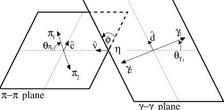
FIG. 2.: Choice of kinematical variables in the four-particle decay $\eta\rightarrow\pi\pi\gamma\gamma$.

                                             

                                             

FIG. 3.: Feynman diagrams of the process $\eta\rightarrow\pi^{+}\pi^{-}\gamma\gamma$. The numbers in the interaction blobs denote the order of the vertex in the momentum and quark mass expansion.

FIG. 4.: Feynman diagrams of the process $\eta\rightarrow\pi^{0}\pi^{0}\gamma\gamma$.

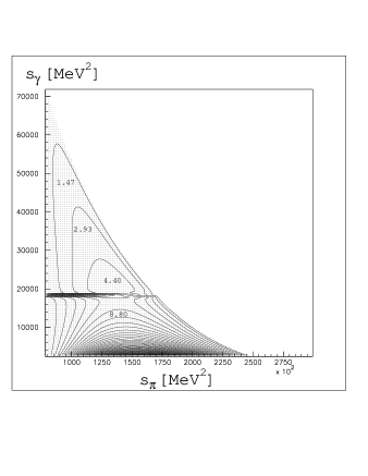
FIG. 5.: Dalitz contour plot for the full calculation in chiral perturbation theory. The distance between two contour lines corresponds to a difference of $1.47\times 10^{-17}\,{\mathrm{MeV}}^{-3}$ in the doubly differential decay rate ${\mathrm{d}}^{2}\Gamma/{\mathrm{d}}s_{\pi}{\mathrm{d}}s_{\gamma}$. The outermost contour line denotes the level ${\mathrm{d}}^{2}\Gamma/{\mathrm{d}}s_{\pi}{\mathrm{d}}s_{\gamma}=1.467\times 10^{-17}\,{\mathrm{MeV}}^{-3}.$ The dotted area is the physical region of the process. The dots in the $s_{\pi}$-$s_{\gamma}$ plane represent the points where the invariant amplitude was evaluated.

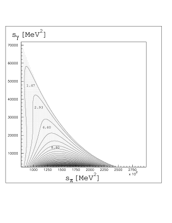
FIG. 6.: Dalitz contour plot for the chiral perturbation theory calculation without class 1 pole diagrams. The contour spacing is the same as in Fig. 5.

FIG. 7.: Diphoton energy spectrum ${\mathrm{d}}\Gamma/{\mathrm{d}}z\,\,\,(z=s_{\gamma}/m_{\eta}^{2})$ for the decay $\eta\rightarrow\pi^{+}\pi^{-}\gamma\gamma$. The dotted line is the full calculation, the dashed line is calculated without class 1 diagrams and the solid line is proportional to the phase space integral.

FIG. 8.: Partial decay rate $\Gamma(\eta\rightarrow\pi^{+}\pi^{-}\gamma\gamma)$ as a function of the energy cut $\delta m_{brems}$ around the bremsstrahlung singularity at $s_{\gamma}=0$.

FIG. 9.: Diphoton spectrum for the decay $\eta\rightarrow\pi^{0}\pi^{0}\gamma\gamma$ ($z=s_{\gamma}/m_{\eta}^{2}$). The long dash-dotted line is the prediction of chiral perturbation theory, the short dash-dotted line is the calculation in chiral perturbation theory, where the $\pi^{0}\pi^{0}\eta_{8}\eta_{8}$ interaction is set to $0$, and the dotted line is the prediction of chiral perturbation theory for $m_{u}=m_{d}$. The short dashed line is a calculation, where we determined the strength of the $\eta\pi^{0}\pi^{0}\pi^{0}$ interaction from the decay $\eta\rightarrow\pi^{0}\pi^{0}\pi^{0}$ and the $\eta\eta^{\prime}\pi^{0}\pi^{0}$ interaction from the decay $\eta^{\prime}\rightarrow\eta\pi^{0}\pi^{0}$. In the long dashed curve an additional $\eta_{8}\eta_{8}\pi^{0}\pi^{0}$ interaction is included. The solid line is proportional to the phase space integral.

FIG. 10.: Partial decay rate for the decay $\eta\rightarrow\pi^{0}\pi^{0}\gamma\gamma$ as a function of the energy cut $\delta m$ in $s_{\gamma}^{1/2}$ around $m_{\pi^{0}}$. The long dashed line is the calculation with the $\eta\pi^{0}\pi^{0}\pi^{0}$ and $\eta^{\prime}\eta\pi^{0}\pi^{0}$ vertices fixed by experiment. For the solid line we added a $\eta_{8}\eta_{8}\pi^{0}\pi^{0}$ interaction from chiral perturbation theory.

REFERENCES

• [1] V. S. Demidov and E. Shabalin, in The DA$\Phi$NE Physics Handbook, Vol. I (eds. L. Maiani, G. Pancheri and N. Paver), Servizio Documentazione dei Laboratori Nazionali di Frascati, Frascati (1992).
• [2] S. Weinberg, Physica 96A, 327 (1979).
• [3] J. Gasser and H. Leutwyler, Ann. Phys. (N.Y.) 158, 142 (1984); Nucl. Phys. B250, 465 (1985).
• [4] J. Gasser and H. Leutwyler, Nucl. Phys. B250, 539 (1985).
• [5] A. Pich, in Proc. of the Workshop on Rare Decays of Light Mesons, Gif-sur-Yvette (1990).
• [6] J. Wess and B. Zumino, Phys. Lett. 37B, 95 (1971).
• [7] E. Witten, Nucl. Phys. B223, 422 (1983).
• [8] J. Bijnens, Int. J. Mod. Phys. A8, 3045 (1993).
• [9] J. W. Bos, Y. C. Lin, H. H. Shih, Phys. Lett. B337, 152 (1994).
• [10] Paricle Data Group, Phys. Rev. D50 (1994).
• [11] L. R. Price and F. S. Crawford, Phys. Rev. Lett. 18, 1207 (1967).
• [12] C. Baltay et al., Phys. Rev. Lett. 19, 1498 (1967).
• [13] N. Cabibbo and A. Maksymowicz, Phys. Rev. B137 B438 (1965); erratum Phys. Rev. 168, 1926 (1968).
• [14] J. Bijnens, G. Ecker, and J. Gasser, in The DA$\Phi$NE Physics Handbook, Vol. I (eds. L. Maiani, G. Pancheri and N. Paver), Servizio Documentazione dei Laboratori Nazionali di Frascati, Frascati (1992).
• [15] F. J. Gilman and R. Kauffman, Phys. Rev. D36, 2761 (1987).
• [16] F. Halzen and A. D. Martin, Quarks and Leptons, (Wiley, New York, 1984), chapter 6.13.
• [17] H. Osborn and D. J. Wallace, Nucl. Phys. B20, 23 (1970).
• [18] B. Bagchi, A. Lahiri and S. Niyogi, Phys. Rev. D41, 2871 (1990).
• [19] V. V. Solovev and M. V. Terentev, Sov. J. Nucl. Phys. 16, 82 (1973).
Refer to caption