BUTP–95/2

Dispersive analysis of the decay $\eta\rightarrow 3\pi$
A. V. Anisovich

Academy of Sciences, Petersburg Nuclear Physics Institute

Gatchina, St. Petersburg, 188350 Russia

and

H. Leutwyler

Institut für theoretische Physik der Universität Bern

Sidlerstr. 5, CH-3012 Bern, Switzerland and

CERN, CH-1211 Geneva, Switzerland

January 1996

Abstract

We demonstrate that the decay $\eta\rightarrow 3\pi$ represents a sensitive probe for the breaking of chiral symmetry by the quark masses. The transition amplitude is proportional to the mass ratio $(m_{d}^{2}-m_{u}^{2})/(m_{s}^{2}-\hat{m}^{2})$. The factor of proportionality is calculated by means of dispersion relations, using chiral perturbation theory to determine the subtraction constants. The theoretical uncertainties in the result are shown to be remarkably small, so that $\eta$-decay may be used to accurately measure this ratio of quark masses.

 

Work supported in part by Schweizerischer Nationalfonds

1. Chiral perturbation theory. Since Bose statistics does not allow three pions to form a configuration where the total angular momentum and the total isospin both vanish, the decay $\eta\rightarrow 3\pi$ violates isospin symmetry. The transition amplitude contains terms proportional to the quark mass difference $m_{d}-m_{u}$ as well contributions $\propto e^{2}$, generated by the electromagnetic interaction. The latter are strongly suppressed by chiral symmetry – the transition is due almost exclusively to the isospin breaking part $\frac{1}{2}(m_{u}-m_{d})(\overline{\rule[4.19998pt]{3.99994pt}{0.0pt}}uu-\,\overline{\rule[6.49994pt]{3.99994pt}{0.0pt}}dd)$ of the QCD Hamiltonian [2]. Current algebra implies that the matrix element relevant for the transition $\eta\rightarrow\pi^{+}\pi^{-}\pi^{0}$ is given by

$$A=-\epsilon_{0}\,\frac{1}{F_{\pi}^{2}}\,(s-\mbox{$\frac{4}{3}$}\,M_{\pi}^{2})\;\;,\hskip 30.00005pt\epsilon_{0}\equiv\frac{\sqrt{3}}{\,4}\,\frac{(m_{d}-m_{u})}{(m_{s}-\hat{m})}\;\;,$$ (1)

where $F_{\pi}=92.4\,\mbox{MeV}$ is the pion decay constant, $s=(p_{\pi^{+}}+p_{\pi^{-}})^{2}$ and $\hat{m}$ denotes the mean mass of the $u$- and $d$-quarks, $\hat{m}\equiv\frac{1}{2}(m_{u}+m_{d})$.

The current algebra formula represents the leading contribution of the chiral perturbation series, which describes the decay amplitude as a sequence of terms involving increasing powers of momenta and quark masses. The corrections of first nonleading order (chiral perturbation theory to one loop) are also known [3]. If the amplitude is written in the form

$$A=-\frac{1}{Q^{2}}\,\frac{M_{K}^{2}}{M_{\pi}^{2}}\,\frac{M_{K}^{2}-M_{\pi}^{2}}{3\sqrt{3}F_{\pi}^{2}}\,M(s,t,u)\;\;,\;\;\;\frac{1}{Q^{2}}\equiv\frac{m_{d}^{2}\!-\!m_{u}^{2}}{m_{s}^{2}\!-\!\hat{m}^{2}}\;\;,$$ (2)

the one loop result for the dimensionless factor $M(s,t,u)$ exclusively involves measured quantities. It is of the form

$$M(s,t,u)=M_{0}(s)+(s\!-\!u)M_{1}(t)+(s\!-\!t)M_{1}(u)+M_{2}(t)+M_{2}(u)-\mbox{$\frac{2}{3}$}M_{2}(s)\;\;,$$ (3)

with $t=(p_{\pi^{-}}+p_{\pi^{0}})^{2}$, $u=(p_{\pi^{0}}+p_{\pi^{+}})^{2}$. The functions $M_{0}(s),M_{1}(s),M_{2}(s)$ represent contributions with isospin I = 0, 1, 2, respectively. They contain branch point singularities generated by the final state interaction in the S- and P-waves. The imaginary parts due to partial waves with angular momentum $\ell\geq 2$ only start showing up if the chiral perturbation series is evaluated to three or more loops. For this reason, the amplitude retains the structure (3) also at next-to-next-to-leading order. We stick to this approximation throughout the following, i.e. represent the amplitude in terms of the S- and P-waves and neglect the discontinuities from partial waves with $\ell\!\geq\!2$.

In current algebra approximation, only the I=0 component $M_{0}(s)$ is different from zero. According to eqs.(1) and (2), the leading term is given by $T(s)\equiv(3s-4M_{\pi}^{2})(M_{\eta}^{2}-M_{\pi}^{2})^{-1}$. The one loop calculation supplements this expression with corrections of first nonleading order and also gives rise to components with I=1,2. We denote the one loop approximation by $\;\overline{\rule[7.5pt]{8.00003pt}{0.0pt}}M_{0}(s),\;\overline{\rule[7.5pt]{8.00003pt}{0.0pt}}M_{1}(s),\;\overline{\rule[7.5pt]{8.00003pt}{0.0pt}}M_{2}(s)$. In the notation of ref.[3], the result reads

$$\;\overline{\rule[7.5pt]{8.00003pt}{0.0pt}}M_{0}(s) \!\!\!\!= \!\!\!\!T(s)+\Delta_{0}(s)\{1+\mbox{$\frac{2}{3}$}T(s)\}+\Delta_{2}(s)\{1-\mbox{$\frac{1}{3}$}T(s)\}+\Delta_{3}(s)+V(s)$$

$$\!\!\!\!+\mbox{$\frac{2}{3}$}\Delta_{\mbox{\tiny GMO}}T(s)+\mbox{$\frac{8}{3}$}M_{\pi}^{2}\,\{\Delta_{\mbox{\tiny F}}T(s)-\Delta_{\mbox{\tiny GMO}}\}(M_{\eta}^{2}-M_{\pi}^{2})^{-1}\;\;,$$

$$\;\overline{\rule[7.5pt]{8.00003pt}{0.0pt}}M_{1}(s) \!\!\!\!= \!\!\!\!\{\mbox{$\frac{3}{2}$}\Delta_{1}(s)-4sL_{3}F_{\pi}^{-2}\}(M_{\eta}^{2}-M_{\pi}^{2})^{-1}\;\;,$$

$$\;\overline{\rule[7.5pt]{8.00003pt}{0.0pt}}M_{2}(s) \!\!\!\!= \!\!\!\!\mbox{$\frac{1}{2}$}\Delta_{2}(s)\{3-T(s)\}\;\;.$$

The functions $\Delta_{0}(s),\ldots\,,\Delta_{3}(s)$ are generated by the final state interaction. They arise from one loop graphs, contain cuts along the real axis and are inversely proportional to $F_{\pi}^{2}$. The quantity $V(s)$ represents a subtraction term linear in $s$, which also originates in these graphs (for explicit expressions, see ref.[3]). The coefficients $\Delta_{\mbox{\tiny GMO}}$ and $\Delta_{\mbox{\tiny F}}$ are known low energy constants related to the masses and decay constants of the pseudoscalar octet. Finally, the term $L_{3}$ is an effective coupling constant of the chiral Lagrangian, whose value is known from $K_{\ell 4}$-decay [8].

The one loop formula shows that, up to and including first order corrections, the decay rate is inversely proportional to $Q^{4}$, with a known factor of proportionality. A measurement of the rate thus amounts to a measurement of the quark mass ratio $Q$. Apart from experimental uncertainties, the accuracy of the result for $Q$ is determined by the accuracy of the theoretical prediction for the factor $M(s,t,u)$. This motivates the present work.

In fig.1, the real part of the one loop amplitude is plotted along the line $s=u$ (dash-dotted). For small values of $s$, the curve very closely follows the current algebra formula (dashed) – there, the correction is small. The cusp at $s=4\,M_{\pi}^{2}$ arises from the final state interaction, which is dominated by the isospin zero S-wave. The singularity requires the amplitude to grow more strongly with $s$ than the current algebra result. At the maximal energy accessible in $\eta$-decay, $\sqrt{s}=M_{\eta}-M_{\pi}$, the correction amounts to $\frac{2}{3}$ of the leading term. This indicates that (a) the current algebra formula underestimates the rate by a substantial factor and (b) the first two terms of the chiral perturbation series represent a good approximation only at small values of $s$.

The reason why in part of the physical region, the corrections are unusually large is understood. Chiral symmetry implies that the pions are subject to an interaction with a strength determined by $F_{\pi}$. In the chiral limit the corresponding I=0 S-wave phase shift is given by $\delta_{0}^{0}=s/16\pi^{2}F_{\pi}^{2}$ and thus grows with the square of the center of mass energy. Accordingly, the corrections rapidly grow with the energy of the charged pion pair.

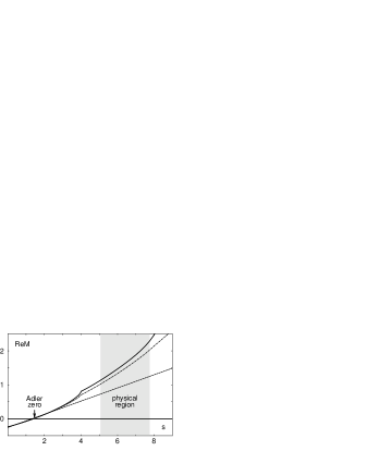
Figure 1: Real part of the amplitude along the line $s=u$. The dashed line is the current algebra prediction. The dash-dotted curve corresponds to the one loop approximation of chiral perturbation theory. The full line represents the result of the dispersive calculation described in the text.

2. Dispersion relations and sum rules. There is a well-known method which allows one to calculate the final state interaction effects, also if they are large: dispersion relations. Indeed, this method was applied to three-body decays long ago [9] and many papers concerning the decay $\eta\!\rightarrow\!3\pi$ have appeared in the meantime – they may be traced with refs.[10]–[13]. Crudely speaking, analyticity and unitarity determine the decay amplitude up to the subtraction constants. Chiral perturbation theory is needed only for these. The additional information contained in the one loop result merely reflects the fact that the chiral perturbation series obeys unitarity, order by order. In the following, we determine the absorptive part with unitarity and use dispersion relations to express the full amplitude in terms of the absorptive part and a set of subtraction constants. The latter are calculated by matching the dispersive and one loop representations at low energies. In principle, the same steps must be taken whenever unitarity is used to extend the range of validity of the effective theory – our analysis outlines the general procedure in the context of a nontrivial example. For a recent report on the marriage of chiral perturbation theory and dispersion relations, see ref.[14].

We first set up the dispersion relations obeyed by the one loop amplitude. The functions $\;\overline{\rule[7.5pt]{8.00003pt}{0.0pt}}M_{0}(s),\;\overline{\rule[7.5pt]{8.00003pt}{0.0pt}}M_{1}(s),\;\overline{\rule[7.5pt]{8.00003pt}{0.0pt}}M_{2}(s)$ are analytic except for a cut along the real axis. For $s\!\rightarrow\!\infty$, $\;\overline{\rule[7.5pt]{8.00003pt}{0.0pt}}M_{0}(s)$ and $\;\overline{\rule[7.5pt]{8.00003pt}{0.0pt}}M_{2}(s)$ grow like $s^{2}\,\mbox{log}s$, while $\;\overline{\rule[7.5pt]{8.00003pt}{0.0pt}}M_{1}(s)$ is of order $s\,\mbox{log}s$. Accordingly, three subtractions are needed for $\;\overline{\rule[7.5pt]{8.00003pt}{0.0pt}}M_{0}(s),\;\overline{\rule[7.5pt]{8.00003pt}{0.0pt}}M_{2}(s)$ and two for $\;\overline{\rule[7.5pt]{8.00003pt}{0.0pt}}M_{1}(s)$,

$$\;\overline{\rule[7.5pt]{8.00003pt}{0.0pt}}M_{0}(s) \!\!\!\!= \!\!\!\!a_{0}+b_{0}s+c_{0}s^{2}+\frac{s^{3}}{\pi}\!\int_{4M_{\pi}^{2}}^{\infty}\frac{ds^{\prime}}{s^{\prime\,3}}\frac{\mbox{Im}\;\overline{\rule[7.5pt]{8.00003pt}{0.0pt}}M_{0}(s^{\prime})}{s^{\prime}-s-i\epsilon}\;\;,$$

$$\;\overline{\rule[7.5pt]{8.00003pt}{0.0pt}}M_{1}(s) \!\!\!\!= \!\!\!\!a_{1}+b_{1}s+\frac{s^{2}}{\pi}\!\int_{4M_{\pi}^{2}}^{\infty}\frac{ds^{\prime}}{s^{\prime\,2}}\frac{\mbox{Im}\;\overline{\rule[7.5pt]{8.00003pt}{0.0pt}}M_{1}(s^{\prime})}{s^{\prime}-s-i\epsilon}\;\;,$$ (4)

$$\;\overline{\rule[7.5pt]{8.00003pt}{0.0pt}}M_{2}(s) \!\!\!\!= \!\!\!\!a_{2}+b_{2}s+c_{2}s^{2}+\frac{s^{3}}{\pi}\!\int_{4M_{\pi}^{2}}^{\infty}\frac{ds^{\prime}}{s^{\prime\,3}}\frac{\mbox{Im}\;\overline{\rule[7.5pt]{8.00003pt}{0.0pt}}M_{2}(s^{\prime})}{s^{\prime}-s-i\epsilon}\;\;.$$

Inserting this representation in eq.(3), the one loop amplitude takes the form $M(s,t,u)=P(s,t,u)+D(s,t,u)$, where the polynomial $P(s,t,u)$ contains the contributions from the subtraction constants $a_{0},\ldots,c_{2}$ while $D(s,t,u)$ collects the dispersion integrals. On kinematic grounds, the polynomial only involves four independent terms, which may be written in the form $P(s,t,u)=a+b\,s+c\,s^{2}-d\,(s^{2}+2\,t\,u)$: Only four combinations of the eight subtraction constants $a_{0},\ldots,c_{2}$ are of physical significance.

The dispersive representation of the one loop amplitude thus appears to involve four subtraction constants. In fact, however, the constant $c$ is determined by the imaginary parts through a sum rule, for the following reason. The amplitudes $\;\overline{\rule[7.5pt]{8.00003pt}{0.0pt}}M_{0}(s)$ and $\;\overline{\rule[7.5pt]{8.00003pt}{0.0pt}}M_{2}(s)$ individually grow like $s^{2}\,\mbox{log}s$ for $s\!\rightarrow\!\infty$, but the combination $\;\overline{\rule[7.5pt]{8.00003pt}{0.0pt}}M_{0}(s)+\frac{4}{3}\;\overline{\rule[7.5pt]{8.00003pt}{0.0pt}}M_{2}(s)$ only diverges in proportion to $s\,\mbox{log}s$. For the above representation to reproduce this behaviour at large values of $s$, the term $\propto\!s^{2}$ arising from the dispersion integrals must be compensated by the one from the subtraction polynomials, i.e.

$$c=c_{0}+\mbox{$\frac{4}{3}$}c_{2}=\frac{1}{\pi}\int_{4M_{\pi}^{2}}^{\infty}\frac{ds^{\prime}}{s^{\prime\,3}}\{\mbox{Im}\;\overline{\rule[7.5pt]{8.00003pt}{0.0pt}}M_{0}(s^{\prime})+\mbox{$\frac{4}{3}$}\,\mbox{Im}\;\overline{\rule[7.5pt]{8.00003pt}{0.0pt}}M_{2}(s^{\prime})\}\;\;.$$ (5)

The terms of order $s^{2}\,\mbox{log}s$ also cancel in the combination $s\,\;\overline{\rule[7.5pt]{8.00003pt}{0.0pt}}M_{1}(s)+\;\overline{\rule[7.5pt]{8.00003pt}{0.0pt}}M_{2}(s)$, but this function does not obey a twice subtracted dispersion relation, because the term $\propto L_{3}$ gives rise to a contribution which grows like $s^{2}$. Hence $d$ is related to the effective coupling constant $L_{3}$,

$$d=b_{1}+c_{2}=-\frac{(4L_{3}-1/64\pi^{2})}{F_{\pi}^{2}(M_{\eta}^{2}-M_{\pi}^{2})}+\frac{1}{\pi}\int_{4M_{\pi}^{2}}^{\infty}\frac{ds^{\prime}}{s^{\prime\,3}}\{s^{\prime}\,\mbox{Im}\;\overline{\rule[7.5pt]{8.00003pt}{0.0pt}}M_{1}(s^{\prime})+\mbox{Im}\;\overline{\rule[7.5pt]{8.00003pt}{0.0pt}}M_{2}(s^{\prime})\}\;\;.$$ (6)

This shows that the one loop amplitude is fully determined by its imaginary parts and by the three constants $a,b$ and $L_{3}$. The dispersive representation explicitly expresses the fact that an analytic function is uniquely determined by its singularities: While the functions $\mbox{Im}\;\overline{\rule[7.5pt]{8.00003pt}{0.0pt}}M_{\mbox{\scriptsize I}}(s)$ describe those associated with the branch cut along the real axis, the subtraction constants account for the singularities at infinity.

3. Unitarity. In one loop approximation, the amplitude obeys unitarity only modulo contributions of order $p^{6}$. The corresponding expressions for the discontinuities across the branch cut only hold to leading order of the chiral expansion. The unitarity condition may be solved more accurately, using an approximation which holds up to and including two loops of chiral perturbation theory. The approximation accounts for two-body collisions, but disregards multiparticle interactions. In the case of elastic scattering, the approximation is well-known and is referred to as elastic unitarity. The extension of this notion to three-body decays is not trivial, however: Some of the early papers contain erroneous prescriptions. A coherent framework is obtained with analytic continuation in the mass of the $\eta$. One first considers the scattering amplitude $\pi\eta\!\rightarrow\!\pi\pi$ for a value of the strange quark mass for which $M_{\eta}\!<\!3M_{\pi}$, such that the decay is kinematically forbidden. Elastic unitarity then represents a consistent approximation scheme. In this approximation, only two-pion intermediate states are taken into account, such that the imaginary part of the scattering amplitude coincides with the discontinuity across the two-pion cut and is determined by the phase shifts of $\pi\pi$ scattering. Denoting the discontinuity of the function $M_{\mbox{\scriptsize I}}(s)$ by $\mbox{disc}\,M_{\mbox{\scriptsize I}}(s)\!\equiv\!\{M_{\mbox{\scriptsize I}}(s+i\epsilon)-M_{\mbox{\scriptsize I}}(s-i\epsilon)\}/2i$, the elastic unitarity conditions read

$$\mbox{disc}\,M_{\mbox{\scriptsize I}}(s)=\sin\delta_{\mbox{\scriptsize I}}(s)\,e^{-i\delta_{\mbox{\tiny I}}(s)}\{M_{\mbox{\scriptsize I}}(s)+\hat{M}_{\mbox{\scriptsize I}}(s)\}\;\;.$$ (7)

The first term in the curly brackets accounts for repeated collisions in the $s$-channel, while the second arises from two-particle final state interactions in the $t$- and $u$-channels and involves angular averages of the type

$$\!\!\langle z^{n}M_{\mbox{\scriptsize I}}\,\rangle(s)\equiv\mbox{$\frac{1}{2}$}\int_{-1}^{+1}\!dzz^{n}M_{\mbox{\scriptsize I}}\,(\mbox{$\frac{3}{2}$}s_{0}-\mbox{$\frac{1}{2}$}s+\mbox{$\frac{1}{2}$}\kappa z)\;\;,$$

$$\!\!\kappa\equiv\left\{(1-4M_{\pi}^{2}/s)\{(M_{\eta}+M_{\pi})^{2}-s\}\{(M_{\eta}-M_{\pi})^{2}-s\}\right\}^{\frac{1}{2}}\;\;,$$

with $s_{0}\!\equiv\!\frac{1}{3}M_{\eta}^{2}+M_{\pi}^{2}$. In this notation, the explicit expression for the discontinuity due to two-body collisions in the crossed channels reads

$$\hat{M}_{0} \!\!= \!\!\mbox{$\frac{2}{3}$}\langle M_{0}\rangle+\mbox{$\frac{20}{9}$}\langle M_{2}\rangle+2(s-s_{0})\langle M_{1}\rangle+\mbox{$\frac{2}{3}$}\kappa\,\langle zM_{1}\rangle$$

$$\hat{M}_{1} \!\!= \!\!\kappa^{-1}\,\{3\langle zM_{0}\rangle-5\langle zM_{2}\rangle+\mbox{$\frac{9}{2}$}(s-s_{0})\langle zM_{1}\rangle+\mbox{$\frac{3}{2}$}\kappa\,\langle z^{2}M_{1}\rangle\}$$

$$\hat{M}_{2} \!\!= \!\!\langle M_{0}\rangle+\mbox{$\frac{1}{3}$}\langle M_{2}\rangle-\mbox{$\frac{3}{2}$}(s-s_{0})\langle M_{1}\rangle-\mbox{$\frac{1}{2}$}\kappa\,\langle zM_{1}\rangle\;\;.$$

In contrast to the imaginary parts, the discontinuities are analytic in $M_{\eta}$, so that the above relations may be continued to the physical value of the mass. While the imaginary parts are real by definition, the two particle discontinuities obtained through analytic continuation are complex. In the unitarity relation for the decay amplitude, these contributions arise from the disconnected part of the $T$-matrix, describing two-particle collisions with the third pion as a spectator. The imaginary part of the amplitude necessarily also receives contributions from the connected part. In the above approximation, these arise from successive collisions among two different pairs of pions. Note also that the dispersion integrals extend beyond the physical region of the decay, where $\kappa$ may develop an imaginary part. The integration over $z$ must then be deformed into the complex plane, in such a way that the path avoids the branch cut (for details, see ref.[12]).

The conditions (7) specify the approximate form of unitarity used in our analysis. We briefly comment on the three phase shifts $\delta_{0}(s),\delta_{1}(s),\delta_{2}(s)$ which occur in these conditions and which represent an important input of our calculation. Chiral perturbation theory yields remarkably sharp predictions near threshold. Together with the experimental information available at higher energies, the Roy equations then determine their behaviour up to $K\,\overline{\rule[7.5pt]{6.99997pt}{0.0pt}}K$ threshold, to within small uncertainties [15]. The function $\delta_{0}(s)$ slowly passes through $\frac{1}{2}\pi$ at $\sqrt{s}=850-900$ MeV and continues rising beyond this point. In the context of our calculation, the behaviour at higher energies does not play a crucial role. We use a parametrization where $\delta_{0}(s)$ tends to $\pi$ for $s\rightarrow\infty$, so that the discontinuity, which is proportional to $\sin\delta_{0}(s)$, tends to zero. A similar representation of the high energy behaviour is also used for the P-wave, where the phase shift rapidly passes through $\frac{1}{2}\pi$ at $s=M_{\rho}^{2}$. The exotic partial wave with I=2, on the other hand, describes a repulsive interaction and does not exhibit resonance behaviour. We use a parametrization where the function $\delta_{2}(s)$ asymptotically tends to zero.

4. Ambiguities in the solution of the dispersion relations. If the phase shifts are known, the unitarity conditions determine the discontinuity across the branch cut in terms of the amplitude itself. Analyticity then implies that the functions $M_{0}(s),M_{1}(s)$ and $M_{2}(s)$ obey dispersion relations analogous to eq.(S0.Ex5),

$$M_{\mbox{\scriptsize I}}(s)=P_{\mbox{\scriptsize I}}(s)+\frac{1}{\pi}\int_{4M_{\pi}^{2}}^{\infty}\!ds^{\prime}\,\frac{\sin\delta_{\mbox{\scriptsize I}}(s^{\prime})e^{-i\delta_{\mbox{\tiny I}}(s^{\prime})}}{s^{\prime}-s-i\epsilon}\{M_{\mbox{\scriptsize I}}(s^{\prime})+\hat{M}_{\mbox{\scriptsize I}}(s^{\prime})\}\;\;.$$ (8)

For simplicity, we assume that the phase shifts rapidly reach their asymptotic values, so that the dispersion integrals converge without subtractions, but this is not essential – we might just as well write the integrals in subtracted form, absorbing the difference in the polynomials $P_{\mbox{\scriptsize I}}(s)$.

It is crucial that the dispersion relations used uniquely determine the amplitude. In fact for the above relations this is not the case: The corresponding homogeneous equations – obtained by dropping the polynomials $P_{\mbox{\scriptsize I}}(s)$ – possess nontrivial solutions. In its simplest form, the problem shows up if the contributions to the discontinuity from the angular averages over the crossed channels are dropped. Unitarity then reduces to three independent constraints of the form $\mbox{disc}M_{\mbox{\scriptsize I}}\!=\!\sin\delta_{\mbox{\scriptsize I}}\,e^{-i\delta_{\mbox{\tiny I}}}M_{\mbox{\scriptsize I}}$, or, equivalently, $M_{\mbox{\scriptsize I}}(s+i\epsilon)\!=\!e^{2i\delta_{\mbox{\tiny I}}}M_{\mbox{\scriptsize I}}(s-i\epsilon)$. This condition is well-known from the dispersive analysis of form factors and can be solved explicitly: The Omnès function, defined by

$$\Omega_{\mbox{\scriptsize I}}(s)=\exp\left\{\frac{s}{\pi}\int_{4M_{\pi}^{2}}^{\infty}\!\frac{ds^{\prime}}{s^{\prime}}\frac{\delta_{\mbox{\scriptsize I}}(s^{\prime})}{(s^{\prime}-s-i\epsilon)}\right\}\;\;,$$

obeys $\Omega_{\mbox{\scriptsize I}}(s+i\epsilon)\!=\!e^{2i\delta_{\mbox{\tiny I}}}\,\Omega_{\mbox{\scriptsize I}}(s-i\epsilon)$, so that the ratio $m_{\mbox{\scriptsize I}}(s)\!=\!M_{\mbox{\scriptsize I}}(s)/\Omega_{\mbox{\scriptsize I}}(s)$ is continuous across the cut. Since $\Omega_{\mbox{\scriptsize I}}(s)$ does not have any zeros, $m_{\mbox{\scriptsize I}}(s)$ is an entire function. In view of the asymptotic behaviour of the phase shifts specified above, $\Omega_{0}(s),\Omega_{1}(s)$ tend to zero in inverse proportion to $s$, while $\Omega_{2}(s)$ approaches a constant. Assuming that $M_{\mbox{\scriptsize I}}(s)$ does not grow faster than a power of $s$, the same then also holds for $m_{\mbox{\scriptsize I}}(s)$. Being entire, $m_{0}(s),m_{1}(s)$ and $m_{2}(s)$ thus represent polynomials: The general solution of the simplified unitarity conditions is of the form $M_{\mbox{\scriptsize I}}(s)\!=\!m_{\mbox{\scriptsize I}}(s)\,\Omega_{\mbox{\scriptsize I}}(s)$, where $m_{\mbox{\scriptsize I}}(s)$ is a polynomial. The ambiguity mentioned above arises because the Omnès factors belonging to the partial waves with I=0,1 tend to zero for $s\rightarrow\infty$. The dispersion relation for $M_{0}(s)$, e.g. implies $M_{0}(s)\rightarrow P_{0}(s)$. If $P_{0}(s)$ is a polynomial of degree $n$, $m_{0}(s)$ is of degee $n+1$. Hence the above dispersion relation for $M_{0}(s)$ admits a one parameter family of solutions. The same is true of $M_{1}(s)$, while the solution of the dispersion relation for $M_{2}(s)$ is unique.

The same problem also occurs if the angular averages are not discarded. The preceding discussion points the way towards a solution of the problem: It suffices to replace the above integral equations with the dispersion relations obeyed by the functions $m_{\mbox{\scriptsize I}}(s)\equiv M_{\mbox{\scriptsize I}}(s)/\Omega_{\mbox{\scriptsize I}}(s)$. Since the corresponding discontinuities are given by

$$\frac{M_{\mbox{\scriptsize I}}(s+i\epsilon)}{\Omega_{\mbox{\scriptsize I}}(s+i\epsilon)}-\frac{M_{\mbox{\scriptsize I}}(s-i\epsilon)}{\Omega_{\mbox{\scriptsize I}}(s-i\epsilon)}=\frac{M_{\mbox{\scriptsize I}}(s+i\epsilon)e^{\!-i\delta_{\mbox{\tiny I}}}\!-\!M_{\mbox{\scriptsize I}}(s-i\epsilon)e^{i\delta_{\mbox{\tiny I}}}}{|\Omega_{\mbox{\scriptsize I}}|}=2i\,\frac{\sin\delta_{\mbox{\scriptsize I}}\hat{M}_{\mbox{\scriptsize I}}}{|\Omega_{\mbox{\scriptsize I}}|}\;\;,$$

the dispersion relations take the form

$$M_{\mbox{\scriptsize I}}(s)=\Omega_{\mbox{\scriptsize I}}(s)\left\{\tilde{P}_{\mbox{\scriptsize I}}(s)+\frac{1}{\pi}\!\int_{4M_{\pi}^{2}}^{\infty}\!ds^{\prime}\,\frac{\sin\delta_{\mbox{\scriptsize I}}(s^{\prime})\,\hat{M}_{\mbox{\scriptsize I}}(s^{\prime})}{|\Omega_{\mbox{\scriptsize I}}(s^{\prime})|\,(s^{\prime}-s-i\epsilon)}\right\}\;\;.$$ (9)

In the simplified situation considered above, where the angular averages $\hat{M}_{\mbox{\scriptsize I}}(s)$ are discarded, this form of the dispersion relations indeed unambiguously fixes the solution in terms of the polynomials $\tilde{P}_{\mbox{\scriptsize I}}(s)$. Our numerical results indicate that the same is true also for the full set of coupled integral equations, but we do not have an analytic proof of this statement.

In the present context, the asymptotic behaviour of the phase shifts is an academic issue. The fact that the solution of eq.(8) is unique if all of the phase shifts tend to zero, but becomes ambiguous if some of them tend to $\pi$, shows that this form of the dispersive framework is deficient. As an illustration, we return to the simplified problem and discuss the change in the function $M_{0}(s)$ which results if the high energy behaviour of the phase shift $\delta_{0}(s)$ is modified. Suppose that $\delta_{0}(s)$ is taken to rapidly drop to zero at some large value $s_{0}$, such that the corresponding Omnès function differs from the original one by the factor $1-s/s_{0}$. If the dispersion relations are written in the form (9), the solution merely picks up this factor and thus only receives a small correction at low energies. With eq.(8), however, the modification generates a qualitative change, as it selects a unique member from a one parameter family of solutions – the result cannot be trusted, because it is sensitive to physically irrelevant modifications of the input.

5. Subtractions. The high energy behaviour of the amplitude is the same as in the case of elastic scattering and is dominated by Pomeron exchange (since the amplitude $\pi\eta\rightarrow\pi\pi$ violates isospin symmetry, the coupling to the Pomeron is suppressed by a factor of $m_{d}\!-\!m_{u}$, but this holds for the entire amplitude). Comparison with $\pi\pi$-scattering indicates that, in principle, the dispersive representation of the three functions $M_{0}(s),M_{1}(s),M_{2}(s)$ should require only two subtractions. The chiral perturbation series yields an oversubtracted representation: The number of subtractions grows with the order at which the series is evaluated.

If only two subtractions are made, the contributions from the region above $K\,\overline{\rule[7.5pt]{6.99997pt}{0.0pt}}K$-threshold are quite important and need to be analyzed in detail (compare e.g. ref.[16], where the scalar form factors are studied by using unitarity also for the quasi-elastic transition $\pi\pi\!\rightarrow\!K\,\overline{\rule[7.5pt]{6.99997pt}{0.0pt}}K$). The uncertainties associated with the high energy part of the dispersion integrals do not limit the accuracy of the measurement of $Q$, however. One may use more than the minimal number of subtractions and determine the extra subtraction constants with the observed Dalitz plot distribution. With sufficiently many subtractions, the contributions from the high energy region become negligibly small. In principle, a measurement of $Q$ requires theoretical input only for the overall normalization, while the remaining subtraction constants, which specify the dependence of the amplitude on $s,t,u$, may be determined experimentally.

We do not invoke the observed Dalitz plot distribution, but use chiral perturbation theory to determine the subtraction constants. The number of subtractions is chosen such that $M(s,t,u)$ grows at most linearly in all directions $s,t,u\!\rightarrow\!\infty$: $M_{0}(s)\!=\!O(s),M_{1}(s)\!=\!O(1),M_{2}(s)\!=\!O(s)$. In view of the Omnès factors, this implies that the subtraction polynomials are of the form $\tilde{P}_{0}(s)\!=\!\alpha_{0}\!+\!\beta_{0}s\!+\!\gamma_{0}s^{2},\tilde{P}_{1}(s)\!=\!\alpha_{1}\!+\!\beta_{1}s,\tilde{P}_{2}(s)\!=\!\alpha_{2}\!+\!\beta_{2}s$ and thus involve altogether seven subtraction constants. As it is the case with the one loop amplitude, the decomposition into the three isospin components $M_{0}(s),M_{1}(s),M_{2}(s)$ is not unique. Since the transformation $M_{1}(s)\rightarrow M_{1}(s)+k_{1}$, $M_{2}(s)\rightarrow M_{2}(s)+k_{2}+k_{3}\,s$ preserves the asymptotic behaviour and can be absorbed in $M_{0}(s)$, only four of the seven subtraction constants are of physical significance. Without loss of generality we exploit this freedom in the isospin decomposition and set $\alpha_{1}\!=\!\alpha_{2}\!=\!\beta_{2}\!=\!0$. The dispersion relations then take the form

$$M_{0}(s) \!\!\!\!= \!\!\!\!\Omega_{0}(s)\left\{\alpha_{0}+\beta_{0}s+\gamma_{0}s^{2}+\frac{s^{2}}{\pi}\!\int_{4M_{\pi}^{2}}^{\infty}\!\frac{ds^{\prime}}{s^{\prime\,2}}\frac{\sin\delta_{0}(s^{\prime})\,\hat{M}_{0}(s^{\prime})}{|\Omega_{0}(s^{\prime})|\,(s^{\prime}-s-i\epsilon)}\right\}$$

$$M_{1}(s) \!\!\!\!= \!\!\!\!\Omega_{1}(s)\left\{\beta_{1}s+\frac{s}{\pi}\!\int_{4M_{\pi}^{2}}^{\infty}\!\frac{ds^{\prime}}{s^{\prime}}\frac{\sin\delta_{1}(s^{\prime})\,\hat{M}_{1}(s^{\prime})}{|\Omega_{1}(s^{\prime})|\,(s^{\prime}-s-i\epsilon)}\right\}$$ (10)

$$M_{2}(s) \!\!\!\!= \!\!\!\!\Omega_{2}(s)\frac{s^{2}}{\pi}\!\int_{4M_{\pi}^{2}}^{\infty}\!\frac{ds^{\prime}}{s^{\prime\,2}}\frac{\sin\delta_{2}(s^{\prime})\,\hat{M}_{2}(s^{\prime})}{|\Omega_{2}(s^{\prime})|\,(s^{\prime}-s-i\epsilon)}\;\;.$$

The four subtraction constants $\alpha_{0},\beta_{0},\gamma_{0},\beta_{1}$ play the same role as the terms $a,b,c,d$ occurring in the one loop result.

The constants $\alpha_{0},\beta_{0}$ already appear in the current algebra approximation, which corresponds to $\alpha_{0}+\beta_{0}\,s\!=\!(3s-4M_{\pi}^{2})/(M_{\eta}^{2}-M_{\pi}^{2})$. At leading order, the amplitude thus vanishes at $s\!=\!\frac{4}{3}M_{\pi}^{2}$, a feature which is beautifully confirmed by the observed Dalitz plot distribution. The phenomenon is a consequence of SU(2)${}_{\scriptscriptstyle R}\times$SU(2)_L-symmetry and does not rely on the expansion in powers of $m_{s}$, which is generating the main uncertainties in the chiral representation: In the limit $m_{u}\!=\!m_{d}\!=\!0$, where the pions are massless, the decay amplitude contains two Adler zeros, one at $p_{\pi^{+}}\!\!=\!0\,(s\!=\!u\!=\!0)$, the other at $p_{\pi^{-}}\!\!=\!0\,(s\!=\!t\!=\!0)$. The perturbations generated by $m_{u},m_{d}$ produce a small imaginary part, but the line $\mbox{Re}M(s,t,u)\!=\!0$ still passes through the vicinity of the above two points. The figure shows that along the line $s\!=\!u$, the one loop corrections shift the Adler zero from $1.33\,M_{\pi}^{2}$ to $s_{A}\!=\!1.41\,M_{\pi}^{2}$. The position of the zero is related to the value of the constant $\alpha_{0}$, while $\beta_{0}$ determines the slope of the curve there. The figure also shows that the corrections of order $m_{s}$ barely modify the latter: The slope of the one loop amplitude differs from the current algebra result, $\beta_{0}=3/(M_{\eta}^{2}-M_{\pi}^{2})$, by less than a percent. We therefore assume chiral perturbation theory to be reliable in the vicinity of the Adler zero and determine the subtraction constants $\alpha_{0}$ and $\beta_{0}$ by matching the dispersive representation of the amplitude with the one loop representation there. More specifically, we require that the first two terms in the Taylor series

$$M(s,3s_{0}-2s,s)=M_{A}+(s-s_{A})S_{A}+O\{(s-s_{A})^{2}\}$$

agree with those of the one loop amplitude, where

$$M_{A}=-0.0041\,i\;\;,\;\;\;\;S_{A}=(0.1957-0.0519\,i)\,M_{\pi}^{-2}\;\;.$$

Concerning the value of $\alpha_{0}$, this procedure is safe, because $\alpha_{0}$ is protected by the low energy theorem mentioned above. The slope, on the other hand, is not controlled by SU(2)${}_{\scriptscriptstyle R}\times$SU(2)_L. The one loop result does account for the corrections of order $m_{s}$, but disregards higher order contributions. According to a general rule of thumb, first order SU(3) breaking effects are typically of order $25\%$ while second order contributions are of the order of the square of this. It so happens that in the case of the slope, the various first order corrections nearly cancel one another. The second order effects are discussed in some detail in ref.[17], on the basis of the large $N_{c}$ expansion. In particular, it is shown there that the one loop result fully accounts for $\eta\eta^{\prime}$ mixing [18], except for a factor of $\cos\theta_{\eta\eta^{\prime}}\!\simeq\!0.93$. This represents a second order correction of typical size, consistent with the rule of thumb.

In the convention adopted above, the term $\beta_{1}$ determines the slope of $M_{1}(s)$. More generally, $\beta_{1}$ is related to the convention independent quantity

$$M^{\prime}_{1}(0)+\mbox{$\frac{1}{2}$}M^{\prime\prime}_{2}(0)=\beta_{1}+\frac{1}{\pi}\!\int_{4M_{\pi}^{2}}^{\infty}\!ds^{\prime}\left\{\frac{\sin\delta_{1}(s^{\prime})\hat{M}_{1}(s^{\prime})}{s^{\prime\,2}|\Omega_{1}(s^{\prime})|}+\frac{\sin\delta_{2}(s^{\prime})\hat{M}_{2}(s^{\prime})}{s^{\prime\,3}|\Omega_{2}(s^{\prime})|}\right\}\;\;.$$ (11)

In one loop approximation, the lhs coincides with $b_{1}+c_{2}$. The low energy theorem (6) thus relates $\beta_{1}$ to the coupling constant $L_{3}$, whose value is known rather accurately from $K_{\ell_{4}}$ decay, $L_{3}\!=\!(-3.5\pm 1.1)\cdot 10^{-3}$ [8].

Both for the dispersive representation and for the one loop approximation, the quantity $M^{\prime}_{1}(0)+\frac{1}{2}M^{\prime\prime}_{2}(0)$ receives two contributions: one from an integral over the discontinuities of the amplitude, which accounts for the effects generated by the low lying states, and one from a subtraction term $\{\beta_{1}\leftrightarrow-(4L_{3}-1/64\pi^{2})/F_{\pi}^{2}(M_{\eta}^{2}-M_{\pi}^{2})\}$, which incorporates all other singularities, including those at infiniy. The main difference between the two representations is that the integral in eq.(11) exclusively accounts for the $\pi\pi$ discontinuities, while the one in eq.(6) includes the singularities generated by $K\,\overline{\rule[7.5pt]{6.99997pt}{0.0pt}}K,\pi\eta$ and $\eta\eta$ intermediate states, albeit only to one loop. One readily checks that the integrals over the elastic region $4M_{\pi}^{2}\!<\!s\!<\!(M_{\eta}+M_{\pi})^{2}$ only differ by terms of order $p^{2}$, which are beyond the accuracy of the one loop prediction. This is an immediate consequence of the fact that chiral perturbation theory is consistent with unitarity. In the elastic region, the dispersive calculation yields a more accurate representation of the discontinuities than the one loop approximation. Accordingly, we use this approximation only to estimate the remainder. The one loop result shows that the contributions from $\pi\eta$ intermediate states are proportional to $M_{\pi}^{2}$ and therefore tiny – inelastic channels generate significant effects only for $4M_{K}^{2}\!<\!s\!<\!\infty$. The entire contribution from this interval to the integral in eq.(6) amounts to a shift in $\beta_{1}$ of $+1.7\,\mbox{GeV}^{-4}$, too small to stick out from the uncertainties in the term from $L_{3}$. We conclude that $\beta_{1}$ is dominated by this term,

$$\beta_{1}\simeq-\,\frac{\;4L_{3}-1/64\pi^{2}}{F_{\pi}^{2}\,(M_{\eta}^{2}-M_{\pi}^{2})}=6.5\pm 1.8\,\mbox{GeV}^{-4}\;\;.$$

and take the above shift as an estimate for the uncertainties associated with the inelastic channels.

The constant $\gamma_{0}$ is related to the convention independent combination $M_{0}^{\prime\prime}(0)+\frac{4}{3}M_{2}^{\prime\prime}(0)$ of Taylor coefficients and may be evaluated in the same manner. In particular, one may check that the elastic contributions to the relevant integrals coincide within the accuracy of the one loop representation also in this case. The only difference is that the low energy theorem (5) does not contain a term analogous to $L_{3}$, so that the arguments outlined in the preceding paragraph now imply $\gamma_{0}\simeq 0$. The uncertainties to be attached to this result may again be estimated with the contribution from the interval $4M_{K}^{2}\!<\!s\!<\!\infty$ to the integral over the imaginary part of the one loop amplitude, which amounts to a shift in the value of $\gamma_{0}$ by $+8.6\,\mbox{GeV}^{-4}$. The net effect of the uncertainties in the subtraction constants $\beta_{1},\gamma_{0}$ is small. At the center of the Dalitz plot, the above shifts due to inelastic discontinuities increase the amplitude by about $5\,\%$. The order of magnitude is comparable with the shift in $\beta_{0}$ due to $\eta\eta^{\prime}$ mixing, which acts in the opposite direction.

6. Iterative construction of the solution. Since the system is linear, the dependence of the solution on the subtraction constants $\alpha_{0},\beta_{0},\gamma_{0}$ and $\beta_{1}$ is of the form $M_{\mbox{\scriptsize I}}(s)=\alpha_{0}\,f_{\hskip 0.41998pt\mbox{\scriptsize I}}(s)+\beta_{0}\,g_{\hskip 0.41998pt\mbox{\scriptsize I}}(s)+\gamma_{0}\,h_{\hskip 0.41998pt\mbox{\scriptsize I}}(s)+\beta_{1}\,k_{\hskip 0.41998pt\mbox{\scriptsize I}}(s)$. The coefficients $f_{0}(s),f_{1}(s),f_{2}(s)$ represent the solution for $\alpha_{0}\!=\!1,\beta_{0}\!=\!\gamma_{0}\!=\!\beta_{1}\!=\!0$ and similarly for the other terms. The solutions may be obtained iteratively, starting e.g. with $M_{\mbox{\scriptsize I}}(s)\!=\!0$. Once the iteration has been performed for the four fundamental solutions defined above, the values of $\alpha_{0},\beta_{0}$ for which the Adler condition is met are readily worked out: Denote the total amplitudes which corresponds to the four sets of isospin coefficients by $f(s,t,u),g(s,t,u),h(s,t,u),k(s,t,u)$, restrict these to the line $s\!=\!u$ and calculate the values as well as the first derivatives at the point $s_{A}\!=\!1.41\,M_{\pi}^{2}$. The requirement that the sum $M=\alpha_{0}\,f+\beta_{0}\,g+\gamma_{0}\,h+\beta_{1}k$ agrees with the one loop amplitude there, both in value and slope, amounts to two linear equations for $\alpha_{0}$ and $\beta_{0}$.

The numerical results obtained with the above dispersive machinery are illustrated in fig.1: The solid line shows the real part of the amplitude along the line $s\!=\!u$, which connects one of the Adler zeros with the center of the Dalitz plot. As can be seen from this figure, the corrections to the one loop result are rather modest. The calculation confirms the crude estimates given in ref.[3]. The error bars to be attached to the dispersive evaluation are remarkably small. They are dominated by the uncertainties in the low energy theorems used to determine the subtraction constants. A more detailed account of our numerical results is in preparation [19].

We are indebted to V. V. Anisovich, Hans Bebie, Jürg Gasser and Peter Minkowski for useful comments and generous help with computer ethonography and to Joachim Kambor, Christian Wiesendanger and Daniel Wyler for keeping us informed about closely related work [13].

References

- [1]
-
[2]
D. G. Sutherland, Phys. Lett. 23 (1966) 384;
J. S. Bell and D. G Sutherland, Nucl. Phys. B4 (1968) 315;
For a recent analysis of the electromagnetic contributions, see
R. Baur, J. Kambor and D. Wyler, Electromagnetic corrections to the decays , preprint hep-ph/9510396. - [3] J. Gasser and H. Leutwyler, Nucl. Phys. B250 (1985) 539.
-
[4]
S.M. Roy, Phys. Lett. 36B (1971) 353;
J. L. Basdevant, C. D. Froggatt and J. L. Petersen, Nucl. Phys. B72 (1974) 413. - [5] J. Stern, H. Sazdjian and N. H. Fuchs, Phys. Rev. D47 (1993) 3814.
- [6] M. Knecht, B. Moussalam, J. Stern and N. H. Fuchs, The low energy amplitude to one and two loops, preprint hep-ph/9507319.
- [7] J. Bijnens, G. Colangelo, G. Ecker, J. Gasser and M. E. Sainio, Elastic scattering to two loops, preprint hep-ph/9511397.
- [8] J. Bijnens, G. Colangelo and J. Gasser, Nucl. Phys. B427 (1994) 427.
-
[9]
V. N. Gribov, Nucl. Phys. 5 (1958) 653;
N. Khuri and S. Treiman, Phys. Rev. 119 (1960) 1115;
V. V. Anisovich and A. A. Anselm, Sov. Phys. Usp. 9 (1966) 287 [Usp. Fyz. Nauk 88 (1966) 287]. - [10] A. Neveu and J. Scherk, Ann. Phys. 57 (1970) 39.
-
[11]
C. Roiesnel and T.N. Truong, Nucl. Phys. B187 (1981) 293;
T.N. Truong, Nucl. Phys. B (Proc. Suppl.) 24A (1991) 93. - [12] A. V. Anisovich, Physics of Atomic Nuclei 58 (1995) 1383 [Yad. Fiz. 58 (1995) 1467].
- [13] J. Kambor, C. Wiesendanger and D. Wyler, Final state interactions and Khuri-Treiman equations in decays, preprint hep-ph/9509374.
- [14] J. F. Donoghue, On the marriage of PT and dispersion relations, preprint hep-ph/9506205.
- [15] B. Ananthanarayan and P. Büttiker, ”Determination of the chiral parameters and from Roy equation analysis of phase shifts”, in preparation.
- [16] J. F. Donoghue, J. Gasser and H. Leutwyler, Nucl. Phys. B343 (1990) 341.
- [17] H. Leutwyler, Implications of mixing for the decay , hep-ph/9601236.
-
[18]
R. Akhoury and M. Leurer, Z. Phys. C43 (1989) 145, Phys. Lett. B220
(1989) 258;
A. Pich, -decays and chiral Lagrangians, in Proc. Workshop on rare decays of light mesons, Gif sur Yvette, 1990, ed. B. Mayer (Editions Frontières, Paris, 1990). -
[19]
A. V. Anisovich and H. Leutwyler, Measuring the quark mass ratio
by means of , in preparation.