RAL-95-TR-057

December 1995

Quark Model Description of Polarised Deep Inelastic Scattering and the prediction of $g_{2}$

R.G. Roberts

Rutherford Appleton Laboratory,

Chilton, Didcot OX11 0QX, England.

Graham G. Ross

Department of Physics, Theoretical Physics,

University of Oxford, 1 Keble Road, Oxford OX1 3NP

We show how the operator product expansion evaluated in the approximation of ignoring gluons leads to the covariant formulation of the quark parton model. We discuss the connection with other formulations and show how the free quark model prediction, $g_{2}=0$, changes smoothly into the Wandzura-Wilczek (WW) relation for quark masses small relative to the nucleon mass. Previous contradictory parton model predictions are shown to follow from an inconsistent treatment of the mass shell conditions. The description is extended to include quark mass corrections.

1 Introduction

A recent preliminary measurement of the proton structure function $g_{2}$[1] in polarised deep inelastic scattering suggests that the integral form of Wandzura-Wilczek[2, 3] relation

$$g_{2}(x)=-g_{1}(x)+\int_{x}^{1}\frac{dx^{\prime}}{x^{\prime}}g_{1}(x^{\prime})$$ (1)

is consistent with the new data $-$ at least for x $\;\stackrel{{\scriptstyle\textstyle>}}{{\sim}}\;$0.2. Here $g_{1}$ is the structure function already measured with good accuracy from previous experiments[4, 5, 6] with longitudinally polarised protons. Polarising the proton in the transverse direction gives a measurement of $g_{1}+g_{2}$ and hence an estimate for $g_{2}$ can be extracted from both sets of data.

In the operator product expansion (OPE) analysis of deep inelastic polarised scattering both twist-2 and twist-3 operators contribute to $g_{2}$ while only the former contribute to $g_{1}$. If one assumes the twist-3 operator contributions are negligible then the moments of $g_{2}$ are related to those of $g_{1}$ and, assuming the Mellin transform can be performed, the relation of eq(1) applies[3]. The motivation for ignoring the twist-3 terms follows from the observation[8] that, in the limit of zero quark mass, all twist-3 operators involve gluons. Thus in the quark model, with massless quarks and where gluons are neglected, one may expect the WW relations to apply because the twist-3 operator matrix elements vanish. In a previous paper[3] (JRR) we showed that a consistent covariant formulation of the quark parton model, in which the massless on-shell quarks have a non-zero transverse momentum $k_{T}$, leads to precisely the WW relation eq(1). However this formulation has been questioned [9, 10, 11] because it is apparently in contradiction with other formulations of the parton model.

Because of this and motivated also by the encouraging results of the preliminary SLAC data[1] which lends some support to the quark model approximation, we reconsider the determination of the polarised structure functions in the quark model approximation i.e. neglecting the gluonic component of the nucleon but allowing for valence and sea quarks. The connection with the OPE is discussed in detail and we show that the assumption of negligible gluon component in the contributing operators is equivalent to a covariant parton model description of the process in which the quarks, which may be massive, are allowed to have a completely general transverse momentum distribution. We find the covariant quark parton model provides an entirely consistent picture of polarised scattering in which the form of $g_{2}$ is fully determined once $g_{1}$ is measured. The origin of previous contradictions between quark model relations is shown to be due to incorrect treatment of the equations of motion in the associated OPE.

We go on to consider the inclusion of quark masses in the parton model. In this case the parton polarisation vector picks up a component in addition to the longitudinal one and the WW relation is no longer satisfied. There is an additional polarised parton density associated with this component and restoring a connection between $g_{1}$ and $g_{2}$ rests upon relating the parton densities associated with the two components. By considering plausible models for the source of the parton polarisation, we show how such a relation can be made, leading once again to a prediction of $g_{2}$ in terms of the measured $g_{1}$.

2 Covariant parton model for on-shell massless partons

We start with a brief review of the covariant parton model formulation of polarised scattering (in the massless limit) which we shall show is equivalent to the OPE in the quark model approximation. The anti-symmetric hadronic tensor is written in terms of the two spin dependent structure functions $g_{1}$ and $g_{2}$,

$$W^{A}_{\mu\nu}(q,p,S)=i\varepsilon_{\mu\nu\rho\sigma}\;\frac{q^{\rho}}{\nu}\;[g_{1}(x)S^{\sigma}+g_{2}(x)(S^{\sigma}-p^{\sigma}\frac{S.q}{M\nu})]$$ (2)

where $M,p,S$ are the mass, momentum and polarisation vector of the proton; $q$ is the momentum of the virtual photon and $\nu=p.q/M$. The covariant parton model expresses $W^{A}_{\mu\nu}$ in terms of a convolution over the struck parton’s momentum.

$$W^{(A)}_{\mu\nu}(q,p,S)=\sum_{h}\int d^{4}k\;f_{h}(p,k,S)\;w^{A}_{\mu\nu}(q,k)\;\delta[(k+q)^{2}-m^{2}]$$ (3)

Here $k,m,h$ are the parton’s momentum, mass and (in the massless limit) helicity ($h=\pm 1$) and

$$w^{A}_{\mu\nu}=ihm\varepsilon_{\mu\nu\rho\sigma}q^{\rho}s^{\sigma}$$ (4)

where $s^{\sigma}$ is the parton spin vector which as $m^{2}\rightarrow 0$ gives $ms_{\sigma}=k_{\sigma}$. Summing over parton helicities thus gives the combination of parton densities $f_{+}-f_{-}\equiv\Delta f(p,k,S)$ and since we insist on covariance, this can be written as $\Delta f(p.k,k.S,k^{2})$. As this combination has to be linear in the proton polarisation $S_{\sigma}$ (spacelike), covariance demands that $\Delta f\propto k.S$ and so we can write

$$\Delta f(p.k,k.S,k^{2})=-\frac{(k.S)}{M}\tilde{f}(p.k,k^{2})$$ (5)

Substituting into eq(3), comparing with eq(2) and using $d^{4}k\delta[(k+q)^{2}-m^{2}]=(\pi M/4\nu)dk^{2}dy$ where $y=2\frac{p\cdot k}{M^{2}}=x+\frac{k_{T}^{2}}{xM^{2}}$ gives (for details see JRR)

$$g_{1}(x)=\frac{\pi M^{2}x}{8}\int^{1}_{x}dy\;(2x-y)\;\tilde{h}(y)$$ (6)

$$g_{2}(x)=\frac{\pi M^{2}x}{8}\int^{1}_{x}dy\;(2y-3x)\;\tilde{h}(y)$$ (7)

where $\tilde{h}(y)=\int dk^{2}\tilde{f}(y,k^{2})$. Crucial to deriving expressions (6,7) and to the consistency of the parton model is the retention of the parton transverse momentum $k_{T}$. In fact, from (6,7) we see that the combination $g_{1}(x)+g_{2}(x)$ (which is the relevant quantity for a transversely polarised proton) is proportional to $(y-x)$ which is simply $k^{2}_{T}/xM^{2}$. There is just one function $\tilde{h}(y)$ (the relevant charge weighted combination of parton distributions) which determines both $g_{1}$ and $g_{2}$ which is the key to obtaining a simple relation between the two. Differentiating the sum $g_{1}+g_{2}$ given by (6,7) gives the relation eq(1). This can be alternatively expressed in terms of moments [2]

$$\int^{1}_{0}dx\;x^{n-1}\;\left[\frac{n-1}{n}g_{1}(x)+g_{2}(x)\right]\;=0$$ (8)

the Burkhardt-Cottingham[12](BC) sum rule being the $n=1$ version

$$\int^{1}_{0}dx\;g_{2}(x)=0$$ (9)

In section 4, we shall consider the corrections arising from allowing the quarks to have a non-zero mass. These corrections lead to a violation of the WW sum rules eq(8) but making plausible assumptions for the origin of the parton polarisation, $g_{2}$ can still be related to $g_{1}$. The BC sum rule eq(9) is preserved exactly however. For a particular model the magnitude of the violation of the WW sum rules can provide a possible phenomenological estimate for the light quark mass.

3 Consistency of the covariant quark parton model within the OPE

At a more formal level the polarised deep inelastic scattering may be analysed using the OPE. Of course any viable model must be consistent with the OPE and here we show that the covariant parton model is equivalent to the OPE approach in the assumption of neglecting the gluon component of the nucleon. Let us start with the operator product expansion description of polarised scattering

$$J_{\mu}(\xi)J_{\nu}(0)\mid_{A}=i\epsilon_{\mu\nu\lambda\sigma}\partial^{\lambda}\sum_{n=0,2,...}\left[\sum_{i}F^{n}_{2,i}(\xi^{2}-i\epsilon\xi_{0},\mu^{2})O_{2,i}^{\sigma\mu_{1}...\mu_{n}}(\mu^{2})\right]$$

$$+\sum_{i}\left.F_{3,i}^{n}(\xi^{2}-i\epsilon\chi_{0},\mu^{2})O_{3,i}^{\sigma\mu_{1}...\mu_{n}}(\mu^{2})\right]\xi_{\mu_{1}}...\xi_{\mu_{n}}$$ (10)

where the twist-2 operators are given by

$$O_{2,k}^{\sigma\mu_{1}...\mu_{n}}=i^{n}S_{1}{\bar{\psi}(0)\gamma^{\sigma}\gamma^{5}D^{\mu_{1}}...D^{\mu_{n}}\lambda_{k}\psi(0)}-(Traces)$$ (11)

with $\lambda_{k=1..8}$ the $SU(3)$ Gell-Mann matrices and $D^{\mu}=\partial^{\mu}+igA^{\mu}$ is the covariant derivative. $S_{1}$ denotes symmeterisation in the $\sigma\mu_{1}...\mu_{n}$ indices. In addition there is a flavour singlet operator corresponding to the replacement of $\lambda_{k}$ by the unit operator together with a flavour singlet operator involving gluon fields only that we do not give here. The twist-3 operators are given by

$$O_{3,k}^{\sigma\mu_{1}...\mu_{n}}=i^{n}SA{\bar{\psi}(0)\gamma^{\sigma}\gamma^{5}D^{\mu_{1}}...D^{\mu_{n}}\lambda_{k}\psi(0)}-(traces)$$ (12)

where S denotes symmeterisation of the $\mu_{1}...\mu_{n}$ indices and A anti-symmeterisation of the $\sigma\mu_{i}$ indices. These operators have a (suppressed) renormalisation scale ($\mu^{2}$) dependence. The operator matrix elements are given by

$$<p,S|O_{2,k}|p,S>=\frac{a_{n}}{n+1}S_{1}(S_{\sigma}p_{\mu_{1}}...p_{\mu_{n}}-traces)$$

$$<p,S|O_{3,k}|p,S>=\frac{d_{n}}{n+1}SA(S_{\sigma}p_{\mu_{1}}...p_{\mu_{n}}-traces)$$ (13)

Using this in eq(10) gives

$$\int_{0}^{1}dx\;x^{n}\;g_{1}(x,Q^{2})=\frac{1}{4}a_{n},\;n=0,2,4...$$

$$\int_{0}^{1}dx\;x^{n}g_{2}(x,Q^{2})=\frac{n}{4(n+1)}(d_{n}-a_{n}),\;n=2,4,...$$ (14)

In the case the twist-2 operators dominate, $d_{n}=0$ leaving just one unknown matrix element per moment to describe two structure functions. Thus one obtains the WW relations eq(8) for $g_{2}$. Here we wish to demonstrate that these relations follow in the quark model simply by analysing the implications of the OPE under the assumption of negligible gluon content of the nucleon. Of course there is no guarantee that this assumption is realistic but it is of interest to determine its phenomenological implications so that experiment may determine whether a pure quark model picture ever makes sense. Further, having a quark parton model (albeit equivalent to the OPE) is useful in guiding one’s intuition when discussing the long-distance effects as we discuss below. One thing to note is that, due to QCD corrections, the pure quark model approximation can make sense only for one value of $Q^{2}$ because the QCD corrections that give perturbatively reliable information about the evolution in $Q^{2}$ require that the gluonic component must become significant at high $Q^{2}$ even if the quark picture is adequate at low $Q^{2}$. However if the pure quark model is a good approximation at one scale then one may conclude that the leading twist operators dominate at all higher scales, the gluonic component generated during evolution being entirely leading twist in this case.

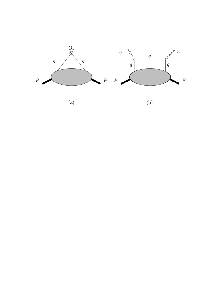
Figure 1: a) Form of the operator matrix elements in the absence of gluons. b) Form of the structure function using the OPE and neglecting the gluons both in the coefficient functions and the operator matrix elements.

Given this motivation we now consider the form of the quark (and anti-quark) operator matrix elements corresponding to Fig.1a. The contributing operators in this approximation are simply determined using the quark model to determine the coefficients $F_{2,3}$ of eq(10). Using this, the sum over operators with the operator matrix elements determined in the approximation of neglecting gluons is equivalent to evaluating the diagram in Fig.1b. The latter requires knowlege of the distribution $f_{s}(p,S,k,s)\equiv f_{s}(p^{2},k^{2},p.k,k.S,p.s)$ of quarks with polarisation $s$ within a proton. In the next section we will specify these polarisation states precisely but here we wish to continue our discussion within the framework of the OPE. The quark distributions $f_{s}(p^{2},k^{2},p.k,k.S,p.s)$ in fact provide a convenient summary of the effects of the operator matrix elements and provide the easiest way of determining the implications of the valence approximation for the general OPE. Let us note the following facts concerning the OPE:

Operators related by equations of motion are not independent. In fact Shuryak and Vainstein[8] used the equations of motion to show that, in the absence of quark masses, the twist-3 operators introduced above are equivalent to operators involving gluons only. Their general result (for massless quarks) is

$$O_{3,k} = S[\frac{g}{8}\sum_{l=0}^{n-2}i^{n-2}\bar{\psi}D_{\mu_{1}}...D_{\mu_{l}}\tilde{G}_{\sigma\mu_{l+1}}D_{\mu_{l+2}}...D_{\mu_{n-1}}\gamma_{\mu_{n}}\lambda_{k}\psi$$ (15)

$$+ \frac{g}{16}\sum_{l=0}^{n-3}i^{n-3}\bar{\psi}D_{\mu_{1}}...D_{\mu_{l}}(D_{\mu_{l+1}}\tilde{G}_{\sigma\mu_{l+2}})D_{\mu_{l+3}}...D_{\mu_{n-1}}\gamma_{\mu_{n}}\lambda_{k}\psi]$$

where $\tilde{G}_{\alpha\beta}=\frac{1}{2}\epsilon_{\alpha\beta\lambda\sigma}G^{\lambda\sigma}$.

Thus the twist-3 operator matrix elements will vanish in the valence quark approximation up to mass effects. We shall discuss the massive case shortly; in any case we may use the equations of motion to set $k^{2}=m^{2}$, the quark mass squared.

The second point is that the normalisation scale dependence of the operators is cancelled in the prediction for a physical quantity by the scale dependence of the coefficient functions $F_{2,3}$. Thus the evaluation of Fig.1b which corresponds to the full observable cross section has no scale dependence.

Putting these points together we see that the quark distributions in fact are functions of just two variables $f_{s}(p^{2},k^{2},p.k,k.S,p.s)=f_{s}(p.k,k.S)$ since $p^{2}$ and $k^{2}$ are given by the nucleon mass squared and the quark mass squared respectively and, in the relativistic quark limit, $p.s=p.k$.

Let us discuss the implications for cases of increasing complexity. First consider the trivial case of scattering off a free on-shell quark moving collinearly with the target. In this case the quark distribution $f_{s}$ is known (trivial) and the scattering amplitude is simply given by the $\gamma q$ Born diagram. Some care must be exercised in the massless limit. Since $g_{2}$ is to be determined via eq(2) (in this case $p^{\mu}$ and $S^{\mu}$ are the quark momentum and spin) we must use a massive quark with mass $m$ otherwise the factor multiplying $g_{2}(x)$ vanishes. The massless quark limit is then easily obtained by taking the limit $m\rightarrow 0$. The Born diagram gives an amplitude proportional to

$$im\epsilon_{\mu\nu\rho\sigma}q^{\rho}s^{\sigma}\delta((k+q)^{2})$$ (16)

Comparison with eq(2) immediately shows that $g_{2}=0$. How does this relate to the OPE analysis? The operators contributing simply correspond to those in the structure

$$\frac{1}{((p+q)^{2}+m^{2})}\bar{\psi}\gamma_{\mu}(/p+/q+m)\gamma_{\nu}\psi$$ (17)

The term $\psi\gamma_{\mu}(/q)\gamma_{\nu}\psi\equiv i\epsilon_{\mu\alpha\nu\sigma}q^{\alpha}\bar{\psi}\gamma_{5}\gamma^{\sigma}\psi$ when combined with the factors found expanding $(p+q)^{-2}=\sum_{i}(-2p.q/q^{2})^{i}/q^{2}$ and Fourier transforming to change the $p_{\mu}$ to a derivative acting on the quark field, immediately leads to the combination of operators $O_{2}^{\sigma\mu_{1}...\mu_{n}}+O_{3}^{\sigma\mu_{1}...\mu_{n}}$. The reason this combination arises is simply because there is no symmeterisation (or antisymmeterisation) in the Born term between the $\sigma$ index and the indices associated with the $(p.q)^{i}$ terms. As discussed above $O_{2}$ alone gives rise to the WW relations and non-vanishing $g_{2}$. Thus the vanishing of $g_{2}$ must come about through a cancellation of the contributions of $O_{2}$ and $O_{3}$. At first sight this seems impossible because of the Shuryak Vainstein relation eq(15) which suggests $O_{3}$ vanishes in the absence of gluons. However here this is not true as a careful computation of the mass effects reveals. To illustrate the point consider the simplest operators

$$O_{2}=i^{2}S_{1}\bar{\psi}\gamma_{\sigma}\gamma_{5}\partial_{\mu_{1}}\partial_{\mu_{2}}\psi$$

$$O_{3}=i^{2}SA\bar{\psi}\gamma_{\sigma}\gamma_{5}\partial_{\mu_{1}}\partial_{\mu_{2}}\psi$$ (18)

By writing $\partial_{\mu}=\{\gamma_{\mu},/\partial\}/2$ we may re-express these as

$$O_{2}=i^{2}S_{1}\bar{\psi}\gamma_{\sigma}/\partial\gamma_{\mu_{1}}\gamma_{5}\partial_{\mu_{2}}\psi$$

$$O_{3}=imSA\bar{\psi}\gamma_{\sigma}\gamma_{5}\gamma_{\mu_{1}}\partial_{\mu_{2}}\psi$$ (19)

We now take matrix elements of these operators between on-shell partons with polarisation vector $S_{\mu}$. In momentum space we have

$$<p,S|O_{2}|p,S> \propto Tr((/p+m)(1+\gamma_{5}/S)\gamma_{\sigma}\gamma_{5}/p\gamma_{\mu_{1}})p_{\mu_{2}}$$

$$= 4m(S_{\sigma}p_{\mu_{1}}+S_{\mu_{1}}p_{\sigma})p_{\mu_{2}}$$

$$<p,S|O_{3}|p,S> \propto Tr((/p+m)(1+\gamma_{5}/S)\gamma_{\sigma}\gamma_{5}\gamma_{\mu_{1}})p_{\mu_{2}}$$ (20)

$$= 4m(S_{\sigma}p_{\mu_{1}}-S_{\mu_{1}}p_{\sigma})p_{\mu_{2}}$$

Thus we see explicitly that for the combination $(O_{2}+O_{3})$ there is a cancellation between $O_{2}$ and $O_{3}$ of the term $\propto p_{\sigma}$ which is associated with $g_{2}$. This cancellation persists in the massless limit. The reason is that although the $O_{3}$ (and $O_{2}$) matrix element is formally of $O(m)$ this is cancelled by the $1/m$ behaviour of the polarisation vector $s_{\mu}\sim p_{\mu}/m$. Thus $O_{3}$ does contribute even in the limit gluons are ignored. We have somewhat belaboured our discussion of this very simple model because this point has been the source of considerable confusion in the literature.

So far our discussion has shown that $g_{2}$ vanishes in the free quark model, a well known result. Of course a model of free collinear quarks is not realistic and to determine the implications of more reasonable models we consider now the case of Fig.1b with nontrivial $f_{s}$. As we have stressed the calculation of the full diagram is completely equivalent to the use of the OPE with operator matrix elements determined in the valence approximation. Following the analysis presented above the result is given in eqs.(6) and (7) and satisfies the WW relation. To understand the origin of this relation we note that the intermediate (vertical) states of Fig.1b are on-shell quarks and the result of eqs.(6) and (7) was derived to leading order only in the quark masses. To this order the quark polarisation vector is $s_{\mu}\sim k_{\mu}/m$ and the matrix element of $O_{3}$ between the quark states vanishes simply because one cannot form an antisymmetric tensor from $k_{\mu}$ alone. This immediately implies that only $O_{2}$ contributes giving rise to the WW relation. This result again is puzzling because there is no obvious limit in which the free quark result with vanishing $g_{2}$ can be obtained i.e. why doesn’t this argument apply too in the free quark case discussed above? The answer is that the determination of $g_{2}$ requires the identification of the coefficient of the second tensor in eq(2). As we noted above this vanishes identically in the free quark limit (the approximation that $S_{\mu}\sim p_{\mu}/m$) and for this reason we had to compute $g_{2}$ in the massive quark case and take the massless limit only at the very end. In the present case however the tensor structure of eq(2) refers to the real nucleon and therefore doesn’t vanish when using the approximation $s_{\mu}\sim k_{\mu}/m$. Thus the argument showing the vanishing of the $O_{3}$ contribution applies in this case and we do indeed get the WW relation. Of course in the limit the nucleon mass is taken small and the nucleon polarisation satisfies $S_{\mu}\sim p_{\mu}/M$ the argument that $O_{3}$ vanishes fails and the WW relation would not apply. This is the limit that establishes the connection with the free quark model result for it leads to $g_{2}=0$ again. Thus we may see the WW result applies in the limit $m/M$ and $m/k_{T}$ are small while the free quark model result applies when $m\sim M$, with $m/k_{T}$ small. In the next section we extend the calculation to include mass effects to approach the region where $m/M$ and $m/k_{T}$ are not negligible.

Before leaving the OPE analysis we should comment on the role of another twist-3 operator not included in the above analysis. This is the operator

$$O_{m}=mSA\bar{\psi}\gamma_{\sigma}\gamma_{\nu}\partial_{\mu_{1}}...\partial_{\mu_{n}}\psi$$ (21)

From eq(17) we see this operator arises through the term proportional to $m$. However it is easy to check in the free quark model case that it gives rise to a gauge variant term which is cancelled by the term proportional to $/p$ in eq(17)which involves the operators $O_{2,3}$ and which have a matrix element proportional to $m$.

Our analysis of the OPE in the approximation of ignoring gluons has shown that it is equivalent to a covariant formulation of the quark parton model. As discussed in [3] this leads to a completely consistent description of both polarised and unpolarised scattering. The analysis also shows why other parton model formulations have led to contradictory results because the OPE requires the use of equations of motion to relate the various operators. This is in conflict with a parton model formulation in which the parton momentum is a fraction, $x$, of the nucleon momentum because the parton mass will then be $xM$, an $x$ dependent quantity not consistent with the equations of motion of the underlying quark states. Thus in these models contradictory results for polarised scattering are obtained (see [11] for a discussion of these results) but being in conflict with the OPE their predictions should be ignored. As a result we see that there is no remaining theoretical conflict for the case of the covariant quark parton model description of polarised scattering. Whether it provides a good phenomenological description of polarised scattering is a question for experiment.

4 Corrections from finite quark masses

Only for massless quarks is the parton polarisation vector $s^{\sigma}$ proportional to $k^{\sigma}$. In the $m\neq 0$ case the partons will, in general, have three polarisation components. Let us choose as a convenient basis the vectors $n_{i}$ given by

$$n_{1}^{\mu} = \frac{1}{mN_{1}}[(p.k)k^{\mu}-m^{2}p^{\mu}]$$

$$n_{2}^{\mu} = \frac{1}{N_{2}}\epsilon^{\mu\nu\rho\sigma}k_{\nu}S_{\rho}p_{\sigma}$$

$$n_{3}^{\mu} = \frac{1}{N_{1}N_{2}}\epsilon^{\mu\nu\rho\sigma}k_{\nu}\epsilon_{\rho\alpha\beta\gamma}k^{\alpha}S^{\beta}p^{\gamma}p_{\sigma}$$ (22)

$$= \frac{1}{N_{1}N_{2}}[M^{2}(k.S)k^{\mu}+N_{1}^{2}S^{\mu}-(p.k)(k.S)p^{\mu}]$$

where

$$N_{1} = [(p.k)^{2}-m^{2}M^{2}]^{1\over 2}$$

$$N_{2} = -[(p.k)^{2}-M^{2}(k.S)^{2}-m^{2}M^{2}]^{1\over 2}$$ (23)

In the parton rest-frame these vectors form a set of orthogonal unit 3-vectors and, in any frame, satisy $k.n_{i}=0$, $n_{i}.n_{j}=-\delta_{ij}$. In the proton rest-frame (PRF), they are given by

$$n_{1}=\frac{1}{m}(|\vec{k}|,k_{0}\hat{\vec{k}}),\quad\hat{\vec{n}}_{2}=\frac{1}{\sin\theta}(\hat{\vec{k}}\times\hat{\vec{S}}),\quad\hat{\vec{n}}_{3}=\frac{1}{\sin\theta}[\hat{\vec{k}}\times(\hat{\vec{k}}\times\hat{\vec{S}})]$$ (24)

where $\hat{\vec{k}}.\hat{\vec{S}}=\cos\theta$ and $\hat{\vec{k}},\hat{\vec{S}}$ are unit vectors in the direction of the parton momentum and proton spin respectively. The charge weighted combination of the relevant parton distributions in each direction we call $\Delta f_{i}(p,k,s)$. The vector $n_{1}$ is the longitudinal polarisation vector of the parton, $mn_{1}^{\mu}=k^{\mu}+O(m^{2}/M^{2})$ and so $\Delta f_{1}(p,k,s)$ is to be associated with the $\Delta f(p,k,s)$ of eq(5).

These $O(m^{2}/M^{2})$ corrections modify the integrand of eq(6) and since the value of $k_{T}^{2}=M^{2}[x(y-x)-m^{2}/M^{2}]$ the integrand of eq(7) is also appropriately modified. In addition, there are $O(m^{2}/M^{2})$ corrections to the limits of the integration in $y$. If we write $\alpha=m^{2}/M^{2}$ then $y_{max}=1+\alpha$ follows from constraining $(p-k)^{2}\geq 0$ while $y_{min}=x+\alpha/x$ follows from $k_{T}^{2}\geq 0$. The resulting expressions for $g_{1}$ and $g_{2}$ associated with the component $n_{1}^{\mu}$ are

$$g_{1}^{(1)}(x) = \frac{\pi M^{2}}{8}\int^{y_{max}}_{y_{min}}dy\;x(2x-y)\;(1-\frac{2\alpha}{xy})\;\tilde{h}_{1}(y)$$

$$g_{2}^{(1)}(x) = \frac{\pi M^{2}}{8}\int^{y_{max}}_{y_{min}}dy\;[x(2y-3x)+\alpha(4\frac{x}{y}-3)]\;\tilde{h}_{1}(y)$$ (25)

Here, $\tilde{h}_{1}(y)=(1-\frac{4\alpha}{y^{2}})^{-\frac{1}{2}}\int dk^{2}\tilde{f}(k^{2},y)$ where $\Delta f_{1}(p,k,S)=-(k.S)/M\;\tilde{f}(k^{2},y)$

Notice that $y_{max}\geq y_{min}$ only if $x\geq\alpha$, i.e. $g_{1,2}^{(1)}$ are zero for $x<m^{2}/M^{2}$. The above expressions do not satisfy the WW sum rules(8) but $g_{2}^{(1)}$ does satisfy the BC sum rule(9) exactly. To see this we assume that we can interchange the order of the $x,y$ integrations and use the fact that the support of $x$, for fixed $y$, is given by $x_{min}\leq x\leq x_{max}$ where $x_{min}$ and $x_{max}$ are solutions of $x^{2}-xy+\alpha=0$.

The $n_{2}^{\mu}$ component is irrelevent since it is orthogonal to $S^{\mu}$ and so $\Delta f_{2}(p,k,S)$ vanishes. The $n_{3}^{\mu}$ component does contribute however and substituting into eqs(3,4) gives the appropriate contributions to $g_{1}$ and $g_{2}$

$$g_{1}^{(3)}(x) = \pi mM^{5}\;\int^{y_{max}}_{y_{min}}dy\frac{x(y-x)-\alpha}{4N_{1}N_{2}}\int dk^{2}\Delta f_{3}(p,k,s)$$

$$g_{2}^{(3)}(x) = \pi mM^{5}\;\int^{y_{max}}_{y_{min}}dy\frac{1}{8N_{1}N_{2}}\left[\frac{y^{2}}{2}-3x(y-x)+\alpha\right]\int dk^{2}\Delta f_{3}(p,k,s)$$ (26)

where $y_{min}$, $y_{max}$ and $\alpha$ defined as above. The $g_{1}^{(3)}$ and $g_{2}^{(3)}$ defined by eq(26) satisfy analogous sum rules to the WW sum rules in the limit $\alpha\longrightarrow 0$. Provided $\Delta f_{3}\propto N_{2}$, which is true in any reasonable model (see below), we can write in this limit

$$\int_{0}^{1}dxx^{n-1}\left[\frac{(n-1)(n-2)}{4n}g_{1}^{(3)}(x)-g_{2}^{(3)}(x)\right]=0$$ (27)

This relation is interesting in that not only is the BC sum rule satisfied but also the first moment of $g_{2}^{(3)}$ vanishes which implies that $g_{2}^{(3)}$ is suppressed in general. When $\alpha\neq 0$ the $n=1,2$ sum rules both survive exactly.

The above expressions, eq(25) and eq(26), are quite general. As they involve two distribution functions, they do not lead to a relation between $g_{1}$ and $g_{2}$. However, as we now discuss, the covariant parton model allows us to develop a plausible model to describe the source of the parton polarisation in the proton and hence to relate $\Delta f_{1}(p,k,s)$ and $\Delta f_{3}(p,k,s)$. How are the partons polarised? Ultimately it is due to the interaction with the external magnetic field which causes the proton spin, through the interaction of the proton magnetic moment, to align with the field. At the parton level, while they too will interact directly with the magnetic field, they will also have spin-spin interations which align the individual parton spins. The latter interaction, being due to the strong force, may be expected to dominate the relative parton spin alignment which is what relates $\Delta f_{1}(p,k,s)$ and $\Delta f_{3}(p,k,s)$. Since, on average, any combination of parton spins is proportional to the proton spin we are led to a model in which the relative magnitude of $\Delta f_{i}$ is due to the spin-spin interaction between the partons themselves, the interaction being proportional to the scalar product of the individual parton spin with the proton spin. Thus we have

$$\Delta f_{i}(p,k,S)=(n_{i}.S)\;m\;\hat{f}(p.k,k^{2})$$ (28)

From eq(22) we have

$$m\;(n_{1}.S) = \frac{(p.k)(k.S)}{N_{1}}$$

$$m\;(n_{2}.S) = 0$$

$$m\;(n_{3}.S) = -m\;\frac{N_{2}}{N_{1}}$$ (29)

We see that factoring out $(k.S)$ in eq(5) in the massless case is consistent with this model. The factor $m$ on the rhs of eq(28) ensures the desired limit for the $n_{1}^{\mu}$ contribution as $m\longrightarrow 0$. We can now write $\Delta f_{3}$ in terms of $\tilde{f}$,

$$\Delta f_{3}(p,k,S)=\frac{mN_{2}}{M(p.k)}\;\tilde{f}(k^{2},y)$$ (30)

and substitute into eqs(26) to get

$$g_{1}^{(3)}(x) = \pi m^{2}\;\int^{y_{max}}_{y_{min}}dy\left[\frac{x(y-x)-\alpha}{y^{2}}\right]\tilde{h}_{1}(y)$$

$$g_{2}^{(3)}(x) = \pi m^{2}\;\int^{y_{max}}_{y_{min}}dy\frac{1}{2y^{2}}\left[\frac{y^{2}}{2}-3x(y-x)+\alpha\right]\tilde{h}_{1}(y)$$ (31)

Thus $g_{1}(x)=g_{1}^{(1)}(x)+g_{1}^{(3)}(x)$ and $g_{2}(x)=g_{2}^{(1)}(x)+g_{2}^{(3)}(x)$ are determined by a single function once again, as in the $m=0$ case. The resultant prediction for $g_{2}(x)$ in terms of the measured $g_{1}(x)$ is pursued in the next section.

In leading order the final form of the quark mass effects consists of two pieces. The first which starts at $O(\frac{m^{2}}{M^{2}})$ comes simply from imposing parton kinematics on the scattering process. The second, of $O(\frac{m}{M})$, is given in eq(26) and comes from the transverse polarisation states. The question immediately arises whether it is the constituent or current mass that is relevant. At the level of the quark parton model itself this cannot be answered as it is the QCD interactions that cause masses to “run”. However one may make an educated guess as to the most appropriate choice. The calculation of the parton model process requires, for gauge invariance, that the mass of the intermediate parton be the same as that of the initial parton. The former should certainly be taken as the current-quark mass at the scale $Q^{2}$ since the large momentum involved in the deep inelastic scattering process flows through it. Hence the struck quark mass should also be taken to be the current-quark mass. As a result we expect the corrections of $O(\frac{m}{M})$ in eq(26) to relate to the current quark mass. The kinematic corrections however have two origins. The first, due to the $y_{min}$ cut and from the form of the parton momentum $k$, comes from putting the struck parton on mass shell and again for consistency should be taken to be the current-quark mass. The second, the $y_{max}$ cut, comes from imposing parton kinematics on the intermediate states in the lower bob of Fig 1b. This must surely be the constituent mass as no large momenta are involved. However, in practice, the former effects are the most important and hence we expect the dominant mass effects to be assocated with the current quark mass (in the phenomenological analysis given below we make no distinction between the various masses - consistent with the parton model interpretation - but, following this discussion, we expect the masses should be of current quark magnitude).

5 Phenomenological analysis

Figure 2: Fit to the data on $g_{1}(x)$ from refs(4,5,6) using eq.(6) and the comparison of the resulting prediction for $g_{2}(x)$ from eq.(7) with the preliminary data of ref(1). This is the $m=0$ case.

Fig.2 shows the present situation for the experimental measurements by SLAC[4], EMC[5] and SMC[6] for $g_{1}(x)$ together with the recent preliminary measurements of $g_{2}(x)$ at SLAC[1]. The range of $Q^{2}$ over which all the measurements are taken is fairly wide and, in principle, one should try to take account of possibly sizeable $Q^{2}$ variation at fixed $x$ values. However we do not tackle this here as we are concerned here only with the challenge of trying to predict the size and shape of $g_{2}(x)$ from that of $g_{1}(x)$ at some canonical value of $Q^{2}$ where the parton model may apply and, by definition, QCD corrections are assumed to be small.

Also shown in Fig.2 is the expected $m=0$ prediction for $g_{2}(x)$ where we fit to the data on $g_{1}(x)$ using the expression eq(6) with an assumed form for $\tilde{h}(y)=ax^{-b}(1-x)^{c}$ which is then inserted into eq(7) to give $g_{2}(x)$. That is, the curve on Fig.2 is the prediction for $g_{2}(x)$ given by the WW relation eq(1). We find $b\sim 3$ and $c\sim 1$. Certainly at large $x$ it is encouraging to see the preliminary $g_{2}$ data lying close to the WW expectation. Note that, from eq(1), the prediction for $g_{2}(x)$ at any $x$ value depends only on values of $x$ at and above that value and so is not sensitive to uncertainties in the small $x$ region. Likewise, parametrisations of the distributions $\tilde{h}(y)$ are not required to satisy various theoretical conjectures for the small $x$ behaviour since this region is quite irrelevant to our concerns here.

Figure 3: Fits to the data on $g_{1}(x)$ from refs(4,5,6) using eqs.(25,31) for $m/M$ up to 0.2 and the comparison of the resulting predictions for $g_{2}(x)$ from eqs.(25,31) with the preliminary data of ref(1).

Figure 4: The two components $g_{i}^{(1)}(x)$ and $g_{i}^{(3)}(x)$ for the fits shown in Fig.3

Our conclusion following from Fig.2 is that the preliminary $g_{2}$ data, albeit with relatively large errors, is consistent with WW relation and hence, within the framework of the covariant partom model, consistent with a light quark mass of zero. The next step is to ask if the data are also consistent with a sizeable quark mass.

To answer this question, we carried out fits to $g_{1}(x)=g_{1}^{(1)}(x)+g_{1}^{(3)}(x)$ using eqs.(25,31) for $m/M$ up to 0.2 and a similar parametrisation for $\tilde{h}(y)$ as in the $m=0$ case above. The resulting fits, together with the corresponding predictions for $g_{2}(x)=g_{2}^{(1)}(x)+g_{2}^{(3)}(x)$ are shown in Fig.3. The quality of the fits is good provided $m/M\lower 3.01385pt\hbox{$\;\stackrel{{\scriptstyle\textstyle<}}{{\sim}}\;$}0.04$, however the resulting $\chi^{2}$ never improves on the value of 59 for 50 data points achieved by the $m=0$ fit. This remains true even when more complicated parametrisations of $\tilde{h}(y)$ are considered.

The components of $g_{1}(x)$ and $g_{2}(x)$ associated with the $n_{1}^{\mu}$ and $n_{3}^{\mu}$ components of the parton polarisation are shown in Fig.4. As $m/M$ increases, $g_{1}^{(3)}(x)$ grows at low $x$ $-$ the suppression of $O(m^{2}/M^{2})$ is largely offset by the denominator $y^{2}$ in the integrand $-$ and tends to spoil the quality of the fits. Notice in Fig.4 that each component of $g_{2}(x)$ correctly integrates to zero and note how $g_{2}^{(3)}(x)$ is suppressed relative to $g_{2}^{(1)}(x)$ due to the vanishing of the first moment.

To quantify the violation of the WW sum rules in this particular model for the quark mass effects we consider the ratio $r_{n}$ given by

$$r_{n}=\frac{\int^{1}_{0}dx\;x^{n-1}\;\big{[}\frac{n-1}{n}g_{1}(x)+g_{2}(x)\big{]}}{\int^{1}_{0}dx\;x^{n-1}\;\big{[}\frac{n-1}{n}g_{1}(x)\big{]}}$$ (32)

That is, $r_{n}$ is the WW moment normalised by the $g_{1}$ contribution to that moment. Up to values of $m/M$ where the model is able to successfully describe the data, $r_{n}$ can be used as a direct measure of the quark mass. For values of $m/M=0.01,\;0.02,\;0.04$ we get $r_{2}=1.2,\;3.4,\;9.0\%$.

As the precision of the SLAC $g_{2}$ measurement increases, we expect that a phenomenological analysis such as this can offer a new and practical procedure for testing whether the quark model is a good approximation.

Acknowledgement

We would like to thank G. Altarelli and K. Ellis for useful discussions.

References

- [1] SLAC E143 collaboration: C. Prescott talk at Erice meeting on the Spin Structure of the Nucleon, Aug. 1995.
- [2] S. Wandzura and F. Wilczek, Phys. Lett. B72(1977) 195.
- [3] J.D. Jackson, G.G. Ross and R.G. Roberts, Phys. Lett. B226(1989) 159.
- [4] SLAC E143 collaboration: K. Abe et al., Phys. Rev. Lett. 74(1995) 74.
- [5] EM collaboration: J. Ashman et al., Nucl. Phys. B328(1989) 1.
- [6] SM collaboration: D. Adams et al., Phys. Lett. B329(1994) 399.
- [7] R.L. Heimann, Nucl. Phys. B64(1973) 439.
- [8] E.V. Shuryak and A.I. Vainshtein, Nucl. Phys. B201(1982) 141.
- [9] R.L. Jaffe, Comm. Nucl. Part. Phys. 14(1991) 239.
- [10] R.L. Jaffe and X. Ji, Phys. Rev. D43(1991) 724.
- [11] M. Anselmino, A. Efremov and E. Leader, Phys. Rep. 261(1995) 1.
- [12] H. Burkhadt and W.N. Cottingham, Ann. Phys. 56(1990) 453.
- [13] G.Altarelli, B.Lampe, P.Nason and G.Ridolfi, Phys. Lett. B334(1994)187