Looking Beyond the Standard Model
through
Precision Electroweak Physics

Abstract

The most important hint of physics beyond the Standard Model (SM) from the 1995 precision electroweak data is that the most precisely measured quantities, the total, leptonic and hadronic decay widths of the $Z$ and the effective weak mixing angle, $\sin^{2}\theta_{W}$, measured at LEP and SLC, and the quark-lepton universality of the weak charged currents measured at low energies, all agree with the predictions of the SM at a few $\times 10^{-3}$ level. By taking into account the above constraints I examine implications of three possible disagreements between experiments and the SM predictions. It is difficult to interpret the 11% (2.5-$\sigma$) deficit of the $Z$-partial-width ratio $R_{c}=\Gamma_{c}/\Gamma_{h}$, since it either implies an unacceptably large $\alpha_{s}$ or a subtle cancellation among hadronic $Z$ decay widths in order to keep all the other successful predictions of the SM. The 2% (3-$\sigma$) excess of the ratio $R_{b}=\Gamma_{b}/\Gamma_{h}$ may indicate the presence of a new rather strong interaction, such as the top-quark Yukawa coupling in the supersymmetric (SUSY) SM or a new interaction responsible for the large top-quark mass in the Technicolor scenario of dynamical electroweak symmetry breaking. Another interpretation may be additional tree-level gauge interactions that couple only to the third generation of fermions. A common consequence of these attempts is a rather small $\alpha_{s}$, $\alpha_{s}(m_{Z})_{\overline{\rm MS}}=0.104\pm 0.08$. The 0.17% (1-$\sigma$) deficit of the CKM unitarity relation $|V_{ud}|^{2}+|V_{us}|^{2}+|V_{ub}|^{2}=1$ may indicate light sleptons and gauginos in the minimal SUSY-SM. None of the above disagreements are, however, convincing at present.

KEK–TH–463

KEK preprint 95–186

January 1996

H

Looking Beyond the Standard Model
through
Precision Electroweak Physics

Kaoru Hagiwara

Theory Group, KEK, 1-1 Oho, Tsukuba, Ibaraki 305, Japan

ABSTRACT

The most important hint of physics beyond the Standard Model (SM) from the 1995 precision electroweak data is that the most precisely measured quantities, the total, leptonic and hadronic decay widths of the $Z$ and the effective weak mixing angle, $\sin^{2}\theta_{W}$, measured at LEP and SLC, and the quark-lepton universality of the weak charged currents measured at low energies, all agree with the predictions of the SM at a few $\times 10^{-3}$ level. By taking into account the above constraints I examine implications of three possible disagreements between experiments and the SM predictions. It is difficult to interpret the 11% (2.5-$\sigma$) deficit of the $Z$-partial-width ratio $R_{c}=\Gamma_{c}/\Gamma_{h}$, since it either implies an unacceptably large $\alpha_{s}$ or a subtle cancellation among hadronic $Z$ decay widths in order to keep all the other successful predictions of the SM. The 2% (3-$\sigma$) excess of the ratio $R_{b}=\Gamma_{b}/\Gamma_{h}$ may indicate the presence of a new rather strong interaction, such as the top-quark Yukawa coupling in the supersymmetric (SUSY) SM or a new interaction responsible for the large top-quark mass in the Technicolor scenario of dynamical electroweak symmetry breaking. Another interpretation may be additional tree-level gauge interactions that couple only to the third generation of fermions. A common consequence of these attempts is a rather small $\alpha_{s}$, $\alpha_{s}(m_{Z})_{\overline{\rm MS}}=0.104\pm 0.08$. The 0.17% (1-$\sigma$) deficit of the CKM unitarity relation $|V_{ud}|^{2}+|V_{us}|^{2}+|V_{ub}|^{2}=1$ may indicate light sleptons and gauginos in the minimal SUSY-SM. None of the above disagreements are, however, convincing at present.

Talk presented at Yukawa International Seminar (YKIS) ’95
“From the Standard Model to Grand Unified Theories”
Kyoto, Japan, August 21–25, 1995

1 Introduction

Despite the firm theoretical belief that the Standard Model (SM) of the electroweak interactions is merely an effective low-energy description of a more fundamental theory, high-energy experiments have so far been unable to establish a signal of new physics. Naturalness of the dynamics of the electroweak-gauge-symmetry breakdown suggests that the energy scale of new-physics should lie below or at $\sim 1$ TeV. Because of this relatively low new-physics scale, there has been a hope that hints of new physics beyond the SM might be found as quantum effects affecting precision electroweak observables.

In response to such general expectations the experimental accuracy of the electroweak measurements has steadily been improved in the past several years, reaching the $10^{-5}$ level for $m_{Z}$, a few $\times 10^{-3}$ level for the total and some of the partial $Z$ widths, and the $10^{-2}$ level for the asymmetries at LEP and SLC. Because of partial cancellation in the observable asymmetries at LEP and SLC, their measurements at the $10^{-2}$ level determine the effective electroweak mixing parameter, $\sin^{2}\theta_{W}$, at the $10^{-3}$ level. Therefore, by choosing the fine structure constant, $\alpha$, the muon-decay constant, $G_{F}$, and $m_{Z}$ as the three inputs whose measurement error is negligibly small, we can test the predictions of the SM at a few $\times 10^{-3}$ level. Accuracy of experiments has now reached the level where new physics contributions to quantum corrections can be probed.

In this report I would like to summarize the electroweak measurements that were reported as preliminary results for the 1995 Summer Conferences[1, 2, 3] from a theorist’s point of view[4] and to examine their implications on our search for new physics. In Section 2 we summarize the latest electroweak results at LEP, SLC, the Tevatron, and at low energies. These data are analysed in the general ${\rm SU(2)_{L}\times U(1)_{Y}}$ model framework[5]. In Section 3 we discuss the nature of the $R_{b}$ and $R_{c}$ ‘crisis’ in detail. In Section 4 I introduce several theoretical attempts to explain the observed 2% (3-$\sigma$) excess in $R_{b}$. In Section 5 I examine implications of a possible (1-$\sigma$) violation of the quark-lepton universality in the low-energy charged-current experiments. Section 6 summarises our findings.

2 The 1995 Precision Electroweak Data

In this section we analyse the preliminary electroweak results[1, 2, 3] presented at the 1995 summer conferences in the general ${\rm SU(2)_{L}\times U(1)_{Y}}$ model framework[5]. We allow a new physics contribution to the $S$, $T$, $U$ parameters[6] of the electroweak gauge-boson-propagator corrections as well as to the $Zb_{L}b_{L}$ vertex form factor, $\bar{\delta}_{b}(m_{Z}^{2})$, but otherwise we assume the SM contributions dominate the corrections. We take the strengths of the QCD and QED couplings at the $m_{Z}$ scale, $\alpha_{s}(m_{Z})$ and $\bar{\alpha}(m_{Z}^{2})$, as external parameters of the fits so that implications of their precise measurements on electroweak physics are manifestly shown. Those who are familiar with the framework of Ref.hhkm may skip the following subsection.

2.1 Brief Review of Electroweak Radiative Corrections in $\rm{SU(2)_{L}\times U(1)_{Y}}$ Models

The propagator corrections in the general $\rm{SU(2)_{L}\times U(1)_{Y}}$ models can conveniently be expressed in terms of the following four effective charge form-factors[5]:

(1a)

(1b)

(1c)

(1d)

where $\overline{\Pi}_{T,V}^{AB}(q^{2})\equiv[\overline{\Pi}_{T}^{AB}(q^{2})\!-\!\overline{\Pi}_{T}^{AB}(m_{V}^{2})]/(q^{2}\!-\!m_{V}^{2})$ are the propagator correction factors that appear in the $S$-matrix elements after the mass renormalization is performed, and $\hat{e}\equiv\hat{g}\hat{s}\equiv\hat{g}_{Z}\hat{s}\hat{c}$ are the $\overline{\rm MS}$ couplings. The ‘overlines’ denote the inclusion of the pinch terms[7, 8, 9], which make these effective charges useful[9, 5, 10] even at very high energies ($|q^{2}|\gg m_{Z}^{2}$). The amplitudes are then expressed in terms of these charge form-factors plus appropriate vertex and box corrections. In our analysis[5] we assume that all the vertex and box corrections are dominated by the SM contribution except for the $Zb_{L}b_{L}$ vertex,

$$\Gamma_{L}^{Zbb}(q^{2})=-\hat{g}_{Z}\{-\frac{1}{2}[1+\bar{\delta}_{b}(q^{2})]+\frac{1}{3}\hat{s}^{2}[1+\Gamma_{1}^{b_{L}}(q^{2})]\},$$ (2)

for which the function $\bar{\delta}_{b}(m_{Z}^{2})$ is allowed to take an arbitrary value. The charge form-factors and $\bar{\delta}_{b}(m_{Z}^{2})$ can then be extracted from the experimental data, and the extracted values can be compared with various theoretical predictions.

We can define[5] the $S$, $T$ and $U$ variables in terms these effective charges,

$$\frac{\bar{s}^{2}(m_{Z}^{2})\bar{c}^{2}(m_{Z}^{2})}{\bar{\alpha}(m_{Z}^{2})}-\frac{4\,\pi}{\bar{g}_{Z}^{2}(0)} \equiv \;\frac{S}{4}\,,$$ (3a)

$$\frac{\bar{s}^{2}(m_{Z}^{2})}{\bar{\alpha}(m_{Z}^{2})}\quad-\frac{4\,\pi}{\bar{g}_{W}^{2}(0)} \equiv \frac{S+U}{4}\,,$$ (3b)

$$1\;-\,\frac{\bar{g}_{W}^{2}(0)}{m_{W}^{2}}\frac{m_{Z}^{2}}{\bar{g}_{Z}^{2}(0)} \equiv \;\alpha T\,,$$ (3c)

where $\bar{\alpha}(q^{2})\!\equiv\!\bar{e}^{2}(q^{2})/4\pi$, and it is clear that these variables measure deviations from the naive universality of the electroweak gauge couplings. They receive contributions from both the SM radiative effects as well as new physics contributions. The original $S$, $T$, $U$ variables of Ref.stu are obtained in Ref.hhkm approximately by subtracting the SM contributions (at $m_{H}=1000$ GeV).

For a given electroweak model we can calculate the $S$, $T$, $U$ parameters ($T$ is a free parameter in models without custodial SU(2) symmetry), and the charge form-factors are then fixed by the following identities[5]:

$$\frac{1}{\bar{g}_{Z}^{2}(0)} = \frac{1+\bar{\delta}_{G}-\alpha\,T}{4\,\sqrt{2}\,G_{F}\,m_{Z}^{2}}\,,$$ (4a)

$$\bar{s}^{2}(m_{Z}^{2}) = \frac{1}{2}-\sqrt{\frac{1}{4}-\bar{\alpha}^{2}(m_{Z}^{2})\biggl{(}\frac{4\,\pi}{\bar{g}_{Z}^{2}(0)}+\frac{S}{4}\biggr{)}}\,,$$ (4b)

$$\frac{4\,\pi}{\bar{g}_{W}^{2}(0)} = \frac{\bar{s}^{2}(m_{Z}^{2})}{\bar{\alpha}^{2}(m_{Z}^{2})}-\frac{1}{4}\,(S+U)\,.$$ (4c)

Here $\bar{\delta}_{G}$ ($\bar{\delta}_{G}=0.0055$ in the SM) is the vertex and box correction to the muon lifetime[11] after subtraction of the pinch term[5]:

$$G_{F} = \frac{\bar{g}_{W}^{2}(0)+\hat{g}^{2}\bar{\delta}_{G}}{4\,\sqrt{2}m_{W}^{2}}\,.$$ (5)

It is clear from the above identities that, once we know $T$ and $\bar{\delta}_{G}$ in a given model, we can predict $\bar{g}_{Z}^{2}(0)$, and then, by knowing $S$ and $\bar{\alpha}(m_{Z}^{2})$, we can calculate $\bar{s}^{2}(m_{Z}^{2})$, and finally, by knowing $U$, we can calculate $\bar{g}_{W}^{2}(0)$. Since $\bar{\alpha}(0)=\alpha$ is known precisely, all four charge form-factors are then fixed at one $q^{2}$ point. The $q^{2}$-dependence of the form factors should also be calculated in a given model, but it is less dependent on physics at very high energies[5]. In the following analysis we assume that the SM contribution governs the running of the charge form-factors between $q^{2}=0$ and $q^{2}=m_{Z}^{2}$. We can now predict all the neutral-current amplitudes in terms of $S$ and $T$, and an additional knowledge of $U$ gives the $W$ mass via Eq.(5).

We should note here that our prediction for the effective mixing parameter, $\bar{s}^{2}(m_{Z}^{2})$, is not only sensitive to the $S$ and $T$ parameters but also to the precise value of $\bar{\alpha}(m_{Z}^{2})$. This is the reason why the predictions for the asymmetries measured at LEP/SLC and, consequently, the experimental constraint on $S$ extracted from the asymmetry data are dependent on $\bar{\alpha}(m_{Z}^{2})$. In order to parametrize the uncertainty in our evaluation of $\bar{\alpha}(m_{Z}^{2})$, the parameter $\delta_{\alpha}$ is introduced in Ref.hhkm as follows:

$$\delta_{\alpha}\equiv 1/\bar{\alpha}(m_{Z}^{2})-128.72\,.$$ (6)

We show in Table 1 the results of the four recent updates[13, 14, 15, 16] on the hadronic contribution to the running of the effective QED coupling. Three definitions of the running QED coupling are compared. I remark that our simple formulae (2.1) and (2.1) are valid only if one includes all the fermionic and bosonic contributions to the propagator corrections. There is no discrepancy among the four recent estimates in Table 1, where small differences are attributed to the use of perturbative QCD for constraining the magnitude of medium energy data[13] or to a slightly different set of input data[14]. For more detailed discussions I refer the readers to an excellent review by Takeuchi[18]. In the following analysis we take the estimate of Ref.eidjeg95 ($\delta_{\alpha}=0.03\pm 0.09$) as the standard, and we show the sensitivity of our results to $\delta_{\alpha}-0.03$.

Table 1: The running QED coupling at the $m_{Z}$ scale in the three schemes. $\alpha(m_{Z}^{2})_{\rm l.f.}$ contains only the light fermion contributions to the running of the QED coupling constant between $q^{2}\!=\!0$ and $q^{2}\!=\!m_{Z}^{2}$. $\alpha(m_{Z}^{2})_{\rm f}$ contains all fermion contributions including the top-quark. $m_{t}\!=\!175$ GeV and $\alpha_{s}(m_{Z})\!=\!0.12$ are assumed in the perturbative two-loop correction[17]. $\bar{\alpha}(m_{Z}^{2})$ contains also the $W$-boson-loop contribution[5] including the pinch term[7, 8]. $\delta_{\alpha}\!\equiv\!1/\bar{\alpha}(m_{Z}^{2})\!-\!128.72$.

	$1/\alpha(m_{Z}^{2})_{\rm l.f.}$	$1/\alpha(m_{Z}^{2})_{\rm f}$	$1/\bar{\alpha}(m_{Z}^{2})$	$\delta_{\alpha}$
Martin-Zeppenfeld ’94[13]	$128.98\pm 0.06$	$128.99\pm 0.06$	$128.84\pm 0.06$	$0.12\pm 0.06$
Swartz ’95[14]	$128.96\pm 0.06$	$128.97\pm 0.06$	$128.82\pm 0.06$	$0.10\pm 0.06$
Eidelman-Jegerlehner ’95[15]	$128.89\pm 0.09$	$128.90\pm 0.09$	$128.75\pm 0.09$	$0.03\pm 0.09$
Burkhardt-Pietrzyk ’95[16]	$128.89\pm 0.10$	$128.90\pm 0.10$	$128.76\pm 0.10$	$0.04\pm 0.10$

Once we know $\bar{\alpha}(m_{Z}^{2})$ the charge form-factors in Eq.(2.1) can be calculated from $S$, $T$, $U$. The following approximate formulae[5] are useful:

$$\bar{g}_{Z}^{2}(0) \approx 0.5456\hphantom{+0.0036\,S}\;\,+0.0040\,T^{\prime}\,,$$ (7a)

$$\bar{s}^{2}(m_{Z}^{2}) \approx 0.2334+0.0036\,S-0.0024\,T^{\prime}\hphantom{+0.0035\,U}\;\,-0.0026\,\delta_{\alpha}\,,\qquad$$ (7b)

$$\bar{g}_{W}^{2}(0) \approx 0.4183-0.0030\,S+0.0044\,T^{\prime}+0.0035\,U+0.0014\,\delta_{\alpha}\,,\qquad$$ (7c)

where we note that the predictions depend on $T$ only through the combination[5]

$$T^{\prime}\equiv T+(0.0055-\bar{\delta}_{G})/\alpha\,.$$ (8)

The values of $\bar{g}_{Z}^{2}(m_{Z}^{2})$ and $\bar{s}^{2}(0)$ are then calculated from $\bar{g}_{Z}^{2}(0)$ and $\bar{s}^{2}(m_{Z}^{2})$ above, respectively, by assuming the SM running of the form-factors. The $Z$ widths are sensitive to $\bar{g}_{Z}^{2}(m_{Z}^{2})$, which can be obtained from $\bar{g}_{Z}^{2}(0)$ in the SM approximately by

$${1}/{\bar{g}_{Z}^{2}(m_{Z}^{2})}\approx{1}/{\bar{g}_{Z}^{2}(0)}-0.02390+({2.41}/{m_{t}^{2}})+({1.73}/{m_{H}^{2}})$$ (9)

when $m_{t}({\,\rm GeV})>150$ and $m_{H}({\,\rm GeV})>100$. Details of the following analysis will be reported elsewhere[19].

2.2 Key Observations from the 1995 Electroweak Data

The 1995 update of the precision electroweak data are found in the LEP Electroweak Working Group reports[1, 2] in which preliminary results from LEP, SLC and the Tevatron are combined. Its concise summary is given in Ref.lp95_hag.

I would like to summarize the results by the following four key observations:

• The three line-shape parameters, $\Gamma_{Z}$, $\sigma_{h}^{0}$ and $R_{l}$, are now measured with an accuracy better than 0.2%.

  $${\Delta\Gamma_{Z}}/{\Gamma_{Z}} = -0.0010\pm 0.0013\,,$$ (10a)

  $${\Delta\sigma_{h}^{0}}/{\sigma_{h}^{0}} = \phantom{-}0.0006\pm 0.0019\,,$$ (10b)

  $${\Delta R_{l}}/{R_{l}} = \phantom{-}0.0015\pm 0.0015\,,$$ (10c)

  where $\Delta$ gives the difference between the data and the reference SM predictions[5] for $m_{t}=175$ GeV, $m_{H}=100$ GeV, $\alpha_{s}=0.12$ and $\delta_{\alpha}=0.03$. We should note here that the above three most accurately measured line-shape parameters constrain the $Z$ partial widths $\Gamma_{l}$, $\Gamma_{h}$ and $\Gamma_{\rm inv}$ accurately;

  $$\Delta\Gamma_{h}/\Gamma_{h} = \phantom{-}0.0001\pm 0.0017\,,$$ (11a)

  $$\Delta\Gamma_{l}/\Gamma_{l} = -0.0013\pm 0.0016\,,$$ (11b)

  $$\Delta\Gamma_{\rm inv}/\Gamma_{\rm inv} = -0.004\pm 0.005\,,$$ (11c)

  because they are three independent combinations of the above three widths, $\Gamma_{Z}=\Gamma_{h}\!+\!\Gamma_{l}\!+\!\Gamma_{\rm inv}$, $R_{l}=\Gamma_{h}/\Gamma_{l}$, and $\sigma_{h}^{0}=(12\pi/m_{Z}^{2})\Gamma_{h}\Gamma_{l}/\Gamma_{Z}^{2}$.

• Detailed tests[1, 3] of the $e$-$\mu$-$\tau$ universality show that any hint of universality violation in the 1994 data is now disappearing.

  $${\Delta\Gamma_{\tau}}/{\Gamma_{\tau}} = \phantom{-}0.000\pm 0.0035\,,$$ (12a)

  $${\Delta\Gamma_{\nu_{\tau}}}/{\Gamma_{\nu_{\tau}}} = -0.012\pm 0.015\,,$$ (12b)

  $${\Delta A_{\tau}}/{A_{\tau}} = -0.04\pm 0.05\,,$$ (12c)

  $${\Delta A_{\rm FB}^{\tau}}/{A_{\rm FB}^{\tau}} = \phantom{-}0.23\pm 0.14\,.$$ (12d)

  The result for $\Gamma_{\nu_{\tau}}$ is obtained from Eq.(11c) by assuming $\Gamma_{\rm inv}=\Gamma_{\nu_{e}}+\Gamma_{\nu_{\mu}}+\Gamma_{\nu_{\tau}}$ with the SM values for $\Gamma_{\nu_{e}}$ and $\Gamma_{\nu_{\mu}}$. Although the $\tau$ forward-backward asymmetry is still 1.7$\sigma$ away from the SM prediction, the accuracy of the measurement is still poor (14%), and its significance is overshadowed by the excellent agreements in the partial widths $\Gamma_{\tau}$, $\Gamma_{\nu_{\tau}}$ and the $\tau$ polarization asymmetry, $A_{\tau}$, which are measured at the 0.35%, 1.5% and 5% level, respectively.

  

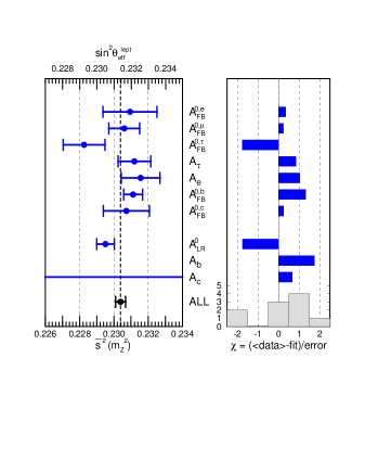
  Figure 1: The effective electroweak mixing parameter[5] ${\bar{s}}^{2}(m_{Z}^{2})$ is determined from all the asymmetry data from LEP and SLC. The effective parameter $\sin^{2}\theta_{\rm eff}^{\rm lept}$ of the LEP Electroweak Working Group[1] is obtained accurately[5] as $\sin^{2}\theta_{\rm eff}^{\rm lept}={\bar{s}}^{2}(m_{Z}^{2})+0.0010$. The data on $A_{b}$ is off the scale.

• All the asymmetry data, including the left-right beam-polarization asymmetry, $A_{\rm LR}$, from SLC, are now consistent with each other. I show in Fig. 1 the result of the one-parameter fit to all the asymmetry data in terms of the effective electroweak mixing-angle, $\bar{s}^{2}(m_{Z}^{2})$. The fit gives

  $$\bar{s}^{2}(m_{Z}^{2})=0.23039\pm 0.00029$$ (13)

  with $\chi^{2}_{\rm min}/({\rm d.o.f.})=13.0/(9)$. The updated measurements of the asymmetries agree well (16%CL) with the ansatz that the asymmetries are determined by the universal electroweak mixing parameter. Even though $\bar{s}^{2}(m_{Z}^{2})$ determined from the left-right beam-polarization asymmetry of the $b$-quark forward-backward asymmetry, $A_{b}$, is off the scale, its significance is still moderate because of its large measurement error, $\Delta A_{b}/A_{b}=-0.10\pm 0.06$.

• The only data which disagree significantly with the predictions of the SM are the two ratios $R_{b}=\Gamma_{b}/\Gamma_{h}$ and $R_{c}=\Gamma_{c}/\Gamma_{h}$. Here $\Gamma_{q}$ denotes the partial $Z$ decay widths into $q\bar{q}$-initiated hadronic final states, and $\Gamma_{h}$ denotes the hadronic $Z$ decay width. $R_{b}$ is larger than the reference SM prediction by 3% (3.7-$\sigma$), whereas $R_{c}$ is smaller than the prediction by 11% (2.5-$\sigma$). The trends of larger $R_{b}$ and smaller $R_{c}$ existed in the combined data for the past few years, but their significance grew considerably in the 1995 update.

I remark here that the interpretation of the possible deviations from the SM in the last item is severely restricted by the remaining excellent successes of the SM listed above. I will show in Section 3 that it is difficult to accommodate the $R_{c}$ data with all the other successes of the SM, but the $R_{b}$ data can easily be accommodated by modifying only the $Zb_{L}b_{L}$ vertex.

In this section I show results of the analysis[19] where all the vertex and box corrections, except for the $Zb_{L}b_{L}$ vertex function, $\bar{\delta}_{b}(m_{Z}^{2})$, are dominated by the SM contributions. All the LEP and SLC results are then fitted by the four parameters $\bar{g}_{Z}^{2}(m_{Z}^{2})$, $\bar{s}^{2}(m_{Z}^{2})$, $\bar{\delta}_{b}(m_{Z}^{2})$ and $\alpha_{s}=\alpha_{s}(m_{Z})_{\overline{\rm MS}}$. We find[19]

$$\left.\begin{array}[]{ll}\bar{g}_{Z}^{2}(m_{Z}^{2})&\!\!=0.55556-0.00049\,{\textstyle\frac{\alpha_{s}^{\prime}-0.1081}{0.0043}}\pm 0.00072\\[2.84526pt] \bar{s}^{2}(m_{Z}^{2})&\!\!=0.23041+0.00004\,{\textstyle\frac{\alpha_{s}^{\prime}-0.1081}{0.0043}}\pm 0.00029\end{array}\right\}\,\,\rho_{\rm corr}=0.23,$$ (14c)

$$\quad\chi^{2}_{\rm min}=15.6+\biggl{(}\frac{\alpha_{s}^{\prime}-0.1081}{0.0043}\biggr{)}^{2}+\biggl{(}\frac{\bar{\delta}_{b}-0.0025}{0.0042}\biggr{)}^{2}\,,$$ (14d)

where

$$\alpha_{s}^{\prime}=\alpha_{s}(m_{Z})_{\overline{\rm MS}}\,+1.54\,\bar{\delta}_{b}(m_{Z}^{2})$$ (15)

is the combination[5] that appears in the theoretical prediction for $\Gamma_{h}$. As a consequence of the $R_{b}$ data the best fit is obtained at $\bar{\delta}_{b}(m_{Z}^{2})=0.0025$ and $\alpha_{s}=0.1043$. Within the SM, however, the form factor $\bar{\delta}_{b}(m_{Z}^{2})$ takes only a negative value ($\bar{\delta}_{b}(m_{Z}^{2})\hbox to0.0pt{\lower 3.5pt\hbox{$\mathchar 0\relax\sim$}\hss}\raise 1.0pt\hbox{$<$}-0.03$), and its magnitude grows quadratically with $m_{t}$. It can be parametrized accurately in the region 100$<m_{t}({\,\rm GeV})<$200 as[5]

$$\bar{\delta}_{b}(m_{Z}^{2})_{\rm SM}\approx-0.00099-0.00211(\frac{m_{t}+31}{100})^{2}\,.$$ (16)

We find e.g. $\alpha_{s}=0.1234\pm 0.0043$ for $m_{t}=175$ GeV.

In Fig. 3 we show the 1-$\sigma$ (39%CL) allowed contours for $\alpha_{s}=0.115$, 0.120, 0.125 when $\bar{\delta}_{b}$ takes its SM value, $-\!0.010$, at $m_{t}\!=\!175$ GeV. If we allow both $\bar{\delta}_{b}(m_{Z}^{2})$ and $\alpha_{s}$ to be freely fitted by the data, we obtain the thick solid contour. The SM predictions for $\delta_{\alpha}=0.03$ and their dependence on $\delta_{\alpha}\!-\!0.03$ are also given. As expected, only $\bar{s}^{2}(m_{Z}^{2})$ is sensitive to $\delta_{\alpha}$.

The fit from the low-energy neutral-current data is updated[19] by including the new CCFR data[20]:

$$\left.\begin{array}[]{ll}\bar{g}_{Z}^{2}(0)&=0.5441\pm 0.0029\\[2.84526pt] \bar{s}^{2}(0)&=0.2362\pm 0.0044\end{array}\right\}\quad\rho_{\rm corr}=0.70,$$ (17c)

$$\quad\chi^{2}_{\rm min}=2.7\,.$$ (17d)

More discussions on the role of the low-energy neutral-current experiments are given in the following subsection.

The $W$ mass data, $m_{W}=80.26\pm 0.16{\,\rm GeV}$, gives

$$\bar{g}_{W}^{2}(0)=0.4227\pm 0.0017\,,$$ (18)

for $\bar{\delta}_{G}=0.0055$ from Eq.(5).

Figure 2: A two-parameter fit to the $Z$ boson parameters in the ($\bar{s}^{2}(m_{Z}^{2}),\bar{g}_{Z}^{2}(m_{Z}^{2})$) plane gives the 1-$\sigma$ contours for $\alpha_{s}\!=\!0.115$, 0.120, 0.125 when the $Zb_{L}b_{L}$ vertex form-factor, $\bar{\delta}_{b}(m_{Z}^{2})$, is evaluated in the SM for $m_{t}\!=\!175$ GeV. The solid contour is obtained by a four-parameter fit where both $\alpha_{s}$ and $\bar{\delta}_{b}(m_{Z}^{2})$ are allowed to vary. The SM predictions at $\delta_{\alpha}\!=\!0.03$ and their dependences on $\delta_{\alpha}\!-\!0.03$ are also given.

Figure 3: Constraints on ($S$, $T$) from the five-parameter fit to all the electroweak data for $\delta_{\alpha}=0.03$ and $\bar{\delta}_{G}=0.0055$. Together with $S$ and $T$ the $U$ parameter, the $Zb_{L}b_{L}$ vertex form-factor, $\bar{\delta}_{b}(m_{Z}^{2})$, and the QCD coupling, $\alpha_{s}(m_{Z})$, are allowed to vary in the fit. Also shown are the SM predictions[5] and the predictions[6] of one-doublet ${\rm SU}(N_{c})$–TC models for $N_{c}=2,3,4$.

We can now regard the fits (2.2), (2.2), (18) and the estimate[15] $\delta_{\alpha}=0.03\pm 0.09$ for $\bar{\alpha}(m_{Z}^{2})$ via Eq.(6) as a parametrization of all the electroweak data in terms of the four charge form-factors. We then perform a five-parameter fit to all the electroweak data in terms of $S$, $T$, $U$, $\bar{\delta}_{b}$ and $\alpha_{s}$, by assuming that the running of the charge form-factors is governed by the SM contributions. We find

$$\left.\begin{array}[]{c@{}r@{}r@{}r@{}r}\!\!S=&-0.42&-0.059\,\frac{\alpha_{s}^{\prime}-0.1093}{0.0042}&+0.06\,\frac{\delta_{\alpha}-0.03}{0.09}&\pm 0.15\\[2.84526pt] \!\!T=&0.57&-0.104\,\frac{\alpha_{s}^{\prime}-0.1093}{0.0042}&&\pm 0.17\\[2.84526pt] \!\!U=&0.16&+0.079\,\frac{\alpha_{s}^{\prime}-0.1093}{0.0042}&+0.02\,\frac{\delta_{\alpha}-0.03}{0.09}&\pm 0.49\\[2.84526pt] \end{array}\right\}\;\rho_{\rm corr}=\!\left(\begin{array}[]{rrr}1&0.86&-0.10\\[2.84526pt] &1&-0.20\\[2.84526pt] &&1\\[2.84526pt] \end{array}\right),\,\,\,$$ (19g)

(19h)

$$\,\,\,\,\,\chi^{2}_{\rm min}=20.4+\biggl{(}\frac{\alpha_{s}^{\prime}-0.1093}{0.0042}\biggr{)}^{2}+\biggl{(}\frac{\bar{\delta}_{b}-0.0025}{0.0042}\biggr{)}^{2}\,.$$ (19i)

The dependence of the $S$ and $U$ parameters upon the external parameter $\delta_{\alpha}$ of the fit may be understood from Eq.(1). For an arbitrary value of $\bar{\delta}_{G}$ the parameter $T$ should be replaced by $T^{\prime}$ of Eq.(8). It should be noted that the uncertainty in $S$ coming from $\delta_{\alpha}=0.03\pm 0.09$ is of the same order as that from the uncertainty in $\alpha_{s}$; they are not negligible when compared to the overall error. The $T$ parameter has little $\delta_{\alpha}$ dependence, but it is sensitive to $\alpha_{s}$.

The above results, together with the SM predictions, are shown in Fig. 3 as the projection onto the ($S,\,T$) plane. Accurate parametrizations of the SM contributions to the $S$, $T$, $U$ parameters are found in Ref.hhkm. Also shown are the predictions[6] of the minimal (one-doublet) SU($N_{c}$) Technicolor (TC) models with $N_{c}\!=\!2,3,4$. It is clearly seen that the current experiments provide a fairly stringent constraint on the simple TC models if a QCD-like spectrum and large $N_{c}$ scaling are assumed[6]. It is necessary for a realistic TC model to provide an additional negative contribution to $S$ and a negligibly small contribution to $T$ at the same time[21].

It is interesting to contrast the situation with the predictions of the minimal SUSY-SM (MSSM). Shown in Fig. 4 are examples of the MSSM contributions[22] in the ($\bar{s}^{2}(m_{Z}^{2}),\,\bar{g}_{Z}^{2}(m_{Z}^{2})$) plane. Contributions of the squarks and sleptons are shown by thick solid lines and dashed lines, respectively. It is clearly seen that the SUSY particle contributions are significant only when their masses are very near to $m_{Z}$.

Figure 4: Minimal SUSY-SM contributions in the ($\bar{s}^{2}(m_{Z}^{2}),\,\bar{g}_{Z}^{2}(m_{Z}^{2})$) plane. The experimental constraint from LEP and SLC is obtained by assuming $\alpha_{s}=0.12$ and by using $m_{t}=175\,$GeV to calculate the $Zb_{L}b_{L}$ vertex (the dashed contour in Fig. 2).

Finally, if we regard the point $(S,T,U)=(0,0,0)$ as the point with no-electroweak corrections, then we find $\chi^{2}_{\rm min}/({\rm d.o.f.})=141/(22)$ which has probability less than $10^{-18}$. On the other hand, if we also switch-off the remaining electroweak corrections to $G_{F}$ by setting $\bar{\delta}_{G}=0$, then we find $T^{\prime}=0.0055/\alpha=0.75$, and the point $(S,T^{\prime},U)=(0,0.75,0)$ gives $\chi^{2}_{\rm min}/({\rm d.o.f.})=34.2/(22)$ which is consistent with the data at the 5%CL. As emphasized in Ref.novikov93, the genuine electroweak correction is not trivial to establish in this analysis because of the cancellation between the large $T$ parameter from $m_{t}\sim 175$ GeV and the non-universal correction $\bar{\delta}_{G}$ to the muon decay constant in the observable combination[5] $T^{\prime}$ of Eq.(8).

2.3 Impact of the Low-Energy Neutral-Current Data

In this subsection, we show individual contributions from the four sectors of the low-energy neutral-current data[5], $\nu_{\mu}$-$q$ and $\nu_{\mu}$-$e$ processes, atomic parity violation (APV), and the classic $e$-$D$ polarization asymmetry data.

The only new additional data this year is from the CCFR collaboration[20] which measured the ratio of the neutral-current and charged-current cross-sections in the $\nu_{\mu}$ scattering off nuclei. By using the model-independent parameters of Ref.fh88, they constrain the following linear combination,

$$K=1.732g_{L}^{2}+1.119g_{R}^{2}-0.100\delta_{L}^{2}-0.086\delta_{R}^{2}\,,$$ (20a)

and find

$$K=0.5626\pm 0.0025\,\mbox{(stat)}\pm 0.0036\,\mbox{(sys)}\pm 0.0028\,\mbox{(model)}\pm 0.0029\,\mbox{($m_{c}$)}.$$ (20b)

The data constrain the charge form factors $\bar{s}^{2}(0)$ and $\bar{g}_{Z}^{2}(0)$. By combining with all the other neutral-current data of Ref.hhkm we find the fit Eq.(2.2).

In order to compare these constraints with those from the LEP/SLC experiments it is useful to re-express the fit in the $(\bar{s}^{2}(m_{Z}^{2}),\bar{g}_{Z}^{2}(m_{Z}^{2}))$ plane by assuming the SM running of the charge form-factors. The combined fit of Eq.(2.2) then becomes

$$\left.\begin{array}[]{ll}\bar{g}_{Z}^{2}(m_{Z}^{2})&=0.5512\pm 0.0030\\[2.84526pt] \bar{s}^{2}(m_{Z}^{2})&=0.2277\pm 0.0047\end{array}\right\}\quad\rho_{\rm corr}=0.70,$$ (21c)

$$\quad\chi^{2}_{\rm min}=2.7\,.$$ (21d)

Figure 5: Fit to the low-energy neutral-current data in terms of the two universal charge form-factors $\bar{s}^{2}(m_{Z}^{2})$ and $\bar{g}_{Z}^{2}(m_{Z}^{2})$. 1-$\sigma$ (39%CL) contours are shown separately for the old[24] and the new[20] $\nu_{\mu}$–$q$ data, the $\nu_{\mu}$–$e$ data, the atomic parity violation (APV) data, and the SLAC $e$–${\rm D}$ polarization asymmetry data. The 1-$\sigma$ contour of the combined fit Eq.(2.3) is shown by the thick contour. Also shown is the constraint from the LEP/SLC data, which is the solid contour in Fig. 3.

In Fig. 5 we show individual contributions to the fit, together with the combined LEP/SLC fit (the solid contour of Fig. 3). It is clear that the low-energy data have little impact on constraining the effective charges, or equivalently the $S$ and $T$ parameters. They constrain, however, possible new interactions beyond the ${\rm SU(2)_{L}\times U(1)_{Y}}$ gauge interactions, such as those from a $Z^{\prime}$, an additional $Z$ boson. The mixing-independent constraints on the $Z^{\prime}$ are obtained e.g. from the low-energy neutral-current data[25], the off-$Z$-resonance neutral-current data from HERA and TRISTAN[26], and from its direct production at the Tevatron[27]. It is hence highly desirable for all the electroweak experiments to report model-independent parametrizations of the data, such as Eq.(2.3), rather than to report only the SM fit results.

2.4 The Minimal Standard Model Confronts the Electroweak Data

In this subsection we assume that all the radiative corrections are dominated by the SM contributions and obtain constraints on $m_{t}$ and $m_{H}$ from the electroweak data.

In the minimal SM all the form-factors, $\bar{g}_{Z}^{2}(m_{Z}^{2})$, $\bar{s}^{2}(m_{Z}^{2})$, $\bar{g}_{Z}^{2}(0)$, $\bar{s}^{2}(0)$, $\bar{g}_{W}^{2}(0)$ and $\bar{\delta}_{b}(m_{Z}^{2})$, depend uniquely on the two mass parameters $m_{t}$ and $m_{H}$. Fig. 6 shows the result of the global fit to all electroweak data in the ($m_{H},\,m_{t}$) plane for (a) $\alpha_{s}=0.115$ and (b) 0.120 with $\delta_{\alpha}=0.03$, and with (c) $\delta_{\alpha}\!=\!-0.06$ and (d) $+0.12$ for $\alpha_{s}=0.120$. The thick inner and outer contours correspond to $\Delta\chi^{2}\equiv\chi^{2}-\chi^{2}_{\rm min}=1$ (39%CL), and $\Delta\chi^{2}=4.61$ (90%CL), respectively. The minimum of $\chi^{2}$ is indicated by an “$\times$” and the corresponding values of $\chi^{2}_{\rm min}$ are given. We also give the separate 1-$\sigma$ constraints arising from the $Z$-pole asymmetries, $\Gamma_{Z}$, and $m_{W}$. The asymmetries constrain $m_{t}$ and $m_{H}$ through $\bar{s}^{2}(m_{Z}^{2})$, while $\Gamma_{Z}$ constrains them through the three form-factors $\bar{g}_{Z}^{2}(m_{Z}^{2})$, $\bar{s}^{2}(m_{Z}^{2})$ and $\bar{\delta}_{b}(m_{Z}^{2})$. In other words, the asymmetries measure the combination of $S$ and $T$ as in Eq.(7b); both $S$ and $T$ are functions of $m_{t}$ and $m_{H}$[5]. On the other hand, $\Gamma_{Z}$ measures a different combination of $S$ and $T$ with an additional contribution from $\bar{\delta}_{b}$. A remarkable point apparent from Fig. 6 is that, in the SM, when $m_{t}$ and $m_{H}$ are much larger than $m_{Z}$, $\Gamma_{Z}$ depends upon almost the same combination of $m_{t}$ and $m_{H}$ as the one measured through $\bar{s}^{2}(m_{Z}^{2})$. This is because the quadratic $m_{t}$-dependence of $\bar{g}_{Z}^{2}(m_{Z}^{2})$ and that of $\bar{\delta}_{b}$ largely cancel in the SM prediction for $\Gamma_{Z}$. Because of this only a band of $m_{t}$ and $m_{H}$ can be strongly constrained from the asymmetries and $\Gamma_{Z}$ alone despite their very small experimental errors. The constraint from the $m_{W}$ data overlaps this allowed region.

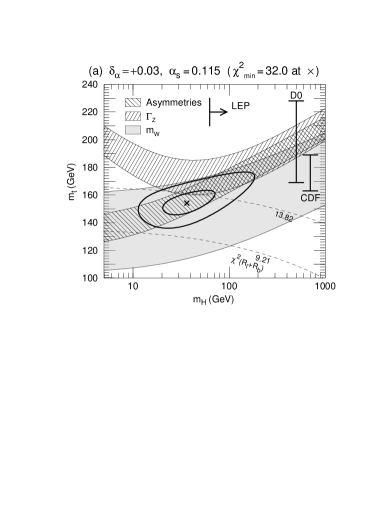
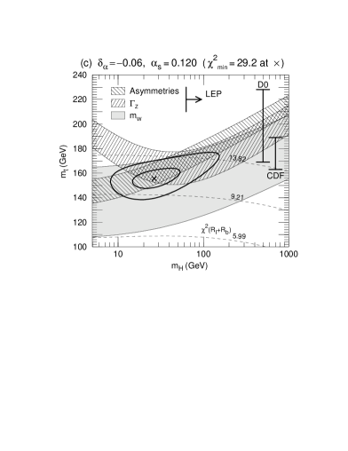
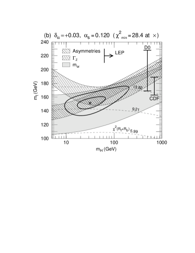
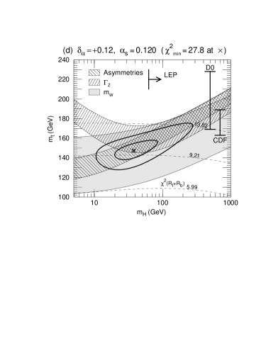
Figure 6: The SM fit to all electroweak data in the ($m_{H},\,m_{t}$) plane for (a) $(\delta_{\alpha},\alpha_{s})=(+0.03,0.115)$, (b) $(+0.03,0.120)$, (c) $(-0.06,0.120)$ and (d) $(+0.12,0.120)$. The thick inner and outer contours correspond to $\Delta\chi^{2}=1$ ($\sim$ 39%CL), and $\Delta\chi^{2}=4.61$ ($\sim$ 90%CL), respectively. The minimum of $\chi^{2}$ is marked by an “$\times$”, where the degree-of-freedom of the fit is 23. Also shown are the 1-$\sigma$ constraints from the $Z$-pole asymmetries, $\Gamma_{Z}$ and $m_{W}$. The dashed lines show the constraint from $R_{\ell}$ and $R_{b}$: $\chi^{2}\!=5.99,\,9.21,\,13.82$ correspond to 95%, 99%, 99.9%CL contours, respectively.

Quantities which help to disentangle the above $m_{t}$-$m_{H}$ correlation are $R_{\ell}$ and $R_{b}$. The constraints from these data are shown in Fig. 6 by dashed lines corresponding to $\chi^{2}=5.99$ (95%CL), $\chi^{2}=9.21$ (99%CL) and $\chi^{2}=13.82$ (99.9%CL) contours. These constraints can be clearly seen in Fig. 7 where we show the data and the SM predictions for $R_{\ell}$ and $R_{b}$. $R_{\ell}$ is sensitive to the assumed value of $\alpha_{s}$, and, for $\alpha_{s}=0.120$, the data favors smaller $m_{H}$. $R_{b}$ is, on the other hand, sensitive to neither $\alpha_{s}$ nor $m_{H}$, and the data strongly disfavors large $m_{t}$. It is thus the $R_{\ell}$ and $R_{b}$ data that constrain the values of $m_{t}$ and $m_{H}$ from above. If it were not for the data on $R_{\ell}$ and $R_{b}$ the common shaded region in Fig. 6

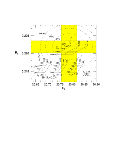
Figure 7: Constraints on the $R_{b}$ vs $R_{\ell}$ plane. The SM predictions are shown for $\alpha_{s}$=$0.11$, $0.12$, $0.13$ at $\delta_{\alpha}=0.03$. The ($\alpha_{s},\,\bar{\delta}_{b}$) lattice is obtained by allowing $\bar{\delta}_{b}$ to vary at $\bar{s}^{2}(m_{Z}^{2})=0.23039$.

with very large $m_{H}$ $(m_{H}\sim 1{\,\rm TeV})$ could not be excluded by the electroweak data alone.

It is clearly seen from Fig. 6 that the narrow “asymmetry” band is sensitive to $\delta_{\alpha}$, whereas the “$\Gamma_{Z}$” constraint is sensitive to $\alpha_{s}$. The fit improves at larger $\delta_{\alpha}$ (larger $1/\bar{\alpha}(m_{Z}^{2})$) because the “asymmetry” constraint then favors lower $m_{t}$ that is favored by the $R_{b}$ data. An update of the compact parametrization[5] of the $\chi^{2}_{\rm SM}$ function of the global fit has been reported in Ref.lp95_hag. For $m_{H}=60,300,1000{\,\rm GeV}$, $\alpha_{s}=0.120\pm 0.07$ and $\delta_{\alpha}=0.03\pm 0.09$, one obtains

$$m_{t}=179\pm 7{}^{+19(m_{H}=1000)}_{-22(m_{H}=60)}\mp 2(\alpha_{s})\mp 5(\delta_{\alpha})\,,$$ (22)

where the mean value is for $m_{H}=300$ GeV. The fit (22) agrees excellently with the estimate

$$m_{t}=180\pm 13~{}{\,\rm GeV}$$ (23)

from the direct production data at the Tevatron[28, 29]. Despite the claim[23] that there is no strong evidence for the genuine electroweak correction, which we re-confirmed above with the new data, this should be regarded as strong evidence that the standard electroweak gauge theory is valid at the quantum level. The accidental cancellation of the two large radiative effects in the observable combination $T^{\prime}$ of Eq.(8) tells us, in the face of the Tevatron results (23), the presence of the large electroweak correction to the muon-decay rate, $\bar{\delta}_{G}$, which is finite and calculable only in the gauge theory[30, 4].

Table 2: 95%CL upper and lower bounds of $m_{H}$(GeV) for a given $\alpha_{s}$ and $\delta_{\alpha}=0.03\pm 0.09$.

$\alpha_{s}$	all EW data			$-(R_{b},R_{c})$ data			$+m_{t}$ (Tevatron)
0.115		$16<m_{H}<150$			$18<m_{H}<290$			$22<m_{H}<360$
0.120		$13<m_{H}<180$			$15<m_{H}<500$			$20<m_{H}<550$
0.125		$11<m_{H}<220$			$12<m_{H}<1800$			$18<m_{H}<980$

As discussed above the constraint on $m_{H}$ from the electroweak data is sensitive to $R_{b}$, and hence to $\alpha_{s}$. Shown in Table 2 are the 95%CL upper and lower bounds on $m_{H}$(GeV) from the electroweak data. A low-mass Higgs boson is clearly favored. However, this trend disappears for $\alpha_{s}>0.12$ once we remove the $R_{b}$ and $R_{c}$ data. The present $m_{t}$ estimate (23) from the Tevatron does not significantly improve the situation.

It is instructive to anticipate the impact a precise measurement of the top-quark mass would have in the context of the present electroweak data. For instance, a precision measurement of $m_{t}$ with an error of 1 GeV is envisaged[31] at TeV33,

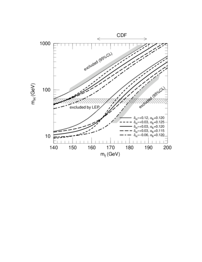
Figure 8: Constraints on the Higgs mass in the SM from all the electroweak data. Upper and lower bounds of the Higgs mass at 95%CL are shown as functions of the top mass $m_{t}$, where $m_{t}$ is treated as an external parameter with negligible uncertainty. The results are shown for $\alpha_{s}=0.120\pm 0.005$ and $\delta_{\alpha}\equiv 1/\bar{\alpha}(m_{Z}^{2})-128.72=0.03\pm 0.09$.

a proposed luminosity upgrade of the Tevatron. The 95%CL upper/lower bounds on $m_{H}$ from the electroweak data are shown in Fig. 8 as functions of $m_{t}$. Dependences of the bounds on the two remaining parameters, $\alpha_{s}=\alpha_{s}(m_{Z})_{\overline{\rm MS}}$ and $\delta_{\alpha}=1/\bar{\alpha}(m_{Z}^{2})-128.72$, are shown clearly. For a smaller value of $m_{t}$, $m_{t}<170$ GeV, a rather stringent upper bound on $m_{H}$ is obtained, whereas a medium-heavy Higgs boson is favored for $m_{t}>180$ GeV. It is tantalizing that the present data from the Tevatron (23) lies just on the boundary.

Fig. 8 shows us that once the top-quark mass is determined, either by direct measurements or by a theoretical model, the major remaining uncertainty is in $\delta_{\alpha}$, the magnitude of the QED running coupling constant at the $m_{Z}$ scale. It is clear[4] that we won’t be able to learn about $m_{H}$ in the SM, nor about physics beyond the SM from its quantum effects, without a significantly improved determination of $\bar{\alpha}(m_{Z}^{2})$.

3 The $R_{b}$ and $R_{c}$ Crisis and $\alpha_{s}$

The most striking results of the updated electroweak data are those of $R_{b}$ and $R_{c}$, which are shown in Fig. LABEL:fig:rbrc. The SM predictions to these ratios are shown by the thick solid line, where the top-quark mass in the $Zb_{L}b_{L}$ vertex correction is indicated by solid blobs. When combined the $R_{b}$ and $R_{c}$ data alone reject the SM at the 99.99%CL for $m_{t}>170$ GeV. The thin solid line represents the prediction of the extended SM where the $Zb_{L}b_{L}$ vertex function, $\bar{\delta}_{b}(m_{Z}^{2})$ of (2), is allowed to take an arbitrary value. In the SM the function $\bar{\delta}_{b}(m_{Z}^{2})$ always takes a negative value ($\bar{\delta}_{b}(m_{Z}^{2})\hbox to0.0pt{\lower 3.5pt\hbox{$\mathchar 0\relax\sim$}\hss}\raise 1.0pt\hbox{$<$}-0.03$), and its magnitude grows quadratically with $m_{t}$; see Eq.(16). The data are not only inconsistent with the SM but also inconsistent at more than the 2-$\sigma$ level with its extension where only the $Zb_{L}b_{L}$ vertex function is modified.

The correlation between the two observables, $R_{b}$ and $R_{c}$, can be understood as follows[2, 3]: To a good approximation, the measurement of $R_{c}$ does not depend on the assumed value of $R_{b}$, because it is measured by detecting leading charmed-hadrons in a leading-jet for which a b-quark jet rarely contributes. On the other hand, the measurement of $R_{b}$ is affected by the assumed value of $R_{c}$, since it typically makes use of its decay-in-flight vertex signal for which charmed particles can also contribute. We find that the following parametrization,

$$R_{b} = 0.2205-0.0136\frac{R_{c}-0.172}{0.172}\pm 0.0016,$$ (24a)

$$R_{c} = 0.1540\pm 0.0074,$$ (24b)

reproduces the results of Ref.lephf9502, as indicated by the shaded regions in Fig. LABEL:fig:rbrc.

Before discussing the implications of this striking result, we should recall the fact that the hadronic $Z$ partial width, $\Gamma_{h}$, is measured with 0.17% accuracy; see Eq.(• ‣ 2.2). This strongly constrains our attempt to modify theoretical predictions for the ratios $R_{b}$ and $R_{c}$. This is because $\Gamma_{h}$ can be approximately expressed as

$$\Gamma_{h} = \Gamma_{u}+\Gamma_{d}+\Gamma_{s}+\Gamma_{c}+\Gamma_{b}+\Gamma_{\rm others}$$ (25)

$$\sim \{\Gamma_{u}^{0}+\Gamma_{d}^{0}+\Gamma_{s}^{0}+\Gamma_{c}^{0}+\Gamma_{b}^{0}\}\times[1+\frac{\alpha_{s}}{\pi}+{\cal O}(\frac{\alpha_{s}}{\pi})^{2}],$$

where the $\Gamma_{q}^{0}$’s are the partial widths in the absence of the final state QCD corrections. Hence, to a good approximation, the ratios $R_{q}$ can be expressed as ratios of $\Gamma_{q}^{0}$ and their sum. A decrease in $R_{b}$ and an increase in $R_{c}$ should then imply a decrease and an increase of $\Gamma_{b}^{0}$ and $\Gamma_{c}^{0}$, respectively, from their SM predicted values. In order to satisfy the experimental constraint on $\Gamma_{h}$ one should hence adjust the $\alpha_{s}$ value in Eq.(25).

The consequence of this constraint is clearly shown in Fig. LABEL:fig:rbrc_vs_alphas where, once we allow both $\Gamma_{b}^{0}$ and $\Gamma_{c}^{0}$ to be freely fitted by the data, the above $\Gamma_{h}$ constraint forces $\alpha_{s}$ to be unacceptably large, $\alpha_{s}(m_{Z})=0.185\pm 0.041$. On the other hand, if we allow only $\Gamma_{b}^{0}$ to vary by assuming the SM value of $\Gamma_{c}^{0}$ (the straight line of the extended SM in Fig. LABEL:fig:rbrc), then the $\Gamma_{h}$ constraint gives a slightly small value, $\alpha_{s}(m_{Z})=0.104\pm 0.08$, which is compatible[5, 32] with some of the low-energy measurements[27, 33] and lattice QCD estimates[34, 35]. Although the SM does not reproduce the $R_{b}$ and $R_{c}$ data it gives a moderate $\alpha_{s}$ value consistent with the estimates based on the $e^{+}e^{-}$ jet-shape measurements[36, 37] and the hadronic $\tau$-decay rate[36].

In fact we do not yet have a definite clue where in the region $0.105<\alpha_{s}(m_{Z})<0.125$ the true QCD coupling constant lies. $\alpha_{s}\sim 0.12$ is favored from the electroweak data, if we believe in the SM predictions for $R_{b}$ and $R_{c}$ despite the strong experimental signals. On the other hand $\alpha_{s}\sim 0.11$ is favored if we believe in the SM predictions for $\Gamma_{c}^{0}$ while allowing new physics to modify $\Gamma_{b}^{0}$. These two solutions both lead to an acceptable $\alpha_{s}$ value at present. However, once we allow new physics in both $\Gamma_{b}^{0}$ and $\Gamma_{c}^{0}$ and let them be fitted by the data, then an unacceptably large $\alpha_{s}$ follows.

Even if we allow new-physics contributions for both $\Gamma_{b}^{0}$ and $\Gamma_{c}^{0}$, we cannot explain the discrepancies in $R_{b}$ and $R_{c}$ because of the constraint $0.105<\alpha_{s}(m_{Z})<0.125$. The only sensible solution, then, may be to allow new-physics contributions to all $\Gamma_{q}^{0}$ such that their sum stays roughly at the SM value, e.g. by making all the down-type-quark widths larger than their SM values by 3% and the up-type-quark widths to be smaller by 6%. Such a model would explain both $R_{b}$ and $R_{c}$, and give a reasonable $\alpha_{s}$. It is not easy to find a working model, however, which does not jeopardize all the excellent successes of the SM in the quark and lepton asymmetries, the leptonic widths, $m_{W}$, and in the low-energy neutral-current data.

The difficulty is exemplified in Figs. LABEL:fig:width_vs_beta and LABEL:fig:asym_vs_beta, where the effects of the $Z$-$Z^{\prime}$ mixing in the partial $Z$ widths and all the on-peak asymmetries are given for the models with an additional $Z$ boson in the ${\rm E_{6}}$ grand-unified theory. The additional $Z$ boson, $Z_{E}$, is a linear combination of the SU(5) singlet, $Z_{\chi}$, and the SO(10) singlet, $Z_{\psi}$, as

$$Z_{E}=Z_{\psi}\cos\beta+Z_{\chi}\sin\beta\,,$$ (26)

and the observed $Z$ boson, $Z_{1}$, is a mixture of the SM $Z$ boson, $Z_{\rm SM}$, and $Z_{E}$;

$$Z_{1}=Z_{\rm SM}\cos\theta_{E}+Z_{E}\sin\theta_{E}\,,$$ (27)

in the notation of Ref.hnst90. The models with $\beta\approx\pi$ can, for instance, make $R_{b}$ larger by 4% and $R_{c}$ smaller by 5%, while roughly keeping $\Gamma_{h}^{0}$, $\Gamma_{Z}^{0}$ and the on-peak asymmetries. However, these models should necessarily predict unacceptably large $\Gamma_{\ell}$ (by $\sim 6\%$) and too small $\Gamma_{\rm inv}$ (by $\sim 3\%$), in conflict with the severe constraints (• ‣ 2.2).

Because the $R_{c}$ measurement depends strongly on the charm-quark detection efficiency,  which has uncertainties in the charmed-quark fragmentation function into charmed hadrons and in charmed-hadron decay branching fractions, it is still possible that unexpected errors are hiding. As an extreme example, if as much as 10% of the charmed-quark final states were unaccounted for in the simulation program, then both the 10% deficit in $R_{c}$ at LEP and the 10% too few charmed hadron multiplicity in B-meson decays[38, 39] could be solved.

If we assume that $R_{c}$ actually has the SM value $R_{c}\sim 0.172$ and temporarily set aside its experimental constraint, then the correlation as depicted by Eq.(24a) tells that the measured $R_{b}=0.2205\pm 0.0016$ is about 2% larger than the SM prediction, $R_{b}\sim 0.216$ for $m_{t}\sim 175$ GeV. The discrepancy is still significant at the 3-$\sigma$ level.

I looked for the possibility that an experimental problem causing an underestimation of $R_{c}$ could lead to an overestimation of $R_{b}$. This turned out to be a difficult task, since $R_{b}$ is measured mainly by using a different technique, the double-tagging method[2, 3], where the $b$-quark tagging efficiency is determined experimentally rather than by estimating it from the $b$-quark fragmentation model and the $b$-flavored hadron decay rates. Schematically the single and double $b$-tag event rates ($N_{T}$ and $N_{TT}$, respectively) in hadronic two-jet events are expressed as

$$\frac{N_{T}}{2N_{h}} = \epsilon_{b}r_{b}R_{b}+\epsilon_{c}r_{c}R_{c}+\mbox{\rm others},$$ (28a)

$$\frac{N_{TT}}{N_{h}} = C\,\{\,\epsilon_{b}^{2}r_{b}R_{b}+\epsilon_{c}^{2}r_{c}R_{c}+\mbox{\rm others}\,\},$$ (28b)

where $\epsilon_{q}$ denotes the efficiency of tagging a $q$-jet, $r_{q}$ is the rate of two-jet-like events ($\mbox{\it Thrust}>0.8$) in the $q\bar{q}$ initiated events, and the deviation of $C$ from unity measures possible correlation effects between the two jets. By choosing the tagging condition such that $\epsilon_{b}\gg\epsilon_{c}$ one can self-consistently determine both $\epsilon_{b}$ and $R_{b}$:

$$R_{b}\,=\,\frac{C}{r_{b}}\,\frac{[\,\frac{N_{T}}{2N_{h}}-\epsilon_{c}\frac{r_{c}}{r_{b}}R_{c}-\cdot\cdot\cdot\,]^{2}}{[\,\frac{N_{TT}}{N_{h}}-\epsilon_{c}^{2}\frac{r_{c}}{r_{b}}R_{c}-\cdot\cdot\cdot\,]}\,.$$ (29)

In the limit of uncorrelated two-jet events only ($C=1$ and $r_{b}=1$), and in the limit of a negligible contribution from non-$b$ events ($\epsilon_{c}/\epsilon_{b}=0$), the ratio $R_{b}$ is determined from the ratio of the square of the single-tag event rate and the double-tag event rate. Only for the corrections to this limit are the QCD motivated hadron-jet simulation programs used. A compilation of very careful tests of these correction terms are found in the LEP/SLC Heavy Flavor Group report[2]. We should still examine if our present understanding of generating hadronic final states from quark-gluon states allows us to constrain the coefficients $C$ and $r_{b}$ at much less than one % level and the miss-tagging efficiency $\epsilon_{c}\sim 0.01$ at the 10% level. For instance, the combination of an overestimation of $C$ by 0.5% with an underestimation of $r_{b}$ by 0.5% and that of $\epsilon_{c}$ by 10%, can result in an overestimate of $R_{b}$ by 2%. Serious theoretical studies of the uncertainty in the present hadron-jet generation program are needed, because in my opinion, these programs have never been tested at the accuracy level that was achieved by these excellent experiments at LEP.

4 Attempts to Explain Large $R_{b}$

There have been many attempts to explain the discrepancy in $R_{b}$ by invoking new physics beyond the SM. Most notably, in the minimal supersymmetric (SUSY) SM[40, 41, 42, 43, 44, 45, 46, 47, 48, 49, 50, 51, 52, 53], an additional loop of a light $\tilde{t}_{R}$ and a light higgsino-like chargino, or that with an additional Higgs pseudoscalar when $\tan\beta\gg 1$, can compensate the large negative top-quark contribution of the SM in the $Zb_{L}b_{L}$ vertex function. Such a solution typically leads to the prediction that the masses of the lighter $\tilde{t}$ and chargino, or the pseudoscalar should be smaller than $m_{Z}$. In the former scenario the top quark should have significant exotic decays into $\tilde{t}_{R}$ and a neutral Higgsino, and in the latter scenario another exotic decay, $t\rightarrow b+H^{+}$, may occur[47, 50, 51, 52, 53]. In both SUSY scenarios we should expect to find new particles at the Tevatron, LEP2 or even at LEP1.5.

It is worth remarking here that the small $\alpha_{s}$ value which is obtained by allowing

Figure 13: Constraints on $\alpha_{s}(m_{Z})_{\overline{\rm MS}}$ as functions of the SUSY threshold scale $m_{\rm SUSY}$ in the minimal SUSY-SU(5) model and in the model with the missing-doublet mechanism.

a new physics contribution to explain the $R_{b}$ anomaly tends to destroy the SUSY-SU(5) unification of the three gauge couplings in the minimal model[54]. This problem is, however, highly dependent on details of the particle mass spectrum at the GUT scale. In fact in the missing-doublet[55] SUSY-SU(5) model which naturally explains the doublet-triplet splitting, smaller $\alpha_{s}$ is prefered due to its peculiar GUT particle spectrum[56, 57, 58]. I show in Fig. 13 the update for the allowed regions of $\alpha_{s}(m_{Z})$ in the two SUSY-SU(5) models as functions of the heavy Higgsino mass, where the standard supergravity model assumptions are made for the SUSY particle masses at the electroweak scale[22].

In an alternative scenario of electroweak symmetry breaking, the Techni-Color (TC) model, the heavy top-quark mass implies strong interactions among top-quarks and techniquarks. Such interactions, typically called the extended technicolor (ETC) interactions, can affect the $Zb_{L}b_{L}$ vertex: see Fig. 14. However, the side-ways ETC bosons that connect the top-quark and techniquark leads to a contribution with an opposite sign[59, 60]. The diagonal ETC bosons contribute[61] with the correct sign[62], and their phenomenological consequences have been studied[63, 64]. Although the diagonal ETC bosons can explain the $R_{b}$ data[64], it has been pointed out[65] that such models should necessarily give an unacceptably large contribution to either the $S$ or the $T$ parameter. See Ref.kitazawa95 for more discussions on these models.

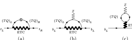
Figure 14: The side-ways ETC (Extended Techni-Color) bosons contribute to both (a) the top-quark mass and (b) the $Zb_{L}b_{L}$ vertex. (c) Diagonal ETC bosons can also contribute to the $Zb_{L}b_{L}$ vertex.

As an alternative to the standard ETC model where the ETC gauge group commutes with the SM gauge group, models with a non-commuting ETC gauge group have been proposed[67] which have rich phenomenological consequences[68].

So far, the above models affect mainly the $Zb_{L}b_{L}$ coupling, which dominates the $Zb_{R}b_{R}$ coupling in the SM. A possible anomaly in the $b$-jet asymmetry parameter, $A_{b}$, observed at the SLC with its polarized beam (see Fig. 1) may suggest a new physics contribution in the $Zb_{R}b_{R}$ vertex[69]. It is worth watching improved $A_{b}$ measurements at the SLC in the near future.

It has also been proposed[70] that a new heavy gauge boson $X$ which couples only to the third-generation quarks and leptons may affect the $Z$ boson experiments through its mixing with the SM $Z$. Such models affect not only the $Zbb$ vertex but also the $Z\tau\tau$ and $Z\nu_{\tau}\nu_{\tau}$ vertices. The original proposal[70] with the axial-vector $Xbb$ coupling and the vector $X\tau\tau$ coupling should be re-examined in view of the $e$-$\mu$-$\tau$ universality of the 1995 data, Eq.(• ‣ 2.2), and the possible anomaly in $A_{b}$.

5 Quark-Lepton Universality Violation in Charged Currents

The tree-level universality of the charged-current weak interactions is one of the important consequences of the ${\rm SU(2)_{L}}$ gauge symmetry. The universality between quark- and lepton-couplings is expressed as the unitarity of the Cabibbo-Kobayashi-Maskawa (CKM) matrix. After correcting for the SM radiative corrections, the present experimental data[71, 72] gives

$$|V_{ud}|^{2}+|V_{us}|^{2}+|V_{ub}|^{2}-1=-0.0017\pm 0.0015\,.$$ (30)

Figure 15: The 1-$\sigma$ allowed region in the ($m_{\tilde{C}_{1}}$, $m_{\tilde{\nu}}$) plane from the universality violation (30).

Universality is violated at the 1-$\sigma$ level.

Here again, the most important observation is that the quark-lepton universality of the $W$ couplings is verified experimentally at the 0.2% level. This excellent agreement is found only after the SM radiative corrections are applied[72]. Eq.(30) therefore strongly constrains any new interactions which distinguish between quarks and leptons.

It turned out that the 0.1% level of the non-universality is expected in the MSSM, where the expected mass differences between squarks and sleptons can naturally lead to the quark-lepton non-universality at the one-loop level[73, 74, 75]. The effect, however, disappears quickly if the relevant SUSY particle masses are much bigger than $m_{Z}$.

Shown in Fig. 15 is the 1-$\sigma$ allowed region of masses of the sneutrino $\tilde{\nu}$ and the lighter chargino, $\tilde{C}_{1}$, in the MSSM. The ratio of the two vacuum expectation values is set at $\tan\beta=(1,2,10)$. The 1-$\sigma$ upper bounds are roughly $m_{{\tilde{\nu}}}<220$ GeV and $m_{\tilde{C}_{1}}<600$ GeV, respectively. It has been found[75] that the sign and the magnitude of the quark-lepton universality violation (30) favor light sleptons and relatively light chargino and neutralinos with significant gaugino components. Details are found in Refs.hmy95,yhm95.

6 Conclusions

The most important hint of physics beyond the Standard Model (SM) from the 1995 precision electroweak data is that the most precisely measured quantities, the total, leptonic and hadronic decay widths of the $Z$ and the effective weak mixing angle, $\sin^{2}\theta_{W}$, measured at LEP and SLC, and the quark-lepton universality of the weak charged currents measured at low energies, all agree with the predictions of the SM at a few $\times 10^{-3}$ level. Any attempts to replace the SM by a more fundamental theory should hence explain why quantum effects from new physics are tiny for these quantities.

A most natural explanation seems to me that the new physics beyond the SM is essentially weakly interacting, and its quantum effects decouple. The supersymmetric (SUSY) SM is a good example of such a model.

On the other hand, if new physics has a strongly interacting sector one may need a mechanism that naturally hides its potentially large quantum effects. The technicolor (TC) scenario of the dynamical electroweak symmetry breaking belongs to this class, but I do not know of a mechanism that naturally kills all additional quantum corrections.

In this report I examined implications of the three possible discrepancies between experiments and the SM predictions. They are the 11% (2.5-$\sigma$) deficit of the $Z$-partial-width ratio $R_{c}=\Gamma_{c}/\Gamma_{h}$, the 2% (3-$\sigma$) excess of the ratio $R_{b}=\Gamma_{b}/\Gamma_{h}$, and the 0.17% (1-$\sigma$) deficit of the CKM unitarity relation $|V_{ud}|^{2}+|V_{us}|^{2}+|V_{ub}|^{2}=1$.

I first explained in detail the difficulty in interpreting the present $R_{c}$ data. Because the $Z$ hadronic width, $\Gamma_{h}$, agrees with the SM prediction at the 0.2% level, the 11% deficit in $R_{c}$ should necessarily lead to an unacceptably large $\alpha_{s}$ if the other hadronic widths of the $Z$ boson remain unaffected. An acceptable value of $\alpha_{s}$ is obtained only if the deficit in $\Gamma_{c}$ is compensated rather accurately by an excess in the rest of the hadronic widths $\Gamma_{u}+\Gamma_{d}+\Gamma_{s}+\Gamma_{b}$. In addition, we must reproduce all the quark and lepton asymmetry data, the leptonic widths and the other successful predictions of the SM. I was unable to find such a solution.

If we assume the SM value for $R_{c}$, then we should identify the cause of an over-estimation in its experimental determination. It is possible that such an over-estimation occurs through several systematic errors in the input parameters that determine the detection efficiency of the primary charm-quark events commonly adopted by all experiments at LEP. The $R_{b}$ data may, nevertheless, be taken seriously, since they are obtained by using the double tagging technique that allows us to measure the $b$-quark-jet tagging efficiency. It is not clear to me, however, if our understanding of hadron-jet formation is good enough to establish the 2% excess in $R_{b}$ at the 3-$\sigma$ level.

If we take the present $R_{b}$ data, it gives us a 3-$\sigma$ evidence for physics beyond the SM. It may either signal a relatively large additional quantum correction or a new tree-level neutral-gauge-boson interaction that couples to $b$. In the former case, the large radiative effect may either come from the large Yukawa coupling in the SUSY-SM or the new strong interaction that makes the top-quark massive in the Technicolor (TC) scenario of the electroweak gauge symmetry breaking. In the SUSY-SM, one is forced to have either a combination of a very light $\tilde{t}_{R}$ and Higgsino or that of the large $b$-quark Yukawa coupling and a very light Higgs boson. In either case, one expects to observe new particles at LEP2 or in the top-quark decay at the Tevatron. It is worth noting that these SUSY scenarios do not cause any difficulty in the other sector of precision electroweak physics. In the TC scenario, one typically obtains large radiative effects to the $Zb_{L}b_{L}$ vertex from the ETC-gauge-boson interactions that give rise to the top-quark mass. The side-ways-boson exchange contributes with the wrong sign, while the diagonal-boson exchange contributes with the correct sign. The naive ETC models, however, suffer from either too large an $S$ for models with custodial SU(2) symmetry or too large a $T$ for models without custodial SU(2). Models with the ETC gauge group that contains the electroweak ${\rm SU(2)_{L}}$ might evade such immediate difficulty.

Finally, I examined consequences of the possible violation of quark-lepton universality in low-energy charged-current interactions. Although the observed deficit in the CKM unitarity relation is only 0.17% at the 1-$\sigma$ level, we showed that this is what the minimal SUSY-SM predicts if sleptons and gauginos are sufficiently light.

In conclusion, none of the above three hints of deviations from the SM predictions are convincing to me. The first two data, $R_{c}$ and $R_{b}$, are experimentally significant but they do not lead us to a satisfactory picture of physics beyond the SM, yet. The last example, the SUSY-SM explanation of the violation of the CKM unitarity relation, can naturally co-exist with all the other excellent successes of the SM, but its experimental significance is marginal.

I feel strongly that the experimental accuracy of the precision electroweak measurements has finally reached the level where new physics can be probed via its quantum effects. The $R_{b}$ data, if even more firmly established, would pose a serious challenge to theorists. Intimate and attentive cooperation between experimentalists and theorists is needed more than ever.

References

- [1] The LEP Electroweak Working Group, Internal Note LEPEWWG/95-02.
- [2] The LEP Electroweak Heavy Flavours Working Group, Internal Note LEPHF/95-02.
- [3] P.B. Renton, Talk at XVII International Symposium on Lepton and Photon Interactions at High Energies , 10–15 Aug 1995, Beijing, China.
- [4] K. Hagiwara, Talk at XVII International Symposium on Lepton and Photon Interactions at High Energies , 10–15 Aug 1995, Beijing, China (KEK-TH-461, hep-ph/9512425).
- [5] K. Hagiwara, D. Haidt, C.S. Kim and S. Matsumoto, Z. Phys. C64 (1994) 559; C68 (1995) 352(E); S. Matsumoto, Mod. Phys. Lett. A10 (1995) 2553.
- [6] M.E. Peskin and T. Takeuchi, Phys. Rev. Lett. 65 (1990) 964; Phys. Rev. D46 (1992) 381.
-
[7]
J.M. Cornwall and J. Papavassiliou,
Phys. Rev. D40 (1989) 3474;
J. Papavassiliou and K. Phillippides, ibid.48(1993)4225; ibid.51(1995)6364;
J. Papavassiliou, ibid.50(1994)5998. - [8] G. Degrassi and A. Sirlin, Nucl. Phys. B383 (1992) 73; Phys. Rev. D46 (1992) 3104; G. Degrassi, B. Kniehl and A. Sirlin, ibid.48(1993)R3963.
- [9] D.C. Kennedy and B.W. Lynn, Nucl. Phys. B322 (1989) 1.
- [10] K. Hagiwara, S. Matsumoto and R. Szalapski, Phys. Lett. B357 (1995) 411.
- [11] A. Sirlin, Phys. Rev. D22 (1980) 971.
- [12] K. Hagiwara, S. Ishihara, R. Szalapski and D. Zeppenfeld, Phys. Rev. D48 (1993) 2182.
- [13] A.D. Martin and D. Zeppenfeld, Phys. Lett. B345 (1995) 558.
- [14] M.L. Swartz, Preprint SLAC-PUB-95-7001, hep-ph/9509248.
- [15] S. Eidelman and F. Jegerlehner, Z. Phys. C67 (1995) 602.
- [16] H. Burkhardt and B. Pietrzyk, Phys. Lett. B356 (1995) 398.
- [17] B.A. Kniehl, Nucl. Phys. B347 (1990) 86.
- [18] T. Takeuchi, Talk at Yukawa International Seminar, Kyoto, Japan, 20–25 Aug 1995.
- [19] K. Hagiwara, D. Haidt and S. Matsumoto, to be published.
- [20] K. McFarland, Talk at XV Workshop on Weak Interactions and Neutrinos, Talloires, France, 4–8 Sep 1995.
- [21] T. Appelquist and J. Terning, Phys. Lett. B315 (1993) 139; Phys. Rev. D50 (1994) 2116.
- [22] K. Hagiwara, S. Matsumoto and Y. Yamada, in preparation.
- [23] V.A. Novikov, L.B. Okun and M.I. Vysotsky, Mod. Phys. Lett. A8 (1993) 2529; Erratum A8(1993)3301.
- [24] G.L. Fogli and D. Haidt, Z. Phys. C40 (1988) 379.
- [25] P. Langacker, in Precision Tests of the Standard Electroweak Model, ed. by P. Langacker (World Scientific, 1994).
- [26] K. Hagiwara, R. Najima, M. Sakuda and N. Terunuma, Phys. Rev. D41 (1990) 815.
- [27] Particle Data Group, L. Montanet et al., Phys. Rev. D50 (1994) 1173.
- [28] CDF Collaboration, F. Abe et al., Phys. Rev. Lett. 74 (1995) 2626.
- [29] D0 Collaboration, S. Abachi et al., Phys. Rev. Lett. 74 (1995) 2632.
- [30] P.Gambio and A.Sirlin, Phys. Rev. Lett. 73 (1994) 621.
- [31] D. Amidei et al., Preprint CDF/DOC/TOP/PUBLIC/3265 (Aug 1995).
- [32] M. Shifman, Mod. Phys. Lett. A10 (1995) 605. 20
- [33] D. Harris, CCFR collab., Talk at XXX’th Recontre de Moriond, Les Arcs, France, March 19–26, 1995.
- [34] A.X. El-Khadra et al., Phys. Rev. Lett. 69 (1992) 729.
- [35] C.T.H. Davieset al., Phys. Rev. D50 (1994) 6963; Phys. Lett. B345 (1995) 42.
- [36] S. Bethke, Talk at XXX’th Recontre de Moriond, 19–25 Mar 1995, Les Arcs, France.
- [37] K. Baird, SLD collab., Talk at XXX’th Recontre de Moriond, 19–25 Mar 1995, Les Arcs, France.
- [38] G. Buchalla, I. Dunietz and H. Yamamoto, FERMILAB-PUB-95-167-T, hep-ph/9507437.
- [39] M. Neubert, Talk at XVII International Symposium on Lepton and Photon Interactions at High Energies , 10–15 Aug 1995, Beijing, China.
- [40] M. Boulware and D. Finnell, Phys. Rev. D44 (1991) 2054.
- [41] G. Altarelli, R. Barbieri and F. Caravaglios, Phys. Lett. B314 (1993) 357.
- [42] J.D. Wells, C. Kolda and G.L. Kane, Phys. Lett. B338 (1994) 219.
- [43] J.E. Kim and G.T. Park, Phys. Rev. D50 (1994) 6686; D51 (1995) 2444.
- [44] D. Garcia, R.A. Jiménez and J. Solà, Phys. Lett. B347 (1995) 309; 321; B351 (1995) 602(E).
- [45] D. Garcia, J. Solà, Phys. Lett. B354 (1995) 335; B357 (1995) 349.
- [46] A. Dabelstein, W. Hollik and W. Mösle, Talk at Ringberg Workshop on “Perspectives for electroweak interactions in collisions”, February 1995, hep-ph/9506251.
- [47] G.L. Kane, R.G. Stuart and J.D. Wells, Phys. Lett. B354 (1995) 350.
- [48] P.H. Chankowski and S. Pokorski, Phys. Lett. B356 (1995) 307.
- [49] M. Carena and C.E.M. Wagner, Nucl. Phys. B452 (1995) 45; C.E.M. Wagner, talk at SUSY95, Palaiseau, France, May 1995, hep-ph/9510341.
- [50] X. Wang, J.L. Lopez and D.V. Nanopoulos, Phys. Rev. D52 (1995) 4116.
- [51] E. Ma and D. Ng, Preprint TRI-PP-95-55, hep-ph/9508338.
- [52] J.D. Wells and G.L. Kane, Preprint SLAC-PUB-95-7038, hep-ph/9510372.
- [53] Y. Yamada, K. Hagiwara and S. Matsumoto, Talk by Y. Yamada at Yukawa International Seminar, Kyoto, Japan, 20–25 Aug 1995, hep-ph/9512227.
-
[54]
S. Dimopoulos and H. Georgi,
Nucl. Phys. B193 (1981) 150;
N. Sakai, Z. Phys. C11 (1981) 153. - [55] A. Masiero, D.V. Nanopoulos, K. Tamvakis, and T. Yanagida, Phys. Lett. 115B (1982) 380.
-
[56]
K. Hagiwara and Y. Yamada, Phys. Rev. Lett. 70 (1992) 709;
Y. Yamada, Z. Phys. C60 (1993) 83. - [57] J. Bagger, K. Matchev and D. Pierce, Phys. Lett. B348 (1995) 443.
- [58] J.L. Lopez and D.V. Nanopoulos, CTP-TAMU-29-95, hep-ph/9508253.
- [59] R.S. Chivukula, S.B. Selipsky, and E.H. Simmons, Phys. Rev. Lett. 69 (1992) 575; R.S. Chivukula, E. Gates, E.H. Simmons, and J. Terning, Phys. Lett. B311 (1993) 157.
- [60] N. Evans, Phys. Lett. B331 (1994) 378.
- [61] N. Kitazawa, Phys. Lett. B313 (1993) 395.
- [62] G.-H. Wu, Phys. Rev. Lett. 74 (1995) 4137.
- [63] C-X. Yue, Y-P. Kuang, G-R. Lu and L-D. Wan, Phys. Rev. D52 (1995) 5314.
- [64] K. Hagiwara and N. Kitazawa, Phys. Rev. D52 (1995) 5374.
- [65] T. Yoshikawa, Preprint HUPD-9514 (1995), hep-ph/9506411; Talk at Yukawa International Seminar, Kyoto, Japan, 20–25 Aug 1995.
- [66] N. Kitazawa, Talk at Yukawa International Seminar, Kyoto, Japan, 20–25 Aug 1995, hep-ph/9510334; N. Kitazawa and T. Yanagida, Preprint TMUP-HEP-9505, hep-ph/9510228; Preprint TMUP-HEP-9509, hep-ph/9511364.
- [67] R.S. Chivukula, E.H. Simmons and J. Terning, Phys. Lett. B331 (1994) 383; Preprint BUHEP-95-19, hep-ph/9506427.
- [68] E.H. Simmons, R.S. Chivukula and J. Terning, Talk by E.H. Simmons at Yukawa International Seminar, Kyoto, Japan, 20–25 Aug 1995, hep-ph/9509392.
- [69] M. Peskin, Comment at Yukawa International Seminar, Kyoto, Japan, 20–25 Aug 1995.
- [70] B. Holdom, Phys. Lett. B339 (1994) 114; ibid.351 (1995) 279.
- [71] I.S. Towner, Phys. Lett. B333 (1994) 13.
- [72] A. Sirlin, talk at Ringberg Workshop on “Perspectives for Electroweak Interactions in Collisions”, February 1995, hep-ph/9504385.
- [73] R. Barbieri, C. Bouchiat, A. Georges and P. Le Doussal, Phys. Lett. 156B (1985) 348; Nucl. Phys. B269 (1986) 253.
- [74] R. Barbieri, M. Frigeni and F. Caravaglios, Phys. Lett. B279 (1992) 169.
- [75] K. Hagiwara, S. Matsumoto and Y. Yamada, Phys. Rev. Lett. 75 (1995) 3605.