MIT-CTP-2501

hep-ph/9512439

Supernatural Inflation: Inflation from Supersymmetry with No (Very) Small Parameters

Lisa Randall

Marin Soljačić

Alan H. Guth

Laboratory for Nuclear Science and Department of Physics
Massachusettts Institute of Technology
Cambridge, MA 02139

Abstract

Most models of inflation have small parameters, either to guarantee sufficient inflation or the correct magnitude of the density perturbations. In this paper we show that, in supersymmetric theories with weak scale supersymmetry breaking, one can construct viable inflationary models in which the requisite parameters appear naturally in the form of the ratio of mass scales that are already present in the theory. Successful inflationary models can be constructed from the flat-direction fields of a renormalizable supersymmetric potential, and such models can be realized even in the context of a simple GUT extension of the MSSM. We evade naive “naturalness” arguments by allowing for more than one field to be relevant to inflation, as in “hybrid inflation” models, and we argue that this is the most natural possibility if inflaton fields are to be associated with flat direction fields of a supersymmetric theory. Such models predict a very low Hubble constant during inflation, of order $10^{3}$-$10^{4}$ GeV, a scalar density perturbation index $n$ which is very close to or greater than unity, and negligible tensor perturbations. In addition, these models lead to a large spike in the density perturbation spectrum at short wavelengths.

I Introduction

Inflationary models [1] in general require small parameters in the particle theory Lagrangian, to provide the flat potential needed for sufficient inflation and for the correct magnitude of density fluctuations. The need for unmotivated small parameters tends to weaken the credibility of a theory, so one hopes that the origin of these parameters can be understood. It is conceivable, of course, that the explanation lies beyond our present understanding, just as we presently have no accepted explanation of why the Yukawa coupling of the electron is $2\times 10^{-6}$, or why the weak scale lies 17 orders of magnitude below the Planck scale. Nonetheless, it would be encouraging to find that the small parameters required by inflation could be obtained from small parameters that are already essential to the particle theory, so that no additional small parameters are introduced. Models in which the small parameters arise as ratios of known particle physics mass scales are particularly attractive [2].

From a field theoretical perspective, it is difficult to see how flat direction fields can be present in a nonsupersymmetric theory (with the exception of Goldstone bosons, considered in Ref. [3]) given the effect of radiative corrections . We will assume therefore that the world is supersymmetric, and ask whether an inflationary potential can arise naturally in the context of the mass scales which we expect might be present. Some natural candidates for these scales could be the Planck scale $M_{p}\approx 10^{19}$ GeV, the GUT scale $M_{\rm G}\approx 10^{16}$ GeV, the intermediate scale $M_{I}\approx 10^{11}$ GeV, and the supersymmetry breaking scale $m_{3/2}\approx 1$ TeV.

However, straightforward considerations show that it is difficult to implement this strategy. The magnitude of density perturbations points to the GUT scale as setting the energy density during inflation, since $(M_{\rm GUT}/M_{p})^{2}\sim 10^{-6}$. Although suggestive, it is difficult to exploit this high scale in an inflationary model. In Ref. [4] it was argued that the necessity for cancelling the cosmological constant after inflation provides significant restrictions on a model in which the inflation scale is greater than the supersymmetry breaking scale. Models have been suggested in which the energy density in the early universe is well above the low energy supersymmetry breaking scale, and might be governed for example by the value of a moduli field [5, 6]. For these models, it must be checked that the constraint of Ref. [4] is satisfied. Beyond this, however, it is difficult to study such models in detail without a concrete realization.

It might also be that the inflation scale is generated by GUT physics. An interesting example of this type of model is Ref. [7]. It is however questionable whether the GUT scale exists as a fundamental scale of particle physics at all in light of the doublet-triplet splitting problem [8]. Furthermore, it is likely that the inflaton field would be charged under the GUT group and the reheat temperature would be too high (in excess of the gravitino bound).

In the context of supersymmetric models, an attractive scale for the vacuum energy density during inflation would be set by the intermediate scale, $M_{I}$. This scale is very likely to be present in a hidden sector model of supersymmetry breaking. It is also the right energy scale for the potential associated with moduli fields, which might be natural candidates for flat directions. The problem here, however, is that simple dimensional analysis arguments (to be reviewed in Sec. 2) show that density perturbations would generically be either far too small [9, 4] or far too large, depending on assumptions. For the case of inflation driven by a single moduli field, the dimensional arguments show that the requirements of sufficient inflation and correct density perturbations imply that 1) the variation of the inflaton (moduli) field during inflation is of order $M_{p}$, and 2) the energy density during inflation is of order $M^{4}$ where $M\approx 10^{16}$ GeV. An energy density of order $M_{I}^{4}$ would produce density perturbations too small by about ten orders of magnitude. For the case of a chaotic inflationary scenario, the variation of the inflaton is again of order $M_{p}$, but in this case the density perturbations are much too large unless the quartic coupling $\lambda$ is about $10^{-12}$.

In this paper, we show that the argument that inflation at an intermediate scale is untenable lacks sufficient generality, and can evaporate if one drops the assumption that inflation is driven by a single scalar field. We describe a class of two-field models, for which dimensional analysis estimates show that 1) the variation of the inflaton is of order $M_{I}$ or less, and 2) the energy density during inflation is of order $M_{I}^{4}$. We then go on to illustrate these ideas with models motivated by supersymmetry with soft supersymmetry breaking. We will find that these models not only solve the naturalness problem of obtaining sufficiently many e-foldings of inflation, but also generate very nearly the correct size of density perturbations based on the parameters of supersymmetry breaking. We therefore refer to our models as “supernatural” inflation.

This model contains a similar structure to the “hybrid” inflation models, proposed by Linde and studied by Copeland, Liddle, Lyth, Stewart, and Wands [10]. The fact that the standard dimensional naturalness arguments for the number of $e$-foldings and for $\delta\rho/\rho$ do not apply, and that the Hubble scale during inflation will be low was also clearly recognized by these authors. Our point here is to emphasize that the most natural scales for successful implementation of two field inflation of the “waterfall” type are the scales associated with supersymmetry breaking and the Planck scale. Furthermore, our models more accurately reflect masses and couplings associated with flat direction fields, and we will motivate the parameters and potential we use by consideration of flat directions in the MSSM. Hybrid inflation in the context of SUSY leads one to the interesting conclusion that the Hubble scale during the inflation which established the density perturbations might have been of order $10^{3}$–$10^{4}$ GeV, rather than $10^{13}$ GeV.

In the following section, we present the general arguments for why supersymmetry scales do not work in single field inflation models. We then review the general idea of “hybrid” or “waterfall” [10] models, and show why the single-field arguments do not apply to the two-field case. In Section 3, we present supernatural inflation models, in which we assume the inflation sector consists of flat direction fields whose potential is generated through supersymmetry breaking and nonrenormalizable operators. We derive the constraints on parameters consistent with the requisite number of $e$-foldings and density perturbations. In Section 4 we explore the possibility of a renormalizable coupling between the flat direction fields. In the following section we motivate the models of Sections 3 and 4 by briefly considering flat direction fields in the standard model, and present an illustration of the model of Section 4 in the context of a GUT extension of the MSSM. In Section 6, we give details of the evolution of the two fields in our models. We analyze the density perturbations that result from this evolution, and discover a novel spike that is predicted to appear at short wavelengths. Such a spike could lead to overproduction of black holes, but we show in Section 7 that existing constraints on black holes are satisfied for the parameters of interest. In Section 8, we show that the thermal production of gravitinos is also not a problem in our models. In the following section we show that successful baryogenesis can be accomplished in the context of late inflation. In Section 9, we discuss miscellaneous aspects of our models, and in Section 10, we conclude.

II One vs. Two Field Inflation

We begin this section by reviewing the “standard” arguments for why the inflaton in “natural” inflationary models varies on the scale $M_{p}$ and why the scale for the energy density should be larger than the intermediate scale in inflationary models with a single field.

For the purposes of these dimensional arguments, we first assume the potential takes the form

$${\cal V}=M^{4}{\cal G}(\phi/f)$$ (1)

where ${\cal G}$ is a bounded function of order unity. Here we have in mind for example a moduli field, with $M\approx M_{I}$. If we assume the slow roll equation of motion $3H\dot{\phi}=-{\cal V^{\prime}}$, where $H$ is the Hubble constant during inflation, the number of $e$-foldings is

$$N=\int Hdt=\int d\phi{H\over\dot{\phi}}=-\int d\phi{{\cal V}\over M_{p}^{2}{\cal V^{\prime}}}\approx-{\Delta\phi\over M_{p}}{f\over M_{p}}{{\cal G}\over{\cal G^{\prime}}}$$ (2)

There are essentially two possibilities. If ${\cal G}$ is a bounded function, and ${\cal G^{\prime}}$ is not very tuned to have very flat sections, one is in the regime of what might be expected for a moduli type field. In this case, the requirement of about 60 $e$-foldings of inflation favors $f$ of order $M_{p}$ and a change in $\phi$ during inflation at least of order $M_{p}$. Even when this is satisfied, some tuning of the potential is required.

The alternative possibility is that one is in a chaotic [11] inflationary scenario, in which case ${\cal G}$ will be dominated by monomial behavior for sufficiently large field, and ${\cal V^{\prime}}\approx{\cal V}/\phi$. In this case, $f$ is not defined, but one would still conclude $\Delta\phi\approx M_{p}$.

Density fluctuations are also readily estimated under the assumed form of the potential. They are given by

$${\delta\rho\over\rho}\approx{H^{2}\over\dot{\phi}}\approx{H^{3}\over{\cal V^{\prime}}}\approx\left({M\over M_{p}}\right)^{2}{f\over M_{p}}{{\cal G}^{3/2}\over{\cal G^{\prime}}}$$ (3)

Assuming a potential of the moduli type, with ${\cal G}$ and ${\cal G^{\prime}}$ of order unity and $f$ of order $M_{p}$, we find that ${\delta\rho\over\rho}\approx\left({M\over M_{p}}\right)^{2}$ favoring $M\approx 10^{-3}M_{p}$. Detailed calculations might change $M$ by an order of magnitude or so, but it is clear that $M\approx 10^{11}{\rm\ GeV}\approx M_{I}$ is strongly disfavored.

In a chaotic scenario on the other hand, one would conclude that the density fluctuations are too large unless there is a small parameter. For example, a simple dimensional argument would lead to the conclusion that for $V=\lambda\phi^{4}$, $\lambda\approx 10^{-12}$. Without further motivation for these small numbers, such a potential seems unlikely.

So one is led to the conclusion that it is difficult to naturally obtain sufficiently many e-foldings and the correct magnitude of density perturbations, without invoking either small numbers or a new mass scale.

It is apparent, however, that there is a loophole in the above argument. From Eq. (2) it is clear that the constraints on $f$ and $\Delta\phi$ during inflation arise because it is the same potential ${\cal V}(\phi)$ that controls the inflation rate $H$ and the speed of the inflaton field $\dot{\phi}$. These constraints can be avoided, therefore, if the energy density during inflation is provided from some source other than the scalar field which rolls and controls the ending of inflation.

The simplest way to implement this idea would be with two fields. This idea is essentially that first proposed by Linde [10] as “hybrid” inflation or “waterfall” models. There are two fields $\psi$ and $\phi$. The first field, which we call the inflaton, has a very flat potential. It starts at a large field value, and slowly rolls (via its classical field equations) to the origin.

The second field, $\phi$, has a potential whose minimum is far from the origin. In most previous incarnations of hybrid inflation, the scale of variation of this field is $M_{I}$, though in our models the scale will be $M_{p}$. When $\psi$ has large field value, it gives a positive mass squared term in the $\phi$ potential at the origin, so the classical field equations push $\phi$ to the origin. When $\psi$ gets sufficiently small (of order $M_{I}$ or less in our models), the mass squared of $\phi$ goes negative, and $\phi$ makes the transition from the origin to $M_{p}$.

The key feature of this model is that the energy density during inflation is dominated by the potential energy of the $\phi$ field at $\phi=0$. There are no tunings in the $\psi$ potential to get a small mass during inflation and a large mass afterwards, since its mass is always small, as is its potential energy. Because $H$ depends on the value of $\phi$ and is not determined by the field $\psi$, which acts as a switch to end inflation, the naive estimates do not apply.

The second key feature of this model is that the ending of inflation is controlled by when the $\phi$ mass squared at the origin changes sign. One can obtain a large number of $e$-foldings with the variation of the inflaton field $\psi$ much less than $M_{p}$. Let us see this explicitly.

We assume a potential which takes the form

$${\cal V}=M^{4}{\cal G}(|\phi|/f)+g(|\phi|,|\psi|)+m^{2}|\psi|^{2}$$ (4)

where $M$ and $f$ are to be determined, the function $g$ is the term responsible for the $\psi$ dependence of the $\phi$ mass, and $m$ is of order $m_{3/2}$.

We now have

$$N\approx\int d\psi{H\over\dot{\psi}}\approx-\int{H^{2}d\psi\over m^{2}\psi}\approx{M^{4}\over m^{2}M_{p}^{2}}\ln\left({\psi_{init}\over\psi_{final}}\right)$$ (5)

Notice that the scale $M$ in the numerator is independent of the mass and coupling of the $\psi$ field (in the limit that the $\psi$ contribution to the energy density is small) so that the previous arguments for one-field inflation no longer apply. Clearly for inflation to give several $e$-foldings requires only that $\psi$ changes by an order of magnitude, and that $M^{4}~{}\lower 2.58334pt\hbox{\vbox{\offinterlineskip\hbox{$>$}\vskip 1.0pt\hbox{$\sim$}}}~{}m^{2}M_{p}^{2}$. No inflaton variation of order $M_{p}$ is required, and so far, it seems $M\approx M_{I}$ could be a good choice.

Let us now consider density fluctuations under the same assumed form for the potential. We find

$${\delta\rho\over\rho}\approx{H^{2}\over\dot{\psi}}\approx{H^{3}\over m^{2}\psi}\approx{M^{6}\over M_{p}^{3}m^{2}\psi}$$ (6)

The point is that the numerator $H^{3}$ has its scale set by the $\phi$ potential energy while the denominator is determined by the $\psi$ field. We construct a model so that $\psi$ at the end of inflation is of the order $M_{I}$ or smaller. If we also take $M\approx M_{I}$, we find $\delta\rho/\rho\approx M_{I}/M_{p}$ or bigger (rather than $(M_{I}/M_{p})^{2}$ as was the case in single field models). Although the coupling between the fields can have a coefficient which varies by many orders of magnitude, as does $\psi$ in eqn. (6), the strong $M$ dependence of Eqn. (6) allows for agreement with the COBE constraint with only a relatively small $M$ variation. This is very promising from the perspective of relating inflation models to real scales of particle physics. To answer the questions of how well these ideas really work, and how constrained the parameters of the models really are, requires a detailed investigation of particular examples of these ideas.

III Supernatural Inflation

We define Flat Direction Hybrid Inflation (FDHI) models as those motivated by the properties of moduli fields or flat directions of the standard model. For moduli fields with no gauge charge or superpotential, the whole potential arises from the Kahler potential once supersymmetry is broken. This potential for $\phi$ and $\psi$ will take the form

$$V(\phi,\psi)=M_{I}^{4}f(\phi/M_{p},\psi/M_{p})$$ (7)

where the dimensionless coefficients in $f$ should be of order unity.

However, it is clear that a model of this sort will not give rise to inflation with sufficiently large density fluctuations, since during the relevant period $\psi$ will typically be of order $M_{p}$, and the resulting $\delta\rho/\rho$ will be of order $(M_{I}/M_{p})^{2}$. We conclude that it is essential to have an additional interaction between $\psi$ and $\phi$. In this model, we assume the existence of a superpotential which couples $\psi$ and $\phi$ but which is suppressed by a large mass scale $M^{\prime}$. For standard model flat directions, such higher dimension operators are to be expected, with $M^{\prime}$ equal to $M_{p}$, $M_{G}$, or some dynamical scale. In the case of moduli fields, it might be that this scale is of dynamical origin; one can readily determine how the answer changes with the form of the superpotential and the size of the mass scale.

We therefore assume the presence of a superpotential. The example we take is

$$W={\phi^{2}\psi^{2}\over 2M^{\prime}}$$ (8)

We now need to specify the form of the supersymmetry breaking potential. We assume both $\psi$ and $\phi$ have mass of order the soft SUSY breaking scale of order 1 TeV (where we will need to test the consistency of this assumption). We assume that the potential for the $\psi$ field gives a positive mass squared at the origin, while the $\phi$ field has negative mass squared at the origin. Furthermore, we assume that the cosmological constant is zero at the minimum of both $\psi$ and $\phi$. The specific form of the potential we choose is

$$V=M^{4}\cos^{2}\left({|\Phi|\over f}\right)+m_{\psi}^{2}|\Psi|^{2}+{|\Phi|^{4}|\Psi|^{2}+|\Psi|^{4}|\Phi|^{2}\over M^{{}^{\prime}2}}$$ (9)

where again we assume (and verify for consistent inflation) $M\approx M_{I}$. When the parameters are motivated by supersymmetry breaking, we refer to our models by the name supernatural inflation. We will see that one very naturally obtains the correct magnitude of density perturbations, and sufficiently many e-foldings of inflation, using parameters and a potential which are well motivated in supersymmetric models.

For the purpose of the inflationary model, the scalar field can be assumed to be real. Defining $\Psi\equiv(\psi+i\psi_{I})/\sqrt{2}$ and a similar equation for $\Phi$, the potential for the real fields becomes

$$V=M^{4}\cos^{2}\left({\phi/\sqrt{2}f}\right)+{m_{\psi}^{2}\over 2}\psi^{2}+{\psi^{4}\phi^{2}+\phi^{4}\psi^{2}\over 8{M^{\prime}}^{2}}$$ (10)

The $\psi$ mass is $m_{\psi}$ and the magnitude of the (imaginary) $\phi$ mass term (at the origin) is $m_{\phi}\equiv M^{2}/f$. During inflation, $\phi$ is confined near the origin. The field $\psi$ slowly rolls towards the origin and inflation ends about when $\psi=\psi_{c}=\sqrt{2M^{\prime}m_{\phi}}$. It will turn out that either $m_{\psi}/m_{\phi}$ or $M^{\prime}/M_{p}$ is small, so that during inflation the term $m_{\psi}^{2}\psi^{2}$ is small relative to $M^{4}$. The Hubble parameter during inflation is therefore approximately $H=\sqrt{8\pi/3}M^{2}/M_{p}$.

We expect $f$ is of order $M_{P}$, or equivalently, $m_{\phi}^{2}$ is of order $m_{3/2}^{2}$. Although it looks like we took a very special form for the $\phi$-potential in Eq. (9), the use of the cosine is not essential. As can be seen from a Taylor expansion, only at the very late stages of inflation are terms other than the constant and mass term relevant. We could equally well have specified a potential which is truncated at fifth order in the fields, or which has different higher order terms. Although both $\psi$ and $\phi$ might be moduli or standard model flat direction fields, we assume their potentials are of very different form; the particular case we assume is illustrative of how a model could work.

The constraint from density perturbations in the slow-roll regime is [12, 13]

$${V^{3/2}\over{\tilde{M}_{p}^{3}(dV/d\psi)}}=6\cdot 10^{-4}$$ (11)

where $\tilde{M}_{p}\equiv M_{p}/\sqrt{8\pi}$. This gives the constraint

$${M^{5}\over m_{\psi}^{2}M_{p}^{3}}\sqrt{f\over M^{\prime}}e^{rN}=6.7\cdot 10^{-6}$$ (12)

where

$$r=-{3\over 2}+\sqrt{{9\over 4}+\mu_{\psi}^{2}}\approx{\mu_{\psi}^{2}\over 3}$$ (13)

where the approximation in Eq. (13) is required if the slow roll conditions are satisfied. Here we have defined $\mu_{\psi}=m_{\psi}/H$ and have measured time in $e$-foldings away from the time $N=0$ when $\psi=\psi_{c}$ (where inflation ends at positive $N$). It is clear that a lower $M^{\prime}$ makes the value of $\psi$ at the end of inflation lower, which in turn increases the density perturbations. The exponential in Eq. (12) determines the scale dependence of the density perturbations, characterized by the scalar index.

The scalar index $\alpha_{s}$ is readily determined from the scale dependence of the density perturbations to be $-\mu_{\psi}^{2}/3$. This can be seen directly from the formula for density perturbations above. Alternatively, it is extracted from the general formula [14]

$$n=1-2\alpha_{s}=1-3\left({V^{\prime}\over V}\right)^{2}+2{V^{\prime\prime}\over V}$$ (14)

where dimensionful factors should be compensated by $\tilde{M}_{p}$. Notice that the second term is negligible for all models for which the inflaton field value is much less than $M_{p}$. This is readily seen from the fourth expression in Eqn. 2, which implies $\tilde{M}_{p}V^{\prime}/V\approx\Delta\phi/(NM_{p})$. The third term is positive in our model, because the inflaton field rolls toward, rather than away, from the origin during the end of inflation.

We see for this model that $n$ is always greater than 1, and is very close to 1 for small $\mu_{\psi}$, which is the case for large $M^{\prime}$. This differs from the usual prediction for new inflation or chaotic inflation models. The current upper bound on $n$ is uncertain as is summarized in Ref. [15]. These bounds, along with the validity of slow roll, prevent too large values of $\mu_{\psi}$. From Figures 1-3, we see large $\mu_{\psi}$ is permitted only for the smallest value of $M^{\prime}$, where the bound on $n$ will provide an additional constraint.

The fact that $n$ is greater than or close to 1 is a characteristic feature of our models, which should help them to be distinguishable in the future, when a good measurement of the CMBR is obtained.

Another distinctive feature of these models is that the ratio of the tensor to scalar contribution to the quadrupole

$${\cal R}={T\over S}\sim\left({V^{\prime}\over V}\right)^{2}\approx 0.$$ (15)

Again this follows from the small value of the inflaton field $\psi$ near the end of inflation.

As we have argued in the first section, models of inflation which have only a single field should have the inflaton field taking a value of order $M_{p}$ near the end of inflation if 50 e-foldings are to be obtained without fine tuning. The combination of negligible ${\cal R}$ and $n$ never below 1 are distinctive features of these models which should help distinguish them from other possible inflationary models in the future.

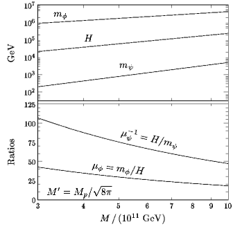
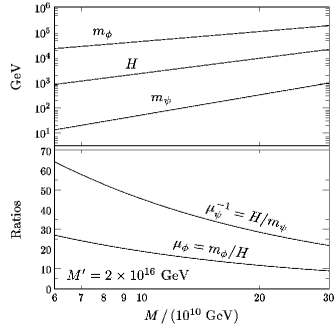
FIG. 1.: Parameter choices for supernatural inflation with $M^{\prime}$ at the Planck scale. Here $\mu_{\psi}$ is chosen to give the correct magnitude of density fluctuations for the minimum $\mu_{\psi}$ consistent with a sufficiently rapid end to inflaton.

FIG. 2.: Parameters for supernatural inflation with $M^{\prime}$ at the GUT scale. The values were chosen by the same criteria used in Fig. 1.

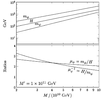
FIG. 3.: Parameters for supernatural inflation with $M^{\prime}$ at the intermediate scale.

In Figs. 1–3, we show values of the parameters when $M^{\prime}\approx M_{p}$, $M^{\prime}\approx M_{GUT}$ and $M^{\prime}\approx M_{I}$ respectively. The values shown were found by imposing the correct magnitude of density fluctuations and choosing the minimum $\mu_{\phi}\equiv m_{\phi}/H$ consistent with a sufficiently rapid end of inflation (see Sec. 6). We chose the range of $M$ to optimize parameters. Smaller $M$ would increase the values of $1/\mu_{\psi}$ and $\mu_{\phi}$. Large $M$ would improve (that is, decrease) these ratios but would make the masses uncomfortably large relative to the TeV scale. We find that smaller $M^{\prime}$ gives more natural ratios for the mass to the Hubble scale, though in all cases a ratio of less than 100 can be obtained.

These constraints assumed that the contribution of $\phi$ to density perturbations was small. In order to check the consistency of this assumption, we need to consider the evolution of $\psi$ and $\phi$ in the late stages of inflation. It will turn out that inflation must end reasonably quickly after $\psi$ reaches $\psi_{c}$ so that perturbations exit the horizon while the $\phi$ field is still confined to the origin. This gives a lower bound on $\mu_{\phi}$. In Sec. 6, we will investigate the $\phi$ mass constraint in detail.

IV Another Model

In Section 3, we investigated the possibility that there is a nonrenormalizable superpotential. However, it is frequently the case that flat directions lift each other; that is, the renormalizable potential does not permit certain field directions to be simultaneously flat. In this section, we present an alternative model with a renormalizable potential. It will turn out that this model requires a small coupling in the potential. We will motivate this assumption in Section 5, where we consider particular choices of $\psi$ and $\phi$ chosen from the supersymmetric standard model where we will show that the small coupling can actually be related to one of the known small Yukawa couplings! Once we assume this small parameter (again an unexplained but perhaps necessary parameter of the MSSM) we will find that $\mu_{\psi}$ and $\mu_{\phi}$ can both be close to unity.

So we take the potential to contain the soft supersymmetry breaking terms as before but to contain a renormalizable coupling between $\psi$ and $\phi$. Specifically

$$V=M^{4}\cos^{2}\left({\phi/\sqrt{2}f}\right)+{m_{\psi}^{2}\psi^{2}\over 2}+\lambda^{2}{\psi^{2}\phi^{2}\over 4}$$ (16)

This model has the essential features of the FDHI model of the previous section. The difference is the value of $\psi_{c}$ which in this model is

$$\psi_{c}={\sqrt{2}m_{\phi}\over\lambda}$$ (17)

The density fluctuations give the constraint

$${\lambda H^{3}e^{rN}\over m_{\psi}^{2}m_{\phi}}=1.6\cdot 10^{-4}$$ (18)

where

$$r=-{3\over 2}+\sqrt{{9\over 4}+\mu_{\psi}^{2}}\approx{\mu_{\psi}^{2}\over 3}$$ (19)

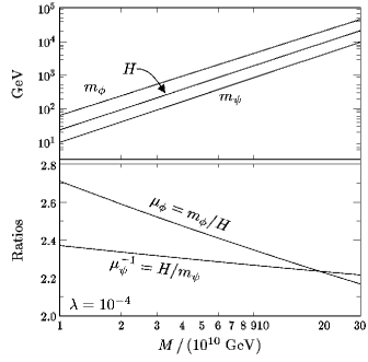
FIG. 4.: Parameter choices for supernatural inflation with renormalizable couplings, for $\lambda=10^{-4}$. Like the previous figures, this graph shows the parameters associated with the minimal allowed value of $\mu_{\phi}$.

If $\lambda$ is of order unity, to satisfy Eq. (18) requires $\mu_{\phi}>10^{3}$. However, if $\lambda\approx 10^{-4}-10^{-5}$, the model works perfectly with $\mu_{\psi}$ and $\mu_{\phi}$ both of order unity. In Fig. 4 we plot the parameters of the model for $\lambda=10^{-4}$, where again we have chosen the minimum $\mu_{\phi}$ consistent with a sufficiently quick end to inflation. We see there is virtually no fine tuning, so long as a small $\lambda$ exists(!). In the following section, we explain why such a small value for $\lambda$ is not necessarily unexpected.

V Examples of “Flat Direction” Interaction Potentials

Up to this point we have considered abstractly how to make a successful inflation model premised on properties motivated by flat direction fields. In this section, we motivate the sort of models we have considered by demonstrating examples of flat direction fields in the MSSM whose couplings are those required for a successful supernatural inflation model. However, because the $\phi$ field minimum is not at zero, which in the context of the standard model would imply large gauge symmetry breaking, the minimal standard model is not appropriate. Nevertheless, in simple extensions of the standard model, there are neutral fields which can play the role of the $\phi$ field. We will present an example of a GUT extension of the MSSM which could contain appropriate “$\psi$” and “$\phi$” fields.

We first present a few interesting cases of the form of the superpotential which arises in the context of the MSSM. Other flat direction possibilities could motivate further generalizations of the models we have studied.

Flat directions of the MSSM were considered in Ref. [16] and a complete analysis was given in Ref. [17]. They can be parameterized by gauge invariant combinations of fields. For example, the flat direction $H_{u}^{1}=H_{d}^{2}=\phi$ will be denoted as $\phi=H_{u}^{1}H_{d}^{2}$ where we have given explicit gauge indices. In each case, it is necessary to explicitly check for $F$-flatness by examining the form of the superpotential.

Example: $\psi=\bar{u_{1}}^{1}\bar{d}_{1}^{2}\bar{d}_{2}^{3}$, $\phi=Q^{1}_{2}\bar{d}_{3}^{1}L_{2}$ $W={Q\bar{u}Q\bar{d}/M^{\prime}}$. The superscripts here refer to the color indices and the subscripts to flavor indices. We haven’t specified the indices in the superpotential where in principle all allowed contractions can appear in different terms. This model would agree with the physics of our first model of inflation, except that the superpotential actually takes the form $\psi^{2}\phi X/M^{\prime}+\alpha\phi^{2}\psi X/M^{\prime}$, where $X$ is a field which is not flat and which stays at zero during the relevant stages of inflation. This can be seen by explicitly substituting $\bar{u}_{1}^{1}=\bar{d}_{1}^{2}=\bar{d}_{2}^{3}=\psi$ and $Q^{1}_{2}=\bar{d}_{3}^{1}=L_{2}=\phi$ into all possible terms of the above form in the superpotential (that is with arbitrary flavor and allowed gauge contractions). The potential will be as we have studied, except that the coefficients of the $\psi^{4}\phi^{2}$ and $\phi^{4}\psi^{2}$ terms need not be identical, since they arise from distinct terms in the superpotential, and there is a cross term which changes the exact evolution of $\phi$ but in no significant way, which arises because the separate superpotential terms can depend on the same $X$.

Example: $\psi=LH_{u}$, $\phi=H_{u}H_{d}$

In this example, SU(2) $D$ terms will lift the flat direction. This can be seen by solving for the fields in terms of the flat directions and substituting into the $D$ terms of SU(2). It can be seen that the $D$ term does not vanish, but can involve a $\psi^{2}\phi^{2}$ cross term, suppressed only by $g_{2}^{2}$, where $g_{2}$ is the SU(2) gauge coupling. As discussed in Section 4, a model of this sort with a large gauge coupling can work, but requires tuning $\mu_{\phi}$.

Example: $\psi=\bar{u}\bar{d}\bar{d}$, $\phi=LH_{u}$, $W=\lambda_{u}Q_{u}H_{u}\bar{u}$

This example realizes perfectly our scenario with a renormalizable potential generated by a small Yukawa coupling, but not a large gauge coupling. In fact, if it is indeed the up quark in the $\psi$ field, the potential works as well as could be hoped, since it depends on $\lambda_{u}^{2}\phi^{2}\psi^{2}$ which as we have shown gives $\mu_{\psi}$ and $\mu_{\phi}$ of order unity. In this model, the small size of density fluctuations arises as a natural consequence of the small up quark Yukawa coupling!

There are in fact other interactions in this model, with the field $Q_{u}$. However $Q_{u}$ is not a flat direction and is assumed to be zero (or small) throughout inflation, so that it is irrelevant to the analysis.

In fact there are many examples of the above type. Even with somewhat bigger Yukawa coupling, the correct magnitude of density fluctuations can be obtained at the expense of a larger ratio of $\mu_{\phi}$. This is probably the nicest possibility for realizing the inflationary scenario we have outlined, because the only small numbers are those already present in the form of Yukawa couplings. There are no unlikely assumptions required for the correct magnitude of density perturbations and a sufficiently rapid exit to inflation.

The problem with the MSSM as the source of inflaton candidates, as we have already stated, is that $\phi$ has a nonzero expectation value at the end of inflation. Because $\phi$ in general carries standard model gauge charge, this is not permitted. However, in GUT or other generalizations of the MSSM (or in models with completely independent fields which do not carry standard model gauge charges) one can readily realize the scenario we outlined.

Model: Consider a generalization of the standard SU(5) GUT theory to SU(6), where now the Higgs fields are in the $6$, $\bar{6}$, and $35$ ($H$, $\bar{H}$, $\Sigma$) representations of SU(6). The matter consists of three generations of $15+\bar{6}+{\bar{6}}^{\prime}$. This model has been well studied in the context of solving the doublet triplet splitting problem[18]. Examples of specific models with the requisite accidental symmetry were presented in Ref. [19].

Here we assume there is no superpotential for the $H$ and $\bar{H}$ fields, but that the potential created by the soft supersymmetry breaking terms is minimized at $\langle{H}\rangle\sim\langle{\bar{H}}\rangle\sim M_{p}$. Notice that this will break SU(6) to SU(5) which can survive to the GUT unification scale, and is therefore phenomenologically consistent. The $\Sigma$ field acquires a vacuum expectation value of order $M_{G}$. We assume that the $\Sigma$ field acquires this expectation value through renormalizable interactions, and is therefore not flat, and furthermore has reached its true minimum at the time of inflation.

Now consider $\phi=H^{0}\bar{H}^{0}$ and $\psi=15_{2}^{12}\bar{6}_{1}^{2}\bar{6^{\prime}}_{3}^{1}$ where we have labeled the matter according to its generation number (subscript) and according to the SU(6) index (superscript) (where 0 indicates the SU(5) neutral direction).

The superpotential which is required to complete the model can readily be chosen in accordance with the requirement of a small Yukawa coupling. To explicitly write the term is subtle however for two reasons. First, the leading (renormalizable terms) which give mass are the terms which make the $\bar{6}^{\prime}$ fields heavy and the term which gives the top quark a mass. However to give a renormalizable top quark coupling requires that the top be in a 20 of SU(6). All other masses arise from nonrenormalizable operators, and therefore appear more complicated. However, because of the large expectation values of the $\Sigma$, $H$, and $\bar{H}$ fields, these terms reduce to ordinary Yukawa couplings.

A toy model which would give the necessary Yukawa coupling would be $W=\lambda_{\mu}15_{2}\bar{H}\bar{6}_{2}$, where $\lambda_{\mu}\approx 10^{-3}$. This example resembles the up quark example. However, this is only a toy model because such a term actually gives the $\bar{6}^{\prime}$ a mass, and in fact defines the $\bar{6}^{\prime}$ fields. If this Yukawa coupling happens to be small, the density fluctuations would be small. Since we know little about the extra quark Yukawa coupling, we give a model involving the known quark mass parameters.

The higher dimension term $W=V_{bc}(20\Sigma)({H\over M_{P}})15_{2}$ can generate the mixing angle between the second and third generation. The effective Yukawa coupling between the flat direction fields from this term is $V_{bc}{\Sigma/M_{p}}$ which is about $10^{-4}$ (since the $\Sigma$ VEV breaks SU(5) to ${\rm SU}(3)\times{\rm SU}(2)\times{\rm U}(1)$ at the GUT scale). The density fluctuations in this model are then naturally of order $10^{-4}$.

The last model works very well, as is illustrated in Figure 4. It is extremely interesting that the inflation scenario we have devised can be explicitly realized in the context of a known model of particle physics.

VI $\psi$ and $\phi$ Evolution

In this section we will discuss the details of the evolution of $\psi$ and $\phi$. We can then derive the constraint on the $\phi$ mass.

As we have argued, inflation ends at about the time the $\phi$ squared mass changes sign at the origin so that $\phi$ will roll towards its true minimum. However, because the $\phi$ mass is not large compared to $H$ as in previous implementations of the hybrid inflation scenario [10], a careful study is required to ensure that inflation ends sufficiently rapidly that our formula for density perturbations applies. We will see that if inflation ends too slowly, perturbations will leave the Hubble radius when the $\phi$ fluctuations are large. In this scenario, if these fluctuations were on measurable scales (say greater than 1 Mpc and smaller than $10^{4}$ Mpc) either the size of density fluctuations or the deviation from a scale invariant spectrum would exceed the experimental bound. By a detailed study of the combined evolution of the $\psi$ and $\phi$ fields, we determine the necessary constraint on the $\phi$ mass for consistency of our model. However, throughout this section, it should be remembered that this constraint is only very important when $\mu_{\psi}$ is small, because it slows the transition which causes the end of inflation. When $\mu_{\psi}$ is close to unity, values of $\mu_{\phi}$ near unity are also adequate for a rapid end to inflation. For this reason, we will focus in the discussion here on the case of small $\mu_{\psi}$. We present in detail the analysis for the model of Section 3, where the constraint is more severe. A similar analysis was done for the model of Section 4 in order to obtain Figure 4.

We first consider the time evolution of $\psi$. The equation of motion for $\psi$ is

$$\ddot{\psi}+3H\dot{\psi}+m_{\psi}^{2}\psi+{\phi^{4}\over 4M^{\prime 2}}\psi=0$$ (20)

where the dot denotes derivative with respect to time $t$.

There are three relevant stages of evolution of the $\psi$ field. In the early stage of its evolution when the $\phi$ field is small (and so is $\phi^{4}/{M^{\prime}}^{2}$), the $\psi$ field obeys the slow roll equation of motion as it evolves towards the origin.

$$\psi(t)=\psi_{c}e^{-\mu_{\psi}^{2}N/3}$$ (21)

where $\psi_{c}=\sqrt{2M^{\prime}m_{\phi}}$ is the value of $\psi$ when $m_{\phi}^{2}(N=0)=0$ (at the origin) where we measure time in units of $H^{-1}$. Eventually, the $\phi$ field will grow to a sufficiently large value $\phi_{c}$, where the $\psi$ mass becomes large, and the $\psi$ field acts as a coherent state of oscillating particles with mass $m_{\psi}(t)=\phi^{2}/2M^{\prime}$. (Here we use the argument $t$ to distinguish the time-dependent physical mass of $\psi$ particles from the time-independent mass parameter in the potential.) We define $\phi_{c}$ by $\phi_{c}^{2}/2M^{\prime}=H$.

In our numerical simulations, we replace the time evolution of $\psi$ by the time evolution of its envelope at a time sufficiently late that we can neglect the term $\psi^{4}\phi^{2}/{8M^{\prime}}^{2}$ in the potential. The envelope $\psi_{e}$ obeys the approximate equation of motion

$$\dot{\psi_{e}}=-\left({3H\over 2}+{1\over 2}\Gamma(t)\right)\psi_{e}$$ (22)

where $\Gamma(t)$ is the $\psi$ decay rate, where the time dependence arises from the time dependent mass. Without further knowledge of the identity of the $\psi$ field the decay rate is an unknown parameter of the theory. We constrain the model under two reasonable scenarios for the $\psi$ decay. If $\psi$ has renormalizable couplings to other fields, its decay rate can be as large as $\Gamma_{b}\approx m_{\psi}(t)$. Of course there are unknown coefficients to this estimate but this probably represents the maximum possible rate. The true rate should lie between $\Gamma_{b}$ and $\Gamma_{l}$, where $\Gamma_{l}=m_{\psi}^{3}(t)/(M_{p}/\sqrt{8\pi})^{2}$. This latter decay rate assumes no renormalizable couplings, but Planck suppressed interactions which allow the $\psi$ field to decay. We evaluate the final stages of evolution allowing for these two possibilities for the decay rate. After the time at which $\Gamma_{\psi}\approx H$, the amplitude of the $\psi$ envelope is quickly reduced to zero, and it is only the $\phi$ field which remains. Notice that $m(t)$ could exceed $M_{p}$ before the end of inflation. However, the $\psi$ field decays well before this inconsistency in the expansion is reached.

Because of the strong dependence on the $\psi$ field of $m_{\phi}(t)^{2}=m_{\phi}^{2}(1-\psi^{4}/\psi^{4}_{c})$, the $\psi$ evolution is critical to determining the $\phi$ evolution. In the early stage of the $\phi$ evolution, it can be described by a Fokker Planck probability distribution $P(\phi,t)$. This distribution will be centered at the origin, but the spread will determine the effective amplitude of the field $\phi\equiv\sqrt{\langle\phi^{2}\rangle}$. Eventually the effective amplitude will be sufficiently large that the classical equations of motion take over. By considering the exact solution to the Fokker Planck equation, we determine the correct initial condition for the subsequent evolution of the classical field equations.

The Fokker Planck equation in a de Sitter background with time independent Hubble constant $H$ is [20]

$${dP(\phi,t)\over dt}={H^{3}\over 8\pi^{2}}\left[{d^{2}\over d\phi^{2}}\right]P(\phi,t)-{d\over d\phi}\left[{m^{2}(t)\phi\over 3H}P(\phi,t)\right]$$ (23)

where we have assumed the slow roll equation of motion to be valid. With the evolution of $\psi$ described by Eq. (21), the time-dependent mass of $\phi$ is given by

$$m_{\phi}^{2}(t)=m_{\phi}^{2}\left(1-e^{-4\mu_{\psi}^{2}Ht/3}\right)$$ (24)

The remarkable thing is that this is solvable by a Gaussian, even when the mass is time dependent.

$$P(\phi,t)={1\over\sqrt{2\pi}\sigma(t)}e^{-\phi^{2}/2\sigma(t)^{2}}$$ (25)

Here $\sigma(t)$ obeys the equation

$${d\sigma(t)\over dt}={H^{3}\over 8\pi^{2}\sigma(t)}+{m_{\phi}^{2}(t)\over 3H}\sigma(t)$$ (26)

Define $S(t)=\sigma^{2}(t)$. Then

$${dS(t)\over dt}={H^{3}\over 4\pi^{2}}+{2m_{\phi}^{2}(t)\over 3H}S(t)$$ (27)

Notice that this equation is readily interpreted as the field $\phi$ subject to the force from the classical potential (the second term) in addition to the force driving Brownian motion due to de Sitter fluctuations [21] (the first term). This equation is readily solved by finding the appropriate integrating factor and imposing the boundary condition that at $t=-\infty$, $\sigma(-\infty)=0$. The solution is

$$S(N)={H^{2}\over 4\pi^{2}}\int_{-\infty}^{N}\exp\left\{{1\over 2\xi^{2}}\left[e^{-4\mu_{\psi}^{2}N/3}-e^{-4\mu_{\psi}^{2}N^{\prime}/3}+{4\mu_{\psi}^{2}\over 3}(N-N^{\prime})\right]\right\}dN^{\prime}$$ (28)

where $\xi\equiv\mu_{\psi}/\mu_{\phi}$ and $w\equiv 1/\mu_{\psi}\mu_{\phi}$. The integrand has a peak at $N^{\prime}=0$, with a width of order $w$. When $\xi$ is small, which is generally the case in our models, the peak is nearly Gaussian and a saddle point approximation becomes applicable. So for $N$ somewhat bigger than $w$ (so that the peak is covered by the integration) and $\xi\ll 1$, $S(N)$ is well-approximated by

$$S(N)={3H^{2}w\over 4\pi^{3/2}}\exp\left\{{1\over 2\xi^{2}}\left(e^{-4\mu_{\psi}^{2}N/3}+{4\mu_{\psi}^{2}N\over 3}-1\right)\right\}\approx{3H^{2}w\over 4\pi^{3/2}}e^{4N^{2}/9w^{2}}$$ (29)

where the final approximation is valid if $w~{}\lower 2.58334pt\hbox{\vbox{\offinterlineskip\hbox{$<$}\vskip 1.0pt\hbox{$\sim$}}}~{}N\ll 1/\mu_{\psi}^{2}$.

It should be borne in mind however that the Fokker Planck equation we used incorporated the slow roll equation of motion, which is valid for $N$ small compared to $w^{2}$ Because it will turn out $w$ is not large, the Fokker Planck description will be valid only at early times. We therefore use the Fokker Planck equation to establish initial conditions, and then use the classical field equations to describe the $\phi$ evolution which we evolve numerically.

While Eq. (28) provides an analytic solution to the differential equation (27), the qualitative behavior of the solution can be seen by looking at the differential equation itself. For large negative values of $t$, $m_{\phi}^{2}(t)$ is large and negative, providing a strong restoring force. This period is characterized by quasi-equilibrium evolution, in which the restoring force holds $S(t)$ very close to its equilibrium value, $-3H^{4}/8\pi^{2}m_{\phi}^{2}(t)$, for which $dS/dt$ would vanish. The spread of this equilibrium probability distribution approaches zero in the asymptotic past, and grows monotonically with time. As $t$ approaches 0, however, this equibrium value of $S$ diverges, and the quasi-equilibrium regime ends because $S(t)$ is not able to keep up. We can estimate when the quasi-equilibrium regime ends by asking when the velocity of the equilibrium value exceeds the diffusive velocity, $H^{3}/4\pi^{2}$. For small $\xi$, this happens when $N\equiv N_{i}=-w\sqrt{9/8}$. Then $S(t)$ starts to grow diffusively, increasing linearly in time according to the first term on the right-hand side of Eq. (27). Neglecting the growth before $N=N_{i}$, which, in practice, changes the result by a number of order unity, we estimate $S(0)$ as $(H^{2}/4\pi^{2})(N-N_{i})=\sqrt{9/8}\,H^{2}w/4\pi^{2}$, which in the limit of small $\xi$ gives an answer a factor of $\sqrt{2\pi}$ smaller than the exact solution.

The diffusive regime ends when the second term on the right-hand side of Eq. (27) becomes larger than the diffusive term. This final phase can be called the classical regime, since the second term represents purely classical evolution. If only this term were included, the Fokker Planck equation would describe an ensemble of classical trajectories. This classical behavior is essential to our treatment of the problem, since it allows the description at late times to join smoothly to the full classical equations of motion which remain valid outside the slow-roll regime. The transition from the diffusive to the classical regime can be estimated by the “velocity matching criterion”, which is precisely when the two terms on the right-hand side of Eq. (27) are equal, approximating the solution until this transition by the diffusive relation $S(t)\approx H^{3}t/4\pi^{2}$. In the limit of small $\xi$, this velocity-matching condition holds at $N\equiv N_{0}=w\sqrt{9/8}$, and the value of the spread is given by $S(N_{0})\equiv\phi_{i}^{2}=3\sqrt{2}H^{2}w/16\pi^{2}$. The classical regime can be approximated by constructing a solution to the classical equations for $\phi(t)$, starting from the initial condition $\phi(N_{0})=\phi_{i}$. If the asymptotic behavior of this classical solution (in slow-roll approximation) is compared with the asymptotic behavior of $\sqrt{S(t)}$ as given by Eq. (29), it is found to be smaller by a factor of $(8\pi e)^{1/4}\approx 2.9$. In practice, we use the Fokker-Planck equation to establish the initial condition at $N_{0}$.In our numerical calculations we corrected for this discrepancy by using the initial condition $\phi(N_{0})=\bar{\phi}_{i}=(8\pi e)^{1/4}\phi_{i}$.

We have determined the time evolution of $\phi$ and $\psi$ subsequent to the velocity matching time numerically. However, as for $\psi$, the classical evolution of $\phi$ can be determined very well analytically. Again, we have to divide the analysis into three stages, according to the behavior of $\psi$.

At early times, the equation of motion for $\phi$ is approximately given by

$${d\phi\over dN}={4N\mu_{\phi}^{2}\mu_{\psi}^{2}\over 9}\phi$$ (30)

which is solved by

$$\phi(N)=\bar{\phi}_{i}e^{2(N-N_{0})^{2}/9w^{2}}$$ (31)

where we have imposed the boundary condition $\phi=\bar{\phi}_{i}$ at $N=N_{0}$. This solution has assumed slow-roll which is only approximately valid. This stage of evolution of $\phi$ lasts for $N_{1}\approx w\sqrt{9/2}\sqrt{\log(\phi_{c}/\bar{\phi}_{i})}$ $e$-folds, where $\phi_{c}=\sqrt{2M^{\prime}H}$. Numerically, we have found this answer to be off by 1-3 $e$-folds due to the correction to slow roll.

At later time, as discussed above, $\psi$ begins to oscillate. Depending on the $\psi$ decay rate, there can be several $e$-folds between this time and the time at which the $\psi$ field decays. During this range of time, it can be checked that the $\psi^{4}\phi^{2}$ term is no longer important to the equation of motion and that $\phi$ essentially keeps up with the minimum of the potential

$$V=-{m_{\phi}^{2}\phi^{2}\over 2}+{\phi^{4}\psi^{2}\over 8{M^{\prime}}^{2}}$$ (32)

and is

$$\phi(N)={\sqrt{2}m_{\phi}M^{\prime}\over\psi(N)}={\sqrt{2}m_{\phi}M^{\prime}\over\psi_{c}}e^{3N/2}=\sqrt{m_{\phi}M^{\prime}}e^{3N/2}$$ (33)

which is valid when $\Gamma\ll H$. Finally, the $\psi$ field decays. This occurs when $\Gamma\approx H$. For $\Gamma_{b}$, the number of $e$-folds during this stage is approximately $N_{2}^{b}=0$. For $\Gamma_{l}$, the value of the $\phi$ field when $\psi$ decays is approximately $\phi_{l}=(H{M^{\prime}}^{3}M_{p}^{2}/\pi)^{1/6}$. The total number of $e$-folds in this stage is approximately $2/3\log(\phi_{l}/\phi_{c})$ which is $N_{2}^{l}=(1/9)\log(M_{p}^{2}/8H^{2}\pi)$.

After $\psi$ decays, $\phi$ follows the $\psi=0$ equation of motion according to

$$\phi(t)\propto e^{rN}$$ (34)

where

$$r=\sqrt{\mu_{\phi}^{2}+{9\over 4}}-{3\over 2}$$ (35)

The number of $e$-folds in this stage is $N_{3}=(1/r)\log(\phi_{f}/\{\phi_{c},\phi_{l}\})$ depending on the decay rate, where $\phi_{f}=\pi/\sqrt{2}f$.

In fact we have checked that the solution above gives the number of $e$-folds for inflation to end correct to within 1-3 $e$-folds.

The reason we require an accurate determination of the number of $e$-foldings required for inflation to end is that it must be that the density fluctuations relevant for the observed physical scales have exited the horizon while the $\phi$ field is in the early quasi-equilibrium stage. As we will now show, the quantum fluctuations of the $\phi$ field during the diffusive regime generate a spike in the density perturbation. For the model to be viable, it is important that this spike occurs at short wavelengths, so as to avoid conflict with observations.

One interpretation of the source of density fluctuations is that the end of inflation occurs at different times at different points in space. The time delay function $\Delta\tau({\bf x})$, multiplied by $H$, is of the order of $\delta\rho/\rho$ at the time the wavelength re-enters the Hubble length. For example, if $\psi\sim e^{-m_{\psi}^{2}N/3H}$ and $\Delta\psi\sim H/2\pi$, the density fluctuation constraint would be

$$H\Delta\tau=H{\Delta\psi\over\dot{\psi}}={1\over 2\pi\sqrt{3}}{V^{3/2}\over(M_{p}/\sqrt{8\pi})^{3}V^{\prime}}={6\times 10^{-4}\over 2\pi\sqrt{3}}.$$ (36)

Since $\phi$ has a more complicated evolution, the calculation of density fluctuations at early times is subtle. The problem is to estimate the density fluctuations caused by quantum fluctuations in $\phi$ [21], whose value at times near $t=0$ is determined by the Fokker-Planck diffusion equation. Let us first consider the density fluctuations in early stages of the $\phi$ evolution. Suppose at a given time $t_{1}$ the solution $P(\phi,t)$ is modified by displacing the entire probability distribution by an amount $\Delta\phi$, so that $P_{new}(\phi,t_{1})=P_{old}(\phi-\Delta\phi,t_{1})$. We now ask how this will affect the time at which inflation ends. Because the $\psi$ and $\phi$ equations of motion are effectively decoupled, we can treat the $\psi$ field as uninfluenced, and treat the $\phi$ field as a free field evolving with time-dependent squared mass given by Eq. (24).

We guess the solution is a shifted Gaussian,

$$P(\phi,t)={1\over\sqrt{2\pi}\sigma(t)}e^{-(\phi-\bar{\phi})^{2}/2\sigma(t)^{2}}$$ (37)

We find that the Fokker-Planck equation is satisfied provided that $\sigma^{2}(t)$ obeys Eq. (27), and $\bar{\phi}(t)$ obeys the equation

$${d\bar{\phi}(t)\over dt}={m_{\phi}^{2}(t)\over 3H}\bar{\phi}$$ (38)

Imposing the initial condition $\bar{\phi}(N_{1})=\Delta\phi$, the solution to this equation is

$$\bar{\phi}(N)=\Delta\phi\exp\left[{1\over 4\xi^{2}}\left(e^{-4\mu_{\psi}^{2}N/3}-e^{-4\mu_{\psi}^{2}N_{1}/3}+{4\over 3}\mu_{\psi}^{2}\left(N-N_{1}\right)\right)\right]$$ (39)

Since the entire distribution is shifted uniformly by $\bar{\phi}(t)$, the implication is that so is each of the trajectories in the ensemble. The generic classical trajectory is the one whose value is equal to the RMS value of the distribution at large times as given by Eq. (28). Now by setting $\Delta\tau=\Delta\phi/\dot{\phi}$, we find

$$H\Delta\tau={2\sqrt{\xi}\,\Delta\phi\over H\mu_{\phi}}\left({9\pi^{3}\over e}\right)^{1/4}\left[{\exp\left[{1\over 4\xi^{2}}\left(e^{-\sqrt{2}\xi}+\sqrt{2}\xi-e^{-4\xi N_{fl}/3w}-{4\xi N_{fl}\over 3w}\right)\right]\over(1-e^{-4\xi N_{e}/3w})}\right]$$ (40)

Here $N_{fl}$ denotes the time that the initial condition is established, as the wave goes outside the Hubble length during inflation, and $N_{e}$ denotes the time at which inflation ends; both times are measured in units of $e$-foldings. This formula applies for the first type of models; the exponent has a $2\mu_{\psi}^{2}N/3$ in the second type.

The effect of a fluctuation is to determine the time and the value of $\phi$ at which diffusion ends and the classical evolution takes over ($N_{e}$). The direct change in the time at which classical evolution begins translates into a difference in time at which inflation ends. We expand the above answer for small $\xi$ to get

$$H\Delta\tau=(9\pi^{3})^{1/4}{3\over 2N_{e}}{\Delta\phi\over H}w^{3/2}e^{-2N_{fl}^{2}/9w^{2}}$$ (41)

where $N_{fl}$ is the time at which the fluctuation occurs. This falls off from the peak at $N_{fl}=0$ like a Gaussian with width $\sqrt{9w^{2}/2}$. What this tells us is that fluctuations formed sufficiently early (or late) will not delay the onset of the classical regime significantly and not give a significant contribution to density fluctuations. However, fluctuations formed during the diffusive growth regime near $N=0$ will create far too large density perturbations. These fluctuations must be such that they are not relevant to observable scales. We can observe back to about 40 $e$-folds before the end of inflation, so we require that the fluctuations formed at this time were sufficiently small, or that inflation must end by 40 $e$-folds beyond the time when the $\phi$ fluctuations satisfy the experimental bound. From Eqn. 41, one can deduce this time is approximately $N_{df}=-5w$. It might be thought that another solution is that inflation ends very slowly, so that 40 $e$-folds before the end one is in the classical regime. However, when $\phi$ is evolving according to the classical equations of motion, the scale dependence of density perturbations is much too large.

So the number of $e$-folds beyond the time when density fluctuations in $\phi$ are sufficiently small is

$$N=|N_{df}|+\sqrt{9\over 8}w+N_{1}+N_{2}+N_{3}$$ (42)

Density fluctuations on the scale of 1 Mpc are formed

$$N_{Mpc}=38+{2\over 3}\log(M/10^{11}{\rm GeV})+{1\over 3}\log(T_{RH}/10^{7}{\rm GeV})$$ (43)

$e$-folds before the end of inflation. We require that $N$ is less than $N_{Mpc}$. By following through the above calculations, one can see this gives the approximate constraint $w\approx 1$. The detailed application of the constraint gives the constraints illustrated in Figures 1-3. These plots were made assuming the larger decay rate. The total number of $e$-folds for the same parameters is generally about 5 larger with $\Gamma_{l}$ which can be accomodated with a modest change in $\mu_{\phi}$.

VII Black Holes?

Because of the large peak in the density perturbation spectrum on small length scales arising from the $\phi$ contribution, there is a danger too many small black holes being created. There are fairly strong constraints on the fractional mass density in black holes on small scales [15]. We investigate these constraints on our model in this section.

First we summarize the constraints. In the paper of Carr, Gilbert, and Lidsey, the constraints are presented in several forms; one constraint is on the parameter $\delta$ which is related to $\delta\rho/\rho$. In the mass range above $10^{30}$ gm there are bounds from CMB distortions constraining $\delta$ to be less than about $10^{-2}$. In the mass range between $10^{30}$ gm and $10^{10}$ gm the bound on $\delta$ is approximately $10^{-1.5}$. In [15] a bound due to relics is deduced constraining $\delta$ between about $10^{-2}$ and $10^{-1.5}$ in this mass range. This constraint from relics is perhaps more speculative than robust bounds from not exceeding critical density, or that decaying black holes do not produce too much entropy.

In order to apply these bounds, one needs to know the probability of black hole creation as a function of $\delta$. Based on [22], the bound is obtained from applying the formula for the probability of a region of mass $M$ forming a primordial black hole

$$\beta_{0}(M)\approx\delta(M)\exp(-{\gamma^{2}\over 2\delta^{2}})$$ (44)

where the equation of state when the perturbation enters the horizon is $p=\gamma\rho$. For the scales which are of interest to us, $\gamma=1/3$, which we will assume in the equations below.

The above bound comes from considering a spherically symmetric overdense region. The requirement is made that when the overdense region stops expanding, it’s size $S_{c}$ exceeds the Jeans radius $R_{J}$ at this time $t_{c}$, in order to collapse against the pressure. To derive exact numerical bounds on $\delta$ requires that this be the precise condition. Without solving the full problem explicitly including the pressure effects near the boundary it is difficult to state precisely the conclusion, which gives rise to some overall uncertainty in the $\delta$ bound. However, one should be able to obtain a conservative bound on $\delta$ through this approximation. However, even using this approximation, we find numerical discrepancies with the precise production rate which would be predicted. First, the relation between $t_{c}$ and $t_{0}$ (the time at which the perturbation begins to evolve separately from the homogeneous background in which it is embedded) should be $t_{c}=2t_{0}\delta^{-1}$ (the 2 being omitted in Ref. [22]) and the relation between $R_{J}$ and $t_{c}$ should be $R_{J}=2v_{s}\pi\sqrt{2/3}t_{c}$ rather than $v_{s}2t_{c}$ (in actual fact the 2 was omitted but cancels later on), where $v_{s}$ is the sound velocity. Overall this translates into the bound $\delta_{0}>v_{s}^{2}2\pi\sqrt{2/3}\left({m\over m_{0}}\right)^{-2/3}$ (where the correct relation $S_{c}=R_{0}\delta_{0}^{-1/2}$ has been substituted and the ratio $t_{0}/R_{0}$ has been replaced by the appropriate mass ratio). The implication is that the factor $\gamma^{2}/2$ in Eqn. 44 should be replaced by $4\pi^{2}\gamma^{2}/3$, which in turn decreases the strength of the bound on $\delta$ by a factor of about 5. This will of course also weaken the bound on the scalar index $n$ given in [15].

Our spectrum is not scale invariant on these small length scales which is important when calculating $\delta$ from $H\Delta\tau$. However a very conservative upper bound on our spectrum is a scale invariant spectrum starting at a small length scale (near the peak of the Gaussian) and which is constant over smaller wavelengths. This spectrum would be a scale invariant spectrum with a cutoff at large wavelength, and can readily be compared with the analysis of Ref. [15]. The normalization they use for $\delta$ can be extracted from their Eqs. (4.2)–(4.4), which express the value of $\delta$ at the COBE scale in terms of the underlying inflaton potential. Assuming that $T/S\ll 1$, their equations reduce to $\delta=0.99V^{3/2}/V^{\prime}$. By comparing with the relation $H\Delta\tau=H\delta\phi/\dot{\phi}=H^{2}/(2\pi\dot{\phi})$, one finds that $\delta$ can be related to the fluctuations in $\tau$ by $\delta=.086H\Delta\tau$. We can then apply formula 40 to find that $\delta$ (normalized as above) never exceeds 0.02, in the parameter regime presented in Figures 1-4. Because the quoted constraint on $\delta$ in [15] appears be too strong by a factor of 5, we conclude that we are consistent with reasonable estimates of the black hole constraint. Therefore, even with a conservative overestimate of $\delta$, the constraint from black holes is satisfied. However, there can be a sizable fraction of matter in black holes, which would be interesting to study in the future.

As a final comment, we remark that the bound from black holes is somewhat weaker if inflation ends more quickly, which it does for lower $w$. In fact, for $w\approx 0.5$ (corresponding to $m_{\phi}$ about four times larger than assumed) inflation ends in about 10 $e$-foldings. In this case, only the bounds from relics would apply. As this bound is more speculative, it is possible that even large perturbations on this scale would be acceptable. In reality, smaller $w$, while decreasing the length of time for inflation to end, also decreases the density perturbations. Larger $m_{\phi}$ always leads to a smaller fraction of the universe in black holes.

In summary, the black hole constraint is a serious constraint and must be accounted for. This is another constraint which would forbid large $w$, since the maximum value of $H\Delta\tau$ grows as $w^{1/2}$ (when the dependence of $N_{e}$ on $w$ is accounted for). However we have seen our model is safely within the bounds given in the literature once we have applied the $m_{\phi}$ bound given in Section 7.

However these bounds are not sufficiently precise at present and it would be interesting to do a more accurate calculation of the mass fraction in black holes both for our model and in general. The effects we have discussed should weaken existing bounds.

VIII Gravitino Constraint

In this two field model of inflation, the source of entropy and energy in the universe is the decay of the $\psi$ and $\phi$ fields. The $\psi$ field decays first, as discussed earlier. We assume the decay products are quickly thermalized, giving an effective temperature $T_{\psi}$. Sometime afterward the $\phi$ field reaches the minimum of its potential and begins to oscillate about it. We assume that these oscillations are damped by gauge or Yukawa couplings. As in Ref. [9], the decay can occur through a coupling $g^{2}/\langle\phi\rangle\int d^{4}\theta\chi^{\dagger}\chi\phi$ or through a direct Yukawa coupling $\lambda\phi\phi_{1}\phi_{2}$. This leads to a reheat temperature equal to $max(g^{2/3}m_{\phi}^{5/6}M^{1/6},m_{\phi}/\sqrt{\lambda})$, which is generally of order $10^{5}$–$10^{7}$ GeV. Since most of the energy of the universe evolves from the coherent oscillations of the $\phi$ field, this reheat temperature sets the initial conditions for the subsequent evolution. As discussed in Ref. [23], this reheat temperature is low enough to avoid the overproduction of gravitinos, even if gravitinos are as light as 100 GeV.

However, the initial temperature $T_{\psi}$ of the thermal plasma of $\psi$ decay products can be as high as $10^{11}$ GeV, so the production of gravitinos by this plasma must be examined. In this section we show that this constraint is never more restrictive than the constraints already discussed.

Gravitinos are produced by scattering processes of the thermal radiation, but interact at a rate suppressed by $m_{3/2}^{2}/M_{p}^{2}$. They are potentially dangerous since they are not thermalized and have a long lifetime. The most stringent bounds are obtained by considering the influence of these late decays on nucleosynthesis. The exact bound depends on the gravitino mass, but for $100\hbox{ GeV}~{}\lower 2.58334pt\hbox{\vbox{\offinterlineskip\hbox{$<$}\vskip 1.0pt\hbox{$\sim$}}}~{}m_{3/2}~{}\lower 2.58334pt\hbox{\vbox{\offinterlineskip\hbox{$<$}\vskip 1.0pt\hbox{$\sim$}}}~{}1\hbox{ TeV}$ it is $T_{R}<10^{7-9}{\rm GeV}$ [23].

Neglecting decay when considering gravitino production, one writes the Boltzmann equation for the gravitino number density as [23]

$${dn_{3/2}\over dt}+3Hn_{3/2}=\sigma_{\rm eff}\,n_{\rm rad}^{2}\ ,$$ (45)

where $n_{\rm rad}$ is the equilibrium number density of a single species of scalar boson ($n_{\rm rad}=\bigl{(}\zeta(3)/\pi^{2}\bigr{)}T^{3}$), and both the cross sections and the multiplicity of species are accounted for by the factor $\sigma_{\rm eff}$. In terms of $Y_{3/2}\equiv n_{3/2}/n_{\rm rad}$, we have

$${dY_{3/2}\over dt}=\sigma_{\rm eff}\,n_{\rm rad}\ .\$$ (46)

To a reasonable approximation $\sigma_{\rm eff}$ can be taken as constant, although it does vary as the coupling constants run and as species freeze out from the thermal equilibrium mix [23]. For the standard case of a radiation-dominated universe, $n_{\rm rad}\propto 1/R^{3}(t)\propto 1/t^{3/2}$ (where $R(t)$ is the scale factor), so the total gravitino production can be estimated by integrating Eq. (46) from the initial reheat time $t_{0}$ to infinity. This gives $Y_{3/2}\approx 2\sigma_{\rm eff}\,n_{{\rm rad},0}\,t_{0}=\sigma_{\rm eff}\,n_{{\rm rad},0}/H_{0}\propto T_{0}$, where the subscript $0$ refers to the time of reheating. To obtain a reasonable estimate of the present value of $Y_{3/2}$, one must divide this value by a dilution factor to account for the production of photons at times much later than $t_{0}$. According to Ref. [23], the final result is

$$Y_{3/2}(T\ll 1{\rm MeV})\approx 2.14\times 10^{-11}\left({T_{0}\over 10^{10}\hbox{ GeV}}\right)\ .$$ (47)

To derive a conservative estimate for the gravitino production of the $\psi$ decay products, we assume that the energy released by the $\psi$ decay is approximately equal to the energy stored in the oscillating $\phi$ field when inflation ends. According to the numerical simulations of our model, the fraction of energy in the $\psi$ field was generally less than this by a factor of at least $10^{4}$, except in the case $M^{\prime}=M_{p}$ and a slow decay rate, in which case $\psi$ can store a substantial fraction of the energy at the end of inflation. The universe then rapidly become matter-dominated, so $R(t)\propto t^{2/3}$. Repeating the calculation for $Y_{3/2}$ with this time evolution, one finds $Y_{3/2}={2\over 3}\,\sigma_{\rm eff}\,n_{{\rm rad},0}/H_{0}$, essentially the same formula as above.

However, in this model there is an additional dilution of the $\psi$ decay products, because the $\phi$ field behaves as a coherent state of nonrelativistic particles for a time $\Gamma_{\phi}^{-1}$, and then the $\phi$ particles decay to produce radiation. Before the $\phi$ particles decay, the energy density $\rho_{\psi}$ of the $\psi$ decay particles (assumed to be effectively massless) is suppressed relative to the energy density $\rho_{\phi}$ of the $\phi$ field by one power of the growth of the scale factor between the times $t_{0}$ and $\Gamma_{\phi}^{-1}$, which is $1/(\Gamma_{\phi}t_{0})^{2/3}$. When the $\phi$ particles decay to radiation, the number of radiation particles produced exceeds the number of $\psi$ decay particles by $(\rho_{\phi}/\rho_{\psi})^{3/4}\approx 1/(\Gamma_{\phi}t_{0})^{1/2}$. Relating $\Gamma_{\phi}$ to the $\phi$ reheat temperature $T_{R}\approx 10^{7}$ GeV and taking $t_{0}\approx 1/m_{\phi}$, the dilution factor is found to be approximately $(M_{P}m_{\phi}/T_{R}^{2})^{1/2}\approx 10^{4}$. Incorporating this extra dilution factor into Eq. (47), we find that gravitino production from $\psi$ decay products give

$$Y_{3/2}(T\ll 1\hbox{ MeV})\approx 10^{-15}\left({T_{\psi}\over 10^{10}\hbox{ GeV}}\right)\ .$$ (48)

where we have explicitly incorporated our assumption that $\psi$ and $\phi$ initially carry comparable energy.

Thus, a $\psi$ reheat temperature of $10^{11}$ GeV produces no more gravitinos then a final reheat temperature of $10^{7}$ GeV. Thus, we find that no further constraints need to be imposed.

IX Baryogenesis

In the context of late scale inflation, it is worthwhile to investigate the question of how baryons are created. There are essentially two known possibilities. Electroweak baryogenesis [24] is possible since the reheat temperature will generally be above the weak scale. Alternatively, a model in the context of supersymmetry invites investigation into the Affleck Dine scenario [25].

In the Affleck Dine baryogenesis scheme, a field $\chi$ which carries baryon number acquires a large displacement relative to its true minimum somewhere during the early evolution of the universe. If the interactions which drive the field to the true minimum are CP and $B$ violating, the field will store baryon number, and subsequently decay to baryon number carrying particles.

In our model, in principle, the fields $\phi$ or $\psi$ could be the AD fields. However this does not work. The problem is that fields which carry baryon number will generally also carry charge, so that $\phi$ is not a good possibility since charge (or color) would be spontaneously broken by the vacuum. Although $\psi$ is in principle a candidate, the ratio of baryon number stored by the $\psi$ field to entropy will be too small.

This can be deduced from a detailed study of the $\psi$ field. The first point to observe is that the potentials we have studied to now are $B$ and CP conserving. This is because we have neglected the soft “$A$” type terms and possible cross terms which can violate CP. When these are included, we find there can cause a small change in the detailed evolution of the $\phi$ field. At the time the $A$ (CP and $B$ violating terms) are large, the $\psi$ field only carried a small fraction of the energy of the universe.

However, a separate flat direction which plays the role of the AD field would work. If the AD field is independent of the inflation fields, it can then have large expectation value through the final stages of inflation. If $H$ is somewhat larger than $m_{AD}$, the analysis is similar to that in Ref. [16] where a much larger $H$ was assumed. The baryon to entropy ratio is approximately

$${n_{b}\over s}\approx{n_{b}\over n_{AD}}{T_{R}\over m_{AD}}{\rho_{AD}\over T_{R}^{4}}$$ (49)

where $n_{b}/n_{AD}$ gives the baryon to particle number ratio in the AD field, and should be order unity if the potential for the field is $B$ and CP violating. The last factor $\rho_{AD}/T_{R}^{4}$ is determined by the amplitude of the AD field at the time it evolves towards its true minimum, which is determined by higher dimension operators in the potential [16]. One can readily obtain acceptable values for the baryon density if the dimension of the operator in the superpotential which lifts the flat direction is greater than 4. The lower reheat temperature expected in these models requires a correspondingly larger factor $\rho_{AD}/T_{R}^{4}$, so a dimension 4 operator in the superpotential which lifts the AD field is insufficient.

X Discussion

There are several comments to make about the models we have considered. First there is the fact that we are considering very late inflation. We do not address the question of why the universe has lasted to this point [1]. We have only addressed the question of a late inflationary epoch responsible for solving the horizon and flatness problems and for generating the necessary density fluctuations.

One possible solution is that the initial $\psi$ value exceeds $M_{p}$. In this case, it is possible that chaotic inflation could solve the problem raised above. However, subsequent to this stage of inflation, one would expect inflation as described in this paper which would create density fluctuations of the right size.

Another point we have not addressed is what our models look like when embedded in supergravity theories. Our point of view throughout this paper is to regard the theory as an effective theory expanded in powers of $M_{p}$ (and $M^{\prime}$). We have neglected terms which are suppressed by higher powers of the Planck scale. For the same reason we have assumed a minimal Kahler potential when deriving the potential. From this point of view, any secondary minima which occur in supergravity for field values exceeding $M_{p}$ are not to be trusted.

One aspect of our models which is important is the requirement of renormalizable couplings of the fields in the $\phi$ direction in order to obtain sufficiently high reheat temperature. For this reason we expect it is more likely that the fields $\phi$ and $\psi$ correspond to flat directions of a renormalizable theory (along the lines discussed in Section 6) than to true moduli fields (of string theory) [26].

In our models, we saw that there was usually some small but not very small number. Either $M^{\prime}$ is $M_{p}$ in which case $\mu_{\psi}$ and $1/\mu_{\phi}$ are of order 100, or $M^{\prime}$ is smaller than $M_{p}$ which permits $\mu_{\psi}$ and $\mu_{\phi}$ closer to unity. Another possibility is that the small number is related to a Yukawa coupling. We discuss each of these possibilities in turn.

It is well known that there can be $H$ dependent correction to the soft supersymmetry breaking masses at early times when $H$ exceeds $m_{3/2}$ [16, 27]. This means that small $\mu_{\psi}$ is necessarily obtained by tuning. Stewart[28] has presented criteria which are sufficient for the cancellation of supergravity corrections to the inflaton mass, so that even a large ratio is technically consistent. However these conditions will only work when the scale of inflation is above the supersymmetry breaking scale. One therefore needs to invoke a new mass scale. Generally Stewart chooses the scale of gaugino condensation. It is hard to see how this scale is realized in an actual model although it could present an interesting alternative. There is a tradeoff between the complexity of the model and the “naturalness” of taking $m_{\psi}$ somewhat smaller than $H$.

In the models where $\mu_{\psi}$ is small, we found that consistency of the model required that $\mu_{\phi}$ is large, with the product $\mu_{\phi}\mu_{\psi}$ being a number of order unity. It might be thought that this large value of $\mu_{\phi}$ could be explained as due to large $H$ dependent mass corrections. However, it is not possible to introduce a large $\mu_{\phi}$ without the tuning parameter appearing in some other unnatural feature of the potential. For example, a large $H$ dependent mass could introduce a new minimum for $\phi$ which is closer to the origin so that the VEV of $\phi$ is correspondingly smaller than $M_{p}$.

We have seen however that the tuning of mass ratios is significantly reduced if we accept a higher scale than the conventional intermediate scale as setting the overall energy density. However if this scale has anything to do with visible supersymmetry breaking, the highest scale possible is probably the gaugino condensate scale. The predictions for $n$ and $R$ would be very similar, so the general test for this class of models would still be valid.

We regard the small tuning of parameters as a necessary aspect of the models with $M^{\prime}\approx M_{p}$. The necessary numbers may or may not be present. The tuning is certainly much smaller than in a typical inflation model.

On the other hand, $M^{\prime}$ might be smaller. This requires the presence of another mass scale in the theory. If this lower scale exists, one can obtain $\mu_{\psi}$ and $\mu_{\phi}$ closer to unity.

The other possibility is that there is a small Yukawa coupling. This is probably not such a bad possibility. First of all, the necessary coupling is no smaller than known Yukawa couplings and might even be related to them as in the model of Section 6 and obvious variants. Second, known Yukawas can be derived as the ratio of mass scales. In the SU(6) model we discussed this has been done in Ref. [29, 19]. It is not unreasonable to think there might be such effective Yukawa couplings in hidden sectors of the theory, as well as in the single known sector.

In most known hybrid inflation models other than the one we discussed, the $\psi$ field is very light, while the $\phi$ field is very heavy, of order $M$. This is a more serious technical problem since radiative corrections will generally give $\psi$ too large a mass [7]. Even if the model is supersymmetric, supersymmetry breaking during inflation would induce a large mass for $\psi$. Although at tree level $Str(M^{2})=0$, this is not sufficient to prevent radiative corrections at higher loop order. One can perhaps allow for such a hierarchy, but at the expense of additional complexity and mass scales. A chief advantage of our model is that both $m_{\phi}$ and $m_{\psi}$ are of order the soft supersymmetry breaking scale so this problem does not arise.

We view our model as the simplest illustration that flat directions of supersymmetric theories are consistent with the requirements of inflation when one allows for more than one field in the inflation sector. It is likely that the small parameters which might be required (of order 0.01 to 0.1) are present. Alternatively there might be more subtle mechanisms at work. Either way, one would conclude that the scale of inflation is very low. Even allowing inflation to be determined by the higher gaugino condensate scale, one would conclude that $H$ during inflation is between $10^{4}$ and $10^{7}$ GeV, and tensor perturbations are small.

It is important that there are observational consequences to this type of model. The combination of measuring the scalar index $n$ and $T/S$ should either rule out or encourage belief in the mechanism at work here. As discussed in Section 3,

$$n=1-3\left({V^{\prime}\over V}\right)^{2}+2{V^{\prime\prime}\over V}$$ (50)

Because the second term is negligible in models of the sort we are considering, where $\psi$ at the end of inflation is much less than $M_{Pl}$, it is only the last term which causes the deviation of $n$ from unity. If the dependence on $\psi$ is dominated by a mass term, as in the model of Section 3, the correction to $n$ will be positive (but small). We then expect $n$ greater than or equal to unity, and $T/S$ to be small.

XI Conclusion

We have shown that with more than one field it is possible to construct models of inflation with no small parameters. Furthermore, the mass scales which seem to most naturally appear in these models are of order $m_{3/2}$, about 1 TeV, and $M_{I}$, about $10^{11}$ GeV, leading to a natural association with supersymmetric models. These models give rise to the correctly normalized density perturbations, even though the Hubble constant is quite low, of order $10^{4}$ GeV, because the value of the inflaton field at the end of inflation is much lower than the Planck scale. The key to producing more such models is a sensitive dependence of the $\phi$ potential on the value of the $\psi$ field, so that the motion of the $\psi$ field can trigger the end of inflation while its value is small.

It seems that multifield models are probably the most natural models which can implement inflation with weak scale Hubble constant, and that furthermore, these are probably the most natural inflation models in that they involve no new small parameters. The requisite small parameters arise naturally from the ratio of mass scales. These models have the further advantages that they can be explicitly realized and one can calculate the relevant parameters for any particular implementation. They might even occur in simple extensions of the MSSM.

Perhaps the most important property of a model is its testability, and our proposed models have several characteristics that are in principle observable. The scalar index $n$ which characterizes the scale dependence of density perturbations is always greater than unity. It is very close to unity for the model of Sec. III with $M^{\prime}$ at the Planck or GUT scale, but for $M^{\prime}$ at the intermediate scale or for the model of Sec. IV, it could be as large as 1.2 for the parameters shown in our plots. In all cases tensor perturbations are negligible. An especially distinctive feature is a large spike in the density perturbation spectrum at present wavelengths of about 1 Mpc or less.

Acknowledgements

We are very grateful to Andrew Liddle, David Lyth, and Ewan Stewart for discussions and the Aspen Center for Physics where these discussions took place. We also thank Sean Carroll, Csaba Csáki, Arthur Kosowsky, Andrei Linde, and Bharat Ratra for their comments. We thank Bernard Carr, Jim Lidsey, Avi Loeb, Paul Schechter, and Paul Steinhardt for discussions and correspondence about black holes. We also thank Krishna Rajagopal for his comments on the manuscript.

REFERENCES

- [1] For a review, see A. D. Linde, Particle physics and inflationary cosmology (Harwood Academic, Switzerland, 1990).
- [2] A. Albrecht, S. Dimopoulos, W. Fischler, E.W. Kolb, S. Raby, & P.J. Steinhardt, Nucl. Phys. B229, 528 (1983)
- [3] K. Freese, J. Frieman, and A. Olinto, Phys. Rev. Lett. 65 (1990) 3233.
- [4] T. Banks, M. Berkooz, P. Steinhardt, Phys. Rev. D 52 (1995) 75.
- [5] T. Banks, M. Berkooz, G. Moore, S. Shenker, and P. Steinhardt, preprint RU-94-93, hep-th 9503114.
- [6] S. Thomas, Phys. Lett. B. 351 (1995) 424.
- [7] G. Dvali, Q. Shafi, R. Schaefer , Phys. Rev. Lett 73 (1994) 1886.
- [8] L. Randall, C. Csáki, PASCOS Proceedings (1995), hep-ph 9508208
- [9] L. Randall and S. Thomas, Nucl. Phys. B 449, 229 (1995).
- [10] A. D. Linde, Phys. Lett. B259 (1991) 38; A. R. Liddle and D. H. Lyth, Phys. Rep. 231 (1993) 1; A. D. Linde, Phys. Rev. D49 (1994) 748; E. J. Copeland, A. R. Liddle, D. H. Lyth, E. D. Stewart and D. Wands, Phys. Rev. D49 (1994) 6410; E. Stewart, Phys. Lett. B 345,414 (1995).
- [11] A. Linde, Phys. Lett. B 129, 177 (1983).
- [12] A. Guth and S.-Y. Pi, Phys. Rev. Lett. 49, 1110 (1982); A. Starobinsky, Phys. Lett. B 117, 175 (1982); S. Hawking, Phys. Lett. B 115, 295 (1982); J. Bardeen, P. Steinhardt, and M. Turner, Phys. Rev. D 28, 679 (1983).
- [13] A. R. Liddle and D. H. Lyth, astro-ph/9409077.
- [14] M. Turner, Phys. Rev. D48 (1993) 5539.
- [15] B. Carr, J. Gilbert, J. Lidsey, Phys. Rev. D 50 (1994) 4853.
- [16] M. Dine, L. Randall, and S. Thomas, Phys. Rev. Lett. 75, 398 (1995).
- [17] T. Gherghetta, C. Kolda , S. Martin, hep-ph/9510370 (1995)..
-
[18]
K. Inoue, A. Kakuto and H. Takano, Prog. Theor. Phys. 75
(1986), 664;
A. Anselm and A. Johansen, Phys. Lett. B200 (1988), 331;
A. Anselm, Sov. Phys. JETP 67 (1988), 663;
R. Barbieri, G. Dvali, A. Strumia, Nucl. Phys. B391 (1993), 487;
Z. Berezhiani and G. Dvali, Sov. Phys. Lebedev Inst. Rep. 5 (1989), 55;
R. Barbieri, G. Dvali, M. Moretti, Phys. Lett. B312 (1993), 137. - [19] Z. Berezhiani , C. Csáki, L. Randall., Nucl. Phys. B 444 (1995) 444.
- [20] A. Linde and A. Mezhulmian, gr-qc/9304015
- [21] T. Bunch and P. Davies, Proc. R. Soc. A 360, 117 (1978); A. Linde, Phys. Lett. B 116, 335 (1982); A. Starobinsky, Phys. Lett. B 117, 175 (1982); A. Linde, Phys. Lett. B 131, 330 (1983).
- [22] B. Carr, Ap. J. 201 (1975) 1.
- [23] T. Moroi, Ph.D. Thesis astro-ph/9503210, and refs. therein.
- [24] For a review see A. Cohen, D. Kaplan, and A. Nelson, Ann. Rev. Part. Nucl. Sci., 43, 27 (1993).
- [25] I. Affleck and M. Dine, Nucl. Phys. B 249, 361 (1985).
- [26] L. Dixon, in Superstrings, Unified Theories, and Cosmology 1987, Proceedings of the Summer Workshop in High energy Physics and Cosmology, eds. G. Furlan et. al., (World Scientific, Singapore, 1987).
-
[27]
M. Dine, W. Fischler, D. Nemeschansky, Phys.
Lett. B 136 (1984) 169;
O. Bertolami and G. Ross, Phys. Lett. B183 (1987)163;
E. Copeland et. al. Ref. [10]. - [28] E. Stewart, Phys. Rev. D 51 (1995) 6847.
- [29] R. Barbieri, G. Dvali, A. Strumia, Z. Berezhiani, L. Hall, Nucl. Phys. B432 (1994), 49.