BNL-62549

ISU-HET-95-9

The Decays $K\rightarrow\pi\pi\nu\overline{\nu}$ within the Standard Model

L. S. Littenberg^(a) and G. Valencia^(b)
(a) Physics Department, Brookhaven National Laboratory, Upton, NY 11973
^(b) Department of Physics, Iowa State University, Ames IA 50011

We study the reactions $K\rightarrow\pi\pi\nu\overline{\nu}$ within the minimal standard model. We use isospin symmetry to relate the matrix elements to the form factors measured in $K_{\ell 4}$. We argue that these modes are short distance dominated and can be used for precise determinations of the CKM parameters $\rho$ and $\eta$. Depending on the value of the CKM angles we find branching ratios in the following ranges: $B(K_{L}\rightarrow\pi^{+}\pi^{-}\nu\overline{\nu})=[2-5]\times 10^{-13}$; $B(K_{L}\rightarrow\pi^{0}\pi^{0}\nu\overline{\nu})=[1-3]\times 10^{-13}$; $B(K^{+}\rightarrow\pi^{+}\pi^{0}\nu\overline{\nu})=[1-2]\times 10^{-14}$. We also discuss a possible $CP$-odd observable.

Rare kaon decays have long been recognized for their potential to measure the CKM matrix parameters $\rho$ and $\eta$ as well as for their sensitivity to certain types of new interactions beyond the minimal standard model. Rare decays involving a lepton anti-lepton pair are predominantly mediated by four fermion operators that can be thought of as the product of a hadronic and leptonic currents. In this way it is possible to relate the hadronic matrix element to a measured semi-leptonic decay and avoid the uncertainties that are inherent to purely hadronic decays. This is particularly true for processes in which the leptons are neutral since they do not have long distance contributions from radiative kaon decays [1].

The short distance analysis for $|\Delta S|=1$ transitions into a $\nu\overline{\nu}$ pair has been carried out in detail before. The dominant contribution arises from penguin and box diagrams with intermediate top and charm quarks. It can be written in the form of an effective Lagrangian [2, 3]:

$${\cal L}={G_{F}\over\sqrt{2}}{\alpha\over 2\pi\sin^{2}\theta_{W}}\biggl{[}V_{cs}^{*}V_{cd}\overline{X}(x_{c},y_{\ell})+V_{ts}^{*}V_{td}X(x_{t})\biggr{]}\overline{s}\gamma_{\mu}(1-\gamma_{5})d\overline{\nu}\gamma^{\mu}(1-\gamma_{5})\nu+{\rm H.c.}$$ (1)

where the dependence on the charm-quark, top-quark and tau-lepton masses in terms of $x_{i}=M_{i}^{2}/M_{W}^{2}$ and $y_{\ell}=m_{\ell}^{2}/M_{W}^{2}$ is contained in the functions:

$$X(x_{t})={x_{t}\over 8}\biggl{[}{x_{t}+2\over x_{t}-1}+3{x_{t}-2\over(x_{t}-1)^{2}}\log x_{t}\biggr{]},$$ (2)

and $\overline{X}(x_{c},y_{\ell})$. The function $\overline{X}(x_{c},y_{\ell})$ is the analogue of Eq. 2 for a charm-quark intermediate state. In this case, however, the tau-lepton mass dependence is important as are the QCD corrections. This function cannot be written as compactly as Eq. 2 but it can be found in Ref. [3].

To compute the differential decay rate for the process $K\to\pi\pi\nu\overline{\nu}$ we need to compute the matrix element of the hadronic current $\overline{s}\gamma_{\mu}(1-\gamma_{5})d$ between the kaon and two pions states. In this note we will extract the current matrix element from the one measured in $K_{\ell 4}$ using isospin symmetry.

The standard analysis of $K_{\ell 4}$ proceeds in terms of the form factors defined by [4]:

$${\big{<}\pi^{+}(p^{+})\pi^{-}(p^{-})\big{|}\overline{s}\gamma_{\mu}\gamma_{5}u\big{|}K^{+}(k)\big{>}} = --{i\over M_{K}}\biggl{[}F(p^{+}+p^{-})_{\mu}+G(p^{+}-p^{-})_{\mu}$$ (3)

$$+R(k-p^{+}-p^{-})_{\mu}\biggr{]}$$

$${\big{<}\pi^{+}(p^{+})\pi^{-}(p^{-})\big{|}\overline{s}\gamma_{\mu}u\big{|}K^{+}(k)\big{>}} = {H\over M_{K}^{3}}\epsilon_{\mu\nu\alpha\beta}k^{\nu}(p^{+}+p^{-})^{\alpha}(p^{+}-p^{-})^{\beta}$$ (4)

The contribution of the form factor $R$ to $K_{\ell 4}$ is suppressed by the lepton mass, and $R$ does not contribute to $K\to\pi\pi\nu\overline{\nu}$. The form factors determined in $K_{e4}$ decays [5] have been found to depend on the $\pi-\pi$ invariant mass only. Theoretically, one expects these form factors to depend on all the kinematical invariants of the reaction, and this is found in a $\chi PT$ calculation [6]. The dependence of the form factors on invariants other than $M_{\pi\pi}$ may lead to interesting interference effects in the reactions $K\to\pi\pi\nu\overline{\nu}$, but we defer this discussion to a future publication. With this caveat we proceed to use the form factors measured in $K_{e4}$ in terms of the variable $q^{2}=((p^{+}+p^{-})^{2}-4m_{\pi}^{2})/4m_{\pi}^{2}$ and the $\pi-\pi$ scattering phase shifts $\delta^{I}_{J}$ [5]:

$$F = f_{s}(0)(1+\overline{\lambda}q^{2})e^{i\delta^{0}_{0}}$$

$$G = g(0)(1+\overline{\lambda}q^{2})e^{i\delta^{1}_{1}}$$

$$H = h(0)(1+\overline{\lambda}q^{2})e^{i\delta^{1}_{1}}.$$ (5)

The following constants have been measured (we use $\sin\theta_{c}=0.22$) [5]:

$$f_{s}(0) = 5.59\pm 0.14$$

$$g(0) = 4.77\pm 0.27$$

$$\overline{\lambda} = 0.08\pm 0.02$$ (6)

$$h(0) = -2.68\pm 0.68$$

The current matrix element that we need may be extracted from these measurements in the following way: when the two pions are in an $I=0$ state,

$${\big{<}\pi^{+}(p^{+})\pi^{-}(p^{-})\big{|}\overline{s}\gamma_{\mu}(1-\gamma_{5})d\big{|}K^{0}(k)\big{>}}={\big{<}\pi^{+}(p^{+})\pi^{-}(p^{-})\big{|}\overline{s}\gamma_{\mu}(1-\gamma_{5})u\big{|}K^{+}(k)\big{>}};$$ (7)

and when they are in an $I=1$ state,

$${\big{<}\pi^{+}(p^{+})\pi^{-}(p^{-})\big{|}\overline{s}\gamma_{\mu}(1-\gamma_{5})d\big{|}K^{0}(k)\big{>}}=-{\big{<}\pi^{+}(p^{+})\pi^{-}(p^{-})\big{|}\overline{s}\gamma_{\mu}(1-\gamma_{5})u\big{|}K^{+}(k)\big{>}}.$$ (8)

Using this we find that

$$A(K^{0}\to\pi^{+}\pi^{-}\nu_{\ell}\overline{\nu}_{\ell}) = -{G_{F}\over\sqrt{2}M_{K}}{\alpha\over 2\pi\sin^{2}\theta_{W}}A^{2}\lambda^{5}X(x_{t})\hat{\lambda}_{t}\overline{\nu}\gamma^{\mu}(1-\gamma_{5})\nu$$

$$\biggl{[}F(p^{+}+p^{-})_{\mu}-G(p^{+}-p^{-})_{\mu}+i{2H\over M_{K}^{2}}\epsilon_{\mu\nu\alpha\beta}k^{\nu}p^{+\alpha}p^{-\beta}\biggr{]}$$

where we have introduced the notation

$$\hat{\lambda}_{t}\approx 1-\rho-i\eta+{(1-\lambda^{2}/2)\over A^{2}\lambda^{4}}{\overline{X}(x_{c},y_{\ell})\over X(x_{t})}\equiv\rho^{0}_{\ell}-\rho-i\eta$$ (10)

and we use the Wolfenstein parameterization of the CKM matrix. From this we obtain[7]:

$$A(K_{L}\to\pi^{+}\pi^{-}\nu_{\ell}\overline{\nu}_{\ell})=-{G_{F}\over M_{K}}{\alpha\over 2\pi\sin^{2}\theta_{W}}A^{2}\lambda^{5}X(x_{t})\overline{\nu}\gamma^{\mu}(1-\gamma_{5})\nu$$ (11)

$$\times\biggl{[}F(\rho^{0}_{\ell}-\rho)(p^{+}+p^{-})_{\mu}+i\eta G(p^{+}-p^{-})_{\mu}+i{2H\over M_{K}^{2}}(\rho^{0}_{\ell}-\rho)\epsilon_{\mu\nu\alpha\beta}k^{\nu}p^{+\alpha}p^{-\beta}\biggr{]}.$$

For our numerical estimates we use $\lambda=0.22$ and $V_{cb}=0.041$ (therefore $A\approx 0.85$). Integration over phase space yields the branching ratio

$$B(K_{L}\to\pi^{+}\pi^{-}\nu\overline{\nu})=\sum_{\ell}\bigl{[}6.1(\rho^{0}_{\ell}-\rho)^{2}+0.9\eta^{2}\bigr{]}\times 10^{-14}$$ (12)

The two terms in this expression come from the contributions of the $F^{2}$ and $G^{2}$ terms in the squared matrix element. The first term corresponds to an $s$-wave, $I=0$ $\pi^{+}\pi^{-}$ pair, whereas the second term corresponds to a $p$-wave, $I=1$ $\pi^{+}\pi^{-}$ pair. The contribution of the $H^{2}$ term to $B(K_{L}\to\pi^{+}\pi^{-}\nu\overline{\nu})$ integrated over phase space has the same $\rho$ dependence as the first term in Eq. 12, but is much smaller. Unlike $K_{\ell 4}$, where it is possible to reconstruct all the momenta, in $K\to\pi\pi\nu\overline{\nu}$ only the pion momenta can be reconstructed. This reduces the number of interference terms that can actually contribute to any observable in these reactions. With the momentum dependence of the form factors that we are using, only one interference term is potentially interesting. The $F-G$ interference gives rise to a $CP$-odd $E_{\pi^{+}}-E_{\pi^{-}}$ asymmetry in the kaon rest frame. We find for the integrated asymmetry

$$A_{CP} \equiv {1\over\Gamma_{K_{L}}}\int d\Gamma(K_{L}\to\pi^{+}\pi^{-}\nu\overline{\nu}){\rm sign}[k\cdot(p^{+}-p^{-})]$$ (13)

$$\approx 3.5\times 10^{-15}\eta\sum_{\ell}(\rho^{0}_{\ell}-\rho)$$

In a similar manner we find:

$$B(K_{L}\to\pi^{0}\pi^{0}\nu\overline{\nu})=3.2\times 10^{-14}\sum_{\ell}(\rho^{0}_{\ell}-\rho)^{2},$$ (14)

reflecting the fact that the two neutral pions cannot be in an $I=1$ state; and also:

$$B(K^{+}\to\pi^{+}\pi^{0}\nu\overline{\nu})=2.3\times 10^{-15}\sum_{\ell}\bigl{[}(\rho^{0}_{\ell}-\rho)^{2}+\eta^{2}\bigr{]}.$$ (15)

This last result is an order of magnitude smaller than Eq. 12 due in part to the shorter $K^{+}$ lifetime, and in part to the approximation of Eq. 5. In particular, $p$-wave contributions to $F$ could change this result significantly.

If we use the values of Ref.[3] for the charm-quark contribution with QCD corrections to Eq. 1, and take $\Lambda_{QCD}=200$ MeV, $m_{c}=1.4$ GeV and $m_{t}=175$ GeV, we find:

$$B(K_{L}\to\pi^{+}\pi^{-}\nu\overline{\nu}) \approx \bigl{[}1.8(1.37-\rho)^{2}+0.3\eta^{2}\bigr{]}\times 10^{-13}$$

$$B(K_{L}\to\pi^{0}\pi^{0}\nu\overline{\nu}) \approx 1\times 10^{-13}\>(1.37-\rho)^{2}$$

$$B(K^{+}\to\pi^{+}\pi^{0}\nu\overline{\nu}) \approx 7\times 10^{-15}\>\bigl{[}(1.37-\rho)^{2}+\eta^{2}\bigr{]}$$

$$A_{CP} \approx 1\times 10^{-14}\>\eta(1.37-\rho)$$ (16)

Schematically, the decay $K_{L}\to\pi^{+}\pi^{-}\nu\overline{\nu}$ is induced by the operator of Eq. 1 through diagrams such as those in Figs. 1a and 1b. In these two diagrams the short-distance four-fermion operator of Eq. 1 is represented by the full crossed circle. Fig. 1a represents constant form factors and appears at lowest order in $\chi PT$, whereas contributions such as the one depicted in Fig. 1b introduce momentum dependence into the form factors and arise at higher orders in $\chi PT$.

There are also long-distance contributions to the decays $K_{L}\to\pi^{+}\pi^{-}\nu\overline{\nu}$ and we have shown some of them in Fig. 1c-f. Fig. 1c represents a charged weak current followed by a neutral weak current interaction. There are several such contributions: an eta pole can replace the pion pole; there can be higher order momentum dependence introduced as in Fig. 1d; the neutral current interaction can occur in the kaon leg as in Fig. 1e and so on. It is easy to see that these contributions are much smaller than the short distance contribution Eq. 12. For example, the diagram in Fig. 1c gives at lowest order in $\chi PT$ a contribution equivalent to having a form factor $H\approx 0.03$ in Eq. 11, much smaller than the corresponding short distance factor $h(0)(\rho^{0}_{\ell}-\rho)$. The lepton pole diagrams in Fig. 1f are also found to give a very small correction to the rate. After summing over the three leptons their contribution is: $B_{\ell}(K_{L}\to\pi^{+}\pi^{-}\nu\overline{\nu})=6.9\times 10^{-17}$.

Figure 1: Classes of diagrams that contribute to the decay $K_{L}\to\pi^{+}\pi^{-}\nu\overline{\nu}$: (a) Short distance vertex. (b) Higher order $\chi PT$ corrections to (a). (c) Long distance contribution from a charged current weak interaction followed by a neutral current weak interaction. (d) Higher order corrections to (c). (e) Long distance contribution from a neutral current weak interaction followed by a charged current weak interaction. (f) Long distance lepton-pole contribution from two charged current weak interactions.

It is amusing to note that because of the different angular momentum characteristics of the terms involving $\rho$ and $\eta$, in principle these quantities could be separately extracted from a sufficiently large sample of $K_{L}\to\pi^{+}\pi^{-}\nu\overline{\nu}$. An indication of this can be seen in Fig. 2, which shows the contrasting dependences on $\cos\theta_{\nu\bar{\nu}}^{\pi\pi}$ of the term proportional to $(\rho^{0}_{\ell}-\rho)^{2}$ and that proportional to $\eta^{2}$. Here $\theta_{\nu\bar{\nu}}^{\pi\pi}$ is the angle between the $\pi^{+}$ and vector sum of the $\nu$ and $\bar{\nu}$ momenta in the $\pi-\pi$ cm system. In practice, however, the relatively small size of the $\eta$ contribution will make it very hard to extract. Thus this process will mainly serve to determine a value for $\rho$.

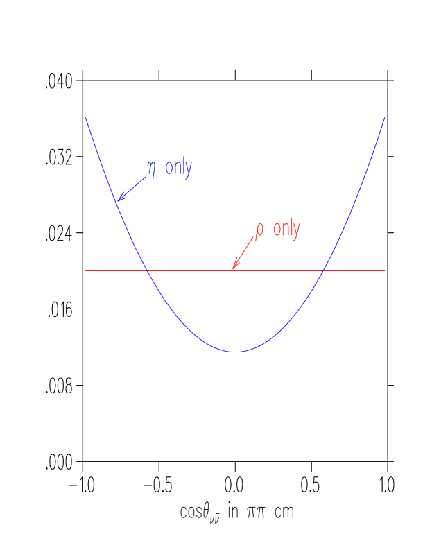
Figure 2: $d\Gamma(K_{L}\to\pi^{+}\pi^{-}\nu\overline{\nu})/d\cos\theta_{\nu\bar{\nu}}^{\pi\pi}$. $\theta_{\nu\bar{\nu}}^{\pi\pi}$ is the angle between the $\pi^{+}$ momentum and the sum of $\nu$ and $\bar{\nu}$ momenta evaluated in the $\pi^{+}\pi^{-}$ center of mass. The two terms corresponding to the $F^{2}$ (marked as $\rho$-only) and $G^{2}$ (marked as $\eta$-only) contributions are shown. The distribution given by each term has been normalized to unit area.

It is also worth pointing out that the rare decay modes we discuss in this note, $K\rightarrow\pi\pi\nu\overline{\nu}$, are complementary to the decay modes $K\rightarrow\pi\nu\overline{\nu}$ in searches for new physics. This is similar to the complementarity of $K_{L}\rightarrow\mu^{\pm}e^{\mp}$ and $K\rightarrow\pi\mu^{\pm}e^{\mp}$ in searches for lepton flavor violating interactions. The modes with one pion in the final state are only sensitive to new interactions inducing vector or scalar quark currents, whereas the modes with two pions in the final state are also sensitive to axial-vector and pseudo-scalar quark currents.

The detection of $K_{L}\to\pi^{+}\pi^{-}\nu\overline{\nu}$ will represent a major experimental challenge, particularly from the point of view of background rejection. The expected size of the branching ratio is only about an order of magnitude below the current state of the art (experiments presently running at the BNL AGS are designed to achieve a sensitivity of $10^{-12}$/event [8]). It is quite probable that a supply of $K_{L}$ sufficient to measure this process will be available within a few years. However, distinguishing this process from a number of much more copious $K_{L}$ decays may require substantial improvements in present-day photon vetoing and particle identification technology. Table 1 shows four obvious background possibilities.

Table 1: Some possible backgrounds to $K_{L}\to\pi^{+}\pi^{-}\nu\overline{\nu}$

		rejection	rejection	kinematic
Mode	BR [9]	technique	factor	rejection needed
$K_{L}\to\pi^{+}\pi^{-}\pi^{0}$	$0.1238$	photon veto	$(10^{4})^{2}$	$1.2\times 10^{4}$
$K_{L}\to\pi^{+}\pi^{-}\gamma$	$4.61\times 10^{-5}$	photon veto	$10^{4}$	$4.6\times 10^{4}$
$K_{L}\to\pi^{\mp}\mu^{\pm}\stackrel{{\scriptstyle(-)}}{{\nu}}$	$0.27$	$\mu$ ID	$10^{6}$	$2.7\times 10^{6}$
$K_{L}\to\pi^{\mp}e^{\pm}\stackrel{{\scriptstyle(-)}}{{\nu}}$	$0.387$	e ID	$10^{6}$	$3.9\times 10^{6}$

The particle ID and photon veto rejections listed are optimistic, but not out of the question for a next-generation experiment. The optimism lies less in the absolute rejections than in the notion that all can be achieved simultaneously in the same apparatus. For each background a very large factor of additional rejection is required to get to the $\sim 10^{-13}$ level. These would have to be supplied via kinematical separation. In Fig. 3 we show the differential distribution $d\Gamma(K_{L}\to\pi^{+}\pi^{-}\nu\overline{\nu})/dm_{\pi\pi}$ for typical values of $\rho$ and $\eta$. The shape of this distribution does not change significantly when we vary $\rho$ and $\eta$ over their presently allowed range. This distribution differs markedly from the corresponding ones in the background reactions listed in Table 1, but not to the extent that would allow the rejection factors listed in the rightmost column to be achieved. If one adds information on the $K_{L}$ direction, variables such as $P02$[10] can distinguish $K_{L}\to\pi^{+}\pi^{-}\nu\overline{\nu}$ from $K_{L}\to\pi^{+}\pi^{-}\pi^{0}$, but are much less effective against $K_{L}\to\pi^{+}\pi^{-}\gamma$ and $K\ell 3$. To obtain really large rejections, it will be necessary to to determine the $K_{L}$ momentum. Then, for each of the backgrounds in Table 1, one can compute a missing mass recoiling from the charged system that should be a value unique to that background[11]. Unfortunately, the $K_{L}$ momentum can only be accurately measured when it is rather low ($\leq 2$ GeV/c), whereas photon vetoing tends to be more effective at higher momenta.

Figure 3: $d\Gamma(K_{L}\to\pi^{+}\pi^{-}\nu\overline{\nu})/dm_{\pi\pi}$ for $\rho=-0.05$, $\eta=0.3$, and $A=0.85$. The shape of this distribution is quite insensitive to the values of these parameters over their presently allowed range.

Detection of $K_{L}\to\pi^{0}\pi^{0}\nu\bar{\nu}$ is likely to be even more challenging, because of the relative difficulty in reconstructing all-neutral final states, and because $B(K_{L}\to 3\pi^{0})/B(K_{L}\to\pi^{0}\pi^{0}\nu\bar{\nu})\approx 3\times B(K_{L}\to\pi^{+}\pi^{-}\pi^{0})/B(K_{L}\to\pi^{+}\pi^{-}\nu\bar{\nu})$. However there are also some advantages in the neutral case. One does not need to compromise acceptance and photon vetoing power by accommodating magnetic reconstruction and charged particle identification. What is more, certain backgrounds, such as $K_{L}\to\pi^{0}\pi^{0}\gamma$, are much smaller than their charged analogues. It would be natural to add this mode to the menu of any experiment aimed at detecting $K_{L}\to\pi^{0}\nu\bar{\nu}$, if the trigger rate allows.

In conclusion we have proposed a new, theoretically clean, way of probing the CKM parameter $\rho$. This should serve as an additional motivation for a new analysis of $K_{\ell 4}$ decays with a more detailed study of the form-factors.

After completion of this work we became aware of Ref.[12] which studies the reaction $K_{L}\rightarrow\pi^{+}\pi^{-}\nu\overline{\nu}$ using chiral perturbation theory and obtains results similar to ours. Our calculation differs from that in Ref.[12] in that we obtain the matrix elements directly from the form factors measured in $K_{\ell 4}$ using isospin symmetry. Our results are also presented in a way that we find more illuminating than that used by Ref.[12]. Ref.[12] obtains allowed ranges for the CKM angles from fits to other processes and presents final results for the rate of $K_{L}\rightarrow\pi^{+}\pi^{-}\nu\overline{\nu}$ based on those fits. Instead, we present simple numerical results in terms of the CKM angles that can be easily adapted to changing constraints on the values of the CKM parameters. We also discuss two additional modes, $K_{L}\rightarrow\pi^{0}\pi^{0}\nu\overline{\nu}$ and $K^{+}\rightarrow\pi^{+}\pi^{0}\nu\overline{\nu}$, as well as a possible $CP$-odd observable that are not studied in Ref.[12].

The work of L.L. was supported by DOE contract No. DE-AC02-76CH00016 and the work of G.V. was supported in part by the DOE OJI program under contract number DE-FG02-92ER40730. We thank John Donoghue, Mark Ito and William Marciano for useful discussions.

References

• [1] See for example J.Β Hagelin and L.Β Littenberg, Prog. Part. Nucl. Phys. 23 1 (1989); L.Littenberg and G. Valencia, Ann. Rev. Nucl. Part. Sci. 43 729 (1993); R.Β Battiston, et. al., Phys. Rep. 214 293 (1992); J.Β Ritchie and S.Β Wojcicki, Rev. of Mod. Phys. 65 1149 (1993); and references therein.
• [2] T.Β Inami and C.Β S.Β Lim, Prog. Theo. Phys. 65 297 (1981); E.65 1772 (1981).
• [3] G.Β Buchalla, A.Β Buras and M.Β Harlander, Nucl. Phys. B349 1 (1991); G.Β Buchalla and A.Β Buras, Nucl. Phys.B412 106 (1994).
• [4] A.Β Pais and S.Β B.Β Treiman, Phys. Rev.168 1858 (1968).
• [5] L.Β Rosselet et. al., Phys. Rev.D15 574 (1977).
• [6] J.Β Bijnens, Nucl. Phys.B337 635 (1990); C.Β Riggenbach et. al., Phys. Rev.D43 127 (1991).
• [7] We assume CPT invariance and we drop a very small contribution from $CP$ violation in the $K^{0}-\overline{K}^{0}$ mass matrix.
• [8] M.E.Β Zeller, et al., AGS Proposal 865 (1990); A.Β Heinson, et al., AGS Proposal 871 (1990).
• [9] L.Β Montanet, et al., Phys.Β Rev. D50 1173 (1994).
• [10] This commonly used variable is defined as $P02\equiv[(m_{K}^{2}-m_{\pi^{0}}^{2}-m_{\pi\pi}^{2})^{2}-4m_{\pi^{0}}^{2}m_{\pi\pi}^{2}-4m_{K}^{2}(P_{\pi\pi}^{T})^{2}]/[(P_{\pi\pi}^{T})^{2}+m_{\pi\pi}^{2}]$, where $m_{\pi\pi}$ is the effective mass of the charged $\pi$ system and $P_{\pi\pi}^{T}$ is the component of the vector sum of the pion momenta transverse to the $K_{L}$ direction.
• [11] To identify $K\ell 3$, one must assign the lepton mass to each charged track in turn; one combination will give missing mass $\approx 0$.
• [12] C.Q.Β Geng, I.J.Β Hsu and Y.C.Β Lin, Phys. Rev. D50 5744 (1994).