TTP95-47
December 1995
hep-ph/9512409

POLARIZED TOP QUARKS
M. JEŻABEK

Institute of Nuclear Physics, Kawiory 26a, PL-30055 Cracow, Poland
and

R. HARLANDER, J. H. KÜHN and M. PETER

Institut für Theoretische Teilchenphysik, Universität Karlsruhe
D-76128 Karlsruhe, Germany

ABSTRACT

Recent calculations are presented of top quark polarization in $t\bar{t}$ pair production close to threshold. S–P-wave interference gives contributions to all components of the top quark polarization vector. Rescattering of the decay products is considered. Moments of the fourmomentum of the charged lepton in semileptonic top decays are calculated and shown to be very sensitive to the top quark polarization.

1 Introduction

Threshold production of top quarks at a future electron–positron collider will allow to study their properties with extremely high precision. The dynamics of the top quark is strongly influenced by its large width $\Gamma_{t}\approx 1.5$ GeV. Individual quarkonium resonances can no longer be resolved, hadronization effects are irrelevant and an effective cutoff of the large distance (small momentum) part of the hadronic interaction is introduced^?,?,?. This in turn allows to measure the short distance part of the potential, leading to a precise determination of the strong coupling constant^?. The analysis of the total cross section combined with its momentum distribution will determine its mass with an accuracy of at least 300 MeV and its width to about 10%. For a Higgs boson mass of order 100 GeV even the $t\bar{t}H$ Yukawa coupling could be indirectly deduced from its contribution to the vertex correction^?. Additional constraints on these parameters can be derived from the forward–backward asymmetry of top quarks and from measurements of the top quark spin. Close to threshold, for $E=\sqrt{s}-2m_{t}\ll m_{t}$, the total cross section and similarly the momentum distribution of the quarks are essentially governed by the $S$-wave amplitude, with $P$-waves suppressed $\sim\beta^{2}\sim\sqrt{E^{2}+\Gamma_{t}^{2}}/m_{t}\approx 10^{-2}$. The forward–backward asymmetry and, likewise, the transverse component of the top quark spin originate from the interference between $S$- and $P$-wave amplitudes and are, therefore, of order $\beta\approx 10^{-1}$ even close to threshold. Note that the expectation value of the momentum is always different from zero as a consequence of the large top width and the uncertainty principle, even for $E=0$.

It has been demonstrated^?,? that the Green function technique is particularly suited to calculate the total cross section in the threshold region. The method has been extended^?,? to predict the top quark momentum distribution. A further generalization then leads to the inclusion of $P$-waves and, as a consequence, allows to predict the forward–backward asymmetry^?. It has been shown^? that the same function $\varphi_{{}_{R}}({\bf p},E)$ which results from the $S$–$P$-wave interference governs the dynamical behaviour of the forward–backward asymmetry as well as the angular dependence of the transverse part of the top quark polarization. The close relation between this result and the tree level prediction, expanded up to linear terms in $\beta$, has been emphasised. The relative importances of $Z$ versus $\gamma$ and of axial versus vector couplings depend on the electron (and/or positron) beam polarization. All predictions can, therefore, be further tested by exploiting their dependence on beam polarization. In fact the reaction $e^{+}e^{-}\to t\bar{t}$ with longitudinally polarized beams is the most efficient and flexible source of polarized top quarks. At the same time the longitudinal polarization of the electron beam is an obvious option for a future linear collider. Recently^? these results have been expanded in two directions:

• Normal polarization. Calculation of the polarization normal to the production plane is a straightforward extension of the previous work^? and is based on the same nonrelativistic Green function as before, involving, however, the imaginary part of the interference term $\varphi_{{}_{I}}({\bf p},E)$. A component of the top quark polarization normal to the production plane may also be induced by time reversal odd components of the $\gamma t\bar{t}$- or ${\rm Z}t\bar{t}$-coupling with an electric dipole moment as most prominent example. Such an effect would be a clear signal for physics beyond the standard model. The relative sign of particle versus antiparticle polarizations is opposite for the QCD-induced and the $T$-odd terms respectively, which allows to discriminate the two effects. Nevertheless it is clear that a complete understanding of the QCD-induced component is mandatory for a convincing analysis of the $T$-odd contribution.

• Rescattering. Both $t$ quark and $\bar{t}$ antiquark are unstable and decay into $W^{+}b$ and $W^{-}\bar{b}$, respectively. Neither $b$ nor $\bar{b}$ can be considered as freely propagating particles. Rescattering in the $t\bar{b}$ and $b\bar{t}$ systems affects not only the momenta of the decay products but also the polarization of the top quark. Moreover, in the latter case, when the top quark decays first and its colored decay product $b$ is rescattered in a Coulomb-like chromostatic potential of the spectator $\bar{t}$, the top polarization is not a well defined quantity. Instead one can consider other quantities, like the total angular momentum of the $Wb$ subsystem, which are equal to the spin of top quark in the situation when rescattering is absent. These rescattering corrections are suppressed by $\alpha_{s}$. The resulting modifications of the momentum distribution are therefore relatively minor and as far as the total cross section is concerned can even be shown to vanish^?. In contrast the forward–backward asymmetry as well as the transverse and normal parts of the top quark spin are suppressed by a factor $\sim\beta$. Thus, they are relatively more sensitive towards rescattering corrections. Rescattering in the $b\bar{b}$ system is less important and will be neglected.

It is well known^? that the direction of the charged lepton in semileptonic decays is the best polarization analyzer for the top quark. The reason is^? that in the top quark rest frame the double differential energy–angular distribution of the charged lepton is a product of the energy and the angular dependent factors. The angular dependence is of the form $(1+P\cos\theta)$, where $P$ denotes the top quark polarization and $\theta$ is the angle between the polarization three-vector and the direction of the charged lepton. Gluon radiation and virtual corrections in the top quark decay practically do not affect these welcome properties^?. It is therefore quite natural to perform polarization studies by measuring the inclusive distributions of say $\mu^{+}$ in the process $e^{+}e^{-}\to t(\mu^{+}\nu_{\mu}b)\bar{t}(jets)$. This can be also convenient from the experimental point of view because there is no missing energy-momentum for the $\bar{t}$ subsystem. From the theoretical point of view the direction of the charged lepton can be considered as another quantity which is equivalent to the top quark polarization when rescattering is absent. Of course, it is well defined also in the case of $b\bar{t}$ rescattering. However, the semi-analytic calculation of the latter contribution is a very difficult task because production and decay mechanisms are coupled. A way out^? is to calculate moments of the charged lepton four-momentum distributions. The results of this analysis are published elsewhere^?.

2 Green functions, angular distributions and quark polarization

2.1 The nonrelativistic limit

Top quark production in the threshold region is conveniently described by the Green function method which allows to introduce in a natural way the effects of the large top decay rate $\Gamma_{t}$ and avoids the summation of many overlapping resonances. The total cross section can be obtained from the imaginary part of the Green function $G({\bf x}=0,{\bf x}^{\prime}=0,E)$ via the optical theorem. To predict the differential momentum distribution, however, the complete ${\bf x}$-dependence of $G({\bf x},{\bf x}^{\prime}=0,E)$ (or, more precisely, its Fourier transformed) is required. In a calculation with non-interacting quarks close to threshold the forward–backward asymmetry, the leading angular dependent term $\sim\cos\vartheta$ and the transverse part of the top quark polarization are all proportional to the quark velocity $\beta$ and originate from the interference of a $S$-wave with a $P$-wave amplitude. These distributions are described by $\nabla^{\prime}\cdot G({\bf x},{\bf x}^{\prime},E)|_{{\bf x}^{\prime}=0}$ or, equivalently, by the component of the Green function with angular momentum one. The connection between the relativistic treatment and the nonrelativistic Lippmann–Schwinger equation has been discussed in the literature^?,?. The subsequent discussion follows these lines. It includes, however, also the spin degrees of freedom and is, furthermore, formulated sufficiently general such that it is immediately applicable to other reactions of interest. The main ingredient in the derivation of the nonrelativistic limit is the ladder approximation for the vertex function $\Gamma_{\cal C}$. This vertex function is the solution of the following integral equation depicted in Fig.1:

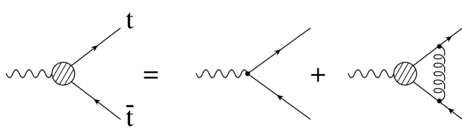
Figure 1: Lippmann–Schwinger equation in diagrammatical form.

$$\Gamma_{\cal C}={\cal C}+\int{d^{4}k\over(2\pi)^{4}}\left(-{4\over 3}4\pi\alpha_{s}\right)D_{\mu\nu}(p-k)\gamma^{\mu}S_{\rm F}(k+{q\over 2})\Gamma_{\cal C}(k,q)S_{\rm F}(k-{q\over 2})\gamma^{\nu},$$ (1)

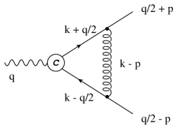
Figure 2: Definition of the four-momenta.

with ${\cal C}=\gamma_{\mu}$ or $\gamma_{\mu}\gamma_{5}$ in the cases of interest for $e^{+}e^{-}$-annihilation. The conventions for the flow of momenta are illustrated in Fig.2. The four-momenta are related to the nonrelativistic variables by

$$q = (2m_{t}+E,{\bf 0})$$

$$p = (0,{\bf p})$$ (2)

$$k = (k_{0},{\bf k}).$$

In perturbation theory the ladder approximation is motivated by the observation that for each additional rung the energy denominator after loop integration compensates the coupling constant attached to the gluon propagator. This is demonstrated most easily in Coulomb gauge. Contributions from transverse gluons as well as those from other diagrams are suppressed by higher powers of $\beta\sim\alpha_{s}$. The gluon propagator is thus replaced by the instantaneous nonrelativistic potential

$${4\over 3}\,4\pi\alpha_{s}D_{\mu\nu}(p)\rightarrow i\,V({\bf p})\,\delta_{\mu 0}\delta_{\nu 0}.$$ (3)

The dominant contribution to the integral originates from the region where $|{\bf k}|\ll m_{t}$. Including terms linear in ${\bf k}$, quark and antiquark propagators are approximated by
$\displaystyle\hskip 43.05542ptS_{\rm F}(k+{q\over 2})$ $\displaystyle=$ $\displaystyle i{\Lambda_{+}-{{\bf k}\cdot\mbox{\boldmath\scriptsize$\gamma$}\over 2m_{t}}\over{E\over 2}+k_{0}-{{\bf k}^{2}\over 2m_{t}}+i{\Gamma_{t}\over 2}}$ $\displaystyle S_{\rm F}(k-{q\over 2})$ $\displaystyle=$ $\displaystyle i{\Lambda_{-}-{{\bf k}\cdot\mbox{\boldmath\scriptsize$\gamma$}\over 2m_{t}}\over{E\over 2}-k_{0}-{{\bf k}^{2}\over 2m_{t}}+i{\Gamma_{t}\over 2}}\,,$ $\displaystyle\Lambda_{\pm}$ $\displaystyle=$ $\displaystyle{1\pm\gamma^{0}\over 2}\,.$ The “elementary” vertex ${\cal C}$ is independent of $k_{0}$. (Within the present approximations this is even true if ${\cal C}$ does depend on ${\bf k}$ as is the case in the analogous treatment of $\gamma\gamma\to t\bar{t}$ discussed below.) Up to and including order $\beta$ terms a selfconsistent solution of the integral equation (1) can be obtained if $\Gamma_{\cal C}$ is taken independent of $k_{0}$ and the nonrelativistic spins of $t$ and $\bar{t}$. The $k_{0}$ integration is then easily performed and the integral equation simplified to

$$\Gamma_{\cal C}={\cal C}+\int{d^{3}k\over(2\pi)^{3}}V({\bf p}-{\bf k})\gamma^{0}(\Lambda_{+}-{{\bf k}\cdot\gamma\gamma\gamma\over 2m_{t}}){\Gamma_{\cal C}({\bf k},E)\over E-{{\bf k}^{2}\over m_{t}}+i\Gamma_{t}}(\Lambda_{-}-{{\bf k}\cdot\gamma\gamma\gamma\over 2m_{t}})\gamma^{0}.$$ (5)

In the calculation of the cross section for the production of $t$ plus $\bar{t}$ with momenta $q/2\pm p$ and spins $s_{\pm}$ respectively traces ${\cal H}$ of the following structure will arise:

$${\cal H} = {\rm Tr}\{{\cal P}_{+}({q\over 2}+p,s_{+})\Gamma_{\cal C}{\cal P}_{-}({q\over 2}-p,s_{-})\bar{\Gamma}_{{\cal C}^{\prime}}\},$$ (6)

$${\cal P}_{\pm}(p,s) = {\mbox{$p/$}\pm m_{t}\over 2m_{t}}\,{1+\gamma_{5}\mbox{$s/$}\over 2},$$ (7)

where we allowed for mixed terms with ${\cal C}$ different from ${\cal C}^{\prime}$. Expanding again up to terms linear in ${\bf k}$, this trace can be transformed into

$${\cal H} = {\rm Tr}\{{\cal S}_{+}\widetilde{\Gamma}_{\cal C}{\cal S}_{-}\bar{\widetilde{\Gamma}}_{{\cal C}^{\prime}}\},$$ (8)

$${\cal S}_{\pm} = {1\pm{\bf s}_{\pm}\cdot\mbox{\boldmath$\Sigma$}\over 2},$$ (9)

$$\Sigma = \gamma\gamma\gamma\gamma_{5}\gamma^{0}=\left(\begin{array}[]{cc}\mbox{\boldmath$\sigma$}&0\\ 0&\mbox{\boldmath$\sigma$}\end{array}\right),$$ (12)

with the nonrelativistic reduction defined through

$$\widetilde{\Gamma}_{\cal C}({\bf p},E)=\Lambda_{+}\,(1-{{\bf p}\cdot\gamma\gamma\gamma\over 2m_{t}})\,\Gamma_{\cal C}({\bf p},E)\,(1-{{\bf p}\cdot\gamma\gamma\gamma\over 2m_{t}})\,\Lambda_{-}.$$ (13)

It is thus sufficient to calculate the “reduced” vertex function $\widetilde{\Gamma}_{\cal C}$. Dropping again terms of order ${\bf k}^{2}$, the corresponding integral equation is cast into a particularly simple form

$$\widetilde{\Gamma}_{\cal C}({\bf p},E)=\widetilde{{\cal C}}({\bf p})+\int{d^{3}k\over(2\pi)^{3}}V({\bf p}-{\bf k}){\widetilde{\Gamma}_{\cal C}({\bf k},E)\over E-{{\bf k}^{2}\over m_{t}}+i\Gamma_{t}}.$$ (14)

Consistent with the nonrelativistic approximation only the constant and the linear term in the Taylor expansion of the elementary vertex will be considered

$$\widetilde{{\cal C}}({\bf p})=\widetilde{{\cal C}}(0)+{\bf D}\cdot{\bf p}$$ (15)

The matrices $\widetilde{\cal C}(0)$ and ${\bf D}$ may in general depend on external momenta, polarization vectors or Lorentz indices. A selfconsistent solution for the vertex $\widetilde{\Gamma}_{\cal C}$ is then given by

$$\widetilde{\Gamma}_{\cal C}({\bf p},E)=\widetilde{\cal C}(0){\cal K}_{\rm S}({\rm p},E)+{\bf D}\cdot{\bf p}\,{\cal K}_{\rm P}({\rm p},E)$$ (16)

The scalar vertex functions ${\cal K}_{\rm S,P}$ depend on

$${\rm p}=|{\bf p}|$$

and $E$ only. They are solutions of the nonrelativistic integral equations

$${\cal K}_{\rm S}({\rm p},E) = 1+\int{d^{3}k\over(2\pi)^{3}}V({\bf p}-{\bf k}){{\cal K}_{\rm S}({\rm k},E)\over E-{{\bf k}^{2}\over m_{t}}+i\Gamma_{t}}$$ (17)

$${\cal K}_{\rm P}({\rm p},E) = 1+\int{d^{3}k\over(2\pi)^{3}}{{\bf p}\cdot{\bf k}\over{\bf p}^{2}}V({\bf p}-{\bf k}){{\cal K}_{\rm P}({\rm k},E)\over E-{{\bf k}^{2}\over m_{t}}+i\Gamma_{t}}$$ (18)

and are closely related to the Green function ${\cal G}({\bf p},{\bf x},E)$ which, in turn, is a solution of the Lippmann–Schwinger equation

$$\bigg{[}E-{{\bf p}^{2}\over m_{t}}+i\Gamma_{t}\bigg{]}{\cal G}({\bf p},{\bf x},E)=e^{i{\bf p}\cdot{\bf x}}+\int{d^{3}k\over(2\pi)^{3}}V({\bf p}-{\bf k}){\cal G}({\bf k},{\bf x},E).$$ (19)

Let us denote the first two terms of the Taylor series with respect to ${\bf x}$ by $G$ and $F$ respectively:

$${\cal G}({\bf p},{\bf x},E)=G({\rm p},E)+{\bf x}\cdot{\bf p}\,F({\rm p},E)+\ldots$$

They are solutions of the integral equations

$$G({\rm p},E) = G_{0}({\rm p},E)+G_{0}({\rm p},E)\int{d^{3}k\over(2\pi)^{3}}V({\bf p}-{\bf k})G({\rm k},E)$$ (20)

$$F({\rm p},E) = G_{0}({\rm p},E)+G_{0}({\rm p},E)\int{d^{3}k\over(2\pi)^{3}}{{\bf p}\cdot{\bf k}\over{\bf p}^{2}}V({\bf p}-{\bf k})F({\rm k},E),$$ (21)

with

$$G_{0}({\rm p},E)={1\over E-{{\bf p}^{2}\over m_{t}}+i\Gamma_{t}},$$ (22)

and the relation between Green function and vertex function

$$G({\rm p},E)=G_{0}({\rm p},E){\cal K}_{\rm S}({\rm p},E),\qquad F({\rm p},E)=G_{0}({\rm p},E){\cal K}_{\rm P}({\rm p},E)$$ (23)

is evident. In the case of $e^{+}e^{-}$-annihilation top production proceeds through the space components of the vector and axial vector current. The relevant elementary vertex $\widetilde{\cal C}({\bf p})$ is given by

$$\widetilde{\gamma_{j}}({\bf p}) = \Lambda_{+}\gamma_{j}\Lambda_{-}$$ (24)

$$\widetilde{\gamma_{j}\gamma_{5}}({\bf p}) = \Lambda_{+}({i\over m_{t}})(\mbox{\boldmath$\gamma$}\times{\bf p})_{j}\Lambda_{-}$$ (25)

for vector and axial current respectively. Production of $t\bar{t}$ in $\gamma\gamma$-fusion would lead to an elementary vertex of the form

$$\widetilde{{\cal C}}(0) \propto i(\mbox{\boldmath$\epsilon$}_{1}\times\mbox{\boldmath$\epsilon$}_{2})\,{\bf n}_{e^{-}}\Lambda_{+}\gamma_{5}\Lambda_{-}$$ (26)

$${\bf D} \propto {1\over m_{t}}\Lambda_{+}\left[(\mbox{\boldmath$\epsilon$}_{1}\cdot\mbox{\boldmath$\epsilon$}_{2})({\bf n}_{e^{-}}\cdot\gamma\gamma\gamma){\bf n}_{e^{-}}+(\mbox{\boldmath$\epsilon$}_{2}\cdot\gamma\gamma\gamma)\,\mbox{\boldmath$\epsilon$}_{1}+(\mbox{\boldmath$\epsilon$}_{1}\cdot\gamma\gamma\gamma)\,\mbox{\boldmath$\epsilon$}_{2}\right]\Lambda_{-},$$ (27)

with $\mbox{\boldmath$\epsilon$}_{1}$, $\mbox{\boldmath$\epsilon$}_{2}$ the polarization vectors of the photons, and the present formalism applies equally well. This case has been studied by Fadin et al.^?.

2.2 Top production in electron positron annihilation

With these ingredients it is straightforward to calculate the differential momentum distribution and the polarization of top quarks produced in electron positron annihilation. Let us introduce the following conventions for the fermion couplings

$$v_{f}=2I^{3}_{f}-4q_{f}\sin^{2}\theta_{W},\qquad a_{f}=2I^{3}_{f}.$$ (28)

$P_{\pm}$ denotes the longitudinal electron/positron polarization and

$$\chi={P_{+}-P_{-}\over 1-P_{+}P_{-}}$$ (29)

can be interpreted as effective longitudinal polarization of the virtual intermediate photon or $Z$ boson. The following abbreviations will be useful below:

$$a_{1} = q_{e}^{2}q_{t}^{2}+(v_{e}^{2}+a_{e}^{2})v_{t}^{2}d^{2}+2q_{e}q_{t}v_{e}v_{t}d$$

$$a_{2} = 2v_{e}a_{e}v_{t}^{2}d^{2}+2q_{e}q_{t}a_{e}v_{t}d$$

$$a_{3} = 4v_{e}a_{e}v_{t}a_{t}d^{2}+2q_{e}q_{t}a_{e}a_{t}d$$

$$a_{4} = 2(v_{e}^{2}+a_{e}^{2})v_{t}a_{t}d^{2}+2q_{e}q_{t}v_{e}a_{t}d$$

$$d = {1\over 16\sin^{2}\theta_{W}\cos^{2}\theta_{W}}\,{s\over s-M_{Z}^{2}}.$$

The differential cross section, summed over polarizations of quarks and expanded up to terms linear in ${\bf p}$, is thus given by

$${d\sigma\over d{\bf p}} = {3\alpha^{2}\Gamma_{t}\over 4\pi m_{t}^{4}}(1-P_{+}P_{-})\left[{(a_{1}+\chi a_{2})\left(1-{16\alpha_{s}\over 3\pi}\right)\left|G({\rm p},E)\right|^{2}+}\right.$$ (30)

$$\left.{+(a_{3}+\chi a_{4})\left(1-{12\alpha_{s}\over 3\pi}\right){{\rm p}\over m_{t}}{\rm Re}\left(\,G({\rm p},E)F^{*}({\rm p},E)\,\right)\,\cos\vartheta}\right].$$

The vertex corrections from hard gluon exchange for $S$-wave^? and $P$-wave^? amplitudes are included in this formula. It leads to the following forward–backward asymmetry

$${\cal A}_{\rm FB}({\rm p},E)=C_{\rm FB}(\chi)\,\varphi_{{}_{R}}({\rm p},E),$$ (31)

with

$$C_{\rm FB}(\chi)={1\over 2}\,{a_{3}+\chi a_{4}\over a_{1}+\chi a_{2}},$$ (32)

$\varphi_{{}_{R}}({\rm p},E)={\rm Re}\,\varphi$, and

$$\varphi({\rm p},E)={(1-{4\alpha_{s}/3\pi})\over(1-{8\alpha_{s}/3\pi})}\,{{\rm p}\over m_{t}}\,{F^{*}\!({\rm p},E)\over G^{*}\!({\rm p},E)}.$$ (33)

This result is still differential in the top quark momentum. Replacing $\varphi({\rm p},E)$ by

$$\Phi(E)={(1-{4\alpha_{s}/3\pi})\over(1-{8\alpha_{s}/3\pi})}\,{\int_{0}^{{\rm p}_{m}}d{\rm p}\,{{\rm p}^{3}\over m_{t}}\,F^{*}({\rm p},E)G({\rm p},E)\over\int_{0}^{{\rm p}_{m}}d{\rm p}\,{\rm p}^{2}\left|G({\rm p},E)\right|^{2}}.$$ (34)

one obtains the integrated forward–backward asymmetry. The cutoff ${\rm p}_{m}$ must be introduced to eliminate the logarithmic divergence of the integral. For free particles (or sufficiently far above threshold) one finds for example

$$\Phi(E)=\sqrt{\frac{E}{m_{t}}}+\frac{2\Gamma_{t}}{\sqrt{m_{t}E}\pi}\ln{\rm p}_{m}/m_{t}$$ (35)

This logarithmic divergence is a consequence of the fact that the nonrelativistic approximation is used outside its range of validity. On may either choose a cutoff of order $m_{t}$ or replace the nonrelativistic phase space element ${\rm p}\,d{\rm p}/m_{t}$ by ${\rm p}\,d{\rm p}/\sqrt{m_{t}^{2}+{\rm p}^{2}}$. In practical applications a cutoff will be introduced by the experimental procedure used to define $t\bar{t}$-events.

2.3 Polarization

To describe top quark production in the threshold region it is convenient to align the reference system with the beam direction (Fig.3) and to define

$${\bf s}_{\|} = {\bf n}_{e^{-}}$$

$${\bf s}_{\rm N} = {{\bf n}_{e^{-}}\times{\bf n}_{t}\over|{\bf n}_{e^{-}}\times{\bf n}_{t}|}$$ (36)

$${\bf s}_{\bot} = {\bf s}_{\rm N}\times{\bf s}_{\|}.$$

Figure 3: Definition of the spin directions. The normal component ${\bf s}_{\rm N}$ points out of the plane.

In the limit of small $\beta$ the quark spin is essentially aligned with the beam direction apart from small corrections proportional to $\beta$, which depend on the production angle. A system of reference with ${\bf s}_{\|}$ defined with respect to the top quark momentum^? is convenient in the high energy limit but evidently becomes less convenient close to threshold.

Including the QCD potential one obtains for the three components of the polarization

$${\cal P}_{\|}({\bf p},E,\chi) = C_{\|}^{0}(\chi)+C_{\|}^{1}(\chi)\,\varphi_{{}_{R}}({\rm p},E)\,\cos\vartheta\,$$ (37)

$${\cal P}_{\bot}({\bf p},E,\chi) = C_{\bot}(\chi)\,\varphi_{{}_{R}}({\rm p},E)\,\sin\vartheta\,$$ (38)

$${\cal P}_{\rm N}({\bf p},E,\chi) = C_{\rm N}(\chi)\varphi_{{}_{I}}({\rm p},E)\sin\vartheta\,,$$ (39)

$$\hskip 21.52771ptC_{\|}^{0}(\chi)=-{a_{2}+\chi a_{1}\over a_{1}+\chi a_{2}},\hskip 29.7082ptC_{\|}^{1}(\chi)=\left(1-\chi^{2}\right){a_{2}a_{3}-a_{1}a_{4}\over\left(a_{1}+\chi a_{2}\right)^{2}},$$

$$\hskip 21.52771ptC_{\bot}(\chi)=-{1\over 2}\,{a_{4}+\chi a_{3}\over a_{1}+\chi a_{2}},\qquad C_{\rm N}(\chi)=-{1\over 2}\,{a_{3}+\chi a_{4}\over a_{1}+\chi a_{2}}\,=\,-C_{\rm FB}(\chi),$$

with $\varphi_{{}_{I}}({\rm p},E)={\rm Im}\,\varphi$, and $\varphi({\rm p},E)$ is defined in (33). The momentum integrated quantities are obtained by the replacement $\varphi({\rm p},E)\to\Phi(E)$. The case of non-interacting stable quarks is recovered by the replacement $\Phi\to\beta$, an obvious consequence of (34).

Let us emphasize the main qualitative features of the result.

• Top quarks in the threshold region are highly polarized. Even for unpolarized beams the longitudinal polarization amounts to about $-0.41$ and reaches $\pm 1$ for fully polarized electron beams. This later feature is of purely kinematical origin and independent of the structure of top quark couplings. Precision studies of polarized top decays are therefore feasible.

• Corrections to this idealized picture arise from the small admixture of $P$-waves. The transverse and the normal components of the polarization are of order 10%. The angular dependent part of the parallel polarization is even more suppressed. Moreover, as a consequence of the angular dependence its contribution vanishes upon angular integration.

• The QCD dynamics is solely contained in the functions $\varphi$ or $\Phi$ which is the same for the angular distribution and the various components of the polarization. However, this “universality” is affected by the rescattering corrections^?. These functions which evidently depend on QCD dynamics can thus be studied in a variety of ways.

• The relative importance of $P$-waves increases with energy, $\Phi\sim\sqrt{E/m_{t}}$. This is expected from the close analogy between ${\rm Re}\Phi$ and $\beta$.

The $C_{i}$ are displayed in Fig.4 as functions of the polarization $\chi$. For the weak mixing angle a value $\sin^{2}\!\theta_{W}=0.2317$ is adopted, for the top mass $m_{t}=180$ GeV. As discussed before, $C_{\|}^{0}$ assumes its maximal value $\pm 1$ for $\chi=\mp 1$ and the coefficient $C_{\|}^{1}$ is small throughout. The coefficient $C_{\bot}$ varies between $+0.7$ and $-0.5$ whereas $C_{\rm N}$ is typically around $-0.5$. The dynamical factors $\Phi$ are around $0.1$ or larger, such that the $P$-wave induced effects should be observable experimentally.

Figure 4: The coefficients (LABEL:coefs) for $\sqrt{s}/2=m_{t}=180$ GeV.

The normal component of the polarization which is proportional to $\varphi_{{}_{I}}$ has been predicted for stable quarks in the framework of perturbative QCD ^?,?. In the threshold region the phase can be traced to the $t\bar{t}$ rescattering by the QCD potential. For a pure Coulomb potential $V=-4\alpha_{s}/3r$ and stable quarks the nonrelativistic problem can be solved analytically ^? and one finds

$$\varphi_{{}_{I}}({\rm p},E) \rightarrow {2\over 3}\alpha_{s}{1-4\alpha_{s}/3\pi\over 1-8\alpha_{s}/3\pi}$$ (41)

$$\Phi_{{}_{I}}({\rm p},E) \rightarrow {2\over 3}\alpha_{s}{1-4\alpha_{s}/3\pi\over 1-8\alpha_{s}/3\pi}.$$ (42)

The component of the polarization normal to the production plane is thus approximately independent of $E$ and essentially measures the strong coupling constant. In fact one can argue that this is a unique way to get a handle on the scattering of heavy quarks through the QCD potential.

3 Acknowledgments

M.J. would like to thank the organizers of the Workshop for their extraordinary hospitality and successful efforts to create stimulating atmosphere in Morioka. He is particularly grateful to Professors Hitoshi Murayama and Yukinari Sumino, and to Dr. Takehiko Asaka for helpful scientific discussions and for fascinating excursions.

4 References

References

- [1] J.H. Kühn, Acta Physica Austriaca, Suppl.XXIV (1982) 203.
- [2] I. Bigi, Y. Dokshitzer, V. Khoze, J. Kühn and P. Zerwas, Phys. Lett. B 181 (1986) 157.
- [3] V.S. Fadin and V.A. Khoze, Yad. Fiz. 48 (1988) 487; JETP Lett. 46 (1987) 525.
- [4] M.J. Strassler and M.E. Peskin, Phys. Rev. D 43 (1991) 1500.
- [5] P.M. Zerwas (ed.), Collisions at 500 GeV: The Physics Potential, DESY Orange Report DESY 92–123A, DESY 92–123B and DESY 93–123C, Hamburg 1992–93.
- [6] M. Jeżabek, J.H. Kühn and T. Teubner, Z. Phys. C 56 (1992) 653.
- [7] Y. Sumino, K. Fujii, K. Hagiwara, H. Murayama and C.-K. Ng, Phys. Rev. D 47 (1993) 56.
- [8] H. Murayama and Y. Sumino, Phys. Rev. D 47 (1993) 82.
- [9] R. Harlander, M. Jeżabek, J.H. Kühn and T. Teubner, Phys. Lett. B 346 (1995) 137.
- [10] R. Harlander, M. Jeżabek, J.H. Kühn and M. Peter, Karlsruhe preprint TTP95-48, December 1995.
-
[11]
K. Melnikov and O. Yakovlev, Phys. Lett. B 324 (1994) 217.
Y. Sumino, PhD thesis, Tokyo 1993, preprint UT-655 (unpublished). - [12] M. Jeżabek, in: T. Riemann and J. Blümlein (eds.), Physics at LEP200 and Beyond, Nuclear Physics B (Proc.Suppl.) 37B (1994) 197.
- [13] M. Jeżabek and J.H. Kühn, Nucl. Phys. B 320 (1989) 20.
-
[14]
A. Czarnecki, M. Jeżabek and J.H. Kühn,
Nucl. Phys. B 351 (1991) 70;
A. Czarnecki and M. Jeżabek, Nucl. Phys. B 427 (1994) 3. - [15] J.H. Kühn, J. Kaplan and E.G.O. Safiani, Nucl. Phys. B 157 (1979) 125.
- [16] V.S. Fadin, V.A. Khoze and M.I. Kotsky, Z. Phys. C 64 (1994) 45.
- [17] R. Barbieri, R. Kögerler, Z. Kunszt and R. Gatto, Nucl. Phys. B 105 (1976) 125.
- [18] J.H. Kühn and P. Zerwas, Phys. Reports 167 (1988) 321.
- [19] J.H. Kühn, A. Reiter and P.M. Zerwas, Nucl. Phys. B 272 (1986) 560.
- [20] A. Devoto, J. Pumplin, W. Repko and G.L. Kane, Phys. Rev. Lett. 43 (1979) 1062.