RU95-5-B
ON THE IMPORTANCE OF MEASURING at 111To be published in the proceedings of the “VIth Blois Workshop, Frontiers in Strong Interactions,” June 1995
N.N. Khuri
Department of Physics
The Rockefeller University, New York, New York 10021
We show that, even for a soft collision like forward elastic scattering, the phase of the amplitude is extremely sensitive to a breakdown of strict causality in local . This is especially the case when the breakdown is manifested by a failure of polynomial boundedness which leads to amplitudes that in some complex direction have order 1 exponential growth in .
At present the best experimental limit on the existence of a “fundamental length”, signifying a breakdown in the local nature of quantum field theory (QFT), comes from (g-2) calculations and experiments in QED. If there is a fundamental length, , then from the results on the muon (g-2) we have
| (1) |
This leads us to the following estimate
| (2) |
With model dependent arguments one can accommodate an such that , but not much better. However, the following assertion can be safely made: Today, we have no experimental evidence that can rule out the existence of a “fundamental length,” , such that .1
One should add that we have already reached the end of the road as far as learning more from QED and (g-2) regarding this issue. At the level of both electroweak and hadronic contributions to (g-2) become important.
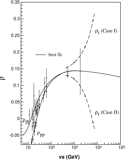
The forward dispersion relations for and scattering represent one of the few general rigorous consequences of local quantum field theory. One tests their validity by measuring , and comparing the results with the calculated obtained from the dispersion relations with as an input. These tests have been carried out at increasing energies for both , and . The highest energy, only, is . The agreement between theory and experiment is good, as can be seen from figure 1.
A measurement of at will explore a short distance domain about which we have little previous knowledge. This is in contrast to the preceeding measurements which dealt with length scales that had already been pre-explored by QED.
However, there is a problem. The particle physics folklore includes statements to the effect that short distance structure shows up first, and in more easily detectable ways, in hard collisions, and not in soft collisions such as forward elastic scattering.
Unfortunately, when statements like the above are repeated for 35 years, people get to be rather sloppy in using them. In this brief talk I will clarify this problem and show that in a domain where the dispersion relations no longer hold, is extremely sensitive to the existence of a fundamental length, , and changes drastically even when .
The dilemma between hard and soft collisions can be clarified as follows. Given some kind of structure at short distance, , we can make the following correct statement:
As we approach the energy region such that is non-negligible, then hard cross-sections will in general show a more detectable and larger change than soft cross-sections.
This statement, though not extremely precise, is in general qualitatively correct. However, if in the same statement we replace cross-sections by amplitudes then the statement is false, as we shall demonstrate by counterexample. Of course when local QFT is valid, then for the forward scattering amplitude, , if does not change much in a certain region so will and because one can use the dispersion relation to get from . But, in a world in which the dispersion relations or QFT fail, as we shall show below can be extremely sensitive to a breakdown in QFT.
The main purpose of this talk is to give a “counterexample” to the statement about soft amplitudes being insensitive to a short distance breakdown in QFT. Indeed, I will show that when traditional QFT is changed by a breakdown in polynomial boundedness, which in many models is the main feature of the existence of a fundamental length, then the phase, , could change by more than a factor of 2 even for energies as low as . This happens without any significant change in or .
Before we present our “counterexample”, we summarize briefly the well established properties of in local QFT. We have the following: i) is analytic in the doubly cut s-plane; ii) is crossing symmetric, relating for to for ; iii) satisfies the optical theorem, ; iv) is polynomially bounded in all directions in the cut complex s-plane,
| (3) |
We have argued in ref. 2, that the most likely property to change is iv), i.e. equation (3). Properties ii) and iii) are on a solid footing. While even if property i), analyticity, fails due to some new complex singularities on the physical sheet, these will not lead to a strong signal except for (new singularities).
The breakdown in iv) replaces equ. (3) by an exponential bound:
| (4) |
In fact we claim more. Namely, that along some complex s direction, grows exponentially like . Note that a behavior of the type , with , is excluded due to some technical mathematical arguments. Hence one goes from behavior to a first order exponential in .
There are several examples which exhibit the behavior (4). These are:
a.) Non-local Potential Scattering
Here one replaces the interaction term in the Schrodinger equation, by a non-local one, i.e.,
| (5) |
where
| (6) |
b.) Some Nonlocal Field Theories.
c.) String-Theory3 (
Once we have exponential behavior in we have a natural way to define a “fundamental length”. Noting that momentum for large , then the we use in the bound to make a dimensionless exponent is by definition our fundamental length. We take the smallest such that for some complex sequence , as , actually grows like .
Our main counterexample is a representative of what happens in non-local potential scattering as defined by equ. (5) and (6). It also mimics the behavior of some non-local field theories, although these admittedly have serious problems.
In non-local potential scattering one can easily prove the analyticity of , but is not polynomially bounded as . However, one can prove that as in all directions . The physical sheet here corresponds to , and is defined in equ.(6).
These facts lead us to the following ansatz:
| (7) |
where is the true amplitude, and is a “false” amplitude defined by (7). The true amplitude satisfies the optical theorem, , but is not necessarily positive. However, by definition it is that is polynomially bounded. Also satisfies the dispersion relations albeit with a non-positive . Finally, has no dispersion relation because of its exponential growth when , and .
At first the ansatz(7) looks like a tautology, or at best a definition of .Nevertheless, because of the special properties of for we can still learn much from this ansatz.
We consider two energy regions. A “low” energy region , and a “transitional” region . We also note the fact that for , is small and decreases logarithmically. At , we have . Given the fact that cosmic ray data tell us that will continue to increase, , the dispersion relation fit shown by the curve in figure 1, will continue to decrease slowly as increases.
We consider the two energy regions separately.
A. Low Energy Region,
In this region, we have
There is no observable difference between the polynomially bounded amplitude and the exponentially bounded one.
B. Transitional Region
Here is small but not negligible,
| (8) |
Note that is still well below .
From the ansatz(7), we obtain
| (9) |
At this stage it is important to remark that the second term in the bracket in (10) is doubly small, is small and . We obtain
| (10) |
To proceed further let us assume that in the transitional region, , a bound almost 2.5 times larger than the value of at . We hasten to add that this assumption is not really needed, but it gives us a quick way to arrive at our result. Later we shall show how one can get the same result without this assumption. We now have,
| (11) |
for . Thus in the transitional region , and hence for and the optical theorem holds for to a very good approximation. But satisfies a dispersion relation, and we can therefore use the approximate derivative form of the dispersion relations4 to get
| (12) |
where is the dispersion relation fit to as the one shown by the continuous curve in figure 1.
The “true” and “false” phases are related by
| (13) |
with . After some simple algebra we get
| (14) |
But in the transitional region. Replacing by in (15) and expanding in powers of , we get
| (15) |
The error, , is determined by
| (16) |
There are two important features of our final result (16) which should be stressed. First, while decreases logarithmically the additional term increases linearly with , and even when it leads to a 75% increase in . The second feature is the fact that appears linearly in (16), unlike the correction to the muon (g-2) in equ. (1) which was , with appearing in the correction. Since is very small, this makes the QED case less sensitive to a fundamental length.
In figure 1 we plot for . The fact that is sensitive is amply demonstrated.
In closing, we explain briefly how our assumption on can be removed. One has to divide the interval, , into small intervals, . Then one carries out the same calculation we did above step by step starting at , and calculating at the next point. At each step one uses the approximation . The result given by equ.(16) remains the same.
There are other examples which lead to a decrease in rather than the increase given by the ansatz (7). For example one could have instead of (7),
| (17) |
This leads to
| (18) |
with the result shown in figure 1 for , and labeled as case II.
Our ansatz is an example of a whole class where one can write , where is an entire function of order 1. All these lead, via similar arguments, to a dramatic change in ,
| (19) |
where .
In conclusion, is extremely sensitive to a short distance breakdown of QFT, and more so if that breakdown is manifested by the failure of polynomial boundedness and its replacement by exponential growth which is order 1 in the variable . Here is the c.m. momentum in forward scattering, and we take, by definition, to be the “fundamental length”.
Strictly within the context of this picture, we can set the following limits on a breakdown in polynomial boundedness:
1.) gives us a lower limit for , .
2.) if redone with smaller errors could improve this bound to ; here .
3.) Agreement between and at LHC could get us .
Acknowledgements
This work was supported in part by the U.S. Department of Energy under grant no. DOE91ER40651 TaskB.
References and Footnotes
[1] T. Kinoshita, Quantum Electrodynamics, T.K. Editor, (World Scientific, 1990), pp. 471. It should be stressed that one should not confuse our here with the limits on the lepton or quark form factors in QCD. In axiomatic QFT even the deuteron, which certainly is composite, has an interpolating field which is strictly causal, i.e. two field operators at x and y commute if , i.e. spacelike. This leads to dispersion relations for forward scattering. If does not satisfy strict causality, this will have little to do with whether or the electron are composite or not.
[2] N.N. Khuri, “Proceedings of Les Recontres de Physiques da la Vallee d’Aoste: Results and Perspectives in Particle Physics” (M. Greco, Ed.), pp 701-708. Editions Frontieres, Gif-sur-Yvette, France, 1994.
[3] D.J. Gross and P. Mende, Nucl. Phys. B303, 407 (l988).
[4] See for example, E. Leader, Phys. Rev. Lett. 59, 1525 (1987).