SISSA 103/95/EP

A New Estimate of $\varepsilon^{\prime}/\varepsilon$

S. Bertolini^†, J.O. Eeg^‡ and M. Fabbrichesi^†

^† INFN, Sezione di Trieste, and
Scuola Internazionale Superiore di Studi Avanzati
via Beirut 4, I-34013 Trieste, Italy.

^‡ Department of Physics, University of Oslo
N-0316 Oslo, Norway.

Abstract

We discuss direct $CP$ violation in the standard model by giving a new estimate of $\varepsilon^{\prime}/\varepsilon$ in kaon decays. Our analysis is based on the evaluation of the hadronic matrix elements of the $\Delta S=1$ effective quark lagrangian by means of the chiral quark model, with the inclusion of meson one-loop renormalization and NLO Wilson coefficients. Our estimate is fully consistent with the $\Delta I=1/2$ selection rule in $K\to\pi\pi$ decays which is well reproduced within the same framework. By varying all parameters in the allowed ranges and, in particular, taking the quark condensate—which is the major source of uncertainty—between $(-200\ {\rm MeV})^{3}$ and $(-280\ {\rm MeV})^{3}$ we find

$$-5.0\times 10^{-3}\ <\varepsilon^{\prime}/\varepsilon<\ 1.4\times 10^{-3}\,.$$

Assuming for the quark condensate the improved PCAC result $\left\langle\bar{q}q\right\rangle=-(221\>\pm 17\ {\rm MeV})^{3}$ and fixing $\Lambda_{\rm QCD}^{(4)}$ to its central value, we find the more restrictive prediction

$$\varepsilon^{\prime}/\varepsilon=(4\pm 5)\,\times\,10^{-4}\ ,$$

where the central value is defined as the average over the allowed values of Im $\lambda_{t}$ in the first and second quadrants. In these estimates the relevant mixing parameter Im $\lambda_{t}$ is self-consistently obtained from $\varepsilon$ and we take $m_{t}^{\rm pole}=180\pm 12$ GeV. Our result is, to a very good approximation, renormalization-scale and $\gamma_{5}$-scheme independent.
SISSA 103/95/EP
November 1995

1 Introduction

The real part of $\varepsilon^{\prime}/\varepsilon$ measures direct $CP$ violation in the decays of a neutral kaon in two pions. It is a fundamental quantity which has justly attracted a great deal of theoretical as well as experimental work. Its determination would answer the question of whether $CP$ violation is present only in the mass matrix of neutral kaons (the superweak scenario) or is instead at work also directly in the decays.

On the experimental front, the present results of CERN (NA31) [2]

$$\mbox{Re}\>\left(\varepsilon^{\prime}/\varepsilon\right)=(23\pm 7)\times 10^{-4}$$ (1.1)

and Fermilab (E731) [3]

$$\mbox{Re}\>\left(\varepsilon^{\prime}/\varepsilon\right)=(7.4\pm 6.0)\times 10^{-4}$$ (1.2)

are tantalizing insofar as the superweak scenario cannot be excluded and the disagreement between the two outcomes still leaves a large uncertainty. The next generation of experiments—presently under way at CERN, Fermilab and DA$\Phi$NE—will improve the sensitiveness to $1\times 10^{-4}$ and hopefully reach a definite result.

On the theoretical side, much has been accomplished, although the intrinsic difficulty of a problem that encompasses scales as different as $m_{t}$ and $m_{\pi}$ weights against any decisive progress in the field.

A fundamental step was recently covered by the Munich [4] and Rome [5] groups who computed the anomalous dimension matrix of the ten relevant operators to the next-to-leading order (NLO) in two $\gamma_{5}$-schemes of dimensional regularization: ’t Hooft-Veltman (HV) and Naive Dimensional Regularization (NDR). This computation has brought the short-distance part of the effective lagrangian under control.

The residual (and, unfortunately, largest) uncertainty is due to the long-distance part of the lagrangian, the computation of which implies evaluating the hadronic matrix elements of the quark operators. It is here that the non-perturbative regime of QCD is necessarily present and our understanding is accordingly blurred.

At present, there exist two complete estimates of such hadronic matrix elements performed by the aforementioned groups, and recently updated in ref. [6] for the lattice (at least for some of the operators), where the value

$$\mbox{Re}\>\left(\varepsilon^{\prime}/\varepsilon\right)=(3.1\pm 2.5\pm 0.3)\times 10^{-4}$$ (1.3)

is found, and ref. [7] for the $1/N_{c}$ approach (for all ten operators) improved by fitting the $\Delta I=1/2$ rule, where $\varepsilon^{\prime}/\varepsilon$ is estimated to be within the range

$$-2.5\times 10^{-4}\leq\mbox{Re}\>\left(\varepsilon^{\prime}/\varepsilon\right)\leq 13.7\times 10^{-4}\,.$$ (1.4)

The smaller error in eq. (1.3) originates in the Gaussian treatment of the uncertainty in the input parameters with respect to the flat 1$\sigma$ error included in eq. (1.4).

Both groups seem to agree on the difficulty of accommodating within the standard model a value substantially larger than $1\times 10^{-3}$. This unexpectedly small value is the result of the cancellation between gluon and electroweak penguin operators [8]. If that is actually the case, it is somewhat disappointing that the presence of direct $CP$ violation in the standard model turns out to be hidden by an accidental cancellation that effectively mimics the superweak scenario.

It seemed to us that a third, independent estimate of $\varepsilon^{\prime}/\varepsilon$ was desirable and we have taken the point of view that a reliable evaluation of the hadronic matrix elements should first provide a consistent picture of kaon physics, starting from the $CP$-conserving amplitudes and, in particular, by reproducing the $\Delta I=1/2$ selection rule, which governs most of these amplitudes as well as the quantity $\varepsilon^{\prime}/\varepsilon$ itself. We also felt that the same evaluation should pay particular attention to the problem of achieving a satisfactory $\gamma_{5}$-scheme and scale independence in the matching between the matrix elements and the Wilson coefficients, the absence of which would undermine any estimate.

In a preliminary work [9], we studied $\varepsilon^{\prime}/\varepsilon$ within the chiral quark model ($\chi$QM) [10] in a toy model that included the leading effect of the two most important operators, and verified that the $\gamma_{5}$-scheme independence could be achieved.

In a recent paper [11], hereafter referred as I, we have completed the study of the hadronic matrix elements of all the ten operator of the $\Delta S=1$ effective quark langrangian by means of the $\chi$QM and verified in [12], hereafter referred as II, that the inclusion of non-perturbative $O(\alpha_{s}N_{c})$ corrections and one-loop meson renormalization provided an improved scale independence and, more importantly, a good fit of the $\Delta I=1/2$ selection rule.

These results put us in the position to provide a new estimate of $\varepsilon^{\prime}/\varepsilon$ that is independent of the existing ones and that contains new features that, in our judgment, makes it more reliable.

We summarize here such features. Our estimate takes advantage, as the existing ones, of

• NLO results for the Wilson coefficients;

• up-to-date analysis of the constraints on the mixing coefficient Im $\lambda_{t}$.

Among the new elements introduced, the most relevant are

• A consistent evaluation of all hadronic matrix elements in the $\chi$QM (including non-perturbative gluon condensate effects) in two schemes of dimensional regularization;

• Inclusion in the $\Delta S=1$ chiral lagrangian of the complete bosonization $O(p^{2})$ of the electroweak operators $Q_{7}$ and $Q_{8}$. Some relevant $O(p^{2})$ terms have been neglected in all previous estimates;

• Inclusion of the meson-loop renormalization and scale dependence of the matrix elements;

• Consistency with the $\Delta I=1/2$ selection rule in kaon decays;

• Matching-scale and $\gamma_{5}$-scheme dependence of the results below the 20% level.

Even though our framework enjoys a high degree of reliability, any estimate of $\varepsilon^{\prime}/\varepsilon$ necessarily suffers of a systematic uncertainty that cannot be easily reduced further. We find that it is mainly parameterized in terms of the value of the quark condensate, the input parameter that dominates penguin-diagram physics. For this reason, we discuss first a inclusive estimate based on a conservative range of $\left\langle\bar{q}q\right\rangle$, as well as the variations of all the other inputs: $m_{t}$, $\mathop{\mbox{Im}}\lambda_{t}$ (which depends, beside $m_{t}$ and $m_{c}$, on $\hat{B}_{K}$ and other mixing angles) and $\Lambda_{\rm QCD}$. Such a procedure provides us with the range of values for $\varepsilon^{\prime}/\varepsilon$ that we consider to be the unbiased theoretical prediction of the standard model. Unfortunately, this range turns out to be rather large, spanning, as it can be seen in the abstract, from $-5\times 10^{-3}$ to $1.4\times 10^{-3}$. On the other hand, it is as small as we can get without making some further assumptions on the input parameters—assumptions that all the other available estimates must make as well.

In order to provide such a more restrictive estimate, we have chosen the improved PCAC prediction for the quark condensate and fixed $\Lambda_{\rm QCD}^{(4)}$ to its central value. This reasonable, but nevertheless arbitrary choice allows us to give the second, and more predictive estimate reported in the abstract. It is the latter that should be compared with the current estimates, while, at the same time, bearing in mind also the former unrestricted range as a realistic measure of our ignorance.

Such uncertainty notwithstanding, we agree in the end with the main point of ref. [6], namely that it is difficult to accommodate within the standard model a value of $\varepsilon^{\prime}/\varepsilon$ larger than $1\times 10^{-3}$. In fact, if our analysis points toward a definite prediction, it points to even smaller values, if not negative ones. This can be understood not so much as a peculiar feature of the $\chi$QM prediction as the neglect in other estimates of a class of contributions in the vacuum saturation approximation (VSA) of the matrix elements of the electroweak operators. This problem is discussed in detail in I. These new contributions are responsible for the onset of the superweak regime for values of $m_{t}$ less than 200 GeV. In our computation, it is the meson renormalization that in the end brings back $\varepsilon^{\prime}/\varepsilon$ around zero or positive values.

The outline of the paper is the following. In section 2 we write the effective quark lagrangian, discuss the short-distance input parameters and give the Wilson coefficients. Section 3 contains a brief discussion of the $\chi$QM evaluation of the hadronic matrix elements and their corresponding meson-loop renormalization. In section 4 we discuss the values of the input parameters and in section 5 the effective factors $B_{i}$’s that give the comparison between the VSA and the $\chi$QM evaluation of the hadronic matrix elements. We begin in section 6 our discussion of $\varepsilon^{\prime}/\varepsilon$ by first studying the $\gamma_{5}$-scheme independence and then the contribution of each operator taken by itself. In section 7, we give our estimate as a function of the most important input parameters in a series of figures and one table. The numerical value of all input parameters are collected in a table in the appendix.

2 The Quark Effective Lagrangian and the NLO Wilson Coefficients

The quark effective lagrangian at a scale $\mu<m_{c}$ can be written as [13]

$${\cal L}_{\Delta S=1} = -\frac{G_{F}}{\sqrt{2}}V_{ud}\,V^{*}_{us}\sum_{i}\Bigl{[}z_{i}(\mu)+\tau y_{i}(\mu)\Bigr{]}Q_{i}(\mu)$$ (2.1)

$$\equiv -\frac{G_{F}}{\sqrt{2}}\sum_{i}C_{i}(\mu)Q_{i}(\mu)\,.$$

The $Q_{i}$ are four-quark operators obtained by integrating out in the standard model the vector bosons and the heavy quarks $t,\,b$ and $c$. A convenient and by now standard basis includes the following ten quark operators:

$$\begin{array}[]{rcl}Q_{1}&=&\left(\overline{s}_{\alpha}u_{\beta}\right)_{\rm V-A}\left(\overline{u}_{\beta}d_{\alpha}\right)_{\rm V-A}\,,\\[4.30554pt] Q_{2}&=&\left(\overline{s}u\right)_{\rm V-A}\left(\overline{u}d\right)_{\rm V-A}\,,\\[4.30554pt] Q_{3,5}&=&\left(\overline{s}d\right)_{\rm V-A}\sum_{q}\left(\overline{q}q\right)_{\rm V\mp A}\,,\\[4.30554pt] Q_{4,6}&=&\left(\overline{s}_{\alpha}d_{\beta}\right)_{\rm V-A}\sum_{q}(\overline{q}_{\beta}q_{\alpha})_{\rm V\mp A}\,,\\[4.30554pt] Q_{7,9}&=&\frac{3}{2}\left(\overline{s}d\right)_{\rm V-A}\sum_{q}\hat{e}_{q}\left(\overline{q}q\right)_{\rm V\pm A}\,,\\[4.30554pt] Q_{8,10}&=&\frac{3}{2}\left(\overline{s}_{\alpha}d_{\beta}\right)_{\rm V-A}\sum_{q}\hat{e}_{q}(\overline{q}_{\beta}q_{\alpha})_{\rm V\pm A}\,,\end{array}$$ (2.2)

where $\alpha$, $\beta$ denote color indices ($\alpha,\beta=1,\ldots,N_{c}$) and $\hat{e}_{q}$ are quark charges. Color indices for the color singlet operators are omitted. The labels $(V\pm A)$ refer to $\gamma_{\mu}(1\pm\gamma_{5})$. We recall that $Q_{1,2}$ stand for the $W$-induced current–current operators, $Q_{3-6}$ for the QCD penguin operators and $Q_{7-10}$ for the electroweak penguin (and box) ones.

The functions $z_{i}(\mu)$ and $y_{i}(\mu)$ are the Wilson coefficients and $V_{ij}$ the Kobayashi-Maskawa (KM) matrix elements; $\tau=-V_{td}V_{ts}^{*}/V_{ud}V_{us}^{*}$. Following the usual parametrization of the KM matrix, in order to determine $\varepsilon^{\prime}/\varepsilon$, we only need the $y_{i}(\mu)$, which control the $CP$-violating part of the amplitudes.

The size of the Wilson coefficients at the hadronic scale ($\sim 1$ GeV) depends on $\alpha_{s}$ and the threshold masses $m_{W}$, $m_{b}$ and $m_{c}$. In addition, the penguin coefficients $y_{i}(\mu)$ depend on the top mass via the initial matching conditions.

The recent determination of the strong coupling at LEP and SLC gives [14]

$$\alpha_{s}(m_{Z})=0.119\pm 0.006\,,$$ (2.3)

which corresponds to

$$\Lambda^{(4)}_{QCD}=350\pm 100\>\mbox{MeV}\,.$$ (2.4)

We will use the range in eq. (2.4) for our numerical estimate of $\varepsilon^{\prime}/\varepsilon$.

For $m_{t}$ we take the value [15]

$$m_{t}^{\rm pole}=180\pm 12\>\>\mbox{GeV}$$ (2.5)

The relation between the pole mass $M$ and the $\overline{\rm MS}$ running mass $\overline{m}(\mu)$ is given at one loop in QCD by [18]:

$$\overline{m}(M)\ =\ {M(q^{2}=M^{2})}\ {\left(1-\frac{4}{3}\frac{\alpha_{s}(M)}{\pi}\right)}\ \ ,$$ (2.6)

For the running top quark mass, in the range of $\alpha_{s}$ considered, we obtain

$$\overline{m}_{t}(m_{t}^{\rm pole})\simeq 172\pm 12\>\>\mbox{GeV}$$ (2.7)

which, using the one-loop running, corresponds to

$$\overline{m}_{t}(m_{W})\simeq 183\pm 14\>\>\mbox{GeV}\,,$$ (2.8)

which is the value to be used as input at the $m_{W}$ scale for the NLO evolution of the Wilson coefficients. In eq. (2.8) we have averaged over the range of $\Lambda^{(4)}_{QCD}$ given in eq. (2.4). We have explicitly checked that taking $\mu=m_{t}^{\rm pole}$ as the initial matching scale in place of $m_{W}$ and using correspondingly $\overline{m}_{t}(m_{t}^{\rm pole})$ the electroweak Wilson coefficients at $\mu=1$ GeV remain stable up to the percent level, while the variation of the relevant gluon penguin coefficients stays below 15%. The stability worsen by keeping the top mass fixed, while varying the matching scale.

For $m_{b}$ we take the value

$$m_{b}^{\rm pole}=4.8\>\>\mbox{GeV}$$ (2.9)

which falls in the range $4.5-4.9$ given in [15], and for $m_{c}$

$$m_{c}^{\rm pole}=1.4\>\>\mbox{GeV}$$ (2.10)

which is in the range $1.2-1.9$ GeV quoted in [15]. These are the quark threshold values we use in evolving the Wilson coefficients down to the 1 GeV scale. We have checked that varying $m_{b}^{\rm pole}$ within the $4.5-4.9$ GeV range affects the final values of the Wilson coefficients at the 0.1% level, while varying the charm pole mass between 1.2 and 1.9 GeV affects the results at the 15% level at most.

Even though not all the operators in eq. (2.2) are independent, this basis is of particular interest for the present numerical analysis because it is that employed for the calculation of the Wilson coefficients to the NLO order in $\alpha_{s}$ and $\alpha_{e}$ [4, 5].

In tables 1 and 2 we give explicitly the Wilson coefficients $y_{i}(\mu)$ of the ten operators at the scale $\mu=1.0$ and 0.8 GeV, respectively, in the HV and NDR schemes. In the $\chi$QM the chiral symmetry breaking scale $\Lambda_{\chi}$ turns out to be about 0.8 GeV. This sets a preferential scale for the matching of the hadronic matrix elements to the Wilson coefficients. We have checked that the QCD perturbative expansion is under control. In fact the difference between LO and NLO results for all physical amplitudes considered—both real and imaginary parts—at $\mu=0.8$ GeV remains always smaller than 30%.

$\Lambda_{QCD}^{(4)}$	250 MeV		350 MeV		450 MeV
$\alpha_{s}(m_{Z})_{\overline{\rm MS}}$	0.113		0.119		0.125
HV
$y_{3}$	$(0.0007)$	$0.0301$	$(0.0007)$	$0.0390$	$(0.0007)$	$0.0509$
$y_{4}$	$(0.0011)$	$-0.0513$	$(0.0012)$	$-0.0610$	$(0.0012)$	$-0.0723$
$y_{5}$	$(-0.0004)$	$0.0137$	$(-0.0004)$	$0.0163$	$(-0.0004)$	$0.0209$
$y_{6}$	$(0.0011)$	$-0.0766$	$(0.0012)$	$-0.103$	$(0.0012)$	$-0.144$
$y_{7}/\alpha$	$(0.172)$	$-0.0115$	$(0.172)$	$-0.0103$	$(0.172)$	$-0.0083$
$y_{8}/\alpha$	$(0)$	$0.167$	$(0)$	$0.230$	$(0)$	$0.328$
$y_{9}/\alpha$	$(-1.19)$	$-1.71$	$(-1.19)$	$-1.83$	$(-1.19)$	$-2.00$
$y_{10}/\alpha$	$(0)$	$0.750$	$(0)$	$0.859$	$(0)$	$1.10$
NDR
$y_{3}$	$(0.0017)$	$0.0268$	$(0.0018)$	$0.0336$	$(0.0018)$	$0.0416$
$y_{4}$	$(-0.0019)$	$-0.0491$	$(-0.0021)$	$-0.0574$	$(-0.0022)$	$-0.0660$
$y_{5}$	$(0.0007)$	$0.0031$	$(0.0007)$	$-0.0028$	$(0.0007)$	$-0.0165$
$y_{6}$	$(-0.0019)$	$-0.0849$	$(-0.0021)$	$-0.119$	$(-0.0022)$	$-0.178$
$y_{7}/\alpha$	$(0.149)$	$-0.0119$	$(0.149)$	$-0.0118$	$(0.136)$	$-0.0127$
$y_{8}/\alpha$	$(0)$	$0.153$	$(0)$	$0.212$	$(0)$	$0.304$
$y_{9}/\alpha$	$(-1.22)$	$-1.71$	$(-1.22)$	$-1.83$	$(-1.22)$	$-1.99$
$y_{10}/\alpha$	$(0)$	$0.674$	$(0)$	$0.843$	$(0)$	$1.07$

Table 1: NLO Wilson coefficients at $\mu=1.0$ GeV for $\overline{m}_{t}(m_{W})=183$ GeV, which corresponds to $m_{t}^{pole}=180$ GeV. The values of the coefficients at $\mu=m_{W}$ are given in parenthesis ($\alpha=1/128$). In addition one has $y_{1,2}(\mu)=0$.

In order to test the $\mu$ independence of $\varepsilon^{\prime}/\varepsilon$ we vary the matching scale between 0.8 and 1.0 GeV, the highest energy up to which we trust the chiral loop corrections computed in I. We find that, in spite of the fact that some of the Wilson coefficients vary in this range by up to 50%, the matching with our matrix elements reduces the $\mu$-dependence in $\varepsilon^{\prime}/\varepsilon$ below 20% in most of the parameter space. We consider this improved stability a success of the approach.

$\Lambda_{QCD}^{(4)}$	250 MeV		350 MeV		450 MeV
$\alpha_{s}(m_{Z})_{\overline{\rm MS}}$	0.113		0.119		0.125
HV
$y_{3}$	$(0.0007)$	$0.0338$	$(0.0007)$	$0.0456$	$(0.0007)$	$0.0602$
$y_{4}$	$(0.0011)$	$-0.0522$	$(0.0012)$	$-0.0626$	$(0.0012)$	$-0.0741$
$y_{5}$	$(-0.0004)$	$0.0140$	$(-0.0004)$	$0.0192$	$(-0.0004)$	$0.0397$
$y_{6}$	$(0.0011)$	$-0.0904$	$(0.0012)$	$-0.137$	$(0.0012)$	$-0.242$
$y_{7}/\alpha$	$(0.172)$	$-0.0131$	$(0.172)$	$-0.0111$	$(0.172)$	$-0.0039$
$y_{8}/\alpha$	$(0)$	$0.209$	$(0)$	$0.327$	$(0)$	$0.583$
$y_{9}/\alpha$	$(-1.19)$	$-1.82$	$(-1.19)$	$-2.04$	$(-1.19)$	$-2.45$
$y_{10}/\alpha$	$(0)$	$0.835$	$(0)$	$1.14$	$(0)$	$1.66$
NDR
$y_{3}$	$(0.0017)$	$0.0294$	$(0.0018)$	$0.0373$	$(0.0018)$	$0.0422$
$y_{4}$	$(-0.0019)$	$-0.0493$	$(-0.0021)$	$-0.0569$	$(-0.0022)$	$-0.0603$
$y_{5}$	$(0.0007)$	$-0.0014$	$(0.0007)$	$-0.0167$	$(0.0007)$	$-0.0708$
$y_{6}$	$(-0.0019)$	$-0.104$	$(-0.0021)$	$-0.171$	$(-0.0022)$	$-0.353$
$y_{7}/\alpha$	$(0.149)$	$-0.0138$	$(0.149)$	$-0.0156$	$(0.149)$	$-0.0274$
$y_{8}/\alpha$	$(0)$	$0.189$	$(0)$	$0.294$	$(0)$	$0.511$
$y_{9}/\alpha$	$(-1.22)$	$-1.81$	$(-1.22)$	$-2.03$	$(-1.22)$	$-2.42$
$y_{10}/\alpha$	$(0)$	$0.819$	$(0)$	$1.11$	$(0)$	$1.60$

Table 2: Same as in Table 1 at $\mu=0.8$ GeV.

3 The Hadronic Matrix Elements

In paper I we have computed all hadronic matrix elements of the effective quark operators in eq. (2.2) in the framework of the $\chi$QM. The matrix elements are obtained by the integration of the constituent quarks by means of dimensional regularization. The loop integration leads to results that depend on the scheme employed to deal with $\gamma_{5}$ but are scale independent. The renormalization-scale dependence is introduced in our approach by the meson-loop renormalization of the amplitudes, as explained in I. The meson-loop corrections together with the gluon-condensate contributions are the most relevant ingredients in reproducing the $\Delta I=1/2$ selection rule in $K\to\pi\pi$ decays, (as discussed in II).

The $\chi$QM results are expressed in a double power expansion on $M^{2}/\Lambda_{\chi}^{2}$ and $p^{2}/\Lambda_{\chi}^{2}$, where $M$ is a dimensionful parameter of the model which is not determined (generically, it can be interpreted as the constituent quark mass in mesons) and $p$ is a typical external momentum.

The value of $M$ is constrained [16] by experimental data on the decay of $\pi^{0}$ and $\eta$ to be

$$M=223\pm 9\>\mbox{MeV}$$ (3.1)

(and $M=243\pm 9$ MeV if higher order corrections are included). The value of

$$M=m_{\rho}/\sqrt{12}\simeq 222\ \mbox{MeV}$$ (3.2)

is found by vector-meson-dominance estimates. Finally, in a recent fit of all input parameteres of the extended Nambu-Jona-Lasinio model [17], it was found a value of

$$M\simeq 200\>\mbox{MeV}\,.$$ (3.3)

While we could simply take these values and thus make the $\chi$QM predictive, our approach also allows for a self-consistent determination of a range for $M$ that can be compared to the above values.

The idea is that in physical observables the $\gamma_{5}$-scheme and $\mu$-dependences of the matrix elements should balance the corresponding dependences of the NLO Wilson coefficients . In I we have constructed the complete $O(p^{2})$ chiral representation of the lagrangian in eq. (2.1), where the local quark operator $Q_{i}$ is represented by a linear combination of bosonic operators $B_{\alpha}$, namely $Q_{i}\to\sum_{\alpha}G_{\alpha}(Q_{i})B_{\alpha}$. The effective quark lagrangian is therefore replaced by the following chiral representation

$${\cal L}^{\Delta S=1}_{\chi}=-\frac{G_{F}}{\sqrt{2}}\ \sum_{i,\alpha}\ C_{i}(\mu)\ G_{\alpha}(Q_{i})\ B_{\alpha}\,.$$ (3.4)

As mentioned above, and discussed at lenght in I, the chiral coefficients $G_{\alpha}$ determined via the $\chi$QM approach are $\gamma_{5}$-scheme dependent. While the $\gamma_{5}$-scheme dependence arises in the $\chi$QM from the integration of the chiral fermions, the explicit $\mu$-dependence is entirely due to the chiral loop renormalization of the matrix elements:

$$\left\langle b|{\cal L}^{\Delta S=1}_{\chi}|a\right\rangle=-\frac{G_{F}}{\sqrt{2}}\ \sum_{i,\alpha}\ C_{i}(\mu_{SD})\ G_{\alpha}(Q_{i})\ \left\langle b|B_{\alpha}|a\right\rangle(\mu_{LD})\,,$$ (3.5)

where we have labeled by $a$ and $b$ the initial and final bosonic states. We remark that in our approach the $\mu$-dependence of the chiral loops is not cancelled by higher order counterterms, as it is usually required in the strong chiral lagrangian.

The renormalization scale dependence is therefore determined order by order in the energy expansion of the chiral lagrangian. In this respect there is no direct counterpart to the expansion in strong and electromagnetic couplings on which the short-distance analysis is based and, accordingly, we refer to the explicit $\mu$-dependence in the matrix elements as to the long-distance (LD) or “non-perturbative” scale dependence. A purely perturbative renormalization scale dependence is introduced in the matrix elements by the NLO running of the quark condensate, which we include whenever a comparison between values at different scales is required. Otherwise, quark and gluon condensates are considered in our approach as phenomenological parameters.

Our aim is to test whether the estimate of observables is consistently improved by matching the “long-distance” $\gamma_{5}$-scheme and $\mu$ dependences so obtained with those present in the short-distance analysis (in particular we identify $\mu_{SD}$ with $\mu_{LD}$). Whether and to what extent such an improvement is reproduced for many observables and for a consistent set of parameters, might tell us how well low-energy QCD is modelled in the $\chi$QM-chiral lagrangian approach that we have devised.

In II, we have shown that minimizing the $\gamma_{5}$-scheme dependence of the physical isospin $I=0$ and 2 amplitudes determines a range for the parameter $M$ between 160 and 220 MeV. In II, it was also found that the $\mu$ dependence induced by the Wilson coefficients is substantially reduced by that of the hadronic matrix elements.

These issues become crucial for $\varepsilon^{\prime}/\varepsilon$ where the $\gamma_{5}$-scheme dependence induced by the Wilson coefficients determines an uncertainty as large as 80% when using the $1/N_{c}$ hadronic matrix elements (see for instance ref. [4]) which are scheme independent.

In the following, for the reader’s convenience, we report from I the expressions for the isospin amplitudes for all ten operators in eq. (2.2):

$$\langle Q_{i}\rangle_{0,2}\equiv\langle 2\pi,I=0,2|Q_{i}|K^{0}\rangle\,.$$ (3.6)

The corresponding one-loop meson corrections are denoted by $a_{0,2}(Q_{i})$. The Clebsh-Gordan coefficients for the isospin projections can be found in I.

For the HV case we obtain:

$$\langle Q_{1}\rangle_{0} = \frac{1}{3}X\left[-1+\frac{2}{N_{c}}\left(1-\delta_{\left\langle GG\right\rangle}\right)\right]+a_{0}(Q_{1})$$ (3.7)

$$\langle Q_{1}\rangle_{2} = \frac{\sqrt{2}}{3}X\left[1+\frac{1}{N_{c}}\left(1-\delta_{\left\langle GG\right\rangle}\right)\right]+a_{2}(Q_{1})$$ (3.8)

$$\langle Q_{2}\rangle_{0} = \frac{1}{3}X\left[2-\frac{1}{N_{c}}\left(1-\delta_{\left\langle GG\right\rangle}\right)\right]+a_{0}(Q_{2})$$ (3.9)

$$\langle Q_{2}\rangle_{2} = \frac{\sqrt{2}}{3}X\left[1+\frac{1}{N_{c}}\left(1-\delta_{\left\langle GG\right\rangle}\right)\right]+a_{2}(Q_{2})$$ (3.10)

$$\langle Q_{3}\rangle_{0} = \frac{1}{N_{c}}X\left(1-\delta_{\left\langle GG\right\rangle}\right)+a_{0}(Q_{3})$$ (3.11)

$$\langle Q_{4}\rangle_{0} = X+a_{0}(Q_{4})$$ (3.12)

$$\langle Q_{5}\rangle_{0} = \frac{2}{N_{c}}\,\frac{\langle\bar{q}q\rangle}{Mf_{\pi}^{2}}\,X^{\prime}+a_{0}(Q_{5})$$ (3.13)

$$\langle Q_{6}\rangle_{0} = 2\,\frac{\langle\bar{q}q\rangle}{Mf_{\pi}^{2}}\,X^{\prime}+a_{0}(Q_{6})$$ (3.14)

$$\langle Q_{7}\rangle_{0} = \frac{2\sqrt{3}}{N_{c}}\,\frac{\langle\bar{q}q\rangle^{2}}{f_{\pi}^{3}}-\frac{1}{N_{c}}\,\frac{\langle\bar{q}q\rangle}{Mf_{\pi}^{2}}\,X^{\prime}$$ (3.15)

$$-\frac{2}{N_{c}}\frac{\left\langle\bar{q}q\right\rangle}{Mf_{\pi}^{2}}\ Y+\frac{1}{2}X+a_{0}(Q_{7})$$

$$\langle Q_{7}\rangle_{2} = \sqrt{6}\,\frac{\langle\bar{q}q\rangle^{2}}{f_{\pi}^{3}}\frac{1}{N_{c}}-\frac{\sqrt{2}}{N_{c}}\frac{\left\langle\bar{q}q\right\rangle}{Mf_{\pi}^{2}}\ Y-\frac{\sqrt{2}}{2}X+a_{2}(Q_{7})$$ (3.16)

$$\langle Q_{8}\rangle_{0} = 2\,\sqrt{3}\,\frac{\langle\bar{q}q\rangle^{2}}{f_{\pi}^{3}}-\frac{\langle\bar{q}q\rangle}{Mf_{\pi}^{2}}\,X^{\prime}$$ (3.17)

$$-2\,\frac{\left\langle\bar{q}q\right\rangle}{Mf_{\pi}^{2}}\ Y+\frac{1}{2N_{c}}X\left(1+\delta_{\left\langle GG\right\rangle}\right)+a_{0}(Q_{8})$$

$$\langle Q_{8}\rangle_{2} = \sqrt{6}\,\frac{\langle\bar{q}q\rangle^{2}}{f_{\pi}^{3}}-\sqrt{2}\frac{\left\langle\bar{q}q\right\rangle}{Mf_{\pi}^{2}}\ Y-\frac{\sqrt{2}}{2N_{c}}X\left(1+\delta_{\left\langle GG\right\rangle}\right)+a_{2}(Q_{8})$$ (3.18)

$$\langle Q_{9}\rangle_{0} = -\frac{1}{2}X\left[1-\frac{1}{N_{c}}\left(1-\delta_{\left\langle GG\right\rangle}\right)\right]+a_{0}(Q_{9})$$ (3.19)

$$\langle Q_{9}\rangle_{2} = \frac{\sqrt{2}}{2}X\left[1+\frac{1}{N_{c}}\left(1-\delta_{\left\langle GG\right\rangle}\right)\right]+a_{2}(Q_{9})$$ (3.20)

$$\langle Q_{10}\rangle_{0} = \frac{1}{2}X\left[1-\frac{1}{N_{c}}\left(1-\delta_{\left\langle GG\right\rangle}\right)\right]+a_{0}(Q_{10})$$ (3.21)

$$\langle Q_{10}\rangle_{2} = \frac{\sqrt{2}}{2}X\left[1+\frac{1}{N_{c}}\left(1-\delta_{\left\langle GG\right\rangle}\right)\right]+a_{2}(Q_{10})\,.$$ (3.22)

where

$$X\equiv\sqrt{3}f_{\pi}\left(m_{K}^{2}-m_{\pi}^{2}\right)\ ,\quad\quad X^{\prime}=X\left(1-6\,\frac{M^{2}}{\Lambda_{\chi}^{2}}\right)$$ (3.23)

and

$$Y\equiv\sqrt{3}f_{\pi}\left[m_{\pi}^{2}+3\ m_{K}^{2}\frac{M^{2}}{\Lambda^{2}_{\chi}}\right]\ ;$$ (3.24)

$\delta_{\left\langle GG\right\rangle}$ is given by

$$\delta_{\langle GG\rangle}=\frac{N_{c}}{2}\frac{\langle\alpha_{s}GG/\pi\rangle}{16\pi^{2}f^{4}}\,.$$ (3.25)

It is (3.25) that parameterizes the non-perturbative part of the computation by the contribution of the gluon condensate $\langle\alpha_{s}GG/\pi\rangle$, as discussed in I.

The renormalization of $f$ is taken into account by replacing $f$ with the one-loop parameter $f_{1}$ in the tree-level amplitudes, which amounts to replacing $1/f^{3}$ with $1/f^{3}_{\pi}$ multiplied by

$$1+3\ \frac{f_{\pi}-f_{1}}{f_{\pi}}\simeq 1.18\,.$$ (3.26)

In the NDR case we find:

$$\langle Q_{1}\rangle_{0} = \frac{1}{3}X\left[-1+\frac{2}{N_{c}}\left(1-\delta_{\left\langle GG\right\rangle}\right)\right]+a_{0}(Q_{1})$$ (3.27)

$$\langle Q_{1}\rangle_{2} = \frac{\sqrt{2}}{3}X\left[1+\frac{1}{N_{c}}\left(1-\delta_{\left\langle GG\right\rangle}\right)\right]+a_{2}(Q_{1})$$ (3.28)

$$\langle Q_{2}\rangle_{0} = \frac{1}{3}X\left[2-\frac{1}{N_{c}}\left(1-\delta_{\left\langle GG\right\rangle}\right)\right]+a_{0}(Q_{2})$$ (3.29)

$$\langle Q_{2}\rangle_{2} = \frac{\sqrt{2}}{3}X\left[1+\frac{1}{N_{c}}\left(1-\delta_{\left\langle GG\right\rangle}\right)\right]+a_{2}(Q_{2})$$ (3.30)

$$\langle Q_{3}\rangle_{0} = \frac{1}{N_{c}}\left(X^{\prime}-\delta_{\left\langle GG\right\rangle}X\right)+a_{0}(Q_{3})$$ (3.31)

$$\langle Q_{4}\rangle_{0} = X^{\prime}+a_{0}(Q_{4})$$ (3.32)

$$\langle Q_{5}\rangle_{0} = \frac{2}{N_{c}}\,\frac{\langle\bar{q}q\rangle}{Mf_{\pi}^{2}}\,X^{\prime\prime}+a_{0}(Q_{5})$$ (3.33)

$$\langle Q_{6}\rangle_{0} = 2\,\frac{\langle\bar{q}q\rangle}{Mf_{\pi}^{2}}\,X^{\prime\prime}+a_{0}(Q_{6})$$ (3.34)

$$\langle Q_{7}\rangle_{0} = \frac{2\sqrt{3}}{N_{c}}\,\frac{\langle\bar{q}q\rangle^{2}}{f_{\pi}^{3}}\left(1-3\frac{M^{3}f_{\pi}^{2}}{\langle\bar{q}q\rangle\Lambda_{\chi}^{2}}\right)-\frac{1}{N_{c}}\frac{\langle\bar{q}q\rangle}{Mf_{\pi}^{2}}\,X^{\prime\prime}$$ (3.35)

$$-\frac{2}{N_{c}}\frac{\left\langle\bar{q}q\right\rangle}{Mf_{\pi}^{2}}\ Y^{\prime}+\frac{1}{2}X+a_{0}(Q_{7})$$

$$\langle Q_{7}\rangle_{2} = \frac{1}{N_{c}}\sqrt{6}\,\frac{\langle\bar{q}q\rangle^{2}}{f_{\pi}^{3}}\left(1-3\frac{M^{3}f_{\pi}^{2}}{\langle\bar{q}q\rangle\Lambda_{\chi}^{2}}\right)$$ (3.36)

$$-\frac{\sqrt{2}}{N_{c}}\frac{\left\langle\bar{q}q\right\rangle}{Mf_{\pi}^{2}}\ Y^{\prime}-\frac{\sqrt{2}}{2}X+a_{2}(Q_{7})$$

$$\langle Q_{8}\rangle_{0} = 2\sqrt{3}\,\frac{\langle\bar{q}q\rangle^{2}}{f_{\pi}^{3}}\left(1-3\frac{M^{3}f_{\pi}^{2}}{\langle\bar{q}q\rangle\Lambda_{\chi}^{2}}\right)-\frac{\langle\bar{q}q\rangle}{Mf_{\pi}^{2}}\,X^{\prime\prime}$$ (3.37)

$$-2\,\frac{\left\langle\bar{q}q\right\rangle}{Mf_{\pi}^{2}}\ Y^{\prime}\>+\frac{1}{2N_{c}}X\left(1+\delta_{\left\langle GG\right\rangle}\right)+\>a_{0}(Q_{8})$$

$$\langle Q_{8}\rangle_{2} = \sqrt{6}\,\frac{\langle\bar{q}q\rangle^{2}}{f_{\pi}^{3}}\left(1-3\frac{M^{3}f_{\pi}^{2}}{\langle\bar{q}q\rangle\Lambda_{\chi}^{2}}\right)$$ (3.38)

$$-\sqrt{2}\frac{\left\langle\bar{q}q\right\rangle}{Mf_{\pi}^{2}}\ Y^{\prime}-\frac{\sqrt{2}}{2N_{c}}X\left(1+\delta_{\left\langle GG\right\rangle}\right)\>+a_{2}(Q_{8})$$

$$\langle Q_{9}\rangle_{0} = -\frac{1}{2}\left[X-\frac{1}{N_{c}}\left(2X-X^{\prime}-\delta_{\left\langle GG\right\rangle}X\right)\right]+a_{0}(Q_{9})$$ (3.39)

$$\langle Q_{9}\rangle_{2} = \frac{\sqrt{2}}{2}X\left[1+\frac{1}{N_{c}}\left(1-\delta_{\left\langle GG\right\rangle}\right)\right]+a_{2}(Q_{9})$$ (3.40)

$$\langle Q_{10}\rangle_{0} = \frac{1}{2}\left[2X-X^{\prime}-\frac{1}{N_{c}}\left(1-\delta_{\left\langle GG\right\rangle}\right)X\right]+a_{0}(Q_{10})$$ (3.41)

$$\langle Q_{10}\rangle_{2} = \frac{\sqrt{2}}{2}X\left[1+\frac{1}{N_{c}}\left(1-\delta_{\left\langle GG\right\rangle}\right)\right]+a_{2}(Q_{10})\,.$$ (3.42)

where

$$X^{\prime\prime}=X\left(1-9\ \frac{M^{2}}{\Lambda_{\chi}^{2}}\right)\,,\quad Y^{\prime}\equiv\sqrt{3}f_{\pi}\left[m_{\pi}^{2}+3\ \left(m_{K}^{2}-m_{\pi}^{2}\right)\frac{M^{2}}{\Lambda^{2}_{\chi}}\right]\ .$$ (3.43)

$\langle Q_{i}\rangle_{2}=0$ for $i=3,4,5,6$ in both schemes.

Of particular interest are the matrix elements $\langle Q_{6}\rangle_{0}$ and $\langle Q_{8}\rangle_{2}$ which dominate any estimate of $\varepsilon^{\prime}/\varepsilon$; their leading effect was included in the toy model of ref. [9].

The most striking feature concerning the gluon-penguin operators is the linear dependence on the quark condensate that is found in the $\chi$QM in contrast to the quadratic one of the VSA. This difference explains the different weight that these operators have in the two models.

Concerning the electroweak-penguin operators, as discussed in I, the terms proportional to $Y$—so far neglected in all estimates—give an important contribution that makes the electroweak-penguin operators larger and, accordingly, the cancellation between electroweak and gluon penguins effective even for the present values of $m_{t}$. We shall come back to this point in section 5.

4 The Input Parameters

The quark and the gluon condensates are two input parameters of our computation. As discussed in I, their phenomenological determination is a complicated question (they parameterize the genuine non-perturbative part of the computation) and the literature offers different estimates.

For guidance, we identify the condensates entering our computation with those obtained by fitting the experimental data by means of the QCD sum rules (QCD–SR) or lattice computations.

A review of recent determinations of these parameters, together with a justification of the range below, is given in I. Here we only report the ranges that we will explore in our numerical analysis.

For the gluon condensate, we take the scale independent range

$$\langle\frac{\alpha_{s}}{\pi}GG\rangle=(376\pm 47\>\mbox{MeV})^{4}\,,$$ (4.1)

which encompasses the results of recent QCD-SR analysis [19]. While this is a crucial input parameter in the physics of the $\Delta I=1/2$ rule (see II), it plays only a minor role in a penguin-dominated quantity like $\varepsilon^{\prime}/\varepsilon$.

For the quark condensate, we consider the range

$$-(200\>\mbox{MeV})^{3}\leq\left\langle\bar{q}q\right\rangle\leq-(280\>\mbox{MeV})^{3}$$ (4.2)

which includes the central values and the errors of the QCD-SR [20] and lattice estimates [22].

The rather conservative range (4.2) is the one advocated in I. In II it is shown that the $\Delta I=1/2$ selection rule seems to prefer the upper half of this range.

For comparison, in most estimates of $\varepsilon^{\prime}/\varepsilon$ the PCAC value

$$\left\langle\bar{q}q\right\rangle(\mu)=-\frac{f_{K}^{2}m_{K}^{2}(1-\delta_{K})}{\overline{m}_{s}(\mu)+\overline{m}_{d}(\mu)}\,,$$ (4.3)

is taken (with $\delta_{K}$ equal to zero) and the error range is that of the determination of $m_{s}$ [23]:

$$\overline{m}_{s}(1\>{\rm GeV})=178\pm 18\>{\rm MeV}\,.$$ (4.4)

This choice gives a quark condensate of

$$\left\langle\bar{q}q\right\rangle=-(261\pm 9\>\mbox{MeV})^{3}$$ (4.5)

at $\mu=1.0$ GeV that corresponds, via NLO renormalization at fixed $\Lambda_{\rm QCD}^{(4)}=350$ MeV, to

$$\left\langle\bar{q}q\right\rangle=-(244\pm 9\>\mbox{MeV})^{3}$$ (4.6)

at the matching scale of $\mu=0.8$ GeV. The quark condensate in (4.6) has an uncertainty of only 9 MeV, that is perhaps too small a range to account for the actual uncertainty. For instance, if the QCD-SR improved estimate [21]

$$\delta_{K}=0.34^{+0.23}_{-0.17}$$ (4.7)

is taken into account, the range (at $\mu=1$ GeV) to be explored becomes comparable to that of (4.2):

$$-(183\>\mbox{MeV})^{3}\leq\left\langle\bar{q}q\right\rangle\leq-(256\>\mbox{MeV})^{3}\,,$$ (4.8)

with a central value much smaller than in (4.6).

The range (4.8) is consistent with what one finds by the same PCAC value as in (4.3) but with $f_{K}$ and $m_{K}$ replaced by, respectively, $f_{\pi}$ and $m_{\pi}$, and $\overline{m}_{s}(\mu)+\overline{m}_{d}(\mu)$ by

$$\overline{m}_{u}(1\>{\rm GeV})+\overline{m}_{d}(1\>{\rm GeV})=12\pm 2.5\>{\rm MeV}\,,$$ (4.9)

as given in  [24]. By means of the latter, taken at $\mu=0.8$ GeV, we find

$$\left\langle\bar{q}q\right\rangle=\left(-221\pm 17\>\>\>{\rm MeV}\right)^{3}\,.$$ (4.10)

The range (4.10) suffers of a larger error with respect to that of (4.6), which however does not take into account (4.7) and, accordingly, the much broader range (4.8) which is more realistic.

Because of such uncertainties, we will consider in section 7 two possible ranges for the quark condensate: the range (4.2) for our most conservative estimate and the improved PCAC result (4.10) for a second, more restrictive one. As discussed in the introduction, these two ranges complete each other in providing, at the same time, a definite prediction and a gauge of the overall uncertainty of the prediction itself.

In section 7, in order to make the comparison to other estimates easier, we will also give our result for the range (4.6).

5 The $B_{i}$ Factors

Let us introduce the effective factors

$$B_{i}^{(0,2)}\equiv\frac{\langle Q_{i}\rangle_{0,2}^{\chi{\rm QM}}}{\langle Q_{i}\rangle_{0,2}^{\rm VSA}}\,,$$ (5.1)

which give the ratios between our hadronic matrix elements and those of the VSA. They are a useful way of comparing different evaluations.

In table 3, we collect the $B_{i}$ factors for the ten operators. The values of the $B_{i}$ depend on the scale at which the matrix elements are evaluated, the input parameters and $M$; moreover, in the $\chi$QM they depend on the $\gamma_{5}$-scheme employed. We have given in table 3 a representative example of their values and variations.

The values of $B_{1}^{(0)}$ and $B_{2}^{(0)}$ show that the corresponding hadronic matrix elements in the $\chi$QM are, once non-factorizable contributions and meson renormalization have been included, respectively about ten and three times larger than their VSA values. At the same time, $B_{1}^{(2)}$ and $B_{2}^{(2)}$ turn out to be at most half of what found in the VSA (for the starred entries see the comment at the end of the section). These features make it possible for the selection rule to be reproduced in the $\chi$QM, as extensively discussed in II.

For comparison, in the $1/N_{c}$ approach of ref. [25], the inclusion of meson-loop renormalization through a cutoff regularization, leads, at the scale of 1 GeV, to $B_{1}^{(0)}=5.2$, $B_{2}^{(0)}=2.2$ and $B_{1}^{(2)}=B_{2}^{(2)}=0.55$, a result that is not sufficient to reproduce the $\Delta I=1/2$ rule. The similarity of the HV values $B_{1}^{(2)}=B_{2}^{(2)}=0.55$ obtained in the $\chi$QM with the corresponding $1/N_{c}$ results is remarkable, and yet a numerical coincidence, since the suppression originates from gluon condensate corrections in the $\chi$QM, whereas it is the effect of the meson loop renormalization (regularized via explicit cut-off) in the analysis of ref. [25].

The values of the penguin matrix elements $\left\langle Q_{3}\right\rangle$ and $\left\langle Q_{4}\right\rangle$ in the $\chi$QM lead to rather large $B_{i}$ factors. In the case of $Q_{3}$, the $\chi$QM result has the opposite sign of the VSA result and $B_{3}$ is negative. This is the effect of the large non-perturbative gluon correction.

Regarding the gluon penguin operator $Q_{6}$ (and $Q_{5}$), we find that the $\chi$QM gives a result consistent with the VSA (and the $1/N_{c}$ approach), $B_{6}$ ($B_{5}$) being approximately equal to two for small values of the quark condensate and one-half at larger values. It is the quadratic dependence (to be contrasted to the linear dependence in the $\chi$QM) of the VSA matrix element for the penguin operators that it responsible for the different weight of these operators at different values of the quark condensate.

	HV		NDR
	$\mu=0.8$ GeV	$\mu=1.0$ GeV	$\mu=0.8$ GeV	$\mu=1.0$ GeV
$B^{(0)}_{1}$	10.6	11.1	10.6	11.1
$B^{(0)}_{2}$	2.8	3.0	2.8	3.0
$B^{(2)}_{1}$	0.52	0.55	0.52	0.55
$B^{(2)}_{2}$	0.52	0.55	0.52	0.55
$B_{3}$	$-2.9$	$-3.0$	$-3.7$	$-3.9$
$B_{4}$	1.8	1.9	1.0	1.1
$B_{5}=B_{6}$	$1.7\div 0.61$	$1.8\div 0.64$	$1.0\div 0.38$	$1.1\div 0.40$
$B_{7}^{(0)}$	$3.0\div 2.2$	$3.3\div 2.4$	$2.9\div 2.2$	$3.2\div 2.3$
$B_{8}^{(0)}$	$3.3\div 2.2$	$3.6\div 2.4$	$3.2\div 2.2$	$3.5\div 2.4$
$B_{9}^{(0)}$	3.9	4.0	3.5	3.6
$B_{10}^{(0)}$	4.4	4.7	5.6	5.9
$B_{7}^{(2)}$	$2.7\div 1.5$	$3.0\div 1.5$	$2.7\div 1.4$	$2.9\div 1.5$
$B_{8}^{(2)}$	$2.1\div 1.4$	$2.3\div 1.5$	$2.1\div 1.4$	$2.3\div 1.5$
$B_{9}^{(2)}$	0.52	0.55	0.52	0.55
$B_{10}^{(2)}$	0.52	0.55	0.52	0.55

Table 3: The $B_{i}$ factors in the $\chi$QM (including meson-loop renormalizations) at two different scales: $\mu$ = 0.8 and 1.0 GeV and in the two $\gamma_{5}$-schemes. We have taken the gluon condensate at the central value of eq. (4.1), while the range given for $B_{5-8}$ corresponds to varying the quark condensate according to eq. (4.2). The results shown are given for $M=220$ MeV.

The lattice estimate at $\mu=2$ GeV for these operators gives $B_{5}=B_{6}=1.0\pm 0.2$ [6]. A direct comparison in this case is not possible.

The electroweak $B_{i}$ factors are all larger in the $\chi$QM than in the VSA, except for $B_{9,10}^{(2)}$ that are about 1/2 in the HV and about 0.4 in the NDR scheme. For comparison, the lattice estimate at $\mu=2$ GeV in this case yields $B_{7,8}^{(2)}=1.0\pm 0.2$ and $B_{9}^{(2)}=0.62\pm 0.10$ [6].

The most relevant result for $\varepsilon^{\prime}/\varepsilon$ is the value of $B_{8}^{(2)}$ which ranges from 1.5 to 2 times that of the VSA. This increase is due to two independent reasons. On the one hand, we found two new terms in the chiral lagrangian that have not been included so far in the VSA estimate of the matrix elements. The chiral coefficients of these terms are computed in the $\chi$QM approach—as discussed in detail in I. It is an open question how they can be determined in the VSA framework.

From this point of view, what we have referred to as VSA—and used in table 3 as normalization for the $Q_{7,8}$ operators—is not the complete VSA result. The inclusion of the new terms amounts up to a 60% increase of $B_{7,8}^{(2)}$ for small values of $\left\langle\bar{q}q\right\rangle$ in the chosen range and down to about 10% for large values; smaller effects are found in the case of $B_{7,8}^{(0)}$. On the other hand, the meson-loop renormalization associated with the new chiral terms is large (see I) and adds up to reproduce the results shown in table 3. The increase in importance of the operator $Q_{8}$ with respect to $Q_{6}$ turns into a more effective cancellation between the two operators for large values of the quark condensate while at smaller values the gluon penguin contribution prevails.

The relations $B_{9}^{(2)}=B_{2}^{(2)}$, $B_{10}^{(2)}=B_{1}^{(2)}$ and $B_{1}^{(2)}=B_{2}^{(2)}$ hold true in both $\gamma_{5}$-schemes. These relationships are a reminiscent of those among the operators—which are preserved by gluon corrections and meson renormalization.

6 Studying $\varepsilon^{\prime}/\varepsilon$ in the $\chi$QM

The quantity $\varepsilon^{\prime}/\varepsilon$ can be written as

$$\frac{\varepsilon^{\prime}}{\varepsilon}=\frac{G_{F}\omega}{2\left|\epsilon\right|\mathop{\mbox{Re}}{A_{0}}}\>\mbox{Im}\,\lambda_{t}\>\>\left[\Pi_{0}-\frac{1}{\omega}\>\Pi_{2}\right]\,,$$ (6.1)

where, referring to the $\Delta S=1$ quark lagrangian of eq. (2.1),

$$\Pi_{0} = \sum_{i}y_{i}\,\langle Q_{i}\rangle_{0}$$ (6.2)

$$\Pi_{2} = \sum_{i}y_{i}\,\langle Q_{i}\rangle_{2}+\omega\>\sum_{i}y_{i}\,\langle Q_{i}\rangle_{0}\>\Omega_{\eta+\eta^{\prime}}\ ,$$ (6.3)

and

$$\mbox{Im}\,\lambda_{t}\equiv\mathop{\mbox{Im}}V_{td}V^{*}_{ts}\,.$$ (6.4)

The quantity $\Omega_{\eta+\eta^{\prime}}$ includes the effect of the isospin-breaking mixing between $\pi^{0}$ and the etas.

Since Im $\lambda_{u}=0$ according to the standard conventions, the short-distance component of $\varepsilon^{\prime}/\varepsilon$ is determined by the Wilson coefficients $y_{i}$. Following the approach of ref. [4], $y_{1}(\mu)=$ $y_{2}(\mu)=0$. As a consequence, the matrix elements of $Q_{1,2}$ do not directly enter the determination of $\varepsilon^{\prime}/\varepsilon$. On the other hand, in the HV scheme the matrix elements of $Q_{4}$ $Q_{9}$ and $Q_{10}$ can be expressed in terms of those of $Q_{1,2}$ and $Q_{3}$. The work of ref. [4] has taken advantage of this fact to determine some of the penguin matrix elements, after imposing the $\Delta I=1/2$ rule. The $\chi$QM determination of $\left\langle Q_{1,2,3}\right\rangle_{0}$ gives for $\left\langle Q_{4}\right\rangle_{0}$ a result that differs substantially from that used in ref. [4], as we discuss at the end of section 6.3.

We take, as input values for the relevant quantities, the central values given in appendix. We thus have

$$\frac{G_{F}\omega}{2\left|\epsilon\right|\mathop{\mbox{Re}}{A_{0}}}\simeq 349\ \mbox{GeV}^{-3},\qquad\omega=1/22.2\ ,\qquad\Omega_{\eta+\eta^{\prime}}=0.25\ .$$ (6.5)

The large value in eq. (6.5) for $1/\omega$ comes from the $\Delta I=1/2$ selection rule. In II we have shown that such a rule is well reproduced by the $\chi$QM evaluation of the hadronic matrix elements. As the precise values of $\mathop{\mbox{Re}}A_{0}$ and $\omega$ depend on the choice of the input parameters and of $M$—the selection rule being satisfied within a 20% approximation—we have taken the corresponding experimental values. Similarly, the value taken for $\varepsilon$ is the experimental one.

6.1 The Mixing Parameter $\mbox{Im}\,\lambda_{t}$

A range for Im $\lambda_{t}$ is determined from the experimental value of $\varepsilon$ as a function of $m_{t}$ and the other relevant parameters involved in the theoretical estimate. We will use the most recent NLO results for the QCD correction factors $\eta_{1,2,3}$ which are given in the NDR scheme [26] and vary the $\Delta S=2$ hadronic parameter $\hat{B}_{K}$ around the central value obtained in the $\chi$QM using the same regularization scheme.

In order to restrict the allowed values of Im $\lambda_{t}$ we have solved the two equations

$$\varepsilon_{th}(\hat{B}_{K},|V_{cb}|,|V_{us}|,|V_{ub}|/|V_{cb}|,\Lambda_{\rm QCD},m_{t},m_{c},\eta,\rho)=\varepsilon$$ (6.6)

$$\eta^{2}+\rho^{2}=\frac{1}{|V_{us}|^{2}}\frac{|V_{ub}|^{2}}{|V_{cb}|^{2}}$$ (6.7)

to find the allowed values of $\eta$ and $\rho$, given $m_{t}$, $m_{c}$ and [15]

$$|\varepsilon| = (2.266\pm 0.023)\times 10^{-3}$$ (6.8)

$$|V_{us}| = 0.2205\pm 0.0018$$ (6.9)

$$|V_{cb}| = 0.041\pm 0.003$$ (6.10)

$$|V_{ub}|/|V_{cb}| = 0.08\pm 0.02\,.$$ (6.11)

For the renormalization group invariant parameter $\hat{B}_{K}$ we take the rather conservative range

$$\hat{B}_{K}=0.55\pm 0.25$$ (6.12)

that encompasses both the $\chi$QM model prediction [27] and other current determinations [28].

For the NLO order $\eta$-parameters for $\Lambda^{(4)}_{\rm QCD}=350$ MeV and $m_{t}^{(pole)}=180$ GeV, at $\mu=m_{c}$ we find

$$\eta_{1}=1.36\quad\eta_{2}=0.513\quad\eta_{3}=0.446$$ (6.13)

We do not include bounds provided by the quantity $x_{d}$ of B-physics that we find to have a marginal impact in the determination of $\varepsilon^{\prime}/\varepsilon$ once the large error in (6.12) is taken into account.

This procedure gives two possible ranges for $\mathop{\mbox{Im}}\lambda_{t}\simeq\eta|V_{us}||V_{cb}|^{2}$, which correspond to having the KM phase in the I or II quadrant ($\rho$ positive or negative, respectively). For example, for $m_{t}^{\rm pole}=180$ GeV ($\overline{m}_{t}(m_{W})\simeq 183$ GeV) and $\Lambda_{\rm QCD}^{(4)}=350$ MeV we find

$$1.1\times 10^{-4}\leq\mathop{\mbox{Im}}\lambda_{t}\leq 1.9\times 10^{-4}$$ (6.14)

in the first quadrant and

$$0.75\times 10^{-4}\leq\mathop{\mbox{Im}}\lambda_{t}\leq 1.9\times 10^{-4}$$ (6.15)

in the second quadrant. For the range of $\hat{B}_{K}$ given in eq. (6.12) varying all the other parameters (including $m_{t}$ and $\Lambda_{\rm QCD}$) affects the above limits on $\mathop{\mbox{Im}}\lambda_{t}$ by less than 20%. In particular, the upper bound on $\mathop{\mbox{Im}}\lambda_{t}$ is stable and it is directly related to the maximum value of $\eta$ obtained from eq. (6.7) ($\rho=0$). The upper bound on $\mathop{\mbox{Im}}\lambda_{t}$ becomes a sensitive function of the input parameters only if we consider $\hat{B}_{K}>0.5$. In other words, we agree with ref. [28] that it is the theoretical uncertainty on the hadronic $\Delta S=2$ matrix element that controls the uncertainty on the determination of $\mathop{\mbox{Im}}\lambda_{t}$.

We have included the bounds provided by eqs. (6.6)–(6.7) in all the following tables and figures.

6.2 $\gamma_{5}$-scheme Independence

In order to fix $M$, we compare the computation in the HV $\gamma_{5}$-scheme with that in the NDR. Figs. 1, 2 and 3 show how the intersection between the two results remains stable as we change the value of the quark condensate. Fig. 4 shows the change in stability that occurs as we change $\Lambda_{\rm QCD}^{(4)}$.

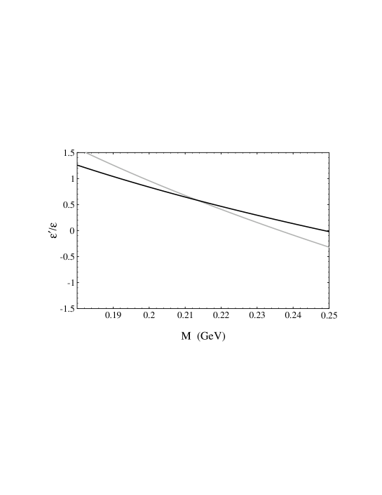
Figure 1: $\gamma_{5}$-scheme dependence of $\varepsilon^{\prime}/\varepsilon$. The black (gray) line represents the HV (NDR) result. The results are shown for $\left\langle\bar{q}q\right\rangle(0.8\ {\rm GeV})=(-200$ MeV)³, $m_{t}^{\rm pole}=180$ GeV, $\mathop{\mbox{Im}}\lambda_{t}=1.3\times 10^{-4}$ and $\Lambda_{\rm QCD}^{(4)}=350$ MeV. The stability is obtained at about $M=215$ MeV. $\varepsilon^{\prime}/\varepsilon$ is given in units of $10^{-3}$.

We find that the values at which $\gamma_{5}$-scheme independence is achieved

$$M\simeq 215-220\>\>\mbox{MeV}$$ (6.16)

are quite stable with respect to different values of the matching, the quark and the gluon condensates and $m_{t}$. Smaller values of $M$ are selected for smaller values of $\Lambda_{\rm QCD}$ (and a correspondingly higher value of $\varepsilon^{\prime}/\varepsilon$). These results are consistent with those found in II for the $\Delta I=1/2$ selection rule, where stability is achieved in the range $M=160-220$. They are also consistent with the independent estimates discussed in section 3.

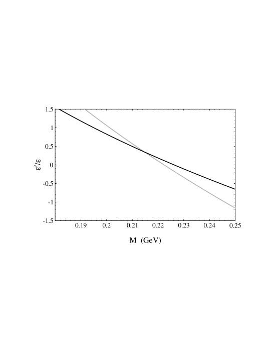
Figure 2: Same as Fig. 1 for $\left\langle\bar{q}q\right\rangle(0.8\ {\rm GeV})=(-240$ MeV)³.

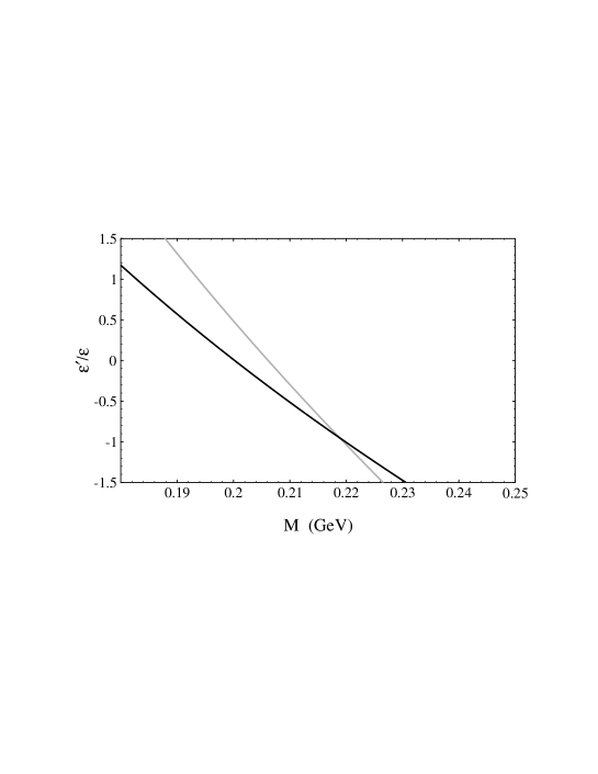
Figure 3: Same as Fig. 1 for $\left\langle\bar{q}q\right\rangle(0.8\ {\rm GeV})=(-280$ MeV)³.

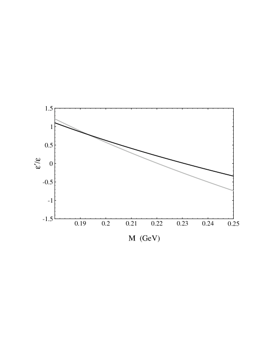
Figure 4: Same as Fig. 2 for $\Lambda_{\rm QCD}^{(4)}=250$ MeV.

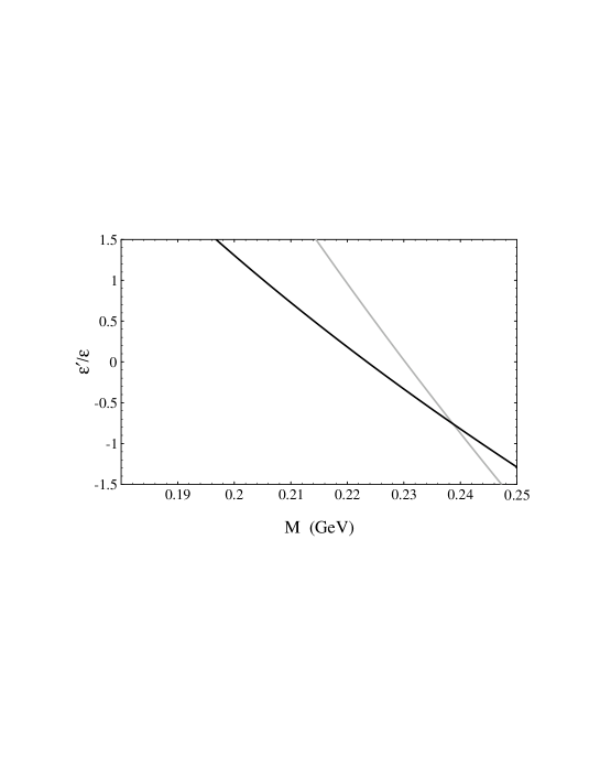
Figure 5: Same as Fig. 2 for $\Lambda_{\rm QCD}^{(4)}=450$ MeV.

As it is apparent from the figures, the final value of $\varepsilon^{\prime}/\varepsilon$ strongly depends on the value of $M$ we take. It is only through the device of requiring $\gamma_{5}$-scheme independence that we are able to reach a definite prediction. This procedure has the precious pay-off of providing us with an improved estimate that does not suffer of the uncertainty due to the $\gamma_{5}$-scheme dependence of the NLO Wilson coefficients, which may be as large as 80%.

Figs. 4 and 5 show how the intersection depends on $\Lambda_{QCD}^{(4)}$.

6.3 Anatomy of $\varepsilon^{\prime}/\varepsilon$

It is useful to consider the individual contribution to $\varepsilon^{\prime}/\varepsilon$ of each of the quark operators. We have depicted them as histograms, where the grey (black) one stands for the contribution before (after) meson-loop renormalization. Henceforth all results are given for $M=220$ MeV in the HV scheme.

It is clear from the histograms of Fig. 6, 7 and 8 that the two dominating operators are $Q_{6}$ and $Q_{8}$. Yet, since they give contributions approximately of the same size and opposite in sign, the final value turns out to be relatively small and of size comparable to that of most of the other operators. This result is at the origin the large theoretical uncertainty as well as the unexpected smallness of $\varepsilon^{\prime}/\varepsilon$.

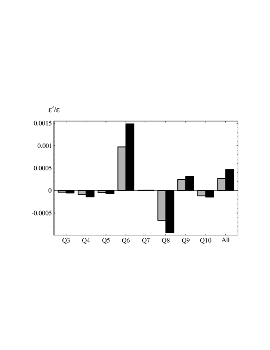
Figure 6: Histograms of the partial contributions to $\varepsilon^{\prime}/\varepsilon$ of the height relevant operators for $\left\langle\bar{q}q\right\rangle(0.8\ {\rm GeV})=(-200$ MeV)³, $m_{t}^{\rm pole}=180$ GeV, $\mathop{\mbox{Im}}\lambda_{t}=1.3\times 10^{-4}$ and $\Lambda_{\rm QCD}^{(4)}=350$ MeV. Gray (black) histograms represent the contribution of each operator without (with) meson-loop renormalization. The last two histograms correspond to the sum of all contributions.

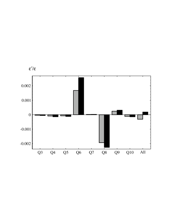
Figure 7: Same as Fig. 6 for $\left\langle\bar{q}q\right\rangle(0.8\ {\rm GeV})=(-240$ MeV)³.

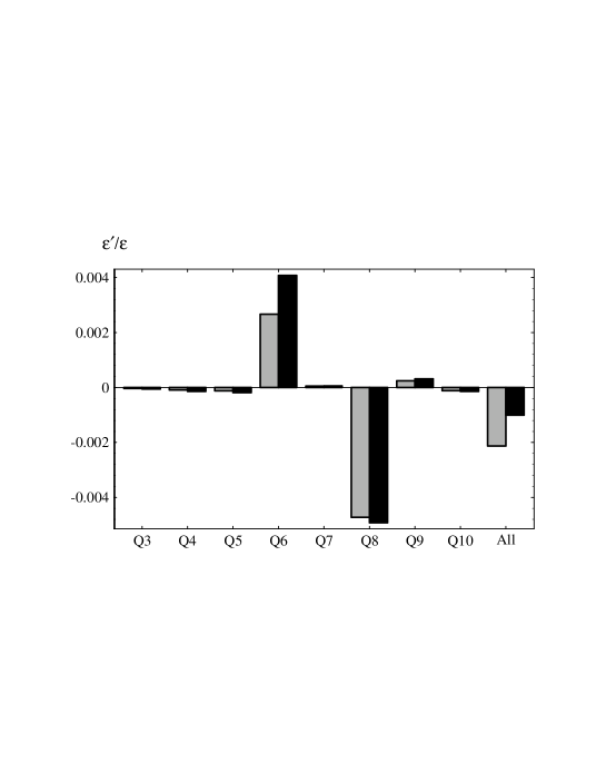
Figure 8: Same as Fig. 6 for $\left\langle\bar{q}q\right\rangle(0.8\ {\rm GeV})=(-280$ MeV)³.

The same histograms serve the purpose of showing that the meson-loop renormalizations are crucial not only in the overall size of each contribution but also in determining the sign of the final result (see Fig. 7). These corrections are here consistently included in the estimate for the first time.

The role of the operator $Q_{4}$ turns out to be marginal in our approach. In comparing this result with that of the $1/N_{c}$ framework [7] (see also the final tables in ref. [9] where we reproduce the individual $1/N_{c}$ contributions for the standard ten operators), it should be recalled that in the above analysis the $Q_{4}$ operator is written in terms of $Q_{1}$, $Q_{2}$ and $Q_{3}$ and that its values is therefore influenced by the $B_{i}$ factors assigned to the former matrix elements. In particular, while $B_{1}$ and $B_{2}$ are in ref. [7] requested to be large in order to account for the $\Delta I=1/2$ rule, $B_{3}$ is assigned the value of 1. Such a procedure produces a rather large value for the matrix element of $Q_{4}$. In our approach, we see that in fact also $B_{3}$ is large (and negative!) and that $Q_{4}$, once written in terms of the other operators, is small, as found in the direct estimate.

7 Estimating $\varepsilon^{\prime}/\varepsilon$

The preliminary work of the previous sections allows us to estimate $\varepsilon^{\prime}/\varepsilon$. The two most important sources of uncertainty are the quark condensate and the value of Im $\lambda_{t}$. Accordingly, we plot the values of $\varepsilon^{\prime}/\varepsilon$ as a function of these two quantities. Fig. 9 and 10 show our estimates, for $m_{t}$ fixed at its central value, in the first and second quadrant respectively. As it can be seen by inspecting these figures, the larger the value of the quark condensate, the swifter is the change in $\varepsilon^{\prime}/\varepsilon$.

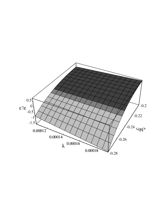
Figure 9: $\varepsilon^{\prime}/\varepsilon$ in units of $10^{-3}$ for $m_{t}^{\rm pole}=180$ GeV and $\Lambda_{QCD}^{(4)}=350$ MeV as a function of $\lambda\equiv\mathop{\mbox{Im}}\lambda_{t}$ and the quark condensate $\left\langle qq\right\rangle\equiv\left\langle\bar{q}q\right\rangle^{1/3}$ in units of GeV. Im $\lambda_{t}$ is taken in the first quadrant. Black (grey) squares represent positive (negative) values.

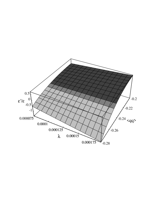
Figure 10: Same as Fig. 9 with Im $\lambda_{t}$ in quadrant II.

To have an idea of the effect of varying $m_{t}$, the third major source of uncertainty in the input parameters, we have included Fig. 11 where the top mass is varied in the given range.

Fig. 12 shows the stability of our prediction for different matching scales $\mu=0.8$ and 1 GeV (the perturbative running of $\left\langle\bar{q}q\right\rangle$ is included by taking the value of the condensate at $\mu=0.8$ GeV as the input value and than running it to $\mu=1$ GeV). The matching-scale dependence is below 20% in most of the range, becoming almost 30% only for very large values of the quark condensate.

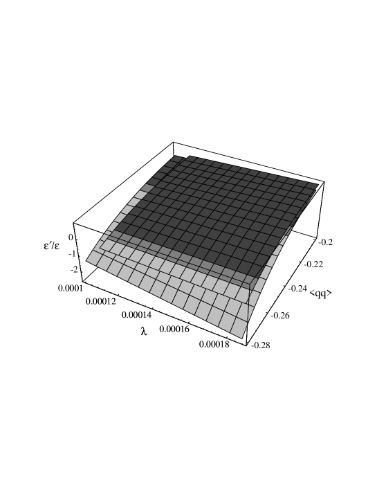
Figure 11: Same as Fig. 9 for two different values of $m_{t}$: $m_{t}^{\rm pole}=168$ GeV (upper surface) and 192 GeV (lower surface).

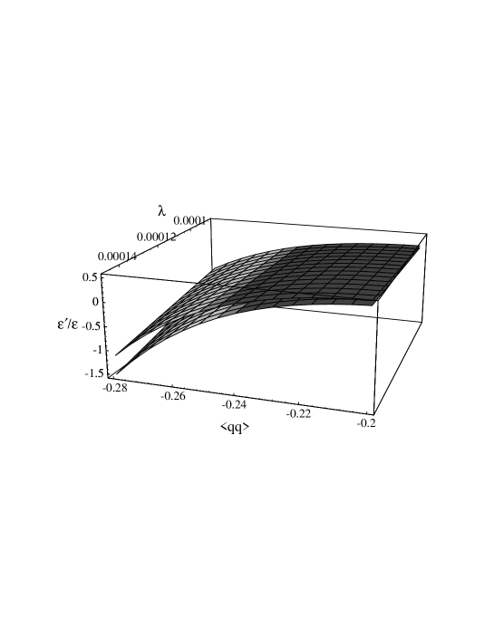
Figure 12: Same as Fig. 9 for different matching scales: $\mu=0.8$ GeV (upper surface) and 1.0 GeV (lower surface).

In order to provide the reader with a more analytical view, we have also collected in Table 4 the numerical results at the varying of all the relevant parameters.

$\Lambda_{\rm QCD}^{(4)}=250$ Mev
$\left\langle\bar{q}q\right\rangle^{(1/3)}$ (MeV)	$m_{t}^{\rm pole}$ (GeV)	quadrant I	quadrant II
	168	$3.7\div 6.5$	$2.7\div 6.3$
$-200$	180	$2.9\div 5.3$	$2.0\div 4.9$
	192	$2.1\div 3.9$	$1.4\div 4.1$
	168	$3.5\div 6.3$	$2.6\div 6.1$
$-240$	180	$1.6\div 3.0$	$1.2\div 2.8$
	192	$-0.2\div-0.4$	$-0.1\div-0.4$
	168	$-0.1\div-0.2$	$-0.1\div-0.2$
$-280$	180	$-4.1\div-7.5$	$-2.9\div-7.0$
	192	$-8.0\div-15$	$-0.5\div-16$
$\Lambda_{\rm QCD}^{(4)}=350$ Mev
$\left\langle\bar{q}q\right\rangle^{(1/3)}$ (MeV)	$m_{t}^{\rm pole}$ (GeV)	quadrant I	quadrant II
	168	$5.0\div 8.5$	$3.7\div 8.7$
$-200$	180	$3.8\div 6.9$	$2.7\div 6.6$
	192	$2.6\div 4.7$	$1.7\div 4.9$
	168	$4.3\div 7.4$	$3.2\div 7.6$
$-240$	180	$1.5\div 2.7$	$1.1\div 2.6$
	192	$-1.3\div-2.4$	$-0.9\div-2.5$
	168	$-2.3\div-4.0$	$-1.7\div-4.1$
$-280$	180	$-8.2\div-15$	$-5.7\div-14$
	192	$-14\div-26$	$-9.4\div-27$
$\Lambda_{\rm QCD}^{(4)}=450$ Mev
$\left\langle\bar{q}q\right\rangle^{(1/3)}$ (MeV)	$m_{t}^{\rm pole}$ (GeV)	quadrant I	quadrant II
	168	$8.4\div 14$	$6.2\div 14$
$-200$	180	$6.2\div 11$	$4.4\div 11$
	192	$4.0\div 7.4$	$2.7\div 6.9$
	168	$6.5\div 11$	$4.8\div 11$
$-240$	180	$1.5\div 2.7$	$1.1\div 2.6$
	192	$-3.4\div-6.2$	$-2.3\div-5.8$
	168	$-6.9\div-12$	$-5.1\div-11$
$-280$	180	$-17\div-30$	$-12\div-30$
	192	$-27\div-50$	$-18\div-47$

Table 4: Table of $\varepsilon^{\prime}/\varepsilon$ in units of $10^{-4}$. Matching scale $\mu=0.8$ GeV. The two values corresponds to, respectively, the lower and upper bounds of $\mathop{\mbox{Im}}\lambda_{t}$, which are determined by consistency with $\varepsilon$.

After twelve figures and four tables, we hope to have convinced the reader that the quantity $\varepsilon^{\prime}/\varepsilon$ is difficult to estimate with great precision. We think that only the order of magnitude can be predicted in a completely reliable manner. The reason is very simple: the final value is the result of the cancellation between two, approximately equal in size, contributions. Accordingly, even a small uncertainty will be amplified and we are unfortunately dealing with rather large ones. And yet, the shear importance of this quantity impels us to provide the best estimate we can.

By varying all parameters in the allowed ranges and, in particular, taking the quark condensate—which is the major source of uncertainty—between $(-200\ {\rm MeV})^{3}$ and $(-280\ {\rm MeV})^{3}$ we find

$$-27\times 10^{-4}\ <\varepsilon^{\prime}/\varepsilon<\ 9\times 10^{-4}\,,$$ (7.1)

where we have kept $\Lambda_{\rm QCD}^{(4)}$ fixed at its central value. A larger range,

$$-50\times 10^{-4}\ <\varepsilon^{\prime}/\varepsilon<\ 14\times 10^{-4}\,,$$ (7.2)

is obtained by varying $\Lambda_{\rm QCD}^{(4)}$ as well.

It should be stressed that the large range of negative values that we obtain is a consequence of two characteristic features of our matrix elements: i) the enhancement of the size of the electroweak matrix elements $\left\langle Q_{8,7}\right\rangle$ due to the coherent effects of the additional $O(p^{2})$ contributions so far neglected (see discussion in sect. 5) and the chiral loop corrections; ii) the linear dependence on $\left\langle\bar{q}q\right\rangle$ of the leading gluon penguin matrix elements compared to the quadratic dependence of the leading terms in the electroweak matrix elements, which makes the latter prevail for large values of the quark condensate. The effect of i) represents an enhancement of the leading electroweak matrix elements by a factor two with respect to the vacuum insertion approximation and present $1/N_{c}$ estimates (see table 3), while feature ii) is absent in the $1/N_{c}$ approach, the quark condensate dependence being always quadratic.

To provide a somewhat more restrictive estimate we may assume for the quark condensate the improved PCAC result, namely $\left\langle\bar{q}q\right\rangle=-(221\>\pm 17\ {\rm MeV})^{3}$ at our matching scale $\mu=0.8$ GeV, and thus find

$$\varepsilon^{\prime}/\varepsilon=\left\{\begin{array}[]{ll}4.5\>^{+4.1}_{-5.4}\,\times\,10^{-4}&{\rm quadrant\>I}\\ 3.9\>^{+5.0}_{-4.5}\,\times\,10^{-4}&{\rm quadrant\>II}\,.\end{array}\right.$$ (7.3)

The value of $\varepsilon^{\prime}/\varepsilon=(4\pm 5)\times 10^{-4}$ quoted in the abstract is obtained by averaging over the two quadrants in eq. (7.3).

The range (4.10) for the quark condensate, on which the above estimate is based, is not the favorite one by our analysis of the $\Delta I=1/2$ selection rule in the $\chi$QM. The upper half of the more conservative range (4.2) seems to accommodate more naturally the rule, at least for a constituent mass $M\simeq 220$ MeV—the value we find by requiring $\gamma_{5}$-scheme independence of $\varepsilon^{\prime}/\varepsilon$. For large values of the quark condensate the central values of $\varepsilon^{\prime}/\varepsilon$ shift toward the superweak regime, and the role of meson loop corrections becomes crucial.

By taking the quark condensate in the range (4.6), the QCD-SR improved PCAC result, we find

$$\varepsilon^{\prime}/\varepsilon=\left\{\begin{array}[]{ll}1.4\>^{+6.5}_{-5.5}\,\times\,10^{-4}&{\rm quadrant\>I}\\ 1.2\>^{+9.3}_{-4.0}\,\times\,10^{-4}&{\rm quadrant\>II}\,.\end{array}\right.$$ (7.4)

Actually, for such a range of $\left\langle\bar{q}q\right\rangle$, negative central values of $\varepsilon^{\prime}/\varepsilon$ in both quadrants are obtained due to the extra terms of the bosonization of the electroweak operators $Q_{7}$ and $Q_{8}$ neglected in the previous estimates. Only after the inclusion of the meson-loop renormalization $\varepsilon^{\prime}/\varepsilon$ turns to the positive central values of eq. (7.4).

Figure 13: Present status of theoretical predictions and experimental values for $\varepsilon^{\prime}/\varepsilon$ (in units of $10^{-4}$). The most recent $1/N_{c}$ [6] and lattice [5] estimates are compared to (a) our unbiased estimate (7.2), (b) our more restrictive estimate (7.3).

In Fig.13 we have summarized the present status of the theoretical predictions for $\varepsilon^{\prime}/\varepsilon$, compared to the present 1 $\sigma$ experimental results.

8 Outlook

Our phenomenological analysis, based on the simplest implementation of the $\chi$QM and chiral lagrangian methods, takes advantage of the observation that the $\Delta I=1/2$ selection rule in kaon decays is well reproduced in terms of three basic parameters (the constituent quark mass $M$ and the quark and gluon condensates) in terms of which all hadronic matrix elements of the $\Delta S=1$ lagrangian can be expressed.

We have used the best fit of the selection rule to constrain the allowed ranges of $M$, $\left\langle\bar{q}q\right\rangle$ and $\left\langle GG\right\rangle$ and we have fed them in the analysis of $\varepsilon^{\prime}/\varepsilon$.

Nonetheless, the error bars on the prediction of $\varepsilon^{\prime}/\varepsilon$ remain large. This is due to two conspiring features: 1) the destructive interference between the large hadronic matrix elements of $Q_{6}$ and $Q_{8}$ which enhances up to an order of magnitude any related uncertainty in the final prediction (this feature is general and does not depend on the specific approach); 2) the fact that large quark-condensate values are preferred in fitting the isospin zero $K^{0}\to\pi\pi$ amplitude at $O(p^{2})$ (which is a model dependent result).

Whereas little can be done concerning point 1) which makes difficult any theoretical attempt to predict $\varepsilon^{\prime}/\varepsilon$ with a precision better than a factor two, an improvement on 2) can be pursued within the present approach.

Two lines of research are in progress. On the one hand, we are extending the analysis to $O(p^{4})$ in the chiral expansion to gain better precision on the hadronic matrix elements and to determine in a self-consistent way the polinomial contributions from the chiral loops; preliminary results indicate that the $\Delta I=1/2$ rule is reproduced for smaller values of the gluon and quark condensates, thus reducing our error bar, in the direction shown by our more restrictive estimate. On the other hand, we are studying the $\Delta S=2$ sector to determine at the same order of accuracy $\hat{B}_{K}$ and the $K_{L}$–$K_{S}$ mass difference by including in the latter the interference with long-distance contributions that can be self-consistently computed in the present approach.

Whether this program is successfull may better determine how much of the long range dynamics of QCD is embedded in the present approach and increase our confidence on the predictions of unknown observables.

A Input Parameters

parameter	value
$V_{ud}$	0.9753
$V_{us}$	$0.2205\pm 0.0018$
$\sin^{2}\theta_{W}$	0.2247
$m_{Z}$	91.187 GeV
$m_{W}$	80.22 GeV
$m_{b}$	4.8 GeV
$m_{c}$	1.4 GeV
$|\varepsilon|$	$(2.266\pm 0.023)\times 10^{-3}$
$|V_{cb}|$	$0.041\pm 0.003$
$|V_{ub}/V_{cb}|$	$0.08\pm 0.02$
$m_{t}^{\rm pole}$	$180\pm 12$ GeV
$\widehat{B}_{K}$	$0.55\pm 0.25$
$f_{\pi}=f_{\pi^{+}}$	92.4 MeV
$f_{K}=f_{K^{+}}$	113 MeV
$m_{\pi}=(m_{\pi^{+}}+m_{\pi^{0}})/2$	138 MeV
$m_{K}=m_{K^{0}}$	498 MeV
$m_{\eta}$	548 MeV
$\Lambda_{\chi}$	$2\sqrt{2}\ \pi f_{\pi}$
$\Omega_{\eta+\eta^{\prime}}$	$0.25\pm 0.05$
$\Lambda_{QCD}^{(4)}$	$350\pm 100$ MeV
$\overline{m}_{u}+\overline{m}_{d}$ (1 GeV)	$12\pm 2.5$ MeV
$\overline{m}_{s}$ (1 GeV)	$178\pm 18$ MeV
$\left\langle\bar{q}q\right\rangle$	$-(200\div 280\>\mbox{MeV})^{3}$
$\langle\alpha_{s}GG/\pi\rangle$	$(376\pm 47\>\mbox{MeV})^{4}$

Table 5: Table of the numerical values of the input parameters.

References

- [1]
- [2] G.D. Barr et al. (NA31 Coll.), Phys. Lett. B 317 (1993) 233.
- [3] L.K. Gibbons et al. (E731 Coll.), Phys. Rev. Lett. 70 (1993) 1203.
- [4] A.J. Buras, M. Jamin and M.E. Lautenbacher, Nucl. Phys. B 408 (1993) 209.
- [5] M. Ciuchini, E. Franco, G. Martinelli and L. Reina, Nucl. Phys. B 415 (1994) 403; Phys. Lett. B 301 (1993) 263.
- [6] M. Ciuchini, E. Franco, G. Martinelli and L. Reina, Estimates of , in The Second DANE Physics Handbook, eds. L. Maiani et al. (Frascati, 1995); Z. Phys. C 68 (1995) 239 and references therein.
- [7] G. Buchalla, A.J. Buras and M.E. Lautenbacher, Weak Decays beyond Leading Logarithms, hep-ph/95112380, to appear in Rev. Mod. Phys..
-
[8]
J. Flynn and L. Randall, Phys. Lett. B 224 (1989) 221;
Erratum, Phys. Lett. B 235 (1990) 412;
M. Lusignoli, Nucl. Phys. B 325 (1989) 33;
G. Buchalla, A.J. Buras and M.K. Harlander, Nucl. Phys. B 337 (1990) 313. - [9] S. Bertolini, J.O. Eeg and M. Fabbrichesi, Nucl. Phys. B 449 (1995) 197.
-
[10]
K. Nishijima, Nuovo Cim. 11 (1959) 698;
F. Gursey, Nuovo Cim. 16 (1960) 230 and Ann. Phys. (NY) 12 (1961) 91;
J.A. Cronin, Phys. Rev. 161 (1967) 1483;
S. Weinberg, Physica 96A (1979) 327;
A. Manohar and H. Georgi, Nucl. Phys. B 234 (1984) 189;
A. Manohar and G. Moore, Nucl. Phys. B 243 (1984) 55. - [11] V. Antonelli, S. Bertolini, J.O. Eeg, M. Fabbrichesi and E.I. Lashin, The Weak Chiral Lagrangian as the Effective Theory of the Chiral Quark Model, preprint SISSA 43/95/EP (September 1995), hep-ph/9511255, to appear in Nuclear Physics B.
- [12] V. Antonelli, S. Bertolini, M. Fabbrichesi and E.I. Lashin, The Selection Rule, preprint SISSA 102/95/EP (October 1995), hep-ph/9511341, to appear in Nuclear Physics B.
-
[13]
M.A. Shifman, A.I. Vainsthein and V.I. Zakharov,
Nucl. Phys. B 120 (1977) 316;
F.J. Gilman and M.B. Wise, Phys. Rev. D 20 (1979) 2392;
J. Bijnens and M.B. Wise, Phys. Lett. B 137 (1984) 245;
M. Lusignoli, Nucl. Phys. B 325 (1989) 33. -
[14]
L3 Coll., Phys. Lett. B 248 (1990) 464, Phys. Lett. B 257 (1991) 469;
ALEPH Coll., Phys. Lett. B 255 (1991) 623, Phys. Lett. B 257 (1991) 479;
DELPHI Coll., Z. Phys. C 54 (1992) 55;
OPAL Coll., Z. Phys. C 55 (1992) 1;
Mark-II Coll., Phys. Rev. Lett. 64 (1990) 987;
SLD Coll., Phys. Rev. Lett. 71 (1993) 2528. - [15] L. Montanet et al., Phys. Rev. D 50 (1994) 1173 and 1995 off-year partial update for the 1996 edition (http://pdg.lbl.gov/).
- [16] J. Bijnens, Int. J. Mod. Phys. A 8 (1993) 3045.
- [17] J. Bijnens, Ch. Bruno and E. de Rafael, Nucl. Phys. B 390 (1993) 501.
- [18] S. Narison, Phys. Lett. B 197 (1987) 405.
-
[19]
E. Braaten, S. Narison and A. Pich, Nucl. Phys. B 373 (1992) 581;
S. Narison, Phys. Lett. B 361 (1995) 121;
R.A. Bertlmann et al., Z. Phys. C 39 (1988) 231. - [20] C.A. Dominguez and E. de Rafael, Ann. Phys. (NY) 174 (1987) 372.
- [21] S. Narison, hep-ph/9504333.
-
[22]
D. Daniel et al., Phys. Rev. D 46 (1992) 3130;
D. Weingarten, Nucl. Phys. B 34 (1994) 29 (Proc. Suppl.). -
[23]
M. Jamin and M. Münz, Z. Phys. C 66 (1995) 633;
C. Alton et al., Nucl. Phys. B 431 (1994) 667. - [24] J. Bijnens, J. Prades and E. de Rafael, Phys. Lett. B 348 (1995) 226.
-
[25]
W.A. Bardeen A.J. Buras and J.-M. Gérard,
Phys. Lett. B 192 (1987) 138;
W.A. Bardeen, A.J. Buras and J.-M. Gérard, Nucl. Phys. B 293 (1987) 787. -
[26]
A.J. Buras, M. Jamin and P.H. Weisz, Nucl. Phys. B 347 (1990) 491;
S. Herrlich and U. Nierste, Nucl. Phys. B 419 (1994) 292;
U. Nierste, Ph. D dissertation (Technische Universitat Munchen, 1995). -
[27]
A. Pich and E. de Rafael, Nucl. Phys. B 358 (1991) 311;
Ch. Bruno, Phys. Lett. B 320 (1994) 135;
V. Antonelli, S. Bertolini, M. Fabbrichesi and E.I. Lashin, The Parameter in the QM Including Chiral Loops, preprint SISSA 20/96/EP. - [28] A. Pich and J. Prades, Phys. Lett. B 346 (1995) 342.
- [29]