Dec. 1995 UM-TH-95-15 UCSD/PTH 95-22

The Extraction of $V_{ub}$ from Inclusive B Decays and the Resummation of End Point Logs

R. Akhoury

The Randall Laboratory of Physics

University of Michigan

Ann Arbor MI 48109

I.Z. Rothstein

Dept. of Physics

UCSD

La Jolla Ca. 92093

Abstract

In this paper we discuss the theoretical difficulties in extracting $V_{ub}$ using the data from inclusive B decays. Specifically, we address the issue of the end point singularities. We perform the resummation of both the leading and next to leading end point logs and include the leading corrections to the hard scattering amplitude. We find that the resummation is a $20\%-50\%$ effect in the end point region where the resummation is valid. Furthermore, the resummed sub-leading logs dominate the resummed double logs. The consequences of this result for a model independent extraction of the mixing angle $V_{ub}$ are explored.

1 Introduction

Measurements in the bottom quark sector have reached the point that our knowledge of many observables is now bounded by the theoretical uncertainties [1]. Fortunately, theoretical advances in calculating both exclusive as well as inclusive rates now allow the extraction of the CKM parameters without recourse to the models which have soiled the extraction processes to data. The present values of $V_{ub}$ have a model dependence which introduce an uncertainty of a factor of 2[1], which is several times larger than the experimental uncertainties. With QCD based calculations, we can now hope to extract both $V_{bc}$ and $V_{ub}$ with errors on the order of tens of percents. In this work, we concentrate on the extraction of $V_{ub}$ from the measurement of the electron spectrum in semi-leptonic inclusive B meson decays.

The extraction of $V_{ub}$ from inclusive semi-leptonic B decays is hindered by the fact that the background from charmed decays is overwhelming for most of the range of the lepton energy. Thus, we are forced to make a cut on the lepton energy, vetoing all events, or some large fraction thereof, with lepton energy less than the $b\rightarrow c$ end point energy. Given the proximity of the two relevant end points, this obviously hinders the statistics. However, even with a large data sample, the accuracy of the extraction will be limited by the errors induced from the approximations used in calculating the theoretical prediction in the end point region. This region of the Dalitz plot is especially nettlesome for theory, because the perturbative, as well as the non-perturbative corrections become large when the lepton energy is near its endpoint value.

It has been shown that it is possible to calculate the decay spectrum of inclusive heavy meson decay in a systematic expansion in $\epsilon=\frac{\Lambda_{QCD}}{m_{b}}$ and $\alpha_{s}$ using an operator product expansion within the confines of heavy quark effective field theory[2]. It is possible to Euclideanize the calculation of the rate for most of the region of the Dalitz plot with only minimal assumptions about local duality. However, in the end point region, the expansion in $\epsilon$, as well as the expansion in $\alpha_{s}$, begin to breakdown (The endpoint region poses problems for local duality as well. We shall discuss this in more detail later).

The aim of this paper is to determine the size of the errors induced from the theoretical uncertainties in extraction of $V_{ub}$. A large piece of this work consists of implementing the resummation of the leading and sub-leading endpoint logs which cause the breakdown of the expansion in $\alpha_{s}$, as first discussed on general grounds in [3], and the inclusion of the $\alpha_{s}$ corrections to the hard scattering amplitude. However, to determine the consistency of our calculation, we must also address the issue of the non-perturbative corrections. These issues have been previously looked at in refs [4] and [6]. In [4] the need for resummation was addressed on general grounds. However, the calculational methods used here are not compatible with the arguments given in [4], and thus we must recapitulate these arguments within the confines of our methods.

In the second section of this paper, we discuss the question of the need to resum the perturbative as well as non-perturbative series. The next three sections are dedicated to the resummation of the leading and next to leading infrared logs and the inclusion of the one loop corrections to the hard scattering amplitude (read one loop matching). In the fifth section we give our numerical results while the last section draws conclusions regarding what errors we can expect in the extraction process.

2 Is Resummation Necessary?

As mentioned above, the theoretical calculation of the lepton spectrum in inclusive decays breaks down near the endpoint. Both the non-perturbative as well as perturbative corrections become large in this region. Here we investigate the need to perform resummations in either or both of these expansions. The one loop decay spectrum including the leading non-perturbative corrections is given by [10]

$$\frac{1}{\Gamma_{0}}\frac{d\Gamma}{dx} = \theta(1-x)\left[x^{2}(3-2x)(1-\frac{2\alpha_{s}}{3\pi})I(x)+2(3-x)x^{2}E_{b}-\frac{2}{3}x^{2}(9+2x)K_{b}-\frac{2}{3}x^{2}(15+2x)G_{b}\right]$$ (1)

$$+ \left[E_{b}-\frac{2}{3}K_{b}+\frac{8}{3}G_{b}\right]\delta(1-x)+\frac{1}{3}K_{b}\delta^{\prime}(1-x).$$

Where

$$I(x)=\log^{2}(1-x)+\frac{31}{6}\log(1-x)+\pi^{2}+\frac{5}{4}~{}~{}{\rm{and}}~{}~{}x=\frac{2E_{e}}{m_{b}},$$ (2)

$$\Gamma_{0}=\mid V_{ub}\mid^{2}\frac{G_{F}^{2}m_{b}^{5}}{96\pi^{3}}.$$ (3)

$E_{b},~{}G_{b}$ and $K_{b}$ are hadronic matrix elements of order $\epsilon^{2}$ and are given by

$$E_{b} = G_{b}+K_{b},$$

$$K_{b} = \langle B(v)\mid\bar{b}_{v}\frac{D^{2}}{2m_{b}^{2}}\mid B(v)\rangle,$$

$$G_{B} = \langle B(v)\mid\bar{b}_{v}g\frac{\sigma_{\alpha\beta}G^{\alpha\beta}}{4m_{b}^{2}}b_{v}\mid B(v)\rangle,$$ (4)

$b_{v}$ is the velocity dependent bottom quark field as defined in heavy quark effective field theory. From the above expressions we see that the breakdown of the expansions, in $\alpha_{s}$ and $\epsilon=\frac{\Lambda_{QCD}}{m_{b}}$, manifest themselves in the large logs and the derivative of delta functions, respectively.

2.1 The non-perturbative expansion

As one would expect for heavy meson decay, the leading order term in $\epsilon$ reproduces the parton model result. All corrections due to the fact that the b quark is in a bound state are down by $\epsilon^{2}$ [2]. However, near the end point of the electron spectrum we begin to probe the non-perturbative physics. The general form of the expansion in $\epsilon=\frac{\lambda}{m_{b}}$, to leading order in $\alpha_{s}$, is given as follows

$${1\over{\Gamma_{0}}}{d\Gamma\over{dx}} = \theta(1-x)\left(\epsilon^{0}+\epsilon^{2}+\cdot\cdot\cdot\right)+\delta(1-x)\left(0\epsilon+\epsilon^{2}+\epsilon^{3}+\cdot\cdot\cdot\right)$$ (5)

$$+ \cdot\cdot\cdot+\delta^{(n)}(1-x)\left(\epsilon^{n+1}+\epsilon^{n+2}+\cdot\cdot\cdot\right)+\cdot\cdot\cdot$$ (6)

The end point singularities are there because the true end point is determined by the mesonic mass and not the partonic mass, as enforced by the theta function in the leading order term. The difference between these end points will be on the order of a few hundred MeV. To make sense of this expansion we must smear the decay amplitude with some smooth function of $x$. Normally, this would not pose a problem, however, given that the distance between the $b\rightarrow c$ and $b\rightarrow u$ end points is approximately $330~{}MeV$, we are forced to integrate over a weighting function which has support in a relatively small region. On the other hand, if the weighting function is too narrow, then the expansion in $\epsilon$ will not be well behaved.

Thus we must find a smearing function that minimizes the errors due to ${\Lambda_{QCD}\over{m_{b}}}$ corrections which does not overlap with the energy region where we expect many $b\rightarrow c$ events. The question then becomes how many $b\rightarrow c$ transitions can we allow without introducing large errors due to our ignorance of the $b\rightarrow c$ end point spectrum (the theory breaks down in the $b\rightarrow c$ end point region as well though there are important differences between this case and the $b\rightarrow u$ transitions)?

The issue of smearing was addressed by Falk et. al.[4] who used Gaussian smearing functions to gain quantitative insight into the need for smearing. They found that without any resummation, the smearing function should have a width which is greater than $\epsilon$, but that after resumming the leading singularities, we need smear only over a region of width $\epsilon$. Here we will smear by taking moments of the electron energy spectrum (we work with the moments of the spectrum because it greatly facilitates the resummation of the perturbative corrections). Thus, we must address the question of what range of values of $N$ will lead to a sensible expansion which is also not overly contaminated by $b\rightarrow c$ transitions? This will obviously depend on the ratio of $V_{ub}$ to $V_{bc}$. To get a handle on the numerics, let us for the moment assume that we wish that the number of $b\rightarrow u$ transitions be at least equal to the number of $b\rightarrow c$ transitions in our sample. In figure 1., we plot $\frac{V_{ub}^{2}}{V_{bc}^{2}}(N)$, which is the ratio of mixing angles for which the $N$th moments of the leading order rates for $b\rightarrow c$ and $b\rightarrow u$ transitions will be equal, and is given by

$$\frac{V_{ub}^{2}}{V_{bc}^{2}}(N)=\frac{\displaystyle\int^{x_{m}}_{0}x^{2}{(x_{m}-x)^{2}\over{(1-x)^{3}}}[6-3x_{m}+(x_{m}-6)x+2x^{2}]x^{N}dx}{\displaystyle\int^{1}_{0}x^{2}(3-2x)x^{N}}.$$ (7)

$x_{m}$ is $\frac{2E_{max}}{m_{b}}$ for the $B\rightarrow D$ transitions and takes the value $x_{m}\approx.9$. Given the bounds [5]

$$.002<\frac{\mid V_{ub}\mid^{2}}{\mid V_{bc}\mid^{2}}<.024,$$ (8)

we see that an understanding of the spectrum for moments around $N\simeq 20$ is necessitated if we wish to keep the $b\rightarrow c$ contamination under control (Of course we do not suggest that these moments can be measured given the finite resolution of the experiment. We will discuss this situation later in the paper).

Figure 1: The ratio of $\frac{V_{ub}^{2}}{V_{bc}^{2}}$ for which the Nth moments of the leading order spectra are equal.

We now consider the issue of determining the maximum value of $N$ for which the expansion makes sense. Let us first consider the expansion in $\epsilon$. The moments of the leading singularities of eq.(5) will behave as

$$M_{N}\approx C_{n}\frac{N!\epsilon^{n+1}}{(N-n)!}.$$ (9)

As a possible criterion on the size of $N$, we may impose that there be no growth with n. That is

$$\frac{N!\epsilon^{n+1}\left(ln\epsilon+\Psi(N-n+1)\right)}{(N-n)!}<0.$$ (10)

$\epsilon$ represents the value of some matrix element in the heavy quark effective theory. It is assumed that the value of $\epsilon$ should be on the order of a few hundred $MeV/m_{b}$, but in theory it could vary by a factor of order one from term to term. To get a handle on the sizes of $\epsilon$, we may consider the leading $\epsilon$, which is given by

$$\epsilon_{1}=\langle B\mid\bar{b}_{v}\frac{(iD)^{2}}{2}b_{v}\mid B\rangle\frac{1}{m_{b}^{2}}.$$ (11)

Quark model calculations suggest that $\epsilon_{1}^{2}$ is on the order of .01[7]. Thus, naively, it seems that to keep the expansion in $\epsilon$ under control, we must keep $N\leq 10$. This estimate is perhaps too crude for our purposes given that we know nothing of the growth of the coefficients $C_{n}$ nor of the range of possible values of $\epsilon_{N}$, it does suggest that some sort of resummation may be necessary.

Neubert[7] pointed out that it is possible to resum the leading singularities, much as in the case of deep inelastic scattering, into a non-perturbative shape function

$$\tilde{f}(k_{+})=\langle B\mid\delta(k_{+}-iD_{+})\mid B\rangle.$$ (12)

This function gives the probability to find the $b$ quark within the hadron with residual light cone momentum $k_{+}$. Thus, this function is roughly determined by the kinetic energy of the b quark inside the meson. This structure function will be centered around zero and have some characteristic width $\delta$. $\delta$ will determine the maximum size of $N$ for which the expansion without resummation makes sense. To get a well behaved expansion we choose $N$ such that $x^{N}$ gives order one support to the structure function throughout its width. The value of $\delta$ is unknown at this time, and various authors have given different estimates for its value. We can assume that this width should be on the order of $(m_{B}-m_{b})/2$ which is around 300 $MeV$. We shall choose, what we believe to be the conservative value of 500 $MeV$ for $\delta$. Since the structure function is the sum of derivatives of delta functions, we conclude that we should smear over the width of the function if we do not wish to incur large errors. Let us assume, for the sake of numerics, that $x^{N}$ should not fall below the value .1, within 500 $MeV$ of the end point. Then we find that $N$ must be $\leq 20$. Thus, we expect the non-perturbative effects could be quite large for the range of $N$ that we consider here. Of course when $N$ becomes very large, $N>100$, it is necessary to go beyond leading twist since the soft gluon exchange in the t channel begins to dominate, not to mention the failure of the OPE due to its asymptotic nature [8].

We see that for our purposes we should include the non-perturbative structure function in our calculation. The fact that the knowledge of this non-perturbative function is needed to extract $V_{ub}$ should not bother us too much however, given that it is universal. That is to say we can remove it from our final result by taking the appropriate ratio [11]. Or it can be measured on the lattice, much in the same way that the moments of the proton structure functions are now being measured. Using the ACCMM model [9] Blok and Mannel [6] concluded that a resummation of the non-perturbative corrections is unnecessary. If the width of the structure function is smaller than the conservative number chosen here, then this could very well be true. This would be a welcomed simplification of the extraction process, since we would no longer need to rely on the extraction of non-perturbative parameters from other processes to measure the mixing angle $V_{ub}$.

2.2 The perturbative expansion

Let us now address the issue of the perturbative corrections. The corrections in $\alpha_{s}$ grow large near the electron energy end point, and, precisely at the end point, there are logarithmic infrared divergences. These divergences are due to the fact that near the end point gluon radiation is inhibited, and as a result, the usual cancelation of the infrared divergences between real and virtual gluon emission is nullified. Of course, the rate is not divergent, and we expect that a resummation procedure will have the effect of reducing the rate for the exclusive process.

Near the end point large logs form a series of the form

$${d\Gamma\over{dx}} = C_{11}\alpha Log^{2}[1-x]+C_{12}\alpha Log[1-x]+C_{13}\alpha$$

$$+ C_{21}\alpha^{2}Log^{4}[1-x]+C_{22}\alpha^{2}Log^{3}[1-x]+\cdots$$

$$+ C_{31}\alpha^{3}Log[1-x]^{6}+C_{32}\alpha^{3}Log^{5}[1-x]+\cdots$$

$$+ ~{}~{}~{}~{}~{}~{}~{}~{}~{}~{}~{}.~{}~{}~{}~{}~{}~{}~{}~{}~{}~{}~{}+~{}~{}~{}~{}~{}~{}~{}~{}~{}.~{}~{}~{}~{}~{}~{}~{}~{}~{}~{}~{}~{}+\cdots$$

$$+ ~{}~{}~{}~{}~{}~{}~{}~{}~{}~{}~{}.~{}~{}~{}~{}~{}~{}~{}~{}~{}~{}~{}+~{}~{}~{}~{}~{}~{}~{}~{}~{}.~{}~{}~{}~{}~{}~{}~{}~{}~{}~{}~{}~{}+\cdots$$

Which in terms of a moment expansion gives (for large $N$)

$$\int^{1}_{0}dxx^{N}{d\Gamma\over{dx}}= \frac{1}{N}\left(\tilde{C}_{11}\alpha Log^{2}N+\tilde{C}_{12}\alpha LogN+\tilde{C}_{13}\alpha\right.$$

$$+ \tilde{C}_{21}\alpha^{2}Log^{4}N+\tilde{C}_{22}\alpha^{2}Log^{3}N+\cdots$$

$$+ \left.\tilde{C}_{31}\alpha^{3}LogN^{6}+\tilde{C}_{32}\alpha^{3}Log^{5}N+\cdots\right).$$

Given this expansion, we may ask what errors we expect to incur by truncating the expansion at order $\alpha_{s}$? For $N$ near 20, we see that

$${\alpha_{s}\over{\pi}}Log^{2}N\simeq.6,$$ (14)

so we might expect that truncating at leading order would not be such a good idea. We must also note that in (1) the sub-leading log actually dominates the leading double log due to the large coefficient $\frac{31}{6}$. The resummation of the double logs is simple and leads the the exponentiation of the double logs. Figure 2 shows the difference between the one loop result and the result with only the double logs resummed. We see that the difference is very small, on the order of five percent. Thus, one might come to the conclusion that no resummation of the perturbative series is necessary. However, given that the coefficients of the single logs as well as the $\pi^{2}$, which are just as large as the double logs for the range of $N$ we are considering here, are unknown at higher orders, we can only determine the errors induced by a truncation of the series after we have performed the resummation.

Figure 2: The difference between the moments given by the leading $\alpha_{s}$ correction and the moments of the rate with only the double logs resummed.

Resumming the leading double logs in itself does not increase the range in $N$ over which perturbation theory is valid. Even after this resummation is performed the criteria for a convergent expansion is still $\frac{\alpha_{s}}{\pi}Log^{2}N<1$ unless we know that the subleading logs exponentiate as well. However, one can show on very general grounds [12] that all the end point logs exponentiate as a consequence of the fact that these logs are really just UV logs in the effective field theory[24, 17]. Thus it is always possible to write down a differential equation for the rate based on its factorization scale independence. As such, the general form of the decay amplitude will be given by

$$Log\left[\int^{1}_{0}\frac{d\Gamma}{dx}x^{N}\right]=C(\alpha_{s})+\sum_{n=1}^{\infty}\alpha^{n}_{s}\sum^{2n}_{m=1}G_{nm}Log^{m}N.$$ (15)

Once we have this information, the question of the region of convergence becomes, do the lower order terms in question contribute numbers of order 1 in the exponent? We may continue to increase $N$ until we find that the subleading terms in the exponent contribute on the order 1. Thus in general resumming the leading logs does indeed allow us to take $N$ into the range where $\frac{\alpha_{s}}{\pi}Log^{2}N\simeq 1$. Here we will go further, as was done in [3], and sum the next to leading logs as well, allowing $\frac{\alpha_{s}}{\pi}LogN\leq 1$. This will allow us to determine the convergence of the expansion. Furthermore, we extend the analysis of [3] to include the one loop matching corrections thus completing the calculation at order $\alpha_{s}$.

We wish to note that Blok and Mannel [6] analyzed the effects of the large logs to the end point spectrum and concluded that no resummations were necessary. These authors propose to take the lower bound on the moment integral to be the charmed quark endpoint $x_{c}$. Doing this allows one to stay away from larger values of $N$ (the authors choose $N<10$). Cutting off the integral introduces errors that have the doubly logarithmic $x_{c}$ dependence $ln^{2}(1-x_{c})$. To reduce these errors, it is necessary to go to higher values of $N$. These authors claim that for $N<10$, the errors induced by cutting off the integral are small, on the order of a few percent. However, we believe that these authors have underestimated their errors because they normalized their errors by the total width and not the moments themselves. Furthermore, and perhaps most importantly, the authors did not consider the possibility that the sub-leading logs could dominate the leading logs in the resummation, which as we shall see, is indeed the case.

Finally, it should be pointed out that aside from being bounded by the size of the logs, $N$ is bounded on purely logical grounds. The whole perturbative QCD framework loses meaning when the time scale for gluon emission becomes on the order of the hadronization time scale. This restriction bounds the minimum virtuality of the gluon, which we expect to be on the order of $\frac{m_{b}}{N}$(we will show this to be true when we perform the resummation). Thus, performing resummations can only take one so far no matter how powerful one is. However, for top quark decays it is possible to get extremely close to the end point due to the large top quark mass. In this case it is clear that the resummation of the next to leading logs will become essential. Thus, the extraction of $V_{td}$ from inclusive top quark decays will have much smaller theoretical errors than in the b decay case. We shall discuss the issue of the breakdown of perturbation theory in greater detail after we perform the resummation.

3 Factorization

The large logs appearing in the perturbative expansion arise from the fact that at the edge of phase space gluon emission is suppressed. The problem of summing these large corrections has been treated previously for various applications, such as deep inelastic scattering and Drell-Yan processes[12, 13], just to mention a few. The case of inclusive heavy quark decay has been treated previously in [3]. An important ingredient of the resummation procedure is the proof of factorization. As applied to the present processes, this procedure separates the particular differential rate under consideration into sub-processes with disparate scales.

In the case of inclusive semi-leptonic heavy quark decays, the relevant scales are $m_{b}$ and $m_{b}(1-x)$, with $x={2E_{e}\over{m_{b}}}$ in the rest frame of the b-quark. To understand how to best factorize the differential rate in the limit $x\rightarrow 1$, we need to know the momentum configurations which give leading contributions in that limit. With this in mind, let us consider the inclusive decay of the b-quark into an electron and neutrino of momenta $p_{e}$ and $p_{\nu}$ respectively, and a hadronic jet of momenta $p_{h}$. First we note that the kinematic analysis is simplified with the following choice of variables in the rest frame of the b quark[27]

$$x={2E_{e}\over{m_{b}}}~{}~{}~{}y_{0}={2(E_{e}+E_{\nu})\over{m_{b}}}~{}~{}~{}y={(p_{e}+p_{\nu})^{2}\over{m_{b}^{2}}}.$$ (16)

The kinematic ranges for these variables are

$$0\leq x\leq 1;~{}~{}0\leq y\leq x;~{}~{}({y/x}+x)\leq y_{0}\leq(y+1).$$ (17)

Furthermore, define the variable

$$\eta=\left({1-y\over{2-y_{0}}}\right)~{}~{}\rm{where}~{}~{}x\leq\eta\leq 1.$$ (18)

This variable plays an analogous role to the Bjorken scaling variable in deep inelastic scattering phenomena. The invariant mass of the final state hadronic jet, and its energy are given by

$$p_{h}^{2}=m_{b}^{2}(1-\eta)(2-y_{0}),~{}~{}~{}p_{h}^{0}=\frac{m_{b}}{2}(2-y_{0}).$$ (19)

We should note that in determining the boundary values of the various variables we refer to the b-quark mass and not to that of the meson. This is justified within the perturbative framework we are working in at the moment. However, once we include the effects of the non-perturbative structure function, the phase space limits will take on their physical values.

Let us now investigate the dominant momentum configurations near $x\rightarrow 1$. First, we observe that the invariant mass of the hadronic jet $+$ neutrino system is given by $(p_{b}-p_{e}-p_{\nu})^{2}={m_{b}^{2}}(1-x)$ which vanishes at the end point. The phase space configuration where the neutrino is soft is suppressed and hence, when the value of $x$ approaches one, the electron and the hadronic jet-neutrino system move back to back in the rest frame of the b-quark. Furthermore, the invariant mass of the hadronic jet vanishes independently of the neutrino energy. This is readily verified using the phase space boundaries. The energy of the jet is large except near the point $x\rightarrow y\rightarrow 1$. In this region of the Dalitz plot factorization breaks down, and the techniques used here fail. However, this problematic region is irrelevant as a consequence of the fact that the rate to produce soft massless fermions are suppressed at the tree level. Thus, the following picture emerges at $x\sim 1$. The b-quark decays into an electron moving back to back with the neutrino and a light-like hadronic jet. We choose the electron to be moving in the $+$ (light cone) direction, and the jet moves in the $-$ (light cone) direction in the rest frame of the b-quark. The constituents of the jet may interact via soft gluon radiation with each other and with the b-quark, but hard gluon exchange is disallowed.

This simple picture is related by the Coleman-Norton theorem [14, 16] to the type of Feynman diagrams that are infrared sensitive. According to this theorem, if we construct a “reduced” diagram by contracting all off shell lines to a point, then at the infrared singular point, such a diagram describes a physically realizable process. Thus at $x\sim 1$ the type of diagrams that give large logs are precisely those described above and shown in figure 3.

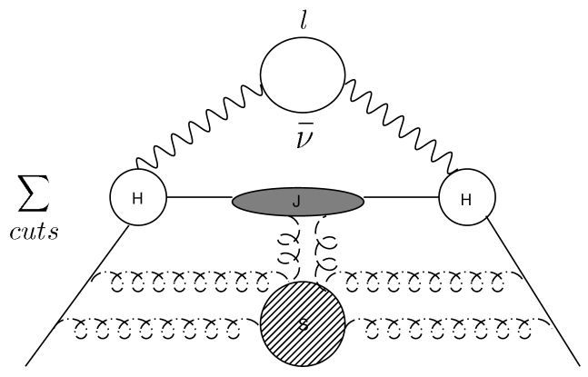
Figure 3: Reduced diagram for B decays.

In the figure, S denotes a soft blob which interacts with the jet and the b-quark via soft lines. J denotes the hadronic jet and H the hard scattering amplitude. The typical momenta flowing through the hard sub-process are $O(m_{b})$. H does not contain any large end point logs and has a well defined perturbative expansion in $\alpha_{s}(m_{b})$. All the lines which constitute H are off-shell and have been shrunken to a point. The soft function S contains typical soft momentum $k$ , with $k^{+}\sim k^{-}\sim k_{\perp}\sim O(m_{b}(1-x))$. Thus, by “soft” we mean soft compared to $m_{b}$, but still larger than $\Lambda_{QCD}$. The jet subprocess has typical momenta $p$ such that $p^{-}\gg p^{+},p_{\perp}^{2}$ with $p^{+},p_{\perp}^{2}\sim O(m_{b}(1-x))$ and $p^{-}\sim O(m_{b})$. In order to delineate between momentum regimes, a factorization scale $\mu$ is introduced. The fact that the process is $\mu$ independent will be utilized to sum the large end point logs which are contained in the soft and jet functions. The reduced digram for the inclusive radiative decay $b\rightarrow X_{s}\gamma$ is exactly the same as above if we ignore the strange quark mass.

An important consequence of the factorization is the fact that the soft function, $S$, is universal. That is, it is independent of the final states as long as factorization holds. Thus the soft function in the semi-leptonic decay will be the same soft function as in the radiative decay. This universality will allow us to remove our ignorance of any nonperturbative physics due to bound state dynamics by taking the appropriate ratio. Thus, throughout this paper we will treat both the semi-leptonic as well as the radiative decays in turn.

We conclude this discussion with a few comments. First, we should point out the differences between factorization in the process considered here and in deep inelastic scattering for large values of the Bjorken scaling variable[13]. A crucial difference arises from the fact that the initial quark is massive, and hence, the semi-inclusive decays of the a heavy quark is infrared finite to all orders in perturbation theory because there are no collinear divergences arising from initial state radiation. This fact has the important consequence that the differential decay rate will be independent of $\mu$. Whereas $\mu$ independence in deep inelastic scattering is only achieved after an appropriate subtraction is made with another process, such as Drell-Yan, which has the same collinear divergence structure as the deep inelastic scattering process. Next we note that, in general, the separation of diagrams into soft and jet subprocesses is not unique, and some prescription must be adopted. For a discussion of this issue see [22, 12]. In our case, we will determine the proper separation from the requirement of the $\mu$ independence of the decay rate from the condition that the hard scattering amplitude does not contain any large end point logs, and that the purely collinear divergences in the jet must satisfy an Altarelli-Parisi like evolution equation. We will return to this point in the next section. The factorization can be made more manifest by going to the light like axial gauge with the gauge fixing vector pointing in the jet direction. In this gauge, the soft lines decouple from the jet on a diagram by diagram basis.

In terms of the variables introduced earlier, the triply differential factorized decay amplitude may be written as

$${1\over{\Gamma^{0}}}{d^{3}\Gamma\over{dxdydy_{0}}}={6m_{b}(x-y)(y_{0}-x)}\int^{k^{+}_{max}}_{k^{-}_{min}}dk_{+}f(k^{+},\mu^{2})J(p_{h}^{-}(p_{h}^{+}-k^{+}),\mu^{2})H(m_{b},\mu^{2}),$$ (20)

$$\Gamma^{0}={G_{F}^{2}\over{96\pi^{3}}}\mid V_{ub}\mid^{2}m_{b}^{5}.$$ (21)

This form will hold up to errors on the order of $O(1-x)$.

We have chosen the electron to be traveling in the $+$ direction with momenta $k=m_{b}(x,0,0_{\perp})$, and

$$k^{+}_{max}=m_{b}(1-\eta),~{}~{}k^{+}_{min}=-(M_{B}-m_{b}).$$ (22)

Here $f(k^{+})$ is the probability for the $b$ quark to have light cone residual momentum $k^{+}$, and thus contains not only the information in the soft function $S$ but also the non-perturbative information regarding the nature of the bound state. If we ignore perturbative “soft” gluon radiation, then this function coincides with $\tilde{f}(k_{+})$ defined in the previous section. Notice that $k_{+}^{min}$ is negative. This is important non-perturbatively and represents the leakedge past the partonic end point due to the soft gluon getting energy and momentum from the light degrees of freedom inside the B meson. Loosely speaking it is due to the Fermi motion of the b- quark inside the meson.

Less formally, we may write the derivative of the decay amplitude as [3]

$${-1\over{\Gamma_{0}}}{d\over{dx}}\left({d\Gamma\over{dx}}\right)=\int^{2}_{1}dy_{0}6(2-y_{0})^{2}(y_{0}-1)G(x),$$ (23)

$$G(x)=\int_{x}^{M_{B}/m_{b}}dzf(z,m_{b}/\mu)J(m_{b}^{2}(2-y_{0})(z-x),\mu^{2})H(m_{b}(2-y_{0})/\mu).$$ (24)

In this equation we have changed variables from $k^{+}$ to the residual light cone momentum fraction $z=(1-{k^{+}\over{m_{b}}})$, and absorbed a factor of $m_{b}^{2}$ into the jet factor.

By taking the moments of this expression with respect to $x$ we see that we are able to treat the hard, soft and jet functions separately. We are led to the following form for the moments of the semi-leptonic rate

$$M_{N}^{sl} \equiv \frac{1}{\Gamma_{0}}\int^{M_{B}/m_{b}}_{0}x^{N-1}{d\over{dx}}\left({d\Gamma\over{dx}}\right)dx=$$ (27)

$$\int^{2}_{1}dy_{0}6(2-y_{0})(y_{0}-1)f_{N}J_{N}(m_{b}^{2}(2-y_{0}),\mu^{2})H(m_{b}(2-y_{0}),\mu),$$

$$f_{N}=\int^{M_{B}/m_{b}}_{0}z^{N}dzf(z),$$

$$J_{N}(2-y_{0})=\int^{1}_{0}\lambda^{N}J(m_{b}^{2}(2-y_{0})(1-{\lambda},\mu^{2}))d\lambda.$$

In writing the last few equations we have dropped all terms of order $O(1-x)$ or equivalently taken the large $N$ limit. The left hand side of Eq(27) defines the moments of the semi-leptonic decay electron distribution, $M_{N}^{sl}$.

The moments of the soft function $f_{N}$ may be decomposed into a product of moments of a perturbatively calculable $\sigma_{N}$ and the non-perturbative structure function $S_{N}$, which corresponds to the moments of $\tilde{f}$ discussed in the previous section. We may write

$$\tilde{f}(z)=\int^{M_{B}/m_{b}}_{z}{dy\over{y}}S(y)\sigma({z\over{y}}),$$ (28)

and thus, taking moments,

$$f_{N}=\sigma_{N}S_{N}.$$ (29)

An analogous situation exists for the decay $B\rightarrow X_{s}\gamma$. We define $x={2E_{\gamma}\over{m_{b}}}$ in the rest frame of the b-quark, and take the photon to be moving in the $+$ direction, and, as in the semi-leptonic decay, at $x\sim 1$ the hadronic jet is moving in the $-$ direction. Furthermore, the invariant mass of the hadronic jet and its energy are

$$p_{h}^{2}=m_{b}^{2}(1-x),~{}~{}~{}p_{h}^{0}=m_{b}(1-x/2).$$ (30)

Thus the s-quark is very energetic and since the invariant mass of the jet vanishes as $x\sim 1$, the s-quark decays into quanta which are collinear once we ignore effects on the order of $\frac{m_{s}^{2}}{m_{b}^{2}}$. Clearly the factorization picture discussed earlier for the semi-leptonic decay holds here as well and the reduced diagram is the same as in fig(3).

As before we may take the moments of the differential rate

$$M_{N}^{\gamma}\equiv{1\over{\Gamma_{\gamma}}}\int^{M_{B}/m_{b}}_{0}dxx^{N-1}{d\Gamma\over dx}=S_{N}\sigma_{N}J_{N}.$$ (31)

where[31],

$$\Gamma_{\gamma}={{\alpha G_{F}^{2}}\over{32\pi^{4}}}m_{b}^{5}\mid V_{tb}V_{ts}^{*}\mid^{2}C_{7}^{2}(m_{b}).$$ (32)

and

$$J_{N}=\int_{0}^{1}dyy^{N-1}J(m_{b}^{2}(1-y),\mu^{2}).$$ (33)

$\sigma_{N}$ and $S_{N}$ are the same functions defined in (28) and $C_{7}$ is the Wilson coefficient of $O_{7}$ as defined in [31]. For the radiative decay, the $ln(1-x)/(1-x)_{+}$ distribution in the amplitude will correspond to $ln^{2}(N)$ in the moment. Whereas, in the semi-leptonic decay, taking the derivative of the amplitude will generate plus distributions which will then generate $LogN$ and $Log^{2}N$ after taking the moments. Thus, we have reduced the problem of the resummation of the large logs in the amplitude to resumming the logs in $J_{N}$ and $\sigma_{N}$ separately. This greatly simplifies the calculation as will be seen below.

4 Resummation

The resummation of the infrared logs is analogous to summing ultra violet logs. One takes advantage of the $\mu$ independence of the amplitude. In the case of infra-red logs, $\mu$ is the factorization scale, or equivalently the renormalization scale within the appropriate effective field theory, which for this case would the field theory of Wilson lines [17].

We first outline the derivation of a representation of the soft function $\sigma_{N}$ near $x=1$ following the techniques developed in reference [13]. We will work in the eikonal approximation where soft momenta are ignored wherever possible. At the one loop level, the real gluon emission contribution factorizes and the quantity multiplying the tree level rate is

$$F_{eik}^{real}(x)=g^{2}C_{F}\int{d^{3}k\over(2\pi)^{3}2k_{0}}\left({2p\cdot q\over p\cdot kq\cdot k}-{m^{2}_{b}\over(p\cdot k)^{2}}\right)\delta\left(1-x-{2k_{0}\over m}\right).$$ (34)

The $\delta$-function enforces the phase space constraint. Similarly the one loop virtual gluon contribution is given by

$$F_{eik}^{virt}=-g^{2}C_{F}\delta(1-x)\int{d^{2}k\over(2\pi)^{3}2k_{0}}\left\{{2p\cdot q\over p\cdot k\>q\cdot k}-{m_{b}^{2}\over(p\cdot k)^{2}}\right\}.$$ (35)

Where $p$ and $q$ are the b quark and light-quark momenta respectively. In the Abelian theory exponentiation follows simply as a consequence of the factorization in the eikonal approximation. For each gluon emission one gets a factor of $F_{eik}^{virt}$ which is unitarized by the virtual contribution. After appropriate symmetrization the exponentiation follows. Next we use the result that even in a non-abelian theory, for the semi-inclusive process under consideration, exponentiation of the one loop result takes place [23, 24]. By considering the $N^{\rm th}$ moment of the soft part, we obtain

$$\sigma_{N} = \exp\Bigl{\{}g^{2}C_{F}\int{d^{3}k\over(2\pi)^{3}2k_{0}}\left[\left(1-{2k_{0}\over M}\right)^{N-1}-1\right]$$ (36)

$$\left[{2p\cdot q\over p\cdot k\>q\cdot k}-{m_{b}^{2}\over(p\cdot k)^{2}}\right]\Bigr{\}}.$$

It should be noted that the ultraviolet cutoff is determined by the factorization scale $\mu.$ This cutoff is necessary despite the fact that the process under consideration is infrared finite. All momentum above this scale get shuffled into the hard scattering amplitude $H$. The need for a cut off stems from the fact that we have used the eikonal approximation. This approximation is equivalent to a Wilson line formulation of the problem, and thus, as in heavy quark effective field theory, generates a new velocity dependent anomalous dimension [17].

By an appropriate change of variables $\sigma_{N}$ may be written as

$$\sigma_{N} = \exp\Bigl{\{}-\int^{\mu/m_{b}}_{0}{dy\over y}\left(1-(1-y)^{N-1}\right)$$ (37)

$$(\int^{\mu^{2}}_{m_{b}^{2}y^{2}}{dk_{\perp}^{2}\over k_{\perp}^{2}}C_{F}{\alpha_{s}\over\pi}(k_{\perp}^{2})-C_{F}{\alpha_{s}\over\pi}(m_{b}^{2}y^{2}))\Bigr{\}}.$$

In arriving at the above, we have made the replacement $\alpha_{s}\rightarrow\alpha_{s}(k_{\perp}^{2})$. This change has the effect of resumming the next to leading logs coming from collinear emission of light fermion pairs[26]. However, it does not sum all the soft sub-leading logs.

Explicit calculations carried out at the two loop level [19, 13] indicate that the rest of the sub-leading terms in the above may be included [13]

$${C_{F}\alpha_{s}(k^{2}_{\perp})\over\pi}\longrightarrow A(\alpha_{s}(k^{2}_{\perp})),$$ (38)

with

$$A(\alpha_{s}) = {\alpha_{s}\over\pi}C_{F}+\left({\alpha_{s}\over\pi}\right)^{2}{1\over 2}C_{F}k,$$

$$k = C_{A}\left({67\over 18}-{\pi^{2}\over 6}\right)-{10\over 9}T_{R}N_{f}.$$ (39)

This resums all the leading and next to leading logs of $N$ in the soft function.

Thus, we obtain

$$\sigma_{N}(m_{b}/\mu) = \exp\Bigl{\{}-\int^{\mu/m_{b}}_{0}{dy\over y}(1-(1-y)^{N-1})$$ (40)

$$(\int^{\mu^{2}}_{m_{b}^{2}y^{2}}{dk_{\perp}^{2}\over k_{\perp}^{2}}A\left(\alpha_{s}(k_{\perp}^{2})\right)+B\left(\alpha_{s}(m_{b}^{2}y^{2}\right))\Bigr{\}},$$

with $B(\alpha_{s})=-\alpha_{s}/\pi.$ This integral is not well defined due to the existence of the Landau pole, and a prescription is needed to define the integral. Choosing a prescription leaves an ambiguity on the order of the power corrections [3][20][21]. If we use the large $N$ identity

$$1-x^{N-1} = \theta\left(1-x-{1\over\tilde{N}}\right),$$

$$\tilde{N} = \frac{N}{N_{0}},~{}~{}~{}~{}N_{0}=e^{-\gamma_{E}},$$ (41)

which is accurate to within $2\%$ at $N=10,$ to rewrite

$$\sigma_{N}(m_{b}/\mu) = \exp\Bigl{\{}-\int^{\mu}_{m_{b}/\tilde{N}}{dk_{\perp}\over k_{\perp}}\Bigl{[}2A\left(\alpha_{s}(k_{\perp})\right)\ln{k_{\perp}\tilde{N}\over m_{b}}-B\left(\alpha_{s}(k_{\perp}^{2})\right)\Bigr{]},$$ (42)

then we have fixed a prescription which is unambiguous to the accuracy we are concerned with in this paper. From this result, we find that $\sigma_{N}(m_{b}/\mu)$ satisfies the RG equation

$$\left(\mu{\partial\over\partial\mu}+\beta{\partial\over\partial g}\right)\sigma_{N}\left({m_{b}\over\mu}\right)=-\left[2A\left(\alpha_{s}(\mu^{2})\right)\ln{\mu\tilde{N}\over m_{b}}+B\left(\alpha_{s}(\mu^{2})\right)\right]\sigma_{N}\left({m_{b}\over\mu}\right).$$ (43)

We note that this is in agreement with reference[3] where Wilson line techniques were utilized.

We may now use the $\mu$ dependence of the soft function, together with the fact that the total amplitude is $\mu$ independent, to determine the renormalization group equation satisfied by the jet and hard functions. We have seen in section (3) that the $N^{th}$ of the derivative of the moments of the semi-leptonic decay has the factorized form

$$\sigma_{N}(m_{b}\sqrt{2-y_{0}}/\mu)J_{N}^{sl}(m_{b}/\mu)H^{sl}(m^{2}_{b}(2-y_{0})/\mu^{2}).$$ (44)

Whereas, for the radiative decay the moments of the decay spectrum is given by

$$\sigma_{N}(m_{b}/\mu)J_{N}^{\gamma}(m_{b}/\mu)H^{\gamma}(m^{2}_{b}/\mu^{2}).$$ (45)

We have now labeled the jet and hard functions according to their processes since these function are not universal. We will first consider the RG equation satisfied by $J_{N}^{\gamma}$ and $H^{\gamma}$. The equations satisfied by $J^{sl}$ and $H^{sl}$ can then be determined by simply by making the appropriate replacements. We may derive the RG equations satisfied by these functions by using the following facts

• $\mu{d\over d\mu}(\sigma_{N}(m_{b}/\mu)J_{N}(m_{b}/\mu)H(m_{b}/\mu))=0$

• The RG equation satisfied by $\sigma_{N}(m_{b}/\mu)$ is given by Eq. (43)

• The hard scattering amplitude by definition has no $N$ dependence

• The jet functional form which is $J_{N}\left({m_{b}^{2}\over\tilde{N}}\cdot{1\over\mu^{2}}\right),$

Leading to the following RG equations

$$\left(\mu{\partial\over\partial\mu}+\beta{\partial\over\partial g}+f(\alpha_{s})\right)J_{N}\left(m_{b}/\mu\right)=2A(\alpha_{s}(\mu^{2}))\ln{\mu^{2}\tilde{N}\over m_{b}^{2}}J_{N}(m_{b}/\mu),$$ (46)

$$\left(\mu{\partial\over\partial\mu}+\beta{\partial\over\partial g}-f(\alpha_{s})-B(\alpha_{s}(\mu^{2}))\right)H(m_{b}/\mu)=-2A\left(\alpha_{s}(\mu^{2})\ln{\mu\over m}\right)H(m_{b}/\mu).$$ (47)

$f(\alpha_{s})$ is an arbitrary function which can only be determined from additional input. We fix $f(\alpha_{s}$) by requiring that the purely collinear divergences of the jet factor be determined by an Altarelli-Parisi type equation as discussed in [13, 12]. We note that for these purposes the jet factor is a cut light quark propagator in the axial gauge.

By requiring that we correctly reproduce the pure collinear divergences at the one-loop level it is found that

$$f(\alpha_{s})=\ 2\gamma(\alpha_{s}).$$ (48)

Where $\gamma(\alpha_{s})$ is the axial gauge anomalous dimension [13, 12]

$$\gamma(\alpha_{s})=-{3\over 4}{\alpha_{s}\over\pi}C_{F}+\ldots.$$ (49)

The solution of the jet RG equation may be written (to the desired accuracy) in the form

$$J_{N}^{\gamma}(m_{b}/\mu)=\exp\left\{\int^{\mu^{2}/m_{b}^{2}}_{1\over\tilde{N}}{dy\over y}\left[\int^{\mu^{2}}_{m_{b}^{2}y}{dk_{\perp}^{2}\over k_{\perp}^{2}}A(\alpha_{s}(k_{\perp}^{2}))-\gamma(\alpha_{s}(m_{b}^{2}y))\right]\right\}.$$ (50)

For future purposes, we rewrite this in the form

$$J_{N}^{\gamma}(m_{b}/\mu) = \exp\left\{\int^{1}_{0}{dy\over y}\left[1-(1-y)^{N-1}\right]\left[\int^{\mu^{2}}_{m_{b}^{2}y}{dk_{\perp}^{2}\over k_{\perp}^{2}}A(\alpha_{s}(k_{\perp}^{2}))-\gamma(\alpha_{s}(m_{b}^{2}y))\right]\right.$$ (51)

$$\left.+\int_{1}^{\mu^{2}/m_{b}^{2}}{dy\over y}\left[\int^{\mu^{2}}_{m_{b}^{2}y}{dy^{2}\over k_{\perp}^{2}}A(\alpha_{s}(k_{\perp}^{2}))-\gamma(\alpha_{s}(m_{b}^{2}y))\right]\right\}.$$

We may now write the explicit expressions for the resummed jet and soft factors. For the radiative decay $B\rightarrow X_{s}\gamma$ we rewrite the various representations obtained earlier leaving

$$\sigma_{N}(m_{b}/\mu)=\exp\int^{1}_{0}{dz\over 1-z}(1-z^{N-1})N(z),$$ (52)

$$J_{N}(m_{b}/\mu)=\exp\int^{1}_{0}{dz\over 1-z}(1-z^{N-1})I(z),$$ (53)

$$N(z) = \int^{\mu^{2}}_{m_{b}^{2}(1-z)^{2}}\Bigl{[}{dk_{\perp}\over k_{\perp}^{2}}-A(\alpha_{s}(k_{\perp}^{2}))\Bigr{]}-B(\alpha_{s}(m_{b}^{2}(1-z)^{2}))$$ (54)

$$\qquad-\int_{1}^{\mu/m_{b}}\left[\int^{\mu^{2}}_{m_{b}^{2}y^{2}}{dk_{\perp}^{2}\over k^{2}_{\perp}}A(\alpha_{s}(k_{\perp}^{2}))+B(\alpha_{s}(m_{b}^{2}y^{2}))\right],$$

$$I(z) = \Bigl{[}\int^{\mu^{2}}_{m_{b}^{2}(1-z)}{dk_{\perp}^{2}\over k_{\perp}^{2}}A(\alpha_{s}(k_{\perp}^{2}))\Bigr{]}-\gamma(\alpha_{s}(m_{b}^{2}(1-z)))$$ (55)

$$\qquad+\int^{\mu^{2}/m_{b}^{2}}_{1}{dy\over y}\left[\int^{\mu^{2}}_{m_{b}^{2}y}{dk_{\perp}^{2}\over k_{\perp}^{2}}A(\alpha_{s}(k_{\perp}^{2}))-\gamma(\alpha_{s}(m_{b}^{2}y))\right].$$

Combining these two factors we see that for the $N$ dependent piece in the exponent, the $\mu^{2}$ dependence exactly cancels. There are, however, pieces which are independent of $N$ which are $\mu$ dependent and these will combine with similar terms in the hard scattering amplitude to give a $\mu$-independent answer which must be true by construction. Combining all the factors we find

$$\sigma_{N}(m_{b}/\mu)J_{N}(m_{b}/\mu)=\exp-\int^{1}_{0}{dz\over 1-z}(1-z^{N-1})K(z),$$ (56)

$$K(z)=\int^{m_{b}^{2}(1-z)}_{m_{b}^{2}(1-z)^{2}}{dk_{\perp}^{2}\over k_{\perp}^{2}}A(\alpha_{s}(k_{\perp}^{2}))-\gamma(\alpha_{s}(m_{b}^{2}(1-z)))-B(\alpha_{s}(m_{b}^{2}(1-z)^{2}))\Bigr{]}.$$ (57)

The $N^{th}$ moment of the decay rate in then given by

$$M_{N}^{\gamma}=S_{N}\sigma_{N}J_{N}^{\gamma}H^{\gamma}(\alpha_{s}(m_{b}^{2})).$$ (58)

The value of the the one loop hard scattering amplitude $H^{\gamma}$ is given in the Appendix.

For the case of the semi-leptonic decay the expression for the soft factor is the same as above. However, for the jet, we must rescale $J_{N}^{sl}(m_{b}/\mu)\rightarrow J_{N}\left(m_{b}/\mu\sqrt{2-y_{0}}\right).$ Thus, we get

$$J_{N}^{sl}\left(m_{b}/\mu\sqrt{1-x_{\nu}}\right)=exp\Biggl{\{}\int^{1}_{0}{dy\over y}\left[1-(1-y)^{N-1}\right]L(y,x_{\nu})\Biggr{\}},$$ (59)

$$L(y,x_{\nu})=\int^{\mu^{2}}_{m_{b}^{2}y(1-x_{\nu})}{dk_{\perp}^{2}\over k_{\perp}^{2}}A(\alpha_{s}(k_{\perp}^{2}))-\gamma(\alpha_{s}(m_{b}^{2}y(1-x_{\nu}))).$$ (60)

In writing the above, we have used the fact that $y_{0}=x+x_{\nu}$, and $x\sim 1$ to replace the variable $y_{0}$ by $x_{\nu}$, the neutrino energy fraction. After some algebra the above may be combined with the expression for the perturbative soft function, such that for the product we may write

$$\sigma_{N}(\frac{m_{b}}{\mu})J_{N}^{sl}(\frac{m_{b}}{\mu}\sqrt{1-x_{\nu}})=\exp\Biggl{\{}-\int^{1}_{0}{dz\over 1-z}(1-z^{N-1})Q(z)+P(N,x_{\nu})\Biggr{\}},$$ (61)

$$Q(z)=\int^{m_{b}^{2}(1-z)}_{m_{b}^{2}(1-z)^{2}}{dk_{\perp}^{2}\over k_{\perp}^{2}}A(\alpha_{s}(k_{\perp}^{2}))-\gamma(\alpha_{s}(m_{b}^{2}(1-z)))-B(\alpha_{s}(m_{b}^{2}(1-z)^{2})),$$ (62)

$$P(N,x_{\nu})=\int^{1}_{1/\tilde{N}}{dy\over y}\int^{m_{b}^{2}y}_{m_{b}^{2}y(1-x_{\nu})}{dk_{\perp}^{2}\over k_{\perp}^{2}}A(\alpha_{s}(k_{\perp}^{2}))-\int^{1}_{1-x_{\nu}}{dy\over y}\left[\gamma\left(\alpha_{s}\left({m_{b}^{2}y\over\tilde{N}}\right)\right)-\gamma(\alpha_{s}(m_{b}^{2}y))\right].$$ (63)

We note that in deriving this form we have kept only the $N$ dependent pieces in the exponent. Our analysis shows that certain $N$ independent terms, like those proportional to $\ln(1-x_{\nu})$, can also be resummed using the above mentioned procedure. However, we have taken $\alpha_{s}(m_{b}^{2})\ln(1-x_{\nu})$ to be small in the relevant $x_{\nu}$ range and hence relegated all of these logs to the hard scattering amplitude. Thus, we may write for the $N^{th}$ moment of the semi-leptonic decay rate, up to corrections $O(1/N)$, as

$$M_{N}^{sl}=S_{N}\int^{1}_{0}dx_{\nu}6x_{\nu}(1-x_{\nu})\sigma_{N}J_{N}(m_{b}^{2}(1-x_{\nu}),\mu^{2})H(m_{b}(1-x_{\nu}),\mu).$$ (64)

The complete expression for the one loop hard scattering amplitude both the radiative and semi-leptonic processes at $x\sim 1$ are given in the Appendix.

We conclude this section by giving some simplified expressions for the product $\sigma_{N}J_{N}$ which will be useful for numerical analysis. We begin by noticing that, as long as $\alpha_{s}(m_{b}^{2})lnN\leq 1$, the resummation formulae given above have a convergent power series expansion in $\alpha_{s}(m_{b}^{2})lnN$ to the next to leading log accuracy. Thus, we compute these expressions to this accuracy and delegate all the non perturbative effects phenomenologically to the structure function $S_{N}$. For a similar approach for the case of $e^{+}e^{-}$ annihilation see [18]. To evaluate the integrals in the exponent, we may perform the $z$ integration using the large $N$ identity (4). The $k_{\perp}$ integration is simplified by using the RG equation for the running coupling to change variables to $\alpha_{s}$, i.e.

$${dk_{\perp}^{2}\over k_{\perp}^{2}}=-{1\over\beta_{0}}{d\alpha_{s}\over\alpha_{s}^{2}}(1-{\beta_{1}\over\beta_{0}}\alpha_{s}+O(\alpha_{s}^{2}))$$ (65)

where

$$\beta_{0}={{11C_{A}-2N_{f}}\over 12\pi},~{}~{}~{}\beta_{1}={{17C_{A}^{2}-5C_{A}N_{f}-3C_{F}N_{f}}\over 24\pi^{2}}.$$ (66)

Next we use the expansion, correct to next to leading log accuracy,

$$\alpha_{s}(m_{b}^{2}/N)={\alpha_{s}(m_{b}^{2})\over{1-\beta_{0}\alpha_{s}(m_{b}^{2})lnN}}\left(1-{\beta_{1}\over\beta_{0}}{\alpha_{s}(m_{b}^{2})\over{1-\beta_{0}\alpha_{s}(m_{b}^{2})lnN}}ln(1-\beta_{0}\alpha_{s}(m_{b}^{2})lnN)\right),$$ (67)

to obtain

$$ln(\sigma_{N}J_{N})=lnN\left(g_{1}^{\gamma}(\chi)\right)+g_{2}^{\gamma}(\chi),$$ (68)

where,

$$\chi=\beta_{0}\alpha_{s}(m_{b}^{2})lnN.$$ (69)

In the above, the functions $g_{1}$ and $g_{2}$ have the following form for the two processes discussed in this paper

For the radiative decay

$$g_{1}^{\gamma}=-{A^{(1)}\over{2\pi\beta_{0}\chi}}((1-2\chi)ln(1-2\chi)-2(1-\chi)ln(1-\chi)),$$ (70)

and

$$g_{2}^{\gamma} = -{A^{(2)}\over{2\pi^{2}\beta_{0}^{2}}}\left(-ln(1-2\chi)+2ln(1-\chi)\right)-{{A^{(1)}\beta_{1}}\over{2\pi\beta_{0}^{3}}}\Bigl{(}ln(1-2\chi)-2ln(1-\chi)$$ (71)

$$+ \frac{1}{2}ln^{2}(1-2\chi)-ln^{2}(1-\chi)\Bigr{)}+{\gamma^{(1)}\over{\pi\beta_{0}}}ln(1-\chi)+{B^{(1)}\over{2\pi\beta_{0}}}ln(1-2\chi)$$

$$- \frac{A^{(1)}}{\pi\beta_{0}}lnN_{0}(ln(1-2\chi)-ln(1-\chi)).$$

For the semi-leptonic decay

$$g_{1}^{sl}=g_{1}^{\gamma},$$ (72)

and

$$g_{2}^{sl}=g_{2}^{\gamma}+{A^{(1)}\over{\pi\beta_{0}}}ln(1-x_{\nu})ln(1-\chi).$$ (73)

We have kept only the $N$ dependent terms in these $g$ factors which exponentiate. There are also $N_{0}$ dependent constant terms which we will shuffle into the hard scattering amplitude. These terms are given by

$$h^{\gamma} = \frac{\alpha_{s}}{\pi}lnN_{0}(B^{(1)}+g^{(1)})-\frac{\alpha_{s}}{2\pi}ln^{2}N_{0},$$

$$h^{sl} = h^{\gamma}+A^{(1)}\frac{\alpha_{s}}{\pi}lnN_{0}ln(1-x_{\nu}).$$ (74)

Furthermore eq. (64) for the semi-leptonic case becomes

$$-\frac{1}{\Gamma_{0}}\int_{0}^{1}x^{N-1}\frac{d}{dx}\frac{d\Gamma}{dx}=S_{N}\int_{0}^{1}dx_{\nu}6(1-x_{\nu})x_{\nu}(H(x_{\nu})+h^{sl})Exp(g_{1}+g_{2}^{sl}).$$ (75)

In writing the above, we have used the notation

$$A(\alpha_{s})=({\alpha_{s}\over\pi})A^{(1)}+({\alpha_{s}\over\pi})^{2}A^{(2)},$$ (76)

and

$$B(\alpha_{s})=({\alpha_{s}\over\pi})B^{(1)},~{}~{}\gamma(\alpha_{s})=({\alpha_{s}\over\pi})\gamma^{(1)}.$$ (77)

The values for $A^{(1)},A^{(2)},B^{(1)},\gamma^{(1)}$ have been given previously. $H(x_{\nu})$ is the one loop correction to the hard scattering amplitude given in the Appendix.

It is interesting to note that if we expand the expressions for $g_{1}^{sl}$ and $g_{2}^{sl}$ in (68), we see that $G_{24}$, as defined in (15), vanishes. Thus, the two loop results does not trivially exponentiate as one might have naively thought. Such behavior is a universal property of the asymptotic limit of distribution functions and is a consequence of the fact that only “maximally non-abelian” graphs contribute to the exponent beyond one loop[23]. Knowing this greatly reduces the number of graphs that need to be calculated in a general resummation procedure.

From expression (75) we may determine the range of $N$ for which our calculation is valid. The integration over y contains a branch cut at $N=\frac{m_{b}}{\Lambda_{QCD}}$, signaling the breakdown of the the perturbative formalism. This breakdown is coming from the fact that the time scale for gluon emission is becoming too long. An inspection of the resummation formulae for these quantities suggests that in the region $z\sim 1$ such that $k_{\perp}^{2}\leq\Lambda^{2}$ , non-perturbative effects become important. Thus, we conclude that we may only trust our results in the range

$$N<\frac{m_{b}}{\Lambda_{QCD}}.$$ (78)

5 Analysis and Results

With the resummation now in hand, let us consider the relative sizes of all the contributions. In figure 4 we show the difference between the one loop result and the resummed rate given by eq.(75) normalized to the moments of the one loop result,

$$-\frac{1}{\Gamma_{0}}\int_{0}^{1}x^{N-1}\frac{d}{dx}\frac{d\Gamma}{dx}=1-\frac{2\alpha_{s}}{3\pi}(\pi^{2}+\frac{5}{4}-\frac{31}{6}ln\tilde{N}+ln^{2}\tilde{N}).$$ (79)

In our calculation we take $\Lambda_{QCD}^{n_{f}=4}\approx 200~{}MeV$. We see that resumming the next to leading logs has a $20\%-50\%$ effect in the range of $N$ we are considering. Furthermore, for completeness we have included the effect of resumming the $\pi^{2}$. The result of this resummation is given by the dashed line. We see that the effect of resumming the $\pi^{2}$ is small. As a check of the numerics we compared the resummed expression to the one loop result (79) and found that for small $N$ the two coincide to within less than a percent. The fact that the resummation of the next to leading logs is more important that the leading logs, is rather disheartening. It leads one to believe that perhaps the next to next to leading logs will be even more important. However, the fact that the effect of subleading logs is larger than the leading is already hinted at one loop, given that the ratio of the coefficients in front of these logs is $31/6$. It could be hoped that the ratio of the coefficients of the next to leading and next to next to leading logs is not so large and the terms left over in our resummation will be on the order of $10\%$.

Figure 4: The difference between the moments of the one loop result and the resummed result with (dashed) and without (undashed) the resummation of the $\pi^{2}$, normalized to the one loop result. $N$ varies from $10$ to $30$.

6 Discussion

Before we conclude with a discussion of the future prospects of the extraction of $V_{ub}$ we wish to point out that there is one tacit assumption which has been made up to this point in our investigation. That is, we have assumed that local duality will hold when we are a few hundred MeV from the end point. The whole formalism of using the OPE in calculating inclusive decay rates assumes that at certain parts of the Dalitz plot, the Minkowski space calculation will give the correct result. This should be a good approximation as long as we stay away from the resonance region. The question is, how far from the end point does this region begin? If it is found that single resonances dominate, even as far as a few hundred MeV from the endpoint, then the extraction of $V_{ub}$ through inclusive decays is surely doomed. The quark model seems to indicate that this may be the case [28], though other theoretical predictions say otherwise. We will have to wait to see the data before we can decide on the fate of the extraction methods discussed here.

Next we wish to reiterate that ${\it completely}$ eliminating the background from $b\rightarrow c$ transition by going to very large $N>30$, is not feasible since there is no way to reliably calculate the soft gluon emission which takes place. This is because when one goes that far out on the tail, the time scale for gluon emission is too long compared to the QCD scale to have any hope of perturbation theory making any sense. Again, this statement is independent of how many soft logs one is willing to resum. Another way of saying this is that when $x$ gets to close to one, there is no operator product expansion since the expansion parameters is $\frac{\Lambda}{m_{b}(1-x)}$. Thus, we are stuck with the fact that there will always be contamination from transitions to charmed final states. Calculating the end point of the charmed spectrum using the techniques discussed above fail as well since resonances will dominate. Thus, there does not seem to be any way to avoid having to use a model to determine the background in the extraction process. The best we can hope to do, using the results in this paper, is to go to a large enough value of $N$ that we can reduce the model dependence as much as possible. Certainly, we can greatly reduce the model dependence from what it is in present extractions which rely solely on models.

The last point that needs to mentioned is the fact that measuring large moments it not experimentally feasible, as $x^{N}$ varies much too rapidly. For instance, if we assume that the bin size is given by $\delta=\frac{\delta E}{m_{b}}$, then the error at point $x$ for the $N$th moment will be $\frac{\delta N}{x}$. Therefore, the error can accumulate quite rapidly. Thus, it will be necessary to take the Mellin transform of our result. Given that our result is only trustable for $N<25$, one must be careful to calculate the contribution to the inverse transform from higher moments, if one hopes to impose the bounds on the errors discussed in this paper. Also, for smaller values of $N$ one must be sure not to use the resummed formula as we have dropped terms that go like $1-x$.

Given these caveats, we may now address the issue as to what accuracy we can determine $V_{ub}$ using inclusive decays. Since the sub-leading logs dominate the leading logs, the conservative conclusion would be that a model independent extraction of $V_{ub}$ is not possible. However, let us proceed under the assumption the sub-sub-leading logs will be smaller than the sub-leading logs. In this case we may say that we have been able to reduce the errors from radiative corrections down to the order of $10\%$. However, the QCD perturbative expansion is notoriously asymptotic, and though we may hope that we have resummed the dominant pieces of the expansion, there could still be large constants (independent of $N$) which could arise.

Another source of errors will come from the fact that we need to eliminate the dependence of the decay rate on the moments of the non-perturbative structure function [7] by taking the ratio of the semi-leptonic decay moments with the moments of the radiative decay. This will introduce the errors in the radiative decay into the semi-leptonic decay. One could calculate without any non-perturbative resummation, thus eliminating these errors (the results in this paper are easily modified to include this possibility), but then it is difficult to quantify the model dependent errors introduced in the truncation. Finally, there are the errors introduced due to the model dependence from the calculation of the background. This error will be reduced as we choose larger values of $N$. This is the most difficult error to quantify, and we shall not discuss it here.

The authors believe that, if the end point is not dominated by single particle resonances, and if we assume that the fact that the sub-leading logs dominate the leading logs is just an anomaly, then we may hope to eventually extract $V_{ub}$ at the $30\%$ level using the results presented here. Moreover, resumming the next to leading logs is indeed necessary. However, the more conservative view would be that the endpoint calculation is just intractable at this time , since it could be that the sub-sub-leading logs will dominate. To be sure that this is not the case the sub-sub-leading logs would need to be resummed. This would entail calculating $A$ to three loops, and $B$ and $\gamma$ to two loops. Without this calculation, we can not determine with certainty the size of the errors.

7 Appendix

In this Appendix we give explicit expressions for the hard scattering amplitude at the one loop level and to leading order in $(1-x)$. We first present the results of the computation of the QCD corrections to the doubly differential rate ${d^{2}\Gamma}\over{dxdy_{0}}$ for the semi-leptonic b-quark decay. It is clear from sections 2,3 that this is the quantity whose moments factorize, and which is relevant for the resummation. We write,

$${{d^{2}\Gamma}\over{dxdy_{0}}}=6{\Gamma_{0}}(y_{0}-1)(2-y_{0})(1-{{2\alpha_{s}}\over{3\pi}}G(x,y_{0})).$$ (80)

where, $\Gamma_{0}$ was defined earlier. The contributions of the real and the virtual gluon emission diagrams to $G(x,y_{0})$ are given by

$$G^{real}_{fin} = ln^{2}(1-x)+\frac{7}{2}ln(1-x)-2ln(2-y_{0})ln(1-x)-ln^{2}(2-y_{0})+\frac{3}{2}ln(2-y_{0})+\frac{\pi^{2}}{6}$$ (81)

$$- \frac{1}{2}ln^{2}({{\lambda^{2}}\over m_{b}^{2}})-\frac{5}{2}ln({{\lambda^{2}}\over m_{b}^{2}})+2ln(2-y_{0})ln({{\lambda^{2}}\over m_{b}^{2}}),$$

and

$$G^{virt}_{fin} = 3ln^{2}(2-y_{0})-2ln(2-y_{0})ln(y_{0}-1)+2Re(Li_{2}({1\over{2-y_{0}}}))+3{(2-y_{0})\over{y_{0}-1}}ln(2-y_{0})$$ (82)

$$- 2{ln(2-y_{0})\over{y_{0}-1}}+\frac{5}{2}+\frac{\pi^{2}}{6}+\frac{1}{2}ln^{2}({\lambda^{2}\over{m_{b}^{2}}})+\frac{5}{2}ln({\lambda^{2}\over{m_{b}^{2}}})$$

$$- 2ln(2-y_{0})ln({\lambda^{2}\over{m_{b}^{2}}}).$$

In the above, $\lambda$ is the gluon mass used to regulate the infrared divergences at intermediate stages of the calculation. Combining these results and integrating over $y_{0}$ gives the electron spectrum which agrees with [29] but disagrees with [30].

From this we see that to the approximation we are working in, the hard scattering amplitude as defined in eq.27 is given by

$$H_{sl} = 1-{{2\alpha_{s}}\over{3\pi}}\left(\frac{\pi^{2}}{3}+2ln^{2}(2-y_{0})-2ln(2-y_{0})ln(y_{0}-1)-\frac{3}{2}ln(2-y_{0})\right.$$ (83)

$$+ \left.{{ln(2-y_{0})}\over{y_{0}-1}}+2Re(Li_{2}({1\over{2-y_{0}}}))+\frac{5}{2}\right).$$

For the radiative decay, we may extract the hard scattering amplitude from [32]

$$H_{\gamma}=1-{{2\alpha_{s}}\over{3\pi}}(\frac{3}{2}-\frac{2\pi^{2}}{3}).$$ (84)

Acknowledgments

The authors would befitted from discussions with: G. Boyd, G. Korchemsky, Z. Ligeti, 0 M. Luke, A. Manohar, L. Trentadue, and especially M. Beneke, A. Falk, G. Sterman and M. Wise. R.A. Would like to thank C.E.A. Saclay, where part of this work was done, for their hospitality.

References

- [1] For a review see J.D. Richman and P.R. Burchat, UCSB-HEP-95-08.
- [2] K. Chay, H. Georgi and B. Grinstein, Phys. Lett. B247 (1990), 399.
- [3] G.P. Korchemsky and G. Sterman, Phys. Lett. B340 (1994), 96
- [4] A. Falk, E. Jenkins, A. Manohar and M.B. Wise, Phys. Rev. D49 (1994), 4553.
- [5] Particle Data Group, Review of Particle Properties, Phys. Rev. D50 (1994), 1173.
- [6] B. Blok and T. Mannel, Phys. Rev. D51 (1995), 2208.
- [7] M. Neubert, Phys. Rev. D49 (1994), 3392.
- [8] M.A. Shifman, TPI-MINN-94/17-T (hep-ph 9405341).
- [9] G. Altarelli, N. Cabibbo, G. Corbo, L. Maiani and G. Martinelli, Nuc. Phys. B208 (1982), 365.
- [10] A.V. Manohar and M.B. Wise, Phys. Rev. D49 (1994) 1310; I.I. Bigi, M. Shifman, N.G. Uralstev and A.I Vainshtein, Phys. Rev. Lett. 71 (1993), 496; B. Blok, L. Koyrakh, M. Shifman and A.I. Vainshtein, Phys. Rev. D49 (1994), 3356 and ERRATUM-ibid. D50 (1994) 3572. T. Mannel, Nucl. Phys. B413 (1994) 3392.
- [11] I.I. Bigi, N.G. Uralstev and A.I. Vainshtein,, Phys. Lett. B293 (1992) 430; I.I. Bigi, B. Blok, M. Shifman, N.G. Uralstev and A.I. Vainshtein, in The Fermi-Lab Meeting, Proceedings of the Annual Meeting of the Division of Particles and Fields of the APS, 1992, edited by C. Albright et. al. (World Scientific, 1993); A.F. Falk, M. Luke and M.J. Savage, Phys. Rev. D49 (1994), 3367.
- [12] G. Sterman, Nucl. Phys. B281 (1987), 310.
- [13] S. Catani and L. Trentadue, Nucl.Phys.B327 (1989), 323.
- [14] S. Coleman,R.E. Norton, Nuovo Cim. Ser.10 38 (1965), 438.
- [15] J.C. Collins, D.E.Soper, G. Sterman,”Factorization of Hard Processes in QCD”, in Perturbative Quantum Chromodynamics, ed. A.H. Mueller (World Sceintific,1989).
- [16] G. Sterman, Phys. Rev. D17 (1978), 2773.
- [17] G.P. Korchemsky and A.V. Radyushkin, Phys. Lett. B171 (1986), 459; G.P. Korchemsky and A.V. Radyushkin, Phys. Lett. B279 (1992), 35.
- [18] S. Catani, G.Turnock, B.R.Webber and L. Trentadue, Phys.Lett. B263 (1991), 491.
- [19] J.Kodaira,L.Trentadue, Phys.Lett. B112 (1982), 66.
- [20] M. Beneke and V. Braun Nuc. Phys. B454,253 (1995).
- [21] R. Akhoury, V.I. Zakharov, UM-TH-95-19, Jun 1995, hep-ph/9507253.
- [22] J.C. Collins and D. Soper, Nucl. Phys. B193 (1981), 381.
- [23] J.G.M Gatheral, Phys. Lett. B133 (1983), 90.
- [24] J. Frenkel and J.C. Taylor, Nucl. Phys. B246 (1984), 231.
- [25] S.Catani and M.Ciafaloni, Nucl. Phys. B236 (1984), 61; B249 (1985), 301.
- [26] D. Amati,A. Bassetto,M.Ciafaloni,G. Marchesini and G.Veneziano, Nucl. Phys. B173 (1980), 429.
- [27] I.Bigi, M.A. Shifman,N.G. Uraltsev and A. I. Vainstein, Int. J. Mod. Phys. A9 (1994), 2467.
- [28] B. Grinstein, N. Isgur and M.B Wise, Phys. Rev. Lett. 56 (1986), 258.; N. Isgur, D. Scora, B. Grinstein and M.B. Wise, Phys. Rev. D39 (1989), 799.
- [29] M. Jèzabek and J.H. Kühn, Nucl. Phys. B320 (1989), 20.
- [30] G. Corbo, Nucl. Phys. B212 (1983), 99.
- [31] B. Grinstein, R. Springer and M.B. Wise, Phys. Lett. B202 (1988), 138; Nucl. Phys. B339 (1990), 269.
- [32] A. Ali and C. Greub, Phys. Lett. B287 (1992), 191; A. Kapustin and Z. Ligeti, Phys. Lett. B355 (1995), 318.