Probability and Measurement Uncertainty in Physics
- a Bayesian Primer -

Abstract

Bayesian statistics is based on the subjective definition of probability as “degree of belief” and on Bayes’ theorem, the basic tool for assigning probabilities to hypotheses combining a priori judgements and experimental information. This was the original point of view of Bayes, Bernoulli, Gauss, Laplace, etc. and contrasts with later “conventional” (pseudo-)definitions of probabilities, which implicitly presuppose the concept of probability. These notes show that the Bayesian approach is the natural one for data analysis in the most general sense, and for assigning uncertainties to the results of physical measurements - while at the same time resolving philosophical aspects of the problems. The approach, although little known and usually misunderstood among the High Energy Physics community, has become the standard way of reasoning in several fields of research and has recently been adopted by the international metrology organizations in their recommendations for assessing measurement uncertainty.

These notes describe a general model for treating uncertainties originating from random and systematic errors in a consistent way and include examples of applications of the model in High Energy Physics, e.g. “confidence intervals” in different contexts, upper/lower limits, treatment of “systematic errors”, hypothesis tests and unfolding.

DESY 95-242 ISSN 0418-9833
Roma1 N.1070
hep-ph/9512295
December 1995

1 Introduction

The purpose of a measurement is to determine the value of a physical quantity. One often speaks of the true value, an idealized concept achieved by an infinitely precise and accurate measurement, i.e. immune from errors. In practice the result of a measurement is expressed in terms of the best estimate of the true value and of a related uncertainty. Traditionally the various contributions to the overall uncertainty are classified in terms of “statistical” and “systematic” uncertainties, expressions which reflect the sources of the experimental errors (the quote marks indicate that a different way of classifying uncertainties will be adopted in this paper).

“Statistical” uncertainties arise from variations in the results of repeated observations under (apparently) identical conditions. They vanish if the number of observations becomes very large (“the uncertainty is dominated by systematics”, is the typical expression used in this case) and can be treated - in most of cases, but with some exceptions of great relevance in High Energy Physics - using conventional statistics based on the frequency-based definition of probability.

On the other hand, it is not possible to treat “systematic” uncertainties coherently in the frequentistic framework. Several ad hoc prescriptions for how to combine “statistical” and “systematic” uncertainties can be found in text books and in the literature: “add them linearly”; “add them linearly if $\ldots$, else add them quadratically”; “don’t add them at all”, and so on (see, e.g., part 3 of [1]). The “fashion” at the moment is to add them quadratically if they are considered independent, or to build a covariance matrix of “statistical” and “systematic” uncertainties to treat general cases. These procedures are not justified by conventional statistical theory, but they are accepted because of the pragmatic good sense of physicists. For example, an experimentalist may be reluctant to add twenty or more contributions linearly to evaluated the uncertainty of a complicated measurement, or decides to treat the correlated “systematic” uncertainties “statistically”, in both cases unaware of, or simply not caring about, about violating frequentistic principles.

The only way to deal with these and related problems in a consistent way is to abandon the frequentistic interpretation of probability introduced at the beginning of this century, and to recover the intuitive concept of probability as degree of belief. Stated differently, one needs to associate the idea of probability to the lack of knowledge, rather than to the outcome of repeated experiments. This has been recognized also by the International Organization for Standardization (ISO) which assumes the subjective definition of probability in its “Guide to the expression of uncertainty in measurement”[2].

These notes are organized as follow:

• sections 1-5 give a general introduction to subjective probability;

• sections 6-7 summarize some concepts and formulae concerning random variables, needed for many applications;

• section 8 introduces the problem of measurement uncertainty and deals with the terminology.

• sections 9-10 present the analysis model;

• sections 11-13 show several physical applications of the model;

• section 14 deals with the approximate methods needed when the general solution becomes complicated; in this context the ISO recommendations will be presented and discussed;

• section 15 deals with uncertainty propagation. It is particularly short because, in this scheme, there is no difference between the treatment of “systematic” uncertainties and indirect measurements; the section simply refers the results of sections 11-14;

• section 16 is dedicated to a detailed discussion about the covariance matrix of correlated data and the trouble it may cause;

• section 17 was added as an example of a more complicate inference (multidimensional unfolding) than those treated in sections 11-15.

2 Probability

2.1 What is probability?

The standard answers to this question are

1. “the ratio of the number of favorable cases to the number of all cases”;

2. “the ratio of the times the event occurs in a test series to the total number of trials in the series”.

It is very easy to show that neither of these statements can define the concept of probability:

• Definition (1) lacks the clause “if all the cases are equally probable”. This has been done here intentionally, because people often forget it. The fact that the definition of probability makes use of the term “probability” is clearly embarrassing. Often in text books the clause is replaced by “if all the cases are equally possible”, ignoring that in this context “possible” is just a synonym of “probable”. There is no way out. This statement does not define probability but gives, at most, a useful rule for evaluating it - assuming we know what probability is, i.e. of what we are talking about. The fact that this definition is labelled “classical” or “Laplace” simply shows that some authors are not aware of what the “classicals” (Bayes, Gauss, Laplace, Bernoulli, etc) thought about this matter. We shall call this “definition” combinatorial.

• definition (2) is also incomplete, since it lacks the condition that the number of trials must be very large (“it goes to infinity”). But this is a minor point. The crucial point is that the statement merely defines the relative frequency with which an event (a “phenomenon”) occurred in the past. To use frequency as a measurement of probability we have to assume that the phenomenon occurred in the past, and will occur in the future, with the same probability. But who can tell if this hypothesis is correct? Nobody: we have to guess in every single case. Notice that, while in the first “definition” the assumption of equal probability was explicitly stated, the analogous clause is often missing from the second one. We shall call this “definition” frequentistic.

We have to conclude that if we want to make use of these statements to assign a numerical value to probability, in those cases in which we judge that the clauses are satisfied, we need a better definition of probability.

2.2 Subjective definition of probability

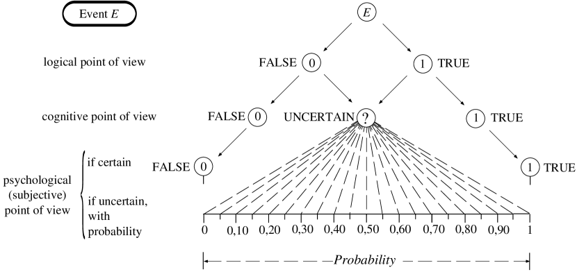
Figure 1: Certain and uncertain events.

So, “what is probability?” Consulting a good dictionary helps. Webster’s states, for example, that “probability is the quality, state, or degree of being probable”, and then that probable means “supported by evidence strong enough to make it likely though not certain to be true”. The concept of probable arises in reasoning when the concept of certain is not applicable. When it is impossible to state firmly if an event (we use this word as a synonym for any possible statement, or proposition, relative to past, present or future) is true or false, we just say that this is possible, probable. Different events may have different levels of probability, depending whether we think that they are more likely to be true or false (see Fig.  1). The concept of probability is then simply

a measure of the degree of belief that an event will occur.

This is the kind of definition that one finds in Bayesian books[3, 4, 5, 6, 7] and the formulation cited here is that given in the ISO “Guide to Expression of Uncertainty in Measurement”[2], of which we will talk later.

At first sight this definition does not seem to be superior to the combinatorial or the frequentistic ones. At least they give some practical rules to calculate “something”. Defining probability as “degree of belief” seems too vague to be of any utility. We need, then, some explanation of its meaning; a tool to evaluate it - and we will look at this tool (Bayes’ theorem) later. We will end this section with some explanatory remarks on the definition, but first let us discuss the advantages of this definition:

• it is natural, very general and it can be applied to any thinkable event, independently of the feasibility of making an inventory of all (equally) possible and favorable cases, or of repeating the experiment under conditions of equal probability;

• it avoids the linguistic schizophrenia of having to distinguish “scientific” probability from “non scientific” probability used in everyday reasoning (though a meteorologist might feel offended to hear that evaluating the probability of rain tomorrow is “not scientific”);

• as far as measurements are concerned, it allows us to talk about the probability of the true value of a physical quantity. In the frequentistic frame it is only possible to talk about the probability of the outcome of an experiment, as the true value is considered to be a constant. This approach is so unnatural that most physicists speak of “$95\,\%$ probability that the mass of the Top quark is between $\ldots$”, although they believe that the correct definition of probability is the limit of the frequency;

• it is possible to make a very general theory of uncertainty which can take into account any source of statistical and systematic error, independently of their distribution.

To get a better understanding of the subjective definition of probability let us take a look at odds in betting. The higher the degree of belief that an event will occur, the higher the amount of money $A$ that someone (“a rational better”) is ready to pay in order to receive a sum of money $B$ if the event occurs. Clearly the bet must be acceptable (“coherent” is the correct adjective), i.e. the amount of money $A$ must be smaller or equal to $B$ and not negative (who would accept such a bet?). The cases of $A=0$ and $A=B$ mean that the events are considered to be false or true, respectively, and obviously it is not worth betting on certainties. They are just limit cases, and in fact they can be treated with standard logic. It seems reasonable that the amount of money $A$ that one is willing to pay grows linearly with the degree of belief. It follows that if someone thinks that the probability of the event $E$ is $p$, then he will bet $A=pB$ to get $B$ if the event occurs, and to lose $pB$ if it does not. It is easy to demonstrate that the condition of “coherence” implies that $0\leq p\leq 1$.

What has gambling to do with physics? The definition of probability through betting odds has to be considered operational, although there is no need to make a bet (with whom?) each time one presents a result. It has the important role of forcing one to make an honest assessment of the value of probability that one believes. One could replace money with other forms of gratification or penalization, like the increase or the loss of scientific reputation. Moreover, the fact that this operational procedure is not to be taken literally should not be surprising. Many physical quantities are defined in a similar way. Think, for example, of the text book definition of the electric field, and try to use it to measure $\vec{E}$ in the proximity of an electron. A nice example comes from the definition of a poisonous chemical compound: it would be lethal if ingested. Clearly it is preferable to keep this operational definition at a hypothetical level, even though it is the best definition of the concept.

2.3 Rules of probability

Figure 2: Venn diagrams and set properties.

The subjective definition of probability, together with the condition of coherence, requires that $0\leq p\leq 1$. This is one of the rules which probability has to obey. It is possible, in fact, to demonstrate that coherence yields to the standard rules of probability, generally known as axioms. At this point it is worth clarifying the relationship between the axiomatic approach and the others:

• combinatorial and frequentistic “definitions” give useful rules for evaluating probability, although they do not, as it is often claimed, define the concept;

• in the axiomatic approach one refrains from defining what the probability is and how to evaluate it: probability is just any real number which satisfies the axioms. It is easy to demonstrate that the probabilities evaluated using the combinatorial and the frequentistic prescriptions do in fact satisfy the axioms;

• the subjective approach to probability, together with the coherence requirement, defines what probability is and provides the rules which its evaluation must obey; these rules turn out to be the same as the axioms.

Since everybody is familiar with the axioms and with the analogy $events\Leftrightarrow sets$ (see Tab.  1 and Fig.  2) let us remind ourselves of the rules of probability in this form:

Events	sets
		symbol
event	set	$E$
certain event	sample space	$\Omega$
impossible event	empty set	$\emptyset$
implication	inclusion	$E_{1}\subseteq E_{2}$
	(subset)
opposite event	complementary set	$\overline{E}$     ($E\cup\overline{E}=\Omega$)
(complementary)
logical product (“AND”)	intersection	$E_{1}\cap E_{2}$
logical sum (“OR”)	union	$E_{1}\cup E_{2}$
incompatible events	disjoint sets	$E_{1}\cap E_{2}=\emptyset$
complete class	finite partition	$\left\{\begin{array}[]{l}E_{i}\cap E_{j}=\emptyset\ (i\neq j)\\ \cup_{i}E_{i}=\Omega\end{array}\right.$

Table 1: Events versus sets.

Axiom 1

$0\leq P(E)\leq 1$;

Axiom 2

$P(\Omega)=1$ (a certain event has probability 1);

Axiom 3

$P(E_{1}\cup E_{2})=P(E_{1})+P(E_{2})$, if $E_{1}\cap E_{2}=\emptyset$

From the basic rules the following properties can be derived:

1:

$P(E)=1-P(\overline{E})$;

2:

$P(\emptyset)=0$;

3:

if $A\subseteq B$ then $P(A)\leq P(B)$;

4:

$P(A\cup B)=P(A)+P(B)-P(A\cap B)$ .

We also anticipate here a fifth property which will be discussed in section  3.1:

5:

$P(A\cap B)=P(A|B)\cdot P(B)=P(A)\cdot P(B|A)\,.$

2.4 Subjective probability and “objective”description of the physical world

The subjective definition of probability seems to contradict the aim of physicists to describe the laws of Physics in the most objective way (whatever this means $\ldots$). This is one of the reasons why many regard the subjective definition of probability with suspicion (but probably the main reason is because we have been taught at University that “probability is frequency”). The main philosophical difference between this concept of probability and an objective definition that “we would have liked” (but which does not exist in reality) is the fact that $P(E)$ is not an intrinsic characteristic of the event $E$, but depends on the status of information available to whoever evaluates $P(E)$. The ideal concept of “objective” probability is recovered when everybody has the “same” status of information. But even in this case it would be better to speak of intersubjective probability. The best way to convince ourselves about this aspect of probability is to try to ask practical questions and to evaluate the probability in specific cases, instead of seeking refuge in abstract questions. I find, in fact, that, paraphrasing a famous statement about Time, “Probability is objective as long as I am not asked to evaluate it”. Some examples:

Example 1:

“What is the probability that a molecule of nitrogen at atmospheric pressure and room temperature has a velocity between 400 and 500 m/s?”. The answer appears easy: “take the Maxwell distribution formula from a text book, calculate an integral and get a number. Now let us change the question: “I give you a vessel containing nitrogen and a detector capable of measuring the speed of a single molecule and you set up the apparatus. Now, what is the probability that the first molecule that hits the detector has a velocity between 400 and 500 m/s?”. Anybody who has minimal experience (direct or indirect) of experiments would hesitate before answering. He would study the problem carefully and perform preliminary measurements and checks. Finally he would probably give not just a single number, but a range of possible numbers compatible with the formulation of the problem. Then he starts the experiment and eventually, after 10 measurements, he may form a different opinion about the outcome of the eleventh measurement.

Example 2:

“What is the probability that the gravitational constant $G_{N}$ has a value between $6.6709\cdot 10^{-11}$ and $6.6743\cdot 10^{-11}$ $\mbox{m}^{3}\mbox{kg}^{-1}\mbox{s}^{-2}$?”. Last year you could have looked at the latest issue of the Particle Data Book[8] and answered that the probability was $95\,\%$. Since then - as you probably know - three new measurements of $G_{N}$ have been performed[9] and we now have four numbers which do not agree with each other (see Tab. 2). The probability of the true value of $G_{N}$ being in that range is currently dramatically decreased.

Institut	$G_{N}$ $\left(10^{-11}\frac{\mbox{m}^{3}}{\mbox{kg}\cdot\mbox{s}^{2}}\right)$	$\frac{\sigma(G_{N})}{G_{N}}$ (ppm)	$\frac{G_{N}-G_{N}^{C}}{G_{N}^{C}}$ ($10^{-3}$)
CODATA 1986 (“$G_{N}^{C}$”)	$6.6726\pm 0.0009$	128	–
PTB (Germany) 1994	$6.7154\pm 0.0006$	83	$+6.41\pm 0.16$
MSL (New Zealand) 1994	$6.6656\pm 0.0006$	95	$-1.05\pm 0.16$
Uni-Wuppertal	$6.6685\pm 0.0007$	105	$-0.61\pm 0.17$
(Germany) 1995

Table 2: Measurement of $G_{N}$ (see text).

Example 3:

“What is the probability that the mass of the Top quark, or that of any of the supersymmetric particles, is below 20 or $50\,\mbox{GeV}/c^{2}$?”. Currently it looks as if it must be zero. Ten years ago many experiments were intensively looking for these particles in those energy ranges. Because so many people where searching for them, with enormous human and capital investment, it means that, at that time, the probability was considered rather high, $\ldots$ high enough for fake signals to be reported as strong evidence for them.

The above examples show how the evaluation of probability is conditioned by some a priori (“theoretical”) prejudices and by some facts (“experimental data”). “Absolute” probability makes no sense. Even the classical example of probability $1/2$ for each of the results in tossing a coin is only acceptable if: the coin is regular; it does not remain vertical (not impossible when playing on the beach); it does not fall into a manhole; etc.

The subjective point of view is expressed in a provocative way by de Finetti’s[5]

“PROBABILITY DOES NOT EXIST”.

3 Conditional probability and Bayes’ theorem

3.1 Dependence of the probability from the status of information

If the status of information changes, the evaluation of the probability also has to be modified. For example most people would agree that the probability of a car being stolen depends on the model, age and parking site. To take an example from physics, the probability that in a HERA detector a charged particle of $1\,\mbox{GeV}$ gives a certain number of ADC counts due to the energy loss in a gas detector can be evaluated in a very general way - using High Energy Physics jargon - making a (huge) Monte Carlo simulation which takes into account all possible reactions (weighted with their cross sections), all possible backgrounds, changing all physical and detector parameters within reasonable ranges, and also taking into account the trigger efficiency. The probability changes if one knows that the particle is a $K^{+}$: instead of very complicated Monte Carlo one can just run a single particle generator. But then it changes further if one also knows the exact gas mixture, pressure, $\ldots$, up to the latest determination of the pedestal and the temperature of the ADC module.

3.2 Conditional probability

Although everybody knows the formula of conditional probability, it is useful to derive it here. The notation is $P(E|H)$, to be read “probability of $E$ given $H$”, where $H$ stands for hypothesis. This means: the probability that $E$ will occur if one already knows that $H$ has occurred.

The event $E|H$ can have three values:

TRUE:

if $E$ is TRUE and $H$ is TRUE;

FALSE:

if $E$ is FALSE and $H$ is TRUE;

UNDETERMINED:

if $H$ is FALSE; in this case we are merely uninterested as to what happens to $E$. In terms of betting, the bet is invalidated and none loses or gains.

Then $P(E)$ can be written $P(E|\Omega)$, to state explicitly that it is the probability of $E$ whatever happens to the rest of the world ($\Omega$ means all possible events). We realize immediately that this condition is really too vague and nobody would bet a cent on a such a statement. The reason for usually writing $P(E)$ is that many conditions are implicitly - and reasonably - assumed in most circumstances. In the classical problems of coins and dice, for example, one assumes that they are regular. In the example of the energy loss, it was implicit -“obvious”- that the High Voltage was on (at which voltage?) and that HERA was running (under which condition?). But one has to take care: many riddles are based on the fact that one tries to find a solution which is valid under more strict conditions than those explicitly stated in the question (e.g. many people make bad business deals signing contracts in which what “was obvious” was not explicitly stated).

In order to derive the formula of conditional probability let us assume for a moment that it is reasonable to talk about “absolute probability” $P(E)=P(E|\Omega)$, and let us rewrite

$$P(E)\equiv P(E|\Omega) \underset{\bf a}{=} P(E\cap\Omega)$$ (1)

$$\underset{\bf b}{=} P\left(E\cap(H\cup\overline{H})\right)$$

$$\underset{\bf c}{=} P\left((E\cap H)\cup(E\cap\overline{H})\right)$$

$$\underset{\bf d}{=} P(E\cap H)+P(E\cap\overline{H})\,,$$

where the result has been achieved through the following steps:

(a):

$E$ implies $\Omega$ (i.e. $E\subseteq\Omega$) and hence $E\cap\Omega=E$;

(b):

the complementary events $H$ and $\overline{H}$ make a finite partition of $\Omega$, i.e. $H\cup\overline{H}=\Omega$;

(c):

distributive property;

(d):

axiom 3.

The final result of (1) is very simple: $P(E)$ is equal to the probability that $E$ occurs and $H$ also occurs, plus the probability that $E$ occurs but $H$ does not occur. To obtain $P(E|H)$ we just get rid of the subset of $E$ which does not contain $H$ (i.e. $E\cap\overline{H}$) and renormalize the probability dividing by $P(H)$, assumed to be different from zero. This guarantees that if $E=H$ then $P(H|H)=1$. The expression of the conditional probability is finally

$$P(E|H)=\frac{P(E\cap H)}{P(H)}\hskip 28.45274pt(P(H)\neq 0)\,.$$ (2)

In the most general (and realistic) case, where both $E$ and $H$ are conditioned by the occurrence of a third event $H_{\circ}$, the formula becomes

$$P(E|H,H_{\circ})=\frac{P\left(E\cap(H|H_{\circ})\right)}{P(H|H_{\circ})}\hskip 28.45274pt(P(H|H_{\circ})\neq 0)\,.$$ (3)

Usually we shall make use of (2) (which means $H_{\circ}=\Omega$) assuming that $\Omega$ has been properly chosen. We should also remember that (2) can be resolved with respect to $P(E\cap H)$, obtaining the well known

$$P(E\cap H)=P(E|H)P(H)\,,$$ (4)

and by symmetry

$$P(E\cap H)=P(H|E)P(E)\,.$$ (5)

Two events are called independent if

$$P(E\cap H)=P(E)P(H)\,.$$ (6)

This is equivalent to saying that $P(E|H)=P(E)$ and $P(H|E)=P(H)$, i.e. the knowledge that one event has occurred does not change the probability of the other. If $P(E|H)\neq P(E)$ then the events $E$ and $H$ are correlated. In particular:

• if $P(E|H)>P(E)$ then $E$ and $H$ are positively correlated;

• if $P(E|H)<P(E)$ then $E$ and $H$ are negatively correlated;

3.3 Bayes’ theorem

Let us think of all the possible, mutually exclusive, hypotheses $H_{i}$ which could condition the event $E$. The problem here is the inverse of the previous one: what is the probability of $H_{i}$ under the hypothesis that $E$ has occurred? For example, “what is the probability that a charged particle which went in a certain direction and has lost between 100 and $120\,\mbox{keV}$ in the detector, is a $\mu$, a $\pi$, a $K$, or a $p$?” Our event $E$ is “energy loss between 100 and $120\,\mbox{keV}$”, and $H_{i}$ are the four “particle hypotheses”. This example sketches the basic problem for any kind of measurement: having observed an effect, to assess the probability of each of the causes which could have produced it. This intellectual process is called inference, and it will be discussed after section  9.

In order to calculate $P(H_{i}|E)$ let us rewrite the joint probability $P(H_{i}\cap E)$, making use of (4-5), in two different ways:

$$P(H_{i}|E)P(E)=P(E|H_{i})P(H_{i})\,,$$ (7)

obtaining

$$\boxed{P(H_{i}|E)=\frac{P(E|H_{i})P(H_{i})}{P(E)}\,,}$$ (8)

or

$$\boxed{\frac{P(H_{i}|E)}{P(H_{i})}=\frac{P(E|H_{i})}{P(E)}\,.}$$ (9)

Since the hypotheses $H_{i}$ are mutually exclusive (i.e. $H_{i}\cap H_{j}=\emptyset$, $\forall\,i,j$) and exhaustive (i.e. $\bigcup_{i}H_{i}=\Omega$), $E$ can be written as $E\cup H_{i}$, the union of $E$ with each of the hypotheses $H_{i}$. It follows that

$$P(E)\equiv P(E\cap\Omega) = P\left(E\cap\bigcup_{i}H_{i}\right)=P\left(\bigcup_{i}(E\cap H_{i})\right)$$ (10)

$$= \sum_{i}P(E\cap H_{i})$$

$$= \sum_{i}P(E|H_{i})P(H_{i})\,,$$

where we have made use of (4) again in the last step. It is then possible to rewrite (8) as

$$\boxed{P(H_{i}|E)=\frac{P(E|H_{i})P(H_{i})}{\sum_{j}P(E|H_{j})P(H_{j})}\,.}$$ (11)

This is the standard form by which Bayes’ theorem is known. (8) and (9) are also different ways of writing it. As the denominator of (11) is nothing but a normalization factor (such that $\sum_{i}P(H_{i}|E)=1$), the formula (11) can be written as

$$\boxed{P(H_{i}|E)\propto P(E|H_{i})P(H_{i})\,.}$$ (12)

Factorizing $P(H_{i})$ in (11), and explicitly writing the fact that all the events were already conditioned by $H_{\circ}$, we can rewrite the formula as

$$\boxed{P(H_{i}|E,H_{\circ})=\alpha P(H_{i}|H_{\circ})\,,}$$ (13)

with

$$\alpha=\frac{P(E|H_{i},H_{\circ})}{\sum_{i}P(E|H_{i},H_{\circ})P(H_{i}|H_{\circ})}\,.$$ (14)

These five ways of rewriting the same formula simply reflect the importance that we shall give to this simple theorem. They stress different aspects of the same concept:

• (11) is the standard way of writing it (although some prefer (8));

• (9) indicates that $P(H_{i})$ is altered by the condition $E$ with the same ratio with which $P(E)$ is altered by the condition $H_{i}$;

• (12) is the simplest and the most intuitive way to formulate the theorem: ”the probability of $H_{i}$ given $E$ is proportional to the initial probability of $H_{i}$ times the probability of $E$ given $H_{i}$”;

• (13-14) show explicitly how the probability of a certain hypothesis is updated when the status of information changes:

  $P(H_{i}|H_{\circ})$

  (also indicated as $P_{\circ}(H_{i})$) is the initial, or a priori, probability (or simply “prior”) of $H_{i}$, i.e. the probability of this hypothesis with the status of information available before the knowledge that $E$ has occurred;

  $P(H_{i}|E,H_{\circ})$

  (or simply $P(H_{i}|E)$) is the final, or “a posteriori”, probability of $H_{i}$ after the new information;

  $P(E|H_{i},H_{\circ})$

  (or simply $P(E|H_{i})$) is called likelihood.

To better understand the terms “initial”, “final” and “likelihood”, let us formulate the problem in a way closer to the physicist’s mentality, referring to causes and effects: the causes can be all the physical sources which may produce a certain observable (the effect). The likelihoods are - as the word says - the likelihoods that the effect follows from each of the causes. Using our example of the $dE/dx$ measurement again, the causes are all the possible charged particles which can pass through the detector; the effect is the amount of observed ionization; the likelihoods are the probabilities that each of the particles give that amount of ionization. Notice that in this example we have fixed all the other sources of influence: physics process, HERA running conditions, gas mixture, High Voltage, track direction, etc.. This is our $H_{\circ}$. The problem immediately gets rather complicated (all real cases, apart from tossing coins and dice, are complicated!). The real inference would be of the kind

$$P(H_{i}|E,H_{\circ})\propto P(E|H_{i},H_{\circ})P(H_{i}|H_{\circ})P(H_{\circ}),.$$ (15)

For each status of $H_{\circ}$ (the set of all the possible values of the influence parameters) one gets a different result for the final probability. So, instead of getting a single number for the final probability we have a distribution of values. This spread will result in a large uncertainty of $P(H_{i}|E)$. This is what every physicist knows: if the calibration constants of the detector and the physics process are not under control, the “systematic errors” are large and the result is of poor quality.

3.4 Conventional use of Bayes’ theorem

Bayes’ theorem follows directly from the rules of probability, and it can be used in any kind of approach. Let us take an example:

Problem 1:

A particle detector has a $\mu$ identification efficiency of $95\,\%$, and a probability of identifying a $\pi$ as a $\mu$ of $2\,\%$. If a particle is identified as a $\mu$, then a trigger is issued. Knowing that the particle beam is a mixture of $90\,\%$ $\pi$ and $10\,\%$ $\mu$, what is the probability that a trigger is really fired by a $\mu$? What is the signal-to-noise ($S/N$) ratio?

Solution:

The two hypotheses (causes) which could condition the event (effect) $T$ (=“trigger fired”) are “$\mu$” and “$\pi$”. They are incompatible (clearly) and exhaustive (90 %+10 %=100 %). Then:

$$P(\mu|T) = \frac{P(T|\mu)P_{\circ}(\mu)}{P(T|\mu)P_{\circ}(\mu)+P(T|\pi)P_{\circ}(\pi)}$$

$$= \frac{0.95\times 0.1}{0.95\times 0.1+0.02\times 0.9}=0.84\,,$$

and $P(\pi|T)=0.16$.

The signal to noise ratio is $P(\mu|T)/P(\pi|T)=5.3$. It is interesting to rewrite the general expression of the signal to noise ratio if the effect $E$ is observed as

$$S/N=\frac{P(S|E)}{P(N|E)}=\frac{P(E|S)}{P(E|N)}\cdot\frac{P_{\circ}(S)}{P_{\circ}(N)}\,.$$ (17)

This formula explicitly shows that when there are noisy conditions

$$P_{\circ}(S)\ll P_{\circ}(N)$$

the experiment must be very selective

$$P(E|S)\gg P(E|N)$$

in order to have a decent $S/N$ ratio.
(How does the $S/N$ change if the particle has to be identified by two independent detectors in order to give the trigger? Try it yourself, the answer is $S/N=251$.)

Problem 2:

Three boxes contain two rings each, but in one of them they are both gold, in the second both silver, and in the third one of each type. You have the choice of randomly extracting a ring from one of the boxes, the content of which is unknown to you. You look at the selected ring, and you then have the possibility of extracting a second ring, again from any of the three boxes. Let us assume the first ring you extract is a gold one. Is it then preferable to extract the second one from the same or from a different box?

Solution:

Choosing the same box you have a $2/3$ probability of getting a second gold ring. (Try to apply the theorem, or help yourself with intuition.)

The difference between the two problems, from the conventional statistics point of view, is that the first is only meaningful in the frequentistic approach, the second only in the combinatorial one. They are, however, both acceptable from the Bayesian point of view. This is simply because in this framework there is no restriction on the definition of probability. In many and important cases of life and science, neither of the two conventional definitions are applicable.

3.5 Bayesian statistics: learning by experience

The advantage of the Bayesian approach (leaving aside the “little philosophical detail” of trying to define what probability is) is that one may talk about the probability of any kind of event, as already emphasized. Moreover, the procedure of updating the probability with increasing information is very similar to that followed by the mental processes of rational people. Let us consider a few examples of “Bayesian use” of Bayes’ theorem:

Example 1:

Imagine some persons listening to a common friend having a phone conversation with an unknown person $X_{i}$, and who are trying to guess who $X_{i}$ is. Depending on the knowledge they have about the friend, on the language spoken, on the tone of voice, on the subject of conversation, etc., they will attribute some probability to several possible persons. As the conversation goes on they begin to consider some possible candidates for $X_{i}$, discarding others, and eventually fluctuating between two possibilities, until the status of information $I$ is such that they are practically sure of the identity of $X_{i}$. This experience has happened to must of us, and it is not difficult to recognize the Bayesian scheme:

$$P(X_{i}|I,I_{\circ})\propto P(I|X_{i},I_{\circ})P(X_{i}|I_{\circ})\,.$$ (18)

We have put the initial status of information $I_{\circ}$ explicitly in (18) to remind us that likelihoods and initial probabilities depend on it. If we know nothing about the person, the final probabilities will be very vague, i.e. for many persons $X_{i}$ the probability will be different from zero, without necessarily favoring any particular person.

Example 2:

A person $X$ meets an old friend $F$ in a pub. $F$ proposes that the drinks should be payed for by whichever of the two extracts the card of lower value from a pack (according to some rule which is of no interest to us). $X$ accepts and $F$ wins. This situation happens again in the following days and it is always $X$ who has to pay. What is the probability that $F$ has become a cheat, as the number of consecutive wins $n$ increases?

The two hypotheses are: cheat ($C$) and honest ($H$). $P_{\circ}(C)$ is low because $F$ is an “old friend”, but certainly not zero (you know $\ldots$): let us assume $5\,\%$. To make the problem simpler let us make the approximation that a cheat always wins (not very clever$\ldots$): $P(W_{n}|C)=1)$. The probability of winning if he is honest is, instead, given by the rules of probability assuming that the chance of winning at each trial is $1/2$ (”why not?”, we shall come back to this point later): $P(W_{n}|H)=2^{-n}$. The result

$$P(C|W_{n}) = \frac{P(W_{n}|C)\cdot P_{\circ}(C)}{P(W_{n}|C)\cdot P_{\circ}(C)+P(W_{n}|H)\cdot P_{\circ}(H)}$$ (19)

$$= \frac{1\cdot P_{\circ}(C)}{1\cdot P_{\circ}(C)+2^{-n}\cdot P_{\circ}(H)}$$

is shown in the following table:

$n$	$P(C|W_{n})$	$P(H|W_{n})$
	(%)	(%)
0	5.0	95.0
1	9.5	90.5
2	17.4	82.6
3	29.4	70.6
4	45.7	54.3
5	62.7	37.3
6	77.1	22.9
$\ldots$	$\ldots$	$\ldots$

Naturally, as $F$ continues to win the suspicion of $X$ increases. It is important to make two remarks:

• the answer is always probabilistic. $X$ can never reach absolute certainty that $F$ is a cheat, unless he catches $F$ cheating, or $F$ confesses to having cheated. This is coherent with the fact that we are dealing with random events and with the fact that any sequence of outcomes has the same probability (although there is only one possibility over $2^{n}$ in which $F$ is always luckier). Making use of $P(C|W_{n})$, $X$ can take a decision about the next action to take:

  • continue the game, with probability $P(C|W_{n})$ of losing, with certainty, the next time too;

  • refuse to play further, with probability $P(H|W_{n})$ of offending the innocent friend.

• If $P_{\circ}(C)=0$ the final probability will always remain zero: if $X$ fully trusts $F$, then he has just to record the occurrence of a rare event when $n$ becomes large.

To better follow the process of updating the probability when new experimental data become available, according to the Bayesian scheme

“the final probability of the present inference is the initial probability of the next one” ,

let us call $P(C|W_{n-1})$ the probability assigned after the previous win. The iterative application of the Bayes formula yields:

$$P(C|W_{n}) = \frac{P(W|C)\cdot P(C|W_{n-1})}{P(W|C)\cdot P(C|W_{n-1})+P(W|H)\cdot P(H|W_{n-1})}$$ (20)

$$= \frac{1\cdot P(C|W_{n-1})}{1\cdot P(C|W_{n-1})+\frac{1}{2}\cdot P(H|W_{n-1})}\,,$$

where $P(W|C)=1$ and $P(W|H)=1/2$ are the probabilities of each win. The interesting result is that exactly the same values of $P(C|W_{n})$ of (19) are obtained (try to believe it!).

It is also instructive to see the dependence of the final probability on the initial probabilities, for a given number of wins $n$:

	$P(C|W_{n})$
$P_{\circ}(C)$	$(\%)$
	$n=5$	$n=10$	$n=15$	$n=20$
$1\,\%$	24	91	99.7	99.99
$5\,\%$	63	98	99.94	99.998
$50\,\%$	97	99.90	99.997	99.9999

As the number of experimental observations increases the conclusions no longer depend, practically, on the initial assumptions. This is a crucial point in the Bayesian scheme and it will be discussed in more detail later.

4 Hypothesis test (discrete case)

Although in conventional statistics books this argument is usually dealt with in one of the later chapters, in the Bayesian approach this is so natural that it is in fact the first application, as we have seen in the above examples. We summarize here the procedure:

• probabilities are attributed to the different hypotheses using initial probabilities and experimental data (via the likelihood);

• the person who makes the inference - or the “user” - will take a decision of which he is fully responsible.

If one needs to compare two hypotheses, as in the example of the signal to noise calculation, the ratio of the final probabilities can be taken as a quantitative result of the test. Let us rewrite the $S/N$ formula in the most general case:

$$\frac{P(H_{1}|E,H_{\circ})}{P(H_{2}|E,H_{\circ})}=\frac{P(E|H_{1},H_{\circ})}{P(E|H_{2},H_{\circ})}\cdot\frac{P(H_{1}|H_{\circ})}{P(H_{2}|H_{\circ})}\,,$$ (21)

where again we have reminded ourselves of the existence of $H_{\circ}$. The ratio depends on the product of two terms: the ratio of the priors and the ratio of the likelihoods. When there is absolutely no reason for choosing between the two hypotheses the prior ratio is 1 and the decision depends only on the other term, called the Bayes factor. If one firmly believes in either hypothesis, the Bayes factor is of minor importance, unless it is zero or infinite (i.e. one and only one of the likelihoods is vanishing). Perhaps this is disappointing for those who expected objective certainties from a probability theory, but this is in the nature of things.

5 Choice of the initial probabilities (discrete case)

5.1 General criteria

The dependence of Bayesian inferences on initial probability is pointed to by opponents as the fatal flaw in the theory. But this criticism is less severe than one might think at first sight. In fact:

• It is impossible to construct a theory of uncertainty which is not affected by this “illness”. Those methods which are advertised as being “objective” tend in reality to hide the hypotheses on which they are grounded. A typical example is the maximum likelihood method, of which we will talk later.

• as the amount of information increases the dependence on initial prejudices diminishes;

• when the amount of information is very limited, or completely lacking, there is nothing to be ashamed of if the inference is dominated by a priori assumptions;

The fact that conclusions drawn from an experimental result (and sometimes even the “result” itself!) often depend on prejudices about the phenomenon under study is well known to all experienced physicists. Some examples:

• when doing quick checks on a device, a single measurement is usually performed if the value is “what it should be”, but if it is not then many measurements tend to be made;

• results are sometimes influenced by previous results or by theoretical predictions. See for example Fig.  3 taken from the Particle Data Book[8]. The interesting book “How experiments end”[10] discusses, among others, the issue of when experimentalists are “happy with the result” and stop “correcting for the systematics”;

• it can happen that slight deviations from the background are interpreted as a signal (e.g. as for the first claim of discovery of the Top quark in spring ’94), while larger “signals” are viewed with suspicion if they are unwanted by the physics “establishment”;

• experiments are planned and financed according to the prejudices of the moment;

Figure 3: Results on two physical quantities as a function of the publication date.

These comments are not intended to justify unscrupulous behaviour or sloppy analysis. They are intended, instead, to remind us - if need be - that scientific research is ruled by subjectivity much more than outsiders imagine. The transition from subjectivity to “objectivity” begins when there is a large consensus among the most influential people about how to interpret the results.

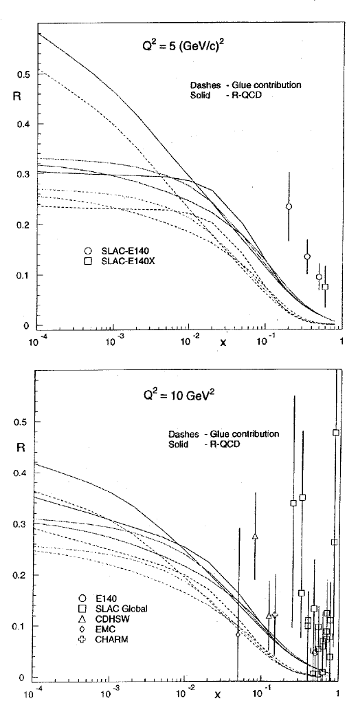
Figure 4: $R=\sigma_{L}/\sigma_{T}$ as a function of the Deep Inelastic Scattering variable $x$ as measured by experiments and as predicted by QCD.

In this context, the subjective approach to statistical inference at least teaches us that every assumption must be stated clearly and all available information which could influence conclusions must be weighed with the maximum attempt at objectivity.

What are the rules for choosing the “right” initial probabilities? As one can imagine, this is an open and debated question among scientists and philosophers. My personal point of view is that one should avoid pedantic discussion of the matter, because the idea of universally true priors reminds me terribly of the famous “angels’ sex” debates.

If I had to give recommendations, they would be:

• the a priori probability should be chosen in the same spirit as the rational person who places a bet, seeking to minimize the risk of losing;

• general principles - like those that we will discuss in a while - may help, but since it may be difficult to apply elegant theoretical ideas in all practical situations, in many circumstances the guess of the “expert” can be relied on for guidance.

• avoid using as prior the results of other experiments dealing with the same open problem, otherwise correlations between the results would prevent all comparison between the experiments and thus the detection of any systematic errors. I find that this point is generally overlooked by statisticians.

5.2 Insufficient Reason and Maximum Entropy

The first and most famous criterion for choosing initial probabilities is the simple Principle of Insufficient Reason (or Indifference Principle): if there is no reason to prefer one hypothesis over alternatives, simply attribute the same probability to all of them. This was stated as a principle by Laplace in contrast to Leibnitz’ famous Principle of Sufficient Reason, which, in simple words, states that ”nothing happens without a reason”. The indifference principle applied to coin and die tossing, to card games or to other simple and symmetric problems, yields to the well known rule of probability evaluation that we have called combinatorial. Since it is impossible not to agree with this point of view, in the cases that one judges that it does apply, the combinatorial “definition” of probability is recovered in the Bayesian approach if the word “definition” is simply replaced by “evaluation rule”. We have in fact already used this reasoning in previous examples.

A modern and more sophisticated version of the Indifference Principle is the Maximum Entropy Principle. The information entropy function of $n$ mutually exclusive events, to each of which a probability $p_{i}$ is assigned, is defined as

$$H(p_{1},p_{2},\ldots p_{n})=-K\sum_{i=1}^{n}p_{i}\ln{p_{i}},$$ (22)

with $K$ a positive constant. The principle states that “in making inferences on the basis of partial information we must use that probability distribution which has the maximum entropy subject to whatever is known[13]”. Notice that, in this case, “entropy” is synonymous with “uncertainty”[13]. One can show that, in the case of absolute ignorance about the events $E_{i}$, the maximization of the information uncertainty, with the constraint that $\sum_{i=1}^{n}p_{i}=1$, yields the classical $p_{i}=1/n$ (any other result would have been worrying$\ldots$).

Although this principle is sometimes used in combination with the Bayes’ formula for inferences (also applied to measurement uncertainty, see [14]), it will not be used for applications in these notes.

6 Random variables

In the discussion which follows I will assume that the reader is familiar with random variables, distributions, probability density functions, expected values, as well as with the most frequently used distributions. This section is only intended as a summary of concepts and as a presentation of the notation used in the subsequent sections.

6.1 Discrete variables

Stated simply, to define a random variable $X$ means to find a rule which allows a real number to be related univocally (but not biunivocally) to an event ($E$), chosen from those events which constitute a finite partition of $\Omega$ (i.e. the events must be exhaustive and mutually exclusive). One could write this expression $X(E)$. If the number of possible events is finite then the random variable is discrete, i.e. it can assume only a finite number of values. Since the chosen set of events are mutually exclusive, the probability of $X=x$ is the sum of the probabilities of all the events for which $X(E_{i})=x$. Note that we shall indicate the variable with $X$ and its numerical realization with $x$, and that, differently from other notations, the symbol $x$ (in place of $n$ or $k$) is also used for discrete variables.

After this short introduction, here is a list of definitions, properties and notations:

Probability function:

$$f(x)=P(X=x)\,.$$ (23)

It has the following properties:

$$1) 0\leq f(x_{i})\leq 1\,;$$ (24)

$$2) P(X=x_{i}\,\cup\,X=x_{j})=f(x_{i})+f(x_{j})\,;$$ (25)

$$3) \sum_{i}f(x_{i})=1\,.$$ (26)

Cumulative distribution function:

$$F(x_{k})\equiv P(X\leq x_{k})=\sum_{x_{i}\leq x_{k}}f(x_{i})\,.$$ (27)

Properties:

$$1) F(-\infty)=0$$ (28)

$$2) F(+\infty)=1$$ (29)

$$3) F(x_{i})-F(x_{i-1})=f(x_{i})$$ (30)

$$4) \lim_{\epsilon\rightarrow o}F(x+\epsilon)=F(x)\hskip 28.45274pt(right\ side\ continuity)\,.$$ (31)

Expected value (mean):

$$\mu\equiv E[X]=\sum_{i}x_{i}f(x_{i})\,.$$ (32)

In general, given a function $g(X)$ of $X$:

$$E[g(X)]=\sum_{i}g(x_{i})f(x_{i})\,.$$ (33)

$E[\cdot]$ is a linear operator:

$$E[aX+b]=aE[X]+b\,.$$ (34)

Variance and standard deviation:

Variance:

$$\sigma^{2}\equiv Var(X)=E[(X-\mu)^{2}]=E[X^{2}]-\mu^{2}\,.$$ (35)

Standard deviation:

$$\sigma=+\sqrt{\sigma^{2}}\,.$$ (36)

Transformation properties:

$$Var(aX+b) = a^{2}Var(X)\,;$$ (37)

$$\sigma(aX+b) = |a|\sigma(X)\,.$$ (38)

Binomial distribution:

$X\sim{\cal B}_{n,p}$ (hereafter “$\sim$” stands for “follows”); ${\cal B}_{n,p}$ stands for binomial with parameters $n$ (integer) and $p$ (real):

$$f(x|{\cal B}_{n,p})=\frac{n!}{(n-x)!x!}p^{x}(1-p)^{n-x}\,,\hskip 28.45274pt\left\{\begin{array}[]{l}n=1,2,\ldots,\infty\\ 0\leq p\leq 1\\ x=0,1,\ldots,n\end{array}\right.\,.$$ (39)

Expected value, standard deviation and variation coefficient:

$$\mu = np$$ (40)

$$\sigma = \sqrt{np(1-p)}$$ (41)

$$v\equiv\frac{\sigma}{\mu} = \frac{\sqrt{np(1-p)}}{np}\propto\frac{1}{\sqrt{n}}\,.$$ (42)

$1-p$ is often indicated by $q$.

Poisson distribution:

$X\sim{\cal P}_{\lambda}$:

$$f(x|{\cal P}_{\lambda})=\frac{\lambda^{x}}{x!}e^{-\lambda}\hskip 28.45274pt\left\{\begin{array}[]{l}0<\lambda<\infty\\ x=0,1,\ldots,\infty\\ \end{array}\right.\,.$$ (43)

($x$ is integer, $\lambda$ is real.)
Expected value, standard deviation and variation coefficient:

$$\mu = \lambda$$ (44)

$$\sigma = \sqrt{\lambda}$$ (45)

$$v = \frac{1}{\sqrt{\lambda}}$$ (46)

Binomial $\rightarrow$ Poisson:

$${\cal B}_{n,p}@>>{\begin{array}[]{l}n\rightarrow``\infty^{\prime\prime}\\ p\rightarrow``0^{\prime\prime}\\ (\lambda=np)\end{array}}>{\cal P}_{\lambda}\,.$$ (47)

6.2 Continuous variables: probability and density function

Moving from discrete to continuous variables there are the usual problems with infinite possibilities, similar to those found in Zeno’s “Achilles and the tortoise” paradox. In both cases the answer is given by infinitesimal calculus. But some comments are needed:

• the probability of each of the realizations of $X$ is zero ($P(X=x)=0$), but this does not mean that each value is impossible, otherwise it would be impossible to get any result;

• although all values $x$ have zero probability, one usually assigns different degrees of belief to them, quantified by the probability density function $f(x)$. Writing $f(x_{1})>f(x_{2})$, for example, indicates that our degree of belief in $x_{1}$ is greater than that in $x_{2}$.

• The probability that a random variable lies inside a finite interval, for example $P(a\leq X\leq b)$, is instead finite. If the distance between $a$ and $b$ becomes infinitesimal, then the probability becomes infinitesimal too. If all the values of $X$ have the same degree of belief (and not only equal numerical probability $P(x)=0$) the infinitesimal probability is simply proportional to the infinitesimal interval $dP=kdx$. In the general case the ratio between two infinitesimal probabilities around two different points will be equal to the ratio of the degrees of belief in the points (this argument implies the continuity of $f(x)$ on either side of the values). It follows that $dP=f(x)dx$ and then

  $$P(a\leq X\leq b)=\int_{a}^{b}f(x)dx\,;$$ (48)

• $f(x)$ has a dimension inverse to that of the random variable.

After this short introduction, here is a list of definitions, properties and notations:

Cumulative distribution function:

$$F(x)=P(X\leq x)=\int_{-\infty}^{x}f(x^{\prime})dx^{\prime}\,,$$ (49)

or

$$f(x)=\frac{dF(x)}{dx}$$ (50)

Properties of $f(x)$ and $F(x)$:

• $f(x)\geq 0\,\,$;

• $\int_{-\infty}^{+\infty}f(x)dx=1\,\,$;

• $0\leq F(x)\leq 1$;

• $P(a\leq X\leq b)=\int_{a}^{b}f(x)dx=\int_{-\infty}^{b}f(x)dx-\int_{-\infty}^{a}f(x)dx\\ \hskip 75.11525pt=F(b)-F(a)$;

• if $x_{2}>x_{1}$ then $F(x_{2})\geq F(x_{1})$ .

• $\lim_{x\rightarrow-\infty}F(x)=0$ ;
  $\lim_{x\rightarrow+\infty}F(x)=1$ ;

Expected value:

$$E[X] = \int_{-\infty}^{+\infty}xf(x)dx$$ (51)

$$E[g(X)] = \int_{-\infty}^{+\infty}g(x)f(x)dx.$$ (52)

Uniform distribution:

​ $X\sim{\cal K}(a,b)$:

$$f(x|{\cal K}(a,b)) = \frac{1}{b-a}\hskip 17.07182pt(a\leq x\leq b)$$ (53)

$$F(x|{\cal K}(a,b)) = \frac{x-a}{b-a}\,.$$ (54)

Expected value and standard deviation:

$$\mu = \frac{a+b}{2}$$ (55)

$$\sigma = \frac{b-a}{\sqrt{12}}\,.$$ (56)

Normal (gaussian) distribution:

$X\sim{\cal N}(\mu,\sigma)$:

$$f(x|{\cal N}(\mu,\sigma))=\frac{1}{\sqrt{2\pi}\sigma}e^{-\frac{(x-\mu)^{2}}{2\sigma^{2}}}\hskip 28.45274pt\left\{\begin{array}[]{l}-\infty<\mu<+\infty\\ 0<\sigma<\infty\\ -\infty<x<+\infty\end{array}\right.\,,$$ (57)

where $\mu$ and $\sigma$ (both real) are the expected value and standard deviation, respectively.

Standard normal distribution:

the particular normal distribution of mean 0 and standard deviation 1, usually indicated by $Z$:

$$Z\sim{\cal N}(0,1)\,.$$ (58)

Exponential distribution:

$T\sim{\cal E}(\tau)$:

$$f(t|{\cal E}(\tau)) = \frac{1}{\tau}e^{-t/\tau}\hskip 36.98866pt\left\{\begin{array}[]{c}0\leq\tau<\infty\\ 0\leq t<\infty\end{array}\right.$$ (61)

$$F(t|{\cal E}(\tau)) = 1-e^{-t/\tau}$$ (62)

we use of the symbol $t$ instead of $x$ because this distribution will be applied to the time domain.
Survival probability:

$$P(T>t)=1-F(t|{\cal E}(\tau))=e^{-t/\tau}$$ (63)

Expected value and standard deviation:

$$\mu = \tau$$ (64)

$$\sigma = \tau.$$ (65)

The real parameter $\tau$ has the physical meaning of lifetime.

Poisson $\leftrightarrow$ Exponential:

If $X$ (= “number of counts during the time $\Delta t$”) is Poisson distributed then $T$ (=“interval of time to be waited - starting from any instant - before the first count is recorded”) is exponentially distributed:

$$X\sim f(x|{\cal P}_{\lambda}) \Longleftrightarrow T\sim f(x|{\cal E}(\tau))$$ (66)

$$(\tau=\frac{\Delta T}{\lambda})$$ (67)

6.3 Distribution of several random variables

We only consider the case of two continuous variables ($X$ and $Y$). The extension to more variables is straightforward. The infinitesimal element of probability is $dF(x,y)=f(x,y)dxdy$, and the probability density function

$$f(x,y)=\frac{\partial^{2}F(x,y)}{\partial x\partial y}\,.$$ (68)

The probability of finding the variable inside a certain area $A$ is

$$\iint\limits_{A}f(x,y)dxdy\,.$$ (69)

Marginal distributions:

$$f_{X}(x) = \int_{-\infty}^{+\infty}f(x,y)dy$$ (70)

$$f_{Y}(y) = \int_{-\infty}^{+\infty}f(x,y)dx\,.$$ (71)

The subscripts $X$ and $Y$ indicate that $f_{X}(x)$ and $f_{Y}(y)$ are only function of $X$ and $Y$, respectively (to avoid fooling around with different symbols to indicate the generic function).

Conditional distributions:

$$f_{X}(x|y) = \frac{f(x,y)}{f_{Y}(y)}=\frac{f(x,y)}{\int f(x,y)dx}$$ (72)

$$f_{Y}(y|x) = \frac{f(x,y)}{f_{X}(x)}$$ (73)

$$f(x,y) = f_{X}(x|y)f_{Y}(y)$$ (74)

$$= f_{Y}(y|x)f_{Y}(x)\,.$$ (75)

Independent random variables

$$f(x,y)=f_{X}(x)f_{Y}(y)$$ (76)

(it implies $f(x|y)=f_{X}(x)$ and $f(y|x)=f_{Y}(y)$ .)

Bayes’ theorem for continuous random variables

$$\boxed{f(h|e)=\frac{f(e|h)f_{h}(h)}{\int f(e|h)f_{h}(h)dh}\,.}$$ (77)

Expected value:

$$\mu_{X}=E[X] = \int\!\!\int_{-\infty}^{+\infty}\!xf(x,y)dxdy$$ (78)

$$= \int_{-\infty}^{+\infty}\!xf_{X}(x)dx\,,$$ (79)

and analogously for $Y$. In general

$$E[g(X,Y)]=\int\!\!\int_{-\infty}^{+\infty}\!g(x,y)f(x,y)dxdy\,.$$ (80)

Variance:

$$\sigma_{X}^{2}=E[X^{2}]-E^{2}[X]\,,$$ (81)

and analogously for $Y$.

Covariance:

$$Cov(X,Y) = E\left[\left(X-E[X]\right)\left(Y-E[Y]\right)\right]$$ (82)

$$= E[XY]-E[X]E[Y]\,.$$ (83)

If $Y$ and $Y$ are independent, then $E[XY]=E[X]E[Y]$ and hence $Cov(X,Y)=0$ (the opposite is true only if $X$, $Y\sim{\cal N}(\cdot)$).

Correlation coefficient:

$$\rho(X,Y) = \frac{Cov(X,Y)}{\sqrt{Var(X)Var(Y)}}$$ (84)

$$= \frac{Cov(X,Y)}{\sigma_{X}\sigma_{Y}}\,.$$ (85)

$$(-1\leq\rho\leq 1)$$

Linear combinations of random variables:

If $Y=\sum_{i}c_{i}X_{i}$, with $c_{i}$ real, then:

$$\mu_{Y}=E[Y] = \sum_{i}c_{i}E[X_{i}]=\sum_{i}c_{i}\mu_{i}$$ (86)

$$\sigma_{Y}^{2}=Var(Y) = \sum_{i}c_{i}^{2}Var(X_{i})+2\sum_{i<j}c_{i}c_{j}Cov(X_{i},X_{j})$$ (87)

$$= \sum_{i}c_{i}^{2}Var(X_{i})+\sum_{i\neq j}c_{i}c_{j}Cov(X_{i},X_{j})$$ (88)

$$= \sum_{i}c_{i}^{2}\sigma_{i}^{2}+\sum_{i\neq j}\rho_{ij}c_{i}c_{j}\sigma_{i}\sigma_{j}$$ (89)

$$= \sum_{ij}\rho_{ij}c_{i}c_{j}\sigma_{i}\sigma_{j}$$ (90)

$$= \sum_{ij}c_{i}c_{j}\sigma_{ij}\,.$$ (91)

$\sigma^{2}_{Y}$ has been written in the different ways, with increasing levels of compactness, that can be found in the literature. In particular, (91) uses the convention $\sigma_{ii}=\sigma^{2}_{i}$ and the fact that, by definition, $\rho_{ii}=1$.

Bivariate normal distribution:

joint probability density function of $X$ and $Y$ with correlation coefficient $\rho$ (see Fig  5):

Figure 5: Example of bivariate normal distribution.

$$f(x,y) = \frac{1}{2\pi\sigma_{x}\sigma_{y}\sqrt{1-\rho^{2}}}\cdot$$

$$\exp{\left\{-\frac{1}{2(1-\rho^{2})}\left[\frac{(x-\mu_{x})^{2}}{\sigma_{x}^{2}}-2\rho\frac{(x-\mu_{x})(y-\mu_{y})}{\sigma_{x}\sigma_{y}}+\frac{(y-\mu_{y})^{2}}{\sigma_{y}^{2}}\right]\right\}}\,.$$

Marginal distributions:

$$X \sim {\cal N}(\mu_{x},\sigma_{x})$$ (93)

$$Y \sim {\cal N}(\mu_{y},\sigma_{y})\,.$$ (94)

Conditional distribution:

$$f(y|x_{\circ})=\frac{1}{\sqrt{2\pi}\sigma_{y}\sqrt{1-\rho^{2}}}\exp{\left[-\frac{\left(y-\left[\mu_{y}+\rho\frac{\sigma_{y}}{\sigma_{x}}\left(x_{\circ}-\mu_{x}\right)\right]\right)^{2}}{2\sigma_{y}^{2}(1-\rho^{2})}\right]}\,,$$ (95)

i.e.

$$Y_{|x_{\circ}}\sim{\cal N}\left(\mu_{y}+\rho\frac{\sigma_{y}}{\sigma_{x}}\left(x_{\circ}-\mu_{x}\right),\,\sigma_{y}\sqrt{1-\rho^{2}}\right):$$ (96)

the condition $X=x_{\circ}$ squeezes the standard deviation and shifts the mean of $Y$.

7 Central limit theorem

7.1 Terms and role

Figure 6: Central limit theorem at work: the sum of $n$ variables, for two different distribution, is shown. The values of $n$ (top-down) are: 1,2,3,5,10,20,50.

The well known central limit theorem plays a crucial role in statistics and justifies the enormous importance that the normal distribution has in many practical applications (this is the reason why it appears on 10 DM notes).

We have reminded ourselves in (86-87) of the expression of the mean and variance of a linear combination of random variables

$$Y=\sum_{i=1}^{n}X_{i}$$

in the most general case, which includes correlated variables ($\rho_{ij}\neq 0$). In the case of independent variables the variance is given by the simpler, and better known, expression

$$\sigma_{Y}^{2}=\sum_{i=1}^{n}c_{i}^{2}\sigma_{i}^{2}\hskip 28.45274pt(\rho_{ij}=0,\ i\neq j)\,.$$ (97)

This is a very general statement, valid for any number and kind of variables (with the obvious clause that all $\sigma_{i}$ must be finite) but it does not give any information about the probability distribution of $Y$. Even if all $X_{i}$ follow the same distributions $f(x)$, $f(y)$ is different from $f(x)$, with some exceptions, one of these being the normal.

The central limit theorem states that the distribution of a linear combination $Y$ will be approximately normal if the variables $X_{i}$ are independent and $\sigma_{Y}^{2}$ is much larger than any single component $c_{i}^{2}\sigma_{i}^{2}$ from a non-normally distributed $X_{i}$. The last condition is just to guarantee that there is no single random variable which dominates the fluctuations. The accuracy of the approximation improves as the number of variables $n$ increases (the theorem says “when $n\rightarrow\infty$”):

$$n\rightarrow\infty\Longrightarrow Y\sim{\cal N}\left(\sum_{i=1}^{n}c_{i}X_{i},\left(\sum_{i=1}^{n}c_{i}^{2}\sigma_{i}^{2}\right)^{\frac{1}{2}}\right)$$ (98)

The proof of the theorem can be found in standard text books. For practical purposes, and if one is not very interested in the detailed behavior of the tails, $n$ equal to 2 or 3 may already gives a satisfactory approximation, especially if the $X_{i}$ exhibits a gaussian-like shape. Look for example at Fig.  6, where samples of 10000 events have been simulated starting from a uniform distribution and from a crazy square wave distribution. The latter, depicting a kind of “worst practical case”, shows that, already for $n=20$ the distribution of the sum is practically normal. In the case of the uniform distribution $n=3$ already gives an acceptable approximation as far as probability intervals of one or two standard deviations from the mean value are concerned. The figure also shows that, starting from a triangular distribution (obtained in the example from the sum of 2 uniform distributed variables), $n=2$ is already sufficient (the sum of 2 triangular distributed variables is equivalent to the sum of 4 uniform distributed variables).

7.2 Distribution of a sample average

As first application of the theorem let us remind ourselves that a sample average $\overline{X}_{n}$of $n$ independent variables

$$\overline{X}_{n} = \sum_{i=1}^{n}\frac{1}{n}X_{i},$$ (99)

is normally distributed, since it is a linear combination of $n$ variables $X_{i}$, with $c_{i}=1/n$. Then:

$$\overline{X}_{n} \sim {\cal N}(\mu_{\overline{X}_{n}},\sigma_{\overline{X}_{n}})$$ (100)

$$\mu_{\overline{X}_{n}} = \sum_{i=1}^{n}\frac{1}{n}\mu=\mu$$ (101)

$$\sigma^{2}_{\overline{X}_{n}} = \sum_{i=1}^{n}\left(\frac{1}{n}\right)^{2}\sigma^{2}=\frac{\sigma^{2}}{n}$$ (102)

$$\sigma_{\overline{X}_{n}} = \frac{\sigma}{\sqrt{n}}\,.$$ (103)

This result, we repeat, is independent of the distribution of $X$ and is already approximately valid for small values of $n$.

7.3 Normal approximation of the binomial and of the Poisson distribution

Another important application of the theorem is that the binomial and the Poisson distribution can be approximated, for “large numbers”, by a normal distribution. This is a general result, valid for all distributions which have the reproductive property under the sum. Distributions of this kind are the binomial, the Poisson and the $\chi^{2}$. Let us go into more detail:

${\cal B}_{n,p}\rightarrow{\cal N}\left(np,\sqrt{np(1-p)}\right)$

The reproductive property of the binomial states that if $X_{1}$, $X_{2}$, $\ldots$, $X_{m}$ are $m$ independent variables, each following a binomial distribution of parameter $n_{i}$ and $p$, then their sum $Y=\sum_{i}X_{i}$ also follows a binomial distribution with parameters $n=\sum_{i}n_{i}$ and $p$. It is easy to be convinced of this property without any mathematics: just think of what happens if one tosses bunches of three, of five and of ten coins, and then one considers the global result: a binomial with a large $n$ can then always be seen as a sum of many binomials with smaller $n_{i}$. The application of the central limit theorem is straightforward, apart from deciding when the convergence is acceptable: the parameters on which one has to judge are in this case $\mu=np$ and the complementary quantity $\mu^{c}=n(1-p)=n-\mu$. If they are both $\gtrsim 10$ then the approximation starts to be reasonable.

${\cal P}_{\lambda}\rightarrow{\cal N}\left(\lambda,\sqrt{\lambda}\right)$

The same argument holds for the Poisson distribution. In this case the approximation starts to be reasonable when $\mu=\lambda\gtrsim 10$.

7.4 Normal distribution of measurement errors

The central limit theorem is also important to justify why in many cases the distribution followed by the measured values around their average is approximately normal. Often, in fact, the random experimental error $e$, which causes the fluctuations of the measured values around the unknown true value of the physical quantity, can be seen as an incoherent sum of smaller contributions

$$e=\sum_{i}e_{i}\,,$$ (104)

each contribution having a distribution which satisfies the conditions of the central limit theorem.

7.5 Caution

After this commercial in favour of the miraculous properties of the central limit theorem, two remarks of caution:

• sometimes the conditions of the theorem are not satisfied:

  • a single component dominates the fluctuation of the sum: a typical case is the well known Landau distribution; also systematic errors may have the same effect on the global error;

  • the condition of independence is lost if systematic errors affect a set of measurements, or if there is coherent noise;

• the tails of the distributions do exist and they are not always gaussian! Moreover, realizations of a random variable several standard deviations away from the mean are possible. And they show up without notice!

8 Measurement errors and measurement uncertainty

One might assume that the concepts of error and uncertainty are well enough known to be not worth discussing. Nevertheless a few comments are needed (although for more details to the DIN[1] and ISO[2, 15] recommendations should be consulted):

• the first concerns the terminology. In fact the words error and uncertainty are currently used almost as synonyms:

  • “error” to mean both error and uncertainty (but nobody says “Heisenberg Error Principle”);

  • “uncertainty” only for the uncertainty.

  “Usually” we understand what each other is talking about, but a more precise use of these nouns would really help. This is strongly called for by the DIN[1] and ISO[2, 15] recommendations. They state in fact that

  • error is “the result of a measurement minus a true value of the measurand”: it follows that the error is usually unkown;

  • uncertainty is a “parameter, associated with the result of a measurement, that characterizes the dispersion of the values that could reasonably be attributed to the measurand”;

• Within the High Energy Physics community there is an established practice for reporting the final uncertainty of a measurement in the form of standard deviation. This is also recommended by these norms. However this should be done at each step of the analysis, instead of estimating “maximum error bounds” and using them as standard deviation in the “error propagation”;

• the process of measurement is a complex one and it is difficult to disentangle the different contributions which cause the total error. In particular, the active role of the experimentalist is sometimes overlooked. For this reason it is often incorrect to quote the (“nominal”) uncertainty due to the instrument as if it were the uncertainty of the measurement.

9 Statistical Inference

9.1 Bayesian inference

In the Bayesian framework the inference is performed calculating the final distribution of the random variable associated to the true values of the physical quantities from all available information. Let us call $\underline{x}=\{x_{1},x_{2},\ldots,x_{n}\}$ the n-tuple (“vector”) of observables, $\underline{\mu}=\{\mu_{1},\mu_{2},\ldots,\mu_{n}\}$ the n-tuple of the true values of the physical quantities of interest, and $\underline{h}=\{h_{1},h_{2},\ldots,h_{n}\}$ the n-tuple of all the possible realizations of the influence variables $H_{i}$. The term “influence variable” is used here with an extended meaning, to indicate not only external factors which could influence the result (temperature, atmospheric pressure, and so on) but also any possible calibration constant and any source of systematic errors. In fact the distinction between $\underline{\mu}$ and $\underline{h}$ is artificial, since they are all conditional hypotheses. We separate them simply because at the end we will “marginalize” the final joint distribution functions with respect to $\underline{\mu}$, integrating the joint distribution with respect to the other hypotheses considered as influence variables.

The likelihood of the sample $\underline{x}$ being produced from $\underline{h}$ and $\underline{\mu}$ and the initial probability are

$$f(\underline{x}|\underline{\mu},\underline{h},H_{\circ})$$

and

$$f_{\circ}(\underline{\mu},\underline{h})=f(\underline{\mu},\underline{h}|H_{\circ})\,,$$ (105)

respectively. $H_{\circ}$ is intended to remind us, yet again, that likelihoods and priors - and hence conclusions - depend on all explicit and implicit assumptions within the problem, and in particular on the parametric functions used to model priors and likelihoods. To simplify the formulae, $H_{\circ}$ will no longer be written explicitly.

Using the Bayes formula for multidimensional continuous distributions (an extension of ( 77)) we obtain the most general formula of inference

$$f(\underline{\mu},\underline{h}|\underline{x})=\frac{f(\underline{x}|\underline{\mu},\underline{h})f_{\circ}(\underline{\mu},\underline{h})}{\int f(\underline{x}|\underline{\mu},\underline{h})f_{\circ}(\underline{\mu},\underline{h})d\underline{\mu}d\underline{h}}\,,$$ (106)

yielding the joint distribution of all conditional variables $\underline{\mu}$ and $\underline{h}$ which are responsible for the observed sample $\underline{x}$. To obtain the final distribution of $\underline{\mu}$ one has to integrate (106) over all possible values of $\underline{h}$, obtaining

$$\boxed{f(\underline{\mu}|\underline{x})=\frac{\int f(\underline{x}|\underline{\mu},\underline{h})f_{\circ}(\underline{\mu},\underline{h})d\underline{h}}{\int f(\underline{x}|\underline{\mu},\underline{h})f_{\circ}(\underline{\mu},\underline{h})d\underline{\mu}d\underline{h}}\,.}$$ (107)

Apart from the technical problem of evaluating the integrals, if need be numerically or using Monte Carlo methods, (107) represents the most general form of hypothetical inductive inference. The word “hypothetical” reminds us of $H_{\circ}$.

When all the sources of influence are under control, i.e. they can be assumed to take a precise value, the initial distribution can be factorized by a $f_{\circ}(\underline{\mu})$ and a Dirac $\delta(\underline{h}-\underline{h}_{\circ})$, obtaining the much simpler formula

$$f(\underline{\mu}|\underline{x}) = \frac{\int f(\underline{x}|\underline{\mu},\underline{h})f_{\circ}(\underline{\mu})\delta(\underline{h}-\underline{h}_{\circ})d\underline{h}}{\int f(\underline{x}|\underline{\mu},\underline{h})f_{\circ}(\underline{\mu})\delta(\underline{h}-\underline{h}_{\circ})d\underline{\mu}d\underline{h}}$$ (108)

$$= \frac{f(\underline{x}|\underline{\mu},\underline{h}_{\circ})f_{\circ}(\underline{\mu})}{\int f(\underline{x}|\underline{\mu},\underline{h}_{\circ})f_{\circ}(\underline{\mu})d\underline{\mu}}\,.$$

Even if formulae (107-108) look complicated because of the multidimensional integration and of the continuous nature of $\underline{\mu}$, conceptually they are identical to the example of the $dE/dx$ measurement discussed in Sec.  9.1

The final probability density function provides the most complete and detailed information about the unknown quantities, but sometimes (almost always $\ldots$) one is not interested in full knowledge of $f(\underline{\mu})$, but just in a few numbers which summarize at best the position and the width of the distribution (for example when publishing the result in a journal in the most compact way). The most natural quantities for this purpose are the expected value and the variance, or the standard deviation. Then the Bayesian best estimate of a physical quantity is:

$$\widehat{\mu}_{i}=E[\mu_{i}] = \int\mu_{i}f(\underline{\mu}|\underline{x})d\underline{\mu}$$ (109)

$$\sigma_{\mu_{i}}^{2}\equiv Var(\mu_{i}) = E[\mu_{i}^{2}]-E^{2}[\mu_{i}]$$ (110)

$$\sigma_{\mu_{i}} \equiv +\sqrt{\sigma_{\mu_{i}}^{2}}$$ (111)

When many true values are inferred from the same data the numbers which synthesize the result are not only the expected values and variances, but also the covariances, which give at least the (linear!) correlation coefficients between the variables:

$$\rho_{ij}\equiv\rho(\mu_{i},\mu_{j})=\frac{Cov(\mu_{i},\mu_{j})}{\sigma_{\mu_{i}}\sigma_{\mu_{j}}}\,.$$ (112)

In the following sections we will deal in most cases with only one value to infer:

$$f(\mu|\underline{x})=\ldots\,,$$ (113)

9.2 Bayesian inference and maximum likelihood

We have already said that the dependence of the final probabilities on the initial ones gets weaker as the amount of experimental information increases. Without going into mathematical complications (the proof of this statement can be found for example in[3]) this simply means that, asymptotically, whatever $f_{\circ}(\mu)$ one puts in (108), $f(\mu|\underline{x})$ is unaffected. This is “equivalent” to dropping $f_{\circ}(\mu)$ from (108). This results in

$$f(\mu|\underline{x})\approx\frac{f(\underline{x}|\mu,\underline{h}_{\circ})}{\int f(\underline{x}|\mu,\underline{h}_{\circ})d\mu}\,.$$ (114)

Since the denominator of the Bayes formula has the technical role of properly normalizing the probability density function, the result can be written in the simple form

$$f(\mu|\underline{x})\propto f(\underline{x}|\mu,\underline{h}_{\circ})\equiv{\cal L}(\underline{x};\mu,\underline{h}_{\circ})\,.$$ (115)

Asymptotically the final probability is just the (normalized) likelihood! The notation ${\cal L}$ is that used in the maximum likelihood literature (note that, not only does $f$ become ${\cal L}$, but also “$|$” has been replaced by “;”: ${\cal L}$ has no probabilistic interpretation in conventional statistics.)

If the mean value of $f(\mu|\underline{x})$ coincides with the value for which $f(\mu|\underline{x})$ has a maximum, we obtain the maximum likelihood method. This does not mean that the Bayesian methods are “blessed” because of this achievement, and that they can be used only in those cases where they provide the same results. It is the other way round, the maximum likelihood method gets justified when all the the limiting conditions of the approach ($\rightarrow$ insensitivity of the result from the initial probability $\rightarrow$ large number of events) are satisfied.

Even if in this asymptotic limit the two approaches yield the same numerical results, there are differences in their interpretation:

• the likelihood, after proper normalization, has a probabilistic meaning for Bayesians but not for frequentists; so Bayesians can say that the probability that $\mu$ is in a certain interval is, for example, $68\,\%$, while this statement is blasphemous for a frequentist (“the true value is a constant” from his point of view);

• frequentists prefer to choose $\widehat{\mu}_{L}$ the value which maximizes the likelihood, as estimator. For Bayesians, on the other hand, the expected value $\widehat{\mu}_{B}=E[\mu]$ (also called the prevision) is more appropriate. This is justified by the fact that the assumption of the $E[\mu]$ as best estimate of $\mu$ minimizes the risk of a bet (always keep the bet in mind!). For example, if the final distribution is exponential with parameter $\tau$ (let us think for a moment of particle decays) the maximum likelihood method would recommend betting on the value $t=0$, whereas the Bayesian approach suggests the value $t=\tau$. If the terms of the bet are “whoever gets closest wins” what is the best strategy? And then, what is the best strategy if the terms are “whoever gets the exact value wins”? But now think of the probability of getting the exact value and of the probability of getting closest?

9.3 The dog, the hunter and the biased Bayesian estimators

One of the most important tests to judge how good an estimator is, is whether or not it is correct (not biased). Maximum likelihood estimators are usually correct, while Bayesian estimators - analysed within the maximum likelihood framework - often are not. This could be considered a weak point - however the Bayes estimators are simply naturally consistent with the status of information before new data become available. In the maximum likelihood method, on the other hand, it is not clear what the assumptions are.

Let us take an example which shows the logic of frequentistic inference and why the use of reasonable prior distributions yields results which that frame classifies as distorted. Imagine meeting a hunting dog in the country. Let us assume we know that there is a $50\,\%$ probability of finding the dog within a radius of 100 meters centered on the position of the hunter (this is our likelihood). Where is the hunter? He is with $50\,\%$ probability within a radius of 100 meters around the position of the dog, with equal probability in all directions. “Obvious”. This is exactly the logic scheme used in the frequentistic approach to build confidence regions from the estimator (the dog in this example). This however assumes that the hunter can be anywhere in the country. But now let us change the status of information: “the dog is by a river”; “the dog has collected a duck and runs in a certain direction”; “the dog is sleeping”; “the dog is in a field surrounded by a fence through which he can pass without problems, but the hunter cannot”. Given any new condition the conclusion changes. Some of the new conditions change our likelihood, but some others only influence the initial distribution. For example, the case of the dog in an enclosure inaccessible to the hunter is exactly the problem encountered when measuring a quantity close to the edge of its physical region, which is quite common in frontier research.

10 Choice of the initial probability density function

10.1 Difference with respect to the discrete case

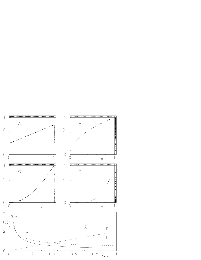
Figure 7: Examples of variable changes.

The title of this section is similar to that of Sec.  5, but the problem and the conclusions will be different. There we said that the Indifference Principle (or, in its refined modern version, the Maximum Entropy Principle) was a good choice. Here there are problems with infinities and with the fact that it is possible to map an infinite number of points contained in a finite region onto an infinite number of points contained in a larger or smaller finite region. This changes the probability density function. If, moreover, the transformation from one set of variables to the other is not linear (see, e.g. Fig.  7) what is uniform in one variable ($X$) is not uniform in another variable (e.g. $Y=X^{2}$). This problem does not exist in the case of discrete variables, since if $X=x_{i}$ has a probability $f(x_{i})$ then $Y=x_{i}^{2}$ has the same probability. A different way of stating the problem is that the Jacobian of the transformation squeezes or stretches the metrics, changing the probability density function.

We will not enter into the open discussion about the optimal choice of the distribution. Essentially we shall use the uniform distribution, being careful to employ the variable which “seems” most appropriate for the problem, but You may disagree - surely with good reason - if You have a different kind of experiment in mind.

The same problem is also present, but well hidden, in the maximum likelihood method. For example, it is possible to demonstrate that, in the case of normally distributed likelihoods, a uniform distribution of the mean $\mu$ is implicitly assumed (see section 11). There is nothing wrong with this, but one should be aware of it.

10.2 Bertrand paradox and angels’ sex

A good example to help understand the problems outlined in the previous section is the so-called Bertrand paradox:

Problem:

Given a circle of radius $R$ and a chord drawn randomly on it, what is the probability that the length $L$ of the chord is smaller than $R$?

Solution 1:

Choose “randomly” two points on the circumference and draw a chord between them: $\Rightarrow P(L<R)=1/3=0.33$ .

Solution 2:

Choose a straight line passing through the center of the circle; then draw a second line, orthogonal to the first, and which intersects it inside the circle at a “random” distance from the center: $\Rightarrow P(L<R)=1-\sqrt{3}/2=0.13$ .

Solution 3:

Choose “randomly” a point inside the circle and draw a straight line orthogonal to the radius that passes through the chosen point $\Rightarrow P(L<R)=1/4=0.25$;

Your solution:

$\ldots$ $\ldots$ $\ldots$?

Question:

What is the origin of the paradox?

Answer:

The problem does not specify how to “randomly” choose the chord. The three solutions take a uniform distribution: along the circumference; along the the radius; inside the area. What is uniform in one variable is not uniform in the others!

Question:

Which is the right solution?

In principle you may imagine an infinite number of different solutions. From a physicist’s viewpoint any attempt to answer this question is a waste of time. The reason why the paradox has been compared to the Byzantine discussions about the sex of angels is that there are indeed people arguing about it. For example, there is a school of thought which insists that Solution 2 is the right one.

In fact this kind of paradox, together with abuse of the Indifference Principle for problems like “what is the probability that the sun will rise tomorrow morning” threw a shadow over Bayesian methods at the end of last century. The maximum likelihood method, which does not make explicit use of prior distributions, was then seen as a valid solution to the problem. But in reality the ambiguity of the proper metrics on which the initial distribution is uniform has an equivalent on the arbitrariness of the variable used in the likelihood function. In the end, what was criticized when it was stated explicitly in the Bayes formula is accepted passively when it is hidden in the maximum likelihood method.

11 Normally distributed observables

11.1 Final distribution, prevision and credibility intervals of the true value

The first application of the Bayesian inference will be that of a normally distributed quantity. Let us take a data sample $\underline{q}$ of $n_{1}$ measurements, of which we calculate the average $\overline{q}_{n_{1}}$. In our formalism $\overline{q}_{n_{1}}$ is a realization of the random variable $\overline{Q}_{n_{1}}$. Let us assume we know the standard deviation $\sigma$ of the variable $Q$, either because $n_{1}$ is very large and it can be estimated accurately from the sample or because it was known a priori (we are not going to discuss in these notes the case of small samples and unknown variance). The property of the average (see  7.2) tells us that the likelihood $f(\overline{Q}_{n_{1}}|\mu,\sigma)$ is gaussian:

$$\overline{Q}_{n_{1}}\sim{\cal N}(\mu,\sigma/\sqrt{n_{1}}).$$ (116)

To simplify the following notation, let us call $x_{1}$ this average and $\sigma_{1}$ the standard deviation of the average:

$$x_{1} = \overline{q}_{n_{1}}$$ (117)

$$\sigma_{1} = \sigma/\sqrt{n_{1}}\,,$$ (118)

We then apply (108) and get

$$f(\mu|x_{1},{\cal N}(\cdot,\sigma_{1}))=\frac{\frac{1}{\sqrt{2\pi}\sigma_{1}}e^{-\frac{(x_{1}-\mu)^{2}}{2\sigma_{1}^{2}}}f_{\circ}(\mu)}{\int\frac{1}{\sqrt{2\pi}\sigma_{1}}e^{-\frac{(x_{1}-\mu)^{2}}{2\sigma_{1}^{2}}}f_{\circ}(\mu)d\mu}\,.$$ (119)

At this point we have to make a choice for $f_{\circ}(\mu)$. A reasonable choice is to take, as a first guess, a uniform distribution defined over a “large” interval which includes $x_{1}$. It is not really important how large the interval is, for a few $\sigma_{1}$’s away from $x_{1}$ the integrand at the denominator tends to zero because of the gaussian function. What is important is that a constant $f_{\circ}(\mu)$ can be simplified in (119) obtaining

$$f(\mu|x_{1},{\cal N}(\cdot,\sigma_{1}))=\frac{\frac{1}{\sqrt{2\pi}\sigma_{1}}e^{-\frac{(x_{1}-\mu)^{2}}{2\sigma_{1}^{2}}}}{\int_{-\infty}^{\infty}\frac{1}{\sqrt{2\pi}\sigma_{1}}e^{-\frac{(x_{1}-\mu)^{2}}{2\sigma_{1}^{2}}}d\mu}\,.$$ (120)

The integral in the denominator is equal to unity, since integrating with respect to $\mu_{1}$ is equivalent to integrating with respect to $x_{1}$. The final result is then

$$f(\mu)=f(\mu|x_{1},{\cal N}(\cdot,\sigma_{1}))=\frac{1}{\sqrt{2\pi}\sigma_{1}}e^{-\frac{(\mu-x_{1})^{2}}{2\sigma_{1}^{2}}}\,:$$ (121)

• the true value is normally distributed around $x_{1}$;

• its best estimate (prevision) is $E[\mu]=x_{1}$;

• its variance is $\sigma_{\mu}=\sigma_{1}$;

• the “confidence intervals”, or credibility intervals, in which there is a certain probability of finding the true value are easily calculable:

  Probability level	credibility interval
  (confidence level)	(confidence interval)
  $(\%)$
  68.3	$x_{1}$	$\pm$	$\sigma_{1}$
  90.0	$x_{1}$	$\pm$	$1.65\sigma_{1}$
  95.0	$x_{1}$	$\pm$	$1.96\sigma_{1}$
  99.0	$x_{1}$	$\pm$	$2.58\sigma_{1}$
  99.73	$x_{1}$	$\pm$	$3\sigma_{1}$

11.2 Combination of several measurements

Let us imagine making a second set of measurements of the physical quantity, which we assume unchanged from the previous set of measurements. How will our knowledge of $\mu$ change after this new information? Let us call $x_{2}=\overline{q}_{n_{2}}$ and $\sigma_{2}=\sigma^{\prime}/\sqrt{n_{2}}$ the new average and standard deviation of the average ($\sigma^{\prime}$ may be different from $\sigma$ of the sample of numerosity $n_{1}$). Applying Bayes’ theorem a second time we now have to use as initial distribution the final probability of the previous inference:

$$f(\mu|x_{1},\sigma_{1},x_{2},\sigma_{2},{\cal N})=\frac{\frac{1}{\sqrt{2\pi}\sigma_{2}}e^{-\frac{(x_{2}-\mu)^{2}}{2\sigma_{2}^{2}}}f(\mu|x_{1},{\cal N}(\cdot,\sigma_{1}))}{\int\frac{1}{\sqrt{2\pi}\sigma_{2}}e^{-\frac{(x_{2}-\mu)^{2}}{2\sigma_{2}^{2}}}f(\mu|x_{1},{\cal N}(\cdot,\sigma_{1}))d\mu}\,{}.$$ (122)

The integral is not as simple as the previous one, but still feasible analytically. The final result is

$$f(\mu|x_{1},\sigma_{1},x_{2},\sigma_{2},{\cal N})=\frac{1}{\sqrt{2\pi}\sigma_{A}}e^{-\frac{(\mu-x_{A})^{2}}{2\sigma_{A}^{2}}}\,,$$ (123)

where

$$x_{A} = \frac{x_{1}/\sigma_{1}^{2}+x_{2}/\sigma_{2}^{2}}{1/\sigma_{1}^{2}+1/\sigma_{2}^{2}}\,,$$ (124)

$$\frac{1}{\sigma_{A}^{2}} = \frac{1}{\sigma_{1}^{2}}+\frac{1}{\sigma_{2}^{2}}\,.$$ (125)

One recognizes the famous formula of the weighted average with the inverse of the variances, usually obtained from maximum likelihood. Some remarks:

• Bayes’ theorem updates the knowledge about $\mu$ in an automatic and natural way;

• if $\sigma_{1}\gg\sigma_{2}$ (and $x_{1}$ is not “too far” from $x_{2}$) the final result is only determined by the second sample of measurements. This suggests that an alternative vague a priori distribution can be, instead of the uniform, a gaussian with a large enough variance and a reasonable mean;

• the combination of the samples requires a subjective judgement that the two samples are really coming from the same true value $\mu$. We will not discuss this point in these notes, but a hint on how to proceed is: take the inference on the difference of two measurements, $D$, as explained at the end of Section  13.1 and judge yourself if $D=0$ is consistent with the probability density function of $D$.

11.3 Measurements close to the edge of the physical region

A case which has essentially no solution in the maximum likelihood approach is when a measurement is performed at the edge of the physical region and the measured value comes out very close to it, or even on the unphysical region. Let us take a numeric example:

Problem:

An experiment is planned to measure the (electron) neutrino mass. The simulations show that the mass resolution is $3.3\,\mbox{eV}/c^{2}$, largely independent of the mass value, and that the measured mass is normally distributed around the true mass. The mass value which results from the elaboration, and corrected for all known systematic effects, is $x=-5.41\,\mbox{eV}/c^{2}$. What have we learned about the neutrino mass?

Solution:

Our a priori value of the mass is that it is positive and not too large (otherwise it would already have been measured in other experiments). One can take any vague distribution which assigns a probability density function between 0 and 20 or 30 $\mbox{eV}/c^{2}$. In fact, if an experiment having a resolution of $\sigma=3.3\,\mbox{eV}/c^{2}$ has been planned and financed by rational people, with the hope of finding evidence of non negligible mass it means that the mass was thought to be in that range. If there is no reason to prefer one of the values in that interval a uniform distribution can be used, for example

$$f_{\circ K}(m)=k=1/30\hskip 28.45274pt(0\leq m\leq 30)\,.$$ (126)

Otherwise, if one thinks there is a greater chance of the mass having small rather than high values, a prior which reflects such an assumption could be chosen, for example a half normal with $\sigma_{\circ}=10\,eV$

$$f_{\circ N}(m)=\frac{2}{\sqrt{2\pi}\sigma_{\circ}}\exp{\left[-\frac{m^{2}}{2\sigma_{\circ}^{2}}\right]}\hskip 28.45274pt(m\geq 0)\,,$$ (127)

or a triangular distribution

$$f_{\circ T}(m)=\frac{1}{450}(30-x)\hskip 17.07182pt(0\leq m\leq 30)\,.$$ (128)

Let us consider for simplicity the uniform distribution

$$f(m|x,f_{\circ K}) = \frac{\frac{1}{\sqrt{2\pi}\sigma}\exp{\left[-\frac{(m-x)^{2}}{2\sigma^{2}}\right]}k}{\int_{0}^{30}\frac{1}{\sqrt{2\pi}\sigma}\exp{\left[-\frac{(m-x)^{2}}{2\sigma^{2}}\right]}kd\mu}$$ (129)

$$= \frac{19.8}{\sqrt{2\pi}\sigma}\exp{\left[-\frac{(m-x)^{2}}{2\sigma^{2}}\right]}\hskip 19.91684pt(0\leq m\leq 30)\,.$$ (130)

The value which has the highest degree of belief is $m=0$, but $f(m)$ is non vanishing up to $30\,\mbox{eV}/c^{2}$ (even if very small). We can define an interval, starting from $m=0$, in which we believe that $m$ should have a certain probability. For example this level of probability can be $95\,\%$. One has to find the value $m_{\circ}$ for which the cumulative function $F(m_{\circ})$ equals 0.95. This value of $m$ is called the upper limit (or upper bound). The result is

$$m<3.9\,\mbox{eV}/c^{2}\hskip 14.22636ptat\ 0.95\,\%\ C.L.\,.$$ (131)

If we had assumed the other initial distributions the limit would have been in both cases

$$m<3.7\,\mbox{eV}/c^{2}\hskip 14.22636ptat\ 0.95\,\%\ C.L.\,,$$ (132)

practically the same (especially if compared with the experimental resolution of $3.3\,\mbox{eV}/c^{2}$).

Comment:

Let us assume an a priori function sharply peaked at zero and see what happens. For example it could be of the kind

$$f_{\circ S}(m)\propto\frac{1}{m}\,.$$ (133)

To avoid singularities in the integral, let us take a power of $m$ a bit greater than $-1$, for example $-0.99$, and let us limit its domain to 30, getting

$$f_{\circ S}(m)=\frac{0.01\cdot 30^{0.01}}{m^{0.99}}\,.$$ (134)

The upper limit becomes

$$m<0.006\,\mbox{eV}/c^{2}\hskip 14.22636ptat\ 0.95\,\%\ C.L.\,.$$ (135)

Any experienced physicist would find this result ridiculous. The upper limit is less then $0.2\,\%$ of the experimental resolution; like expecting to resolve objects having dimensions smaller than a micron with a design ruler! Notice instead that in the previous examples the limit was always of the order of magnitude of the experimental resolution $\sigma$. As $f_{\circ S}(m)$ becomes more and more peaked at zero (power of $x\rightarrow 1$) the limit gets smaller and smaller. This means that, asymptotically, the degree of belief that $m=0$ is so high that whatever you measure you will conclude that $m=0$: you could use the measurement to calibrate the apparatus! This means that this choice of initial distribution was unreasonable.

12 Counting experiments

12.1 Binomially distributed quantities

Figure 8: Probability density function of the binomial parameter $p$, having observed $x$ successes in $n$ trials.

Let us assume we have performed $n$ trials and obtained $x$ favorable events. What is the probability of the next event? This situation happens frequently when measuring efficiencies, branching ratios, etc. Stated more generally, one tries to infer the “constant and unknown probability” of an event occurring.

Where we can assume that the probability is constant and the observed number of favorable events are binomially distributed, the unknown quantity to be measured is the parameter $p$ of the binomial. Using Bayes’ theorem we get

$$f(p|x,n,{\cal B}) = \frac{f(x|{\cal B}_{n,p})f_{\circ}(p)}{\int_{0}^{1}f(x|{\cal B}_{n,p})f_{\circ}(p)dp}$$ (136)

$$= \frac{\frac{n!}{(n-x)!x!}p^{x}(1-p)^{n-x}f_{\circ}(p)}{\int_{0}^{1}\frac{n!}{(n-x)!x!}p^{x}(1-p)^{n-x}f_{\circ}(p)dp}$$

$$= \frac{p^{x}(1-p)^{n-x}}{\int_{0}^{1}p^{x}(1-p)^{n-x}dp}\,,$$

where an initial uniform distribution has been assumed. The final distribution is known to statisticians as $\beta$ distribution since the integral at the denominator is the special function called $\beta$, defined also for real values of $x$ and $n$ (technically this is a $\beta$ with parameters $a=x+1$ and $b=n-x+1$). In our case these two numbers are integer and the integral becomes equal to $x!(n-x)!/(n+1)!$. We then get

$$f(p|x,n,{\cal B})=\frac{(n+1)!}{x!(n-x)!}p^{x}(1-p)^{n-x}\,.$$ (137)

The expected value and the variance of this distribution are:

$$E[p] = \frac{x+1}{n+2}$$ (138)

$$Var(p) = \frac{(x+1)(n-x+1)}{(n+3)(n+2)^{2}}$$

$$= \frac{x+1}{n+2}\left(\frac{n}{n+2}-\frac{x+1}{n+2}\right)\frac{1}{n+3}$$

$$= E[p]\left(\frac{n}{n+2}-E[p]\right)\frac{1}{n+3}\,.$$ (140)

The value of $p$ for which $f(p)$ has the maximum is instead $p_{m}=x/n$. The expression $E[p]$ gives the prevision of the probability for the $(n+1)$-th event occurring and is called the “recursive Laplace formula”, or “Laplace’s rule of succession”.

When $x$ and $n$ become large, and $0\ll x\ll n$, $f(p)$ has the following asymptotic properties:

$$E[p] \approx p_{m}=\frac{x}{n}\,;$$ (141)

$$Var(p) \approx \frac{x}{n}\left(1-\frac{x}{n}\right)\frac{1}{n}=\frac{p_{m}(1-p_{m})}{n}\,;$$ (142)

$$\sigma_{p} \approx \sqrt{\frac{p_{m}(1-p_{m})}{n}}:$$ (143)

$$p \sim {\cal N}(p_{m},\sigma_{p})\,.$$ (144)

Under these conditions the frequentistic “definition” of probability ($x/n$) is recovered.

Let us see two particular situations: when $x=0$ and $x=n$. In these cases one gives the result as upper or lower limits, respectively. Let us sketch the solutions:

• x=n:

  $$f(n|{\cal B}_{n,p}) = p^{n};$$ (145)

  $$f(p|x=n,{\cal B}) = \frac{p^{n}}{\int_{0}^{1}p^{n}dp}=(n+1)\cdot p^{n};$$ (146)

  $$F(p|x=n,{\cal B}) = p^{n+1}\,.$$ (147)

  To get the $95\,\%$ lower bound (limit):

  $$F(p_{\circ}|x=n,{\cal B}) = 0.05\,,$$

  $$p_{\circ} = \sqrt[n+1]{0.05}\,.$$ (148)

  An increasing number of trials $n$ constrain more and more $p$ around 1.

• x=0:

  $$f(0|{\cal B}_{n,p}) = (1-p)^{n};$$ (149)

  $$f(p|x=0,n,{\cal B}) = \frac{(1-p)^{n}}{\int_{0}^{1}(1-p)^{n}dp}=(n+1)\cdot(1-p)^{n};$$ (150)

  $$F(p|x=0,n,{\cal B}) = 1-(1-p)^{n+1}\,.$$ (151)

  To get the $95\,\%$ upper bound (limit):

  $$F(p_{\circ}|x=0,n,{\cal B}) = 0.95;$$

  $$p_{\circ} = 1-\sqrt[n+1]{0.05}\,.$$ (152)

The following table shows the $95\,\%$ C.L. limits as a function of $n$. The Poisson approximation, to be discussed in the next section, is also shown.

	Probability level = $95\,\%$
$n$	$x=n$	$x=0$
	binomial	binomial	Poisson approx.
			( $p_{\circ}=3/n$ )
3	$p\geq 0.47$	$p\leq 0.53$	$p\leq 1$
5	$p\geq 0.61$	$p\leq 0.39$	$p\leq 0.6$
10	$p\geq 0.76$	$p\leq 0.24$	$p\leq 0.3$
50	$p\geq 0.94$	$p\leq 0.057$	$p\leq 0.06$
100	$p\geq 0.97$	$p\leq 0.029$	$p\leq 0.03$
1000	$p\geq 0.997$	$p\leq 0.003$	$p\leq 0.003$

To show in this simple case how $f(p)$ is updated by the new information, let us imagine we have performed two experiments. The results are $x_{1}=n_{1}$ and $x_{2}=n_{2}$, respectively. Obviously the global information is equivalent to $x=x_{1}+x_{2}$ and $n=n_{1}+n_{2}$, with $x=n$. We then get

$$f(p|x=n,{\cal B})=(n+1)p^{n}=(n_{1}+n_{2}+1)p^{n_{1}+n_{2}}\,.$$ (153)

A different way of proceeding would have been to calculate the final distribution from the information $x_{1}=n_{1}$

$$f(p|x_{1}=n_{1},{\cal B})=(n_{1}+1)p^{n_{1}}\,,$$ (154)

and feed it as initial distribution to the next inference:

$$f(p|x_{1}=n_{1},x_{2}=n_{2},{\cal B}) = \frac{p^{n_{2}}f(p|x_{1}=n_{1},{\cal B})}{\int_{0}^{1}p^{n_{2}}f(p|x_{1}=n_{1},{\cal B})dp}$$ (155)

$$= \frac{p^{n_{2}}(n_{1}+1)p^{n_{1}}}{\int_{0}^{1}p^{n_{2}}(n_{1}+1)p^{n_{1}}dp}$$ (156)

$$= (n_{1}+n_{2}+1)p^{n_{1}+n_{2}}\,,$$ (157)

getting the same result.

12.2 Poisson distributed quantities

As is well known, the typical application of the Poisson distribution is in counting experiments such as source activity, cross sections, etc. The unknown parameter to be inferred is $\lambda$. Applying Bayes formula we get

$$f(\lambda|x,{\cal P}) = \frac{\frac{\lambda^{x}e^{-\lambda}}{x!}f_{\circ}(\lambda)}{\int_{0}^{\infty}\frac{\lambda^{x}e^{-\lambda}}{x!}f_{\circ}(\lambda)d\lambda}\,.$$ (158)

Assuming $f_{\circ}(\lambda)$ constant up to a certain $\lambda_{max}\gg x$ and making the integral by parts we obtain

$$f(\lambda|x,{\cal P}) = \frac{\lambda^{x}e^{-\lambda}}{x!}$$ (159)

$$F(\lambda|x,{\cal P}) = 1-e^{-\lambda}\left(\sum_{n=0}^{x}\frac{\lambda^{n}}{n!}\right)\,,$$ (160)

where the last result has been obtained integrating (159) also by parts. Fig.  9 shows how to build the credibility intervals, given a certain measured number of counts $x$.

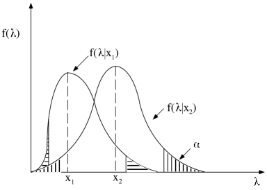
Figure 9: Poisson parameter $\lambda$ inferred from an observed number $x$ of counts.

Fig.  10 shows some numerical examples.

Figure 10: Examples of $f(\lambda|x_{i})$.

$f(\lambda)$ has the following properties:

• the expected values, variance, value of maximum probability are

  $$E[\lambda] = x+1$$ (161)

  $$Var(\lambda) = x+2$$ (162)

  $$\lambda_{m} = x\,;$$ (163)

  the fact that the best estimate of $\lambda$ in the Bayesian sense is not the intuitive value $x$ but $x+1$ should neither surprise, nor disappoint us: according to the initial distribution used “there are always more possible values of $\lambda$ on the right side than on the left side of $x$”, and they pull the distribution to their side; the full information is always given by $f(\lambda)$ and the use of the mean is just a rough approximation; the difference from the “desired” intuitive value $x$ in units of the standard deviation goes as $1/\sqrt{n+2}$ and becomes immediately negligible;

• when $x$ becomes large we get:

  $$E[\lambda] \approx \lambda_{m}=x\,;$$ (164)

  $$Var(\lambda) \approx \lambda_{m}=x\,;$$ (165)

  $$\sigma_{\lambda} \approx \sqrt{x}\,;$$ (166)

  $$\lambda \sim {\cal N}(x,\sqrt{x})\,.$$ (167)

  (166) is one of the most familar formulae used by physicists to assess the uncertainty of a measurement, although it is sometimes misused.

Let us conclude with a special case: $x=0$. As one might imagine, the inference is highly sensitive to the initial distribution. Let us assume that the experiment was planned with the hope of observing something, i.e. that it could detect a handful of events within its lifetime. With this hypothesis one may use any vague prior function not strongly peaked at zero. We have already come across a similar case in section  11.3, concerning the upper limit of the neutrino mass. There it was shown that reasonable hypotheses based on the positive attitude of the experimentalist are almost equivalent and that they give results consistent with detector performances. Let us use then the uniform distribution

$$f(\lambda|x=0,{\cal P}) = e^{-\lambda}$$ (168)

$$F(\lambda|x=0,{\cal P}) = 1-e^{-\lambda}$$ (169)

$$\lambda < 3\ at\ 95\,\%\ C.L.\,.$$ (170)

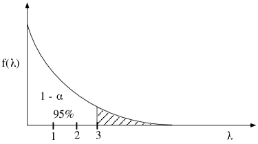
Figure 11: Upper limit to $\lambda$ having observed 0 events.

13 Uncertainty due to unknown systematic errors

13.1 Example: uncertainty of the instrument scale offset

In our scheme any quantity of influence of which we don’t know the exact value is a source of systematic error. It will change the final distribution of $\mu$ and hence its uncertainty. We have already discussed the most general case in  9.1. Let us make a simple application making a small variation to the example in section  11.1: the “zero” of the instrument is not known exactly, owing to calibration uncertainty. This can be parametrized assuming that its true value $Z$ is normally distributed around 0 (i.e. the calibration was properly done!) with a standard deviation $\sigma_{Z}$. Since, most probably, the true value of $\mu$ is independent from the true value of $Z$, the initial joint probability density function can be written as the product of the marginal ones:

$$f_{\circ}(\mu,z)=f_{\circ}(\mu)f_{\circ}(z)=k\frac{1}{\sqrt{2\pi}\sigma_{Z}}\exp{\left[-\frac{z^{2}}{2\sigma_{Z}^{2}}\right]}\,.$$ (171)

Also the likelihood changes with respect to  116:

$$f(x_{1}|\mu,z)=\frac{1}{\sqrt{2\pi}\sigma_{1}}\exp{\left[-\frac{(x_{1}-\mu-z)^{2}}{2\sigma_{1}^{2}}\right]}\,.$$ (172)

Putting all the pieces together and making use of (107) we finally get

$$f(\mu|x_{1},\ldots,f_{\circ}(z))=\frac{\int\frac{1}{\sqrt{2\pi}\sigma_{1}}\exp{\left[-\frac{(x_{1}-\mu-z)^{2}}{2\sigma_{1}^{2}}\right]}\frac{1}{\sqrt{2\pi}\sigma_{Z}}\exp{\left[-\frac{z^{2}}{2\sigma_{Z}^{2}}\right]}dz}{\int\!\!\int\frac{1}{\sqrt{2\pi}\sigma_{1}}\exp{\left[-\frac{(x_{1}-\mu-z)^{2}}{2\sigma_{1}^{2}}\right]}\frac{1}{\sqrt{2\pi}\sigma_{Z}}\exp{\left[-\frac{z^{2}}{2\sigma_{Z}^{2}}\right]}d\mu dz}\,.$$

Integrating we get

$$f(\mu)=f(\mu|x_{1},\ldots,f_{\circ}(z))=\frac{1}{\sqrt{2\pi}\sqrt{\sigma_{1}^{2}+\sigma_{Z}^{2}}}\exp{\left[-\frac{(\mu-x_{1})^{2}}{2(\sigma_{1}^{2}+\sigma_{Z}^{2})}\right]}\,.$$ (173)

The result is that $f(\mu)$ is still a gaussian, but with a larger variance. The global standard uncertainty is the quadratic combination of that due to the statistical fluctuation of the data sample and the uncertainty due to the imperfect knowledge of the systematic effect:

$$\sigma_{tot}^{2}=\sigma_{1}^{2}+\sigma_{Z}^{2}\,.$$ (174)

This result is well known, although there are still some “old-fashioned” recipes which require different combinations of the contributions to be performed.

One has to notice that in this framework it makes no sense to speak of “statistical” and “systematical” uncertainties, as if they were of a different nature. They have the same probabilistic nature: $\overline{Q}_{n_{1}}$ is around $\mu$ with a standard deviation $\sigma_{1}$, and $Z$ is around 0 with standard deviation $\sigma_{Z}$. What distinguishes the two components is how the knowledge of the uncertainty is gained: in one case ($\sigma_{1}$) from repeated measurements; in the second case ($\sigma_{Z}$) the evaluation was done by somebody else (the constructor of the instrument), or in a previous experiment, or guessed from the knowledge of the detector, or by simulation, etc. This is the reason why the ISO Guide [2] prefers the generic names Type A and Type B for the two kinds of contribution to global uncertainty. In particular the name “systematic uncertainty” should be avoided, while it is correct to speak about “uncertainty due to a systematic effect”.

13.2 Correction for known systematic errors

It is easy to be convinced that if our prior knowledge about $Z$ was of the kind

$$Z\sim{\cal N}(z_{\circ},\sigma_{Z})$$ (175)

the result would have been

$$\mu\sim{\cal N}\left(x_{1}-z_{\circ},\sqrt{\sigma_{1}^{2}+\sigma_{Z}^{2}}\right)\,,$$ (176)

i.e. one has first to correct the result for the best value of the systematic error and then include in the global uncertainty a term due to imperfect knowledge about it. This is a well known and practised procedure, although there are still people who confuse $z_{\circ}$ with its uncertainty.

13.3 Measuring two quantities with the same instrument having an uncertainty of the scale offset

Let us take an example which is a bit more complicated (at least from the mathematical point of view) but conceptually very simple and also very common in laboratory practice. We measure two physical quantities with the same instrument, assumed to have an uncertainty on the “zero”, modeled with a normal distribution as in the previous sections. For each of the quantities we collect a sample of data under the same conditions, which means that the unknown offset error does not change from one set of measurements to the other. Calling $\mu_{1}$ and $\mu_{2}$ the true values, $x_{1}$ and $x_{2}$ the sample averages, $\sigma_{1}$ and $\sigma_{2}$ the average’s standard deviations, and $Z$ the true value of the “zero”, the initial probability density and the likelihood are

$$f_{\circ}(\mu_{1},\mu_{2},z)=f_{\circ}(\mu_{1})f_{\circ}(\mu_{2})f_{\circ}(z)=k\frac{1}{\sqrt{2\pi}\sigma_{Z}}\exp{\left[-\frac{z^{2}}{2\sigma_{Z}^{2}}\right]}$$ (177)

and

$$f(x_{1},x_{2}|\mu_{1},\mu_{2},z) = \frac{1}{\sqrt{2\pi}\sigma_{1}}\exp{\left[-\frac{(x_{1}-\mu_{1}-z)^{2}}{2\sigma_{1}^{2}}\right]}\frac{1}{\sqrt{2\pi}\sigma_{2}}\exp{\left[-\frac{(x_{2}-\mu_{2}-z)^{2}}{2\sigma_{2}^{2}}\right]}$$ (178)

$$= \frac{1}{2\pi\sigma_{1}\sigma_{2}}\exp{\left[-\frac{1}{2}\left(\frac{(x_{1}-\mu_{1}-z)^{2}}{\sigma_{1}^{2}}+\frac{(x_{2}-\mu_{2}-z)^{2}}{\sigma_{2}^{2}}\right)\right]}\,,$$

respectively. The result of the inference is now the joint probability density function of $\mu_{1}$ and $\mu_{2}$:

$$f(\mu_{1},\mu_{2}|x_{1},x_{2},\sigma_{1},\sigma_{2},f_{\circ}(z)) = \frac{\int f(x_{1},x_{2}|\mu_{1},\mu_{2},z)f_{\circ}(\mu_{1},\mu_{2},z)dz}{\int\!\!\int\!\!\int f(x_{1},x_{2}|\mu_{1},\mu_{2},z)f_{\circ}(\mu_{1},\mu_{2},z)d\mu_{1}d\mu_{2}dz}\,,\$$ (179)

where expansion of the functions has been omitted for the sake of clarity. Integrating we get

$$f(\mu_{1},\mu_{2}) = \frac{1}{2\pi\sqrt{\sigma_{1}^{2}+\sigma_{Z}^{2}}\sqrt{\sigma_{2}^{2}+\sigma_{Z}^{2}}\sqrt{1-\rho^{2}}}$$

$$\exp{\left\{-\frac{1}{2(1-\rho^{2})}\left[\frac{(\mu_{1}-x_{1})^{2}}{\sigma_{1}^{2}+\sigma_{Z}^{2}}-2\rho\frac{(\mu_{1}-x_{1})(\mu_{2}-x_{2})}{\sqrt{\sigma_{1}^{2}+\sigma_{Z}^{2}}\sqrt{\sigma_{2}^{2}+\sigma_{Z}^{2}}}+\frac{(\mu_{2}-x_{2})^{2}}{\sigma_{2}^{2}+\sigma_{Z}^{2}}\right]\right\}}\,.$$

where

$$\rho=\frac{\sigma_{Z}^{2}}{\sqrt{\sigma_{1}^{2}+\sigma_{Z}^{2}}\sqrt{\sigma_{2}^{2}+\sigma_{Z}^{2}}}\,.$$ (181)

If $\sigma_{Z}$ vanishes then (13.3) has the simpler expression

$$f(\mu_{1},\mu_{2})@>>{\sigma_{Z}\rightarrow 0}>\frac{1}{\sqrt{2\pi}\sigma_{1}}\exp{\left[-\frac{(\mu_{1}-x_{1})^{2}}{2\sigma_{1}^{2}}\right]}\frac{1}{\sqrt{2\pi}\sigma_{2}}\exp{\left[-\frac{(\mu_{2}-x_{2})^{2}}{2\sigma_{2}^{2}}\right]}\,,$$ (182)

i.e. if there is no uncertainty on the offset calibration the joint density function then $f(\mu_{1},\mu_{2})$ is equal to the product of two independent normal functions, i.e. $\mu_{1}$ and $\mu_{2}$ are independent. In the general case we have to conclude that:

• the effect of the common uncertainty $\sigma_{Z}$ makes the two values correlated, since they are affected by a common unknown systematic error; the correlation coefficient is always non negative ($\rho\geq 0$), as intuitively expected from the definition of systematic error;

• the joint density function is a multinormal distribution of parameters $x_{1}$, $\sigma_{\mu_{1}}=\sqrt{\sigma_{1}^{2}+\sigma_{Z}^{2}}$, $x_{2}$, $\sigma_{\mu_{2}}=\sqrt{\sigma_{2}^{2}+\sigma_{Z}^{2}}$, and $\rho$ (see example of Fig.  5);

• the marginal distributions are still normal:

  $$\mu_{1} \sim {\cal N}\left(x_{1},\sqrt{\sigma_{1}^{2}+\sigma_{Z}^{2}}\right)$$ (183)

  $$\mu_{2} \sim {\cal N}\left(x_{2},\sqrt{\sigma_{2}^{2}+\sigma_{Z}^{2}}\right)\,;$$ (184)

• the covariance between $\mu_{1}$ and $\mu_{2}$ is

  $$Cov(\mu_{1},\mu_{2}) = \rho\sigma_{\mu_{1}}\sigma_{\mu_{2}}$$ (185)

  $$= \rho\sqrt{\sigma_{1}^{2}+\sigma_{Z}^{2}}\sqrt{\sigma_{2}^{2}+\sigma_{Z}^{2}}=\sigma_{Z}^{2}\,.$$

• the distribution of any function $g(\mu_{1},\mu_{2})$ can be calculated using the standard methods of probability theory. For example, one can demonstrate that the sum $S=\mu_{1}+\mu_{2}$ and the difference $D=\mu_{1}-\mu_{2}$ are also normally distributed (see also the introductory discussion to the central limit theorem and section  16 for the calculation of averages and standard deviations):

  $$S \sim {\cal N}\left(x_{1}+x_{2},\sqrt{\sigma_{1}^{2}+\sigma_{2}^{2}+(2\sigma_{Z})^{2}}\right)$$ (186)

  $$D \sim {\cal N}\left(x_{1}-x_{2},\sqrt{\sigma_{1}^{2}+\sigma_{2}^{2}}\right)\,.$$ (187)

  The result can be interpreted in the following way:

  • the uncertainty on the difference does not depend on the common offset uncertainty: whatever the value of the true “zero” is, it cancels in differences;

  • in the sum, instead, the effect of the common uncertainty is somewhat amplified since it enters “in phase” in the global uncertainty of each of the quantities.

13.4 Indirect calibration

Let us use the result of the previous section to solve another typical problem of measurements. Suppose that after (or before, it doesn’t matter) we have done the measurements of $x_{1}$ and $x_{2}$ and we have the final result, summarized in (13.3), we know the “exact” value of $\mu_{1}$ (for example we perform the measurement on a reference). Let us call it $\mu_{1}^{\circ}$. Will this information provide a better knowledge of $\mu_{2}$? In principle yes: the difference between $x_{1}$ and $\mu_{1}^{\circ}$ defines the systematic error (the true value of the “zero” $Z$). This error can then be subtracted from $\mu_{2}$ to get a corrected value. Also the overall uncertainty of $\mu_{2}$ should change, intuitively it “should” decrease, since we are adding new information. But its value doesn’t seem to be obvious, since the logical link between $\mu_{1}^{\circ}$ and $\mu_{2}$ is $\mu_{1}^{\circ}\rightarrow Z\rightarrow\mu_{2}$.

The problem can be solved exactly using the concept of conditional probability density function $f(\mu_{2}|\mu_{1}^{\circ})$ (see (95-96)). We get

$$\Large{\mu_{2|\mu_{1}^{\circ}}\sim}{\Large\cal N}\left(x_{2}+\frac{\sigma_{Z}^{2}}{\sigma_{1}^{2}+\sigma_{Z}^{2}}(\mu_{1}^{\circ}-x_{1}),\ \sqrt{\sigma_{2}^{2}+\left(\frac{1}{\sigma_{1}^{2}}+\frac{1}{\sigma_{Z}^{2}}\right)^{-1}}\right)\,.$$ (188)

The best value of $\mu_{2}$ is shifted by an amount $\Delta$, with respect to the measured value $x_{2}$, which is not exactly $x_{1}-\mu_{1}^{\circ}$, as was naïvely guessed, and the uncertainty depends on $\sigma_{2}$, $\sigma_{Z}$ and $\sigma_{1}$. It is easy to be convinced that the exact result is more resonable than the (suggested) first guess. Let us rewrite $\Delta$ in two different ways:

$$\Delta = \frac{\sigma_{Z}^{2}}{\sigma_{1}^{2}+\sigma_{Z}^{2}}(\mu_{1}^{\circ}-x_{1})$$ (189)

$$= \frac{1}{\frac{1}{\sigma_{1}^{2}}+\frac{1}{\sigma_{Z}^{2}}}\left[\frac{1}{\sigma_{1}^{2}}\cdot(x_{1}-\mu_{1}^{\circ})+\frac{1}{\sigma_{Z}^{2}}\cdot 0\right]\,.$$ (190)

• Eq. (189) shows that one has to apply the correction $x_{1}-\mu_{1}^{\circ}$ only if $\sigma_{1}=0$. If instead $\sigma_{Z}=0$ there is no correction to be applied, since the instrument is perfectly calibrated. If $\sigma_{1}\approx\sigma_{Z}$ the correction is half of the measured difference between $x_{1}$ and $\mu_{1}^{\circ}$;

• Eq. (190) shows explicitly what is going on and why the result is consistent with the way we have modeled the uncertainties. In fact we have performed two independent calibrations: one of the offset and one of $\mu_{1}$. The best estimate of the true value of the “zero” $Z$ is the weighted average of the two measured offsets;

• the new uncertainty of $\mu_{2}$ (see (188)) is a combination of $\sigma_{2}$ and the uncertainty of the weighted average of the two offsets. Its value is smaller than what one would have with only one calibration and, obviously, larger than that due to the sampling fluctuations alone:

  $$\sigma_{2}\leq\sqrt{\sigma_{2}^{2}+\frac{\sigma_{1}^{2}\sigma_{Z}^{2}}{\sigma_{1}^{2}+\sigma_{Z}^{2}}}\leq\sqrt{\sigma_{2}^{2}+\sigma_{Z}^{2}}\,.$$ (191)

13.5 Counting measurements in presence of background

As an example of a different kind of systematic effect, let us think of counting experiments in the presence of background. For example we are searching for a new particle, we make some selection cuts and count $x$ events. But we also expect an average number of background events $\lambda_{B_{\circ}}\pm\sigma_{B}$, where $\sigma_{B}$ is the standard uncertainty of $\lambda_{B_{\circ}}$, not to be confused with $\sqrt{\lambda_{B_{\circ}}}$. What can we say about $\lambda_{S}$, the true value of the average number associated to the signal? First we will treat the case on which the determination of the expected number of background events is well known ($\sigma_{B}/\lambda_{B_{\circ}}\ll 1$), and then the general case:

$\sigma_{B}/\lambda_{B_{\circ}}\ll 1$:

the true value of the sum of signal and background is $\lambda=\lambda_{S}+\lambda_{B_{\circ}}$. The likelihood is

$$P(x|\lambda)=\frac{e^{-\lambda}\lambda^{x}}{x!}\,.$$ (192)

Applying Bayes’s theorem we have

$$f(\lambda_{S}|x,\lambda_{B_{\circ}}) = \frac{e^{-(\lambda_{B_{\circ}}+\lambda_{S})}(\lambda_{B_{\circ}}+\lambda_{S})^{x}f_{\circ}(\lambda_{S})}{\int_{0}^{\infty}e^{-(\lambda_{B_{\circ}}+\lambda_{S})}(\lambda_{B_{\circ}}+\lambda_{S})^{x}f_{\circ}(\lambda_{S})d\lambda_{S}}\,.$$ (193)

Choosing again $f_{\circ}(\lambda_{S})$ uniform (in a reasonable interval) this gets simplified. The integral at the denominator can be done easily by parts and the final result is:

$$f(\lambda_{S}|x,\lambda_{B_{\circ}}) = \frac{e^{-\lambda_{S}}(\lambda_{B_{\circ}}+\lambda_{S})^{x}}{x!\sum_{n=0}^{x}\frac{\lambda_{B_{\circ}}^{n}}{n!}}$$ (194)

$$F(\lambda_{S}|x,\lambda_{B_{\circ}}) = 1-\frac{e^{-\lambda_{S}}\sum_{n=0}^{x}\frac{(\lambda_{B_{\circ}}+\lambda_{S})^{n}}{n!}}{\sum_{n=0}^{x}\frac{\lambda_{B_{\circ}}^{n}}{n!}}\,.$$ (195)

From (194-195) it is possible to calculate in the usual way the best estimate and the credibility intervals of $\lambda_{S}$. Two particular cases are of interest:

• if $\lambda_{B_{\circ}}=0$ then formulae (​159-​160) are recovered. In such a case one measured count is enough to claim for a signal (if somebody is willing to believe that really $\lambda_{B_{\circ}}=0$ without any uncertainty$\ldots$);

• if $x=0$ then

  $$f(\lambda|x,\lambda_{B_{\circ}})=e^{-\lambda_{S}}\,,$$ (196)

  independently of $\lambda_{B_{\circ}}$. This result is not really obvious.

Any $g(\lambda_{B_{\circ}})$:

In the general case, the true value of the average number of background events $\lambda_{B}$ is unknown. We only known that it is distributed around $\lambda_{B_{\circ}}$ with standard deviation $\sigma_{B}$ and probability density function $g(\lambda_{B})$, not necessarily a gaussian. What changes with respect to the previous case is the initial distribution, now a joint function of $\lambda_{S}$ and of $\lambda_{B}$. Assuming $\lambda_{B}$ and $\lambda_{S}$ independent the prior density function is

$$f_{\circ}(\lambda_{S},\lambda_{B})=f_{\circ}(\lambda_{S})g_{\circ}(\lambda_{B})\,.$$ (197)

We leave $f_{\circ}$ in the form of a joint distribution to indicate that the result we shall get is the most general for this kind of problem. The likelihood, on the other hand, remains the same as in the previous example. The inference of $\lambda_{S}$ is done in the usual way, applying Bayes’ theorem and marginalizing with respect to $\lambda_{S}$:

$$f(\lambda_{S}|x,g_{\circ}(\lambda_{B}))=\frac{\int e^{-(\lambda_{B}+\lambda_{S})}(\lambda_{B}+\lambda_{S})^{x}f_{\circ}(\lambda_{S},\lambda_{B})d\lambda_{B}}{\int\!\!\int e^{-(\lambda_{B}+\lambda_{S})}(\lambda_{B}+\lambda_{S})^{x}f_{\circ}(\lambda_{S},\lambda_{B})d\lambda_{S}d\lambda_{B}}\,.$$ (198)

The previous case (formula (194)) is recovered if the only value allowed for $\lambda_{B}$ is $\lambda_{B_{\circ}}$ and $f_{\circ}(\lambda_{S})$ is uniform:

$$f_{\circ}(\lambda_{S},\lambda_{B})=k\delta(\lambda_{B}-\lambda_{B_{\circ}})\,.$$ (199)

14 Approximate methods

14.1 Linearization

We have seen in the above examples how to use the general formula (107) for practical applications. Unfortunately, when the problem becomes more complicated one starts facing integration problems. For this reason approximate methods are generally used. We will derive the approximation rules consistently with the approach followed in these notes and then the resulting formulae will be compared with the ISO recommendations. To do this, let us neglect for a while all quantities of influence which could produce unknown systematic errors. In this case (107) can be replaced by (108), which can be further simplified if we remember that correlations between the results are originated by unknown systematic errors. In absence of these, the joint distribution of all quantities $\underline{\mu}$ is simply the product of marginal ones:

$$f_{R_{i}}(\underline{\mu_{i}})=\prod_{i}f_{R_{i}}(\mu_{i})\,,$$ (200)

with

$$f_{R_{i}}(\mu_{i})=f_{R_{i}}(\mu_{i}|x_{i},\underline{h}_{\circ})=\frac{f(x_{i}|\mu_{i},\underline{h}_{\circ})f_{\circ}(\mu_{i})}{\int f(x_{i}|\mu_{i},\underline{h}_{\circ})f_{\circ}(\mu_{i})d\mu_{i}}\,.$$ (201)

The symbol $f_{R_{i}}(\mu_{i})$ indicates that we are dealing with raw values evaluated at $\underline{h}=\underline{h}_{\circ}$. Since for any variation of $\underline{h}$ the inferred values of $\mu_{i}$ will change, it is convenient, to name with the same subscript $R$ the quantity obtained for $\underline{h}_{\circ}$:

$$f_{R_{i}}(\mu_{i})\longrightarrow f_{R_{i}}(\mu_{R_{i}})\,.$$ (202)

Let us indicate with $\widehat{\mu}_{R_{i}}$ and $\sigma_{R_{i}}$ the best estimates and the standard uncertainty of the raw values:

$$\widehat{\mu}_{R_{i}} = E[\mu_{R_{i}}]$$ (203)

$$\sigma_{R_{i}}^{2} = Var(\mu_{R_{i}})\,.$$ (204)

For any possible configuration of conditioning hypotheses $\underline{h}$, corrected values $\mu_{i}$ are obtained:

$$\mu_{i}=\mu_{R_{i}}+g_{i}(\underline{h})\,.$$ (205)

The function which relates the corrected value to the raw value and to the systematic effects has been denoted by $g_{i}$ not to be confused with a probability density function. Expanding (205) in series around $\underline{h}_{\circ}$ we finally arrive at the expression which will allow us to make the approximated evaluations of uncertainties:

$$\boxed{\mu_{i}=\mu_{R_{i}}+\sum_{l}\frac{\partial g_{i}}{\partial h_{l}}(h_{l}-h_{\circ_{l}})+\ldots\,}$$ (206)

(All derivatives are evaluated at $\{\widehat{\mu}_{R_{i}},\underline{h}_{\circ}\}$. To simplify the notation a similar convention will be used in the following formulae).

Neglecting the terms of the expansion above the first order, and taking the expected values, we get

$$\widehat{\mu}_{i} = E[\mu_{i}]$$ (207)

$$\approx \widehat{\mu}_{R_{i}}\,;$$

$$\sigma_{\mu_{i}}^{2} = E\left[(\mu_{i}-E[\mu_{i}])^{2}\right]$$ (208)

$$\approx \sigma_{R_{i}}^{2}+\sum_{l}\left(\frac{\partial g_{i}}{\partial h_{l}}\right)^{2}\!\sigma_{h_{l}}^{2}$$

$$\left\{+2\sum_{l<m}\left(\frac{\partial g_{i}}{\partial h_{l}}\right)\left(\frac{\partial g_{i}}{\partial h_{m}}\right)\rho_{lm}\sigma_{h_{l}}\sigma_{h_{m}}\right\}\,;$$

$$Cov(\mu_{i},\mu_{j}) = E\left[(\mu_{i}-E[\mu_{i}])(\mu_{j}-E[\mu_{j}])\right]$$ (209)

$$\approx \sum_{l}\left(\frac{\partial g_{i}}{\partial h_{l}}\right)\left(\frac{\partial g_{j}}{\partial h_{l}}\right)\sigma_{h_{l}}^{2}$$

$$\left\{+2\sum_{l<m}\left(\frac{\partial g_{i}}{\partial h_{l}}\right)\left(\frac{\partial g_{j}}{\partial h_{m}}\right)\rho_{lm}\sigma_{h_{l}}\sigma_{h_{m}}\right\}\,.$$

The terms included within $\{\cdot\}$ vanish if the unknown systematic errors are uncorrelated, and the formulae become simpler. Unfortunately, very often this is not the case, as when several calibration constants are simultaneously obtained from a fit (for example, in most linear fits slop and intercept have a correlation coefficient close to $-0.9$).

Sometimes the expansion (206) is not performed around the best values of $\underline{h}$ but around their nominal values, in the sense that the correction for the known value of the systematic errors has not yet been applied (see section 13.2). In this case (206) should be replaced by

$$\mu_{i}=\mu_{R_{i}}+\sum_{l}\frac{\partial g_{i}}{\partial h_{l}}(h_{l}-h_{N_{l}})+\ldots\,$$ (210)

where the subscript $N$ stands for nominal. The best value of $\mu_{i}$ is then

$$\widehat{\mu}_{i} = E[\mu_{i}]$$ (211)

$$\approx \widehat{\mu}_{R_{i}}+E\left[\sum_{l}\frac{\partial g_{i}}{\partial h_{l}}(h_{l}-h_{N_{l}})\right]$$

$$= \widehat{\mu}_{R_{i}}+\sum_{l}\delta\mu_{i_{l}}\,.$$

(208) and (209) instead remain valid, with the condition that the derivative is calculated at $\underline{h}_{N}$. If $\rho_{lm}=0$ it is possible to rewrite (208) and (209) in the following way, which is very convenient for practical applications:

$$\sigma_{\mu_{i}}^{2} \approx \sigma_{R_{i}}^{2}+\sum_{l}\left(\frac{\partial g_{i}}{\partial h_{l}}\right)^{2}\!\sigma_{h_{l}}^{2}$$ (212)

$$= \sigma_{R_{i}}^{2}+\sum_{l}u_{i_{l}}^{2}\,;$$ (213)

$$Cov(\mu_{i},\mu_{j}) \approx \sum_{l}\left(\frac{\partial g_{i}}{\partial h_{l}}\right)\left(\frac{\partial g_{j}}{\partial h_{l}}\right)\sigma_{h_{l}}^{2}$$ (214)

$$= \sum_{l}s_{ij_{l}}\left|\frac{\partial g_{i}}{\partial h_{l}}\right|\sigma_{h_{l}}\left|\frac{\partial g_{j}}{\partial h_{l}}\right|\sigma_{h_{l}}$$ (215)

$$= \sum_{l}s_{ij_{l}}u_{i_{l}}u_{j_{l}}$$ (216)

$$= \sum_{l}Cov_{l}(\mu_{i},\mu_{j})\,.$$ (217)

$u_{i_{l}}$ is the component to the standard uncertainty due to effect $h_{l}$. $s_{ij_{l}}$ is equal to the product of signs of the derivatives, which takes into account whether the uncertainties are positively or negatively correlated.

To summarize, when systematic effects are not correlated with each other, the following quantities are needed to evaluate the corrected result, the combined uncertainties and the correlations:

• the raw $\widehat{\mu}_{R_{i}}$ and $\sigma_{R_{i}}$;

• the best estimates of the corrections $\delta\mu_{i_{l}}$ for each systematic effect $h_{l}$;

• the best estimate of the standard deviation $u_{i_{l}}$ due to the imperfect knowledge of the systematic effect;

• for any pair $\{\mu_{i},\mu_{j}\}$ the sign of the correlation $s_{ij_{l}}$ due to the effect $h_{l}$.

In High Energy Physics applications it is frequently the case that the derivatives appearing in (211-215) cannot be calculated directly, as for example when $h_{l}$ are parameters of a simulation program, or acceptance cuts. Then variations of $\underline{\mu}_{i}$ are usually studied varying a particular $h_{l}$ within a reasonable interval, holding the other influence quantities at the nominal value. $\delta\mu_{i_{l}}$ and $u_{i_{l}}$ are calculated from the interval $\pm\Delta_{i}^{\pm}$ of variation of the true value for a given variation $\pm\Delta_{h_{l}}^{\pm}$ of $h_{l}$ and from the probabilistic meaning of the intervals (i.e. from the assumed distribution of the true value). This empirical procedure for determining $\delta\mu_{i_{l}}$ and $u_{i_{l}}$ has the advantage that it can take into account non linear effects, since it directly measures the difference $\widehat{\mu}_{i}-\widehat{\mu}_{R_{i}}$ for a given difference $h_{l}-h_{N_{l}}$.

Some examples are given in section 14.4, and two typical experimental applications will be discussed in more detail in section 16.

14.2 BIPM and ISO recommendations

In this section we compare the results obtained in the previous section with the recommendations of the Bureau International des Poids et Mésures (BIPM) and the International Organization for Standardization (ISO) on “the expression of experimental uncertainty”.

1. The uncertainty in the result of a measurement generally consists of several components which may be grouped into two categories according to the way in which their numerical value is estimated:

   A:

   those which are evaluated by statistical methods;

   B:

   those which are evaluated by other means.

   There is not always a simple correspondence between the classification into categories A or B and the previously used classification into “random” and “systematic” uncertainties. The term “systematic uncertainty” can be misleading and should be avoided.

   The detailed report of the uncertainty should consist of a complete list of the components, specifying for each the method used to obtain its numerical result.

   Essentially the first recommendation states that all uncertainties can be treated probabilistically. The distinction between types A and B is subtle and can be misleading if one thinks of “statistical methods” as synonymous with “probabilistic methods” - as currently done in High Energy Physics. Here “statistical” has the classical meaning of repeated measurements.

2. The components in category A are characterized by the estimated variances $s_{i}^{2}$ (or the estimated “standard deviations” $s_{i}$) and the number of degrees of freedom $\nu_{i}$. Where appropriate, the covariances should be given.

   The estimated variances correspond to $\sigma_{R_{i}}^{2}$ of the previous section. The degrees of freedom have are related to small samples and to the Student t distribution. The problem of small samples is not discussed in these notes, but clearly this recommendation is a relic of frequentistic methods. With the approach followed in theses notes there is no need to talk about degrees of freedom, since the Bayesian inference defines the final probability function $f(\mu)$ completely.

3. The components in category B should be characterized by quantities $u_{j}^{2}$, which may be considered as approximations to the corresponding variances, the existence of which is assumed. The quantities $u_{j}^{2}$ may the treated like variances and the quantities $u_{j}$ like standard deviations. Where appropriate, the covariances should be treated in a similar way.

   Clearly, this recommendation is meaningful only in a Bayesian framework.

4. The combined uncertainty should be characterized by the numerical value obtained by applying the usual method for the combination of variances. The combined uncertainty and its components should be expressed in the form of “standard deviations”.

   This is what we have found in (208-209).

5. If, for particular applications, it is necessary to multiply the combined uncertainty by a factor to obtain an overall uncertainty, the multiplying factor used must always stated.

   This last recommendation states once more that the uncertainty is “by default” the standard deviation of the true value distribution. Any other quantity calculated to obtain a credibility interval with a certain probability level should be clearly stated.

To summarize, these are the basic ingredients of the BIPM/ISO recommendations:

subjective definition of probability:

it allows variances to be assigned conceptually to any physical quantity which has an uncertain value;

uncertainty as standard deviation

• it is “standard”;

• the rule of combination (87-90) applies to standard deviations and not to confidence intervals;

combined standard uncertainty:

it is obtained by the usual formula of “error propagation” and it makes use on variances, covariances and first derivatives;

central limit theorem:

it makes, under proper conditions, the true value normally distributed if one has several sources of uncertainty.

Consultation of the Guide[2] is recommended for further explanations about the justification of the norms, for the description of evaluation procedures, as well for as examples. I would just like to end this section with some examples of the evaluation of type B uncertainties and with some words of caution concerning the use of approximations and of linearization.

14.3 Evaluation of type B uncertainties

The ISO Guide states that

For estimate $x_{i}$ of an input quantity $X_{i}$ that has not been obtained from repeated observations, the $\ldots$ standard uncertainty $u_{i}$ is evaluated by scientific judgement based on all the available information on the possible variability of $X_{i}$. The pool of information may include

• previous measurement data;

• experience with or general knowledge of the behaviour and properties of relevant materials and instruments;

• manufacturer’s specifications;

• data provided in calibration and other certificates;

• uncertainties assigned to reference data taken from handbooks.

14.4 Examples of type B uncertainties

1. A manufacturer’s calibration certificate states that the uncertainty, defined as $k$ standard deviations, is “$\pm\Delta$”:

   $$u=\frac{\Delta}{k}\,.$$

2. A result is reported in a publication as $\overline{x}\pm\Delta$, stating that the average has been performed on 4 measurements and the uncertainty is a $95\,\%$ confidence interval. One has to conclude that the confidence interval has been calculated using the Student $t$:

   $$u=\frac{\Delta}{3.18}\,.$$

3. a manufacturer’s specification states that the error on a quantity should not exceed $\Delta$. With this limited information one has to assume a uniform distribution:

   $$u=\frac{2\Delta}{\sqrt{12}}=\frac{\Delta}{\sqrt{3}}\,;$$

4. A physical parameter of a Monte Carlo is believed to lie in the interval of $\pm\Delta$ around its best value, but not with uniform distribution: the probability that the parameter is at center is higher than than that it is at the edges of the interval. With this information a triangular distribution can be reasonably assumed:

   $$u=\frac{\Delta}{\sqrt{6}}\,.$$

   Note that the coefficient in front of $\Delta$ changes from the $0.58$ of the previous example to the $0.41$ of this. If the interval $\pm\Delta$ were a $3\sigma$ interval then the coefficient would have been equal to $0.33$. These variations - to be considered extreme - are smaller than the statistical fluctuations of empirical standard deviations estimated from $\approx 10$ measurements. This shows that one should not be worried that the type B uncertainties are less accurate than type A, especially if one tries to model the distribution of the physical quantity honestly.

5. The absolute energy calibration of an electromagnetic calorimeter module is not exactly known and it is estimated to be between the nominal one and $+10\,\%$. The “statistical” resolution is known by test beam measurements to be $18\%/\sqrt{E/\mbox{GeV}}$. What is the uncertainty on the energy measurement of an electron which has apparently released 30 GeV?

   • The energy has to be corrected for the best estimate of the calibration constant: $+5\,\%$:

     $$E_{R}=31.5\pm 1.0\,\mbox{GeV}\,.$$

     • assuming a uniform distribution of the true calibration constant: $u=31.5\times 0.1/\sqrt{12}=0.9\,\mbox{GeV}$:

       $$E=31.5\pm 1.3\,\mbox{GeV}\,;$$

     • assuming a triangular distribution: $u=1.3\,\mbox{GeV}$:

       $$E=31.5\pm 1.6\,\mbox{GeV}\,;$$

   • interpreting the maximum deviation from the nominal calibration as uncertainty (see comment at the end of section 13.2):

     $$E=30.0\pm 1.0\pm 3.0\,\mbox{GeV}\rightarrow E=30.0\pm 3.2\,\mbox{GeV}\,;$$

     As already remarked earlier in these notes, while reasonable assumptions (in this case the first two) give consistent results, this is not true if one makes inconsistent use of the information just for the sake of giving “safe” uncertainties.

6. As a more realistic and slightly more complicated example, let us take the case of a measurement of two physical quantities performed with the same apparatus. The result, before the correction for systematic effects and only with type A uncertainties is $\mu_{R_{1}}=1.50\pm 0.07$ and $\mu_{R_{2}}=1.80\pm 0.08$ (arbitrary units). Let us assume that the measurements depend on eight influence quantities $h_{l}$, and that most of them influence both physical quantities. For simplicity we consider $h_{l}$ to be independent from each other.

   $h_{l}$		$\mu_{R_{1}}=1.50\pm 0.07$			$\mu_{R_{2}}=1.80\pm 0.08$			correlation
   $l$	model	$\Delta_{1_{l}}^{\pm}$	$\delta\mu_{1_{l}}$	$u_{1_{l}}$	$\Delta_{2_{l}}^{\pm}$	$\delta\mu_{2_{l}}$	$u_{2_{l}}$	$Cov_{l}(\mu_{1},\mu_{2})$
   1	normal	$\pm 0.05$	0	0.05	0	0	0	0
   2	normal	$0$	0	0	$\pm 0.08$	0.00	0.08	0
   3	normal	$\left\{{}^{+0.10}_{-0.04}\right.$	$+0.03$	0.07	$\left\{{}^{+0.12}_{-0.05}\right.$	$+0.035$	0.085	$+0.0060$
   4	uniform	$\left\{{}^{+0.00}_{-0.15}\right.$	$-0.075$	0.04	$\left\{{}^{+0.07}_{-0.00}\right.$	$+0.035$	0.02	$-0.0008$
   5	triangular	$\pm 0.10$	0.00	0.04	$\pm 0.02$	0.00	0.008	$+0.0003$
   6	triangular	$\left\{{}^{+0.02}_{-0.08}\right.$	$-0.03$	0.02	$\left\{{}^{+0.01}_{-0.03}\right.$	$-0.010$	0.008	$+0.0016$
   7	uniform	$\left\{{}^{+0.10}_{-0.06}\right.$	$+0.02$	0.05	$\left\{{}^{+0.14}_{-0.06}\right.$	$+0.04$	0.06	$+0.0030$
   8	triangular	$\left\{{}^{+0.03}_{-0.02}\right.$	$+0.005$	0.010	$\pm 0.03$	0.000	0.012	$+0.00012$
   “$\sum_{h_{l}}$”	normal		$-0.05$	0.12		$+0.10$	0.13	+0.010
   		$\mu_{1}=1.45\pm 0.14$			$\mu_{2}=1.90\pm 0.15$			+0.010
   		$(\mu_{1}=1.45\pm 0.10\pm 0.10$)			$(\mu_{2}=1.90\pm 0.11\pm 0.10$)			($\rho=+0.49$)
   		$\mu_{2}+\mu_{1}=3.35\pm 0.25$
   		$\mu_{2}-\mu_{1}=0.45\pm 0.15$
   		$\overline{\mu}=1.65\pm 0.12$

   Table 3: Example of the result of two physical quantities corrected by several systematic effects (arbitrary units).

   Tab. 3 gives the details of correction for the systematic effects and of the uncertainty evaluation, performed using (211), (213) and (215). To see the importance of the correlations, the result of the sum and of the difference of $\mu_{1}$ and $\mu_{2}$ is also reported.

   In order to split the final result into “individual” and “common” uncertainty (between parenthesis in Tab. 3) we have to remember that, if the error is additive, the covariance between $\mu_{1}$ and $\mu_{2}$ is given by the variance of the unknown systematic error (see 185).

   The average $\overline{\mu}$ between $\mu_{1}$ and $\mu_{2}$, assuming it has a physical meaning, can be evaluated either using the results of section 16, or simply calculating the average weighted with the inverse of the variances due to the individual uncertainties, and then adding quadratically the common uncertainty at the end. Also $\overline{\mu}$ is reported in Tab. 3.

14.5 Caveat concerning a blind use of approximate methods

The mathematical apparatus of variances and covariances of (208-209) is often seen as the most complete description of uncertainty and in most cases used blindly in further uncertainty calculations. It must be clear, however, that this is just an approximation based on linearization. If the function which relates the corrected value to the raw value and the systematic effects is not linear then the linearization may cause trouble. An interesting case is discussed in section 16.

There is another problem which may arise from the simultaneous use of Bayesian estimators and approximate methods. Let us introduce the problem with an example.

Example 1:

1000 independent measurements of the efficiency of a detector have been performed (or 1000 measurements of branching ratio, if you prefer). Each measurement was carried out on a base of 100 events and each time 10 favorable events were observed (this obviously strange - though not impossible - but it simplifies the calculations). The result of each measurement will be (see (138-140)):

$$\widehat{\epsilon}_{i} = \frac{10+1}{100+2}=0.1078$$ (218)

$$\sigma(\epsilon_{i}) = \sqrt{\frac{11\cdot 91}{103\cdot 102^{2}}}=0.031\,;$$ (219)

Combining the 1000 results using the standard weighted average procedure gives

$$\epsilon=0.1078\pm 0.0010\,.$$ (220)

Alternatively, taking the complete set of results to be equivalent to 100000 trials with 10000 favorable events, the combined result is

$$\epsilon^{\prime}=0.10001\pm 0.0009\,.$$ (221)

(the same as if one had used the Bayes theorem iteratively to infer $f(\epsilon)$ from the the partial 1000 results.) The conclusions are in disagreement and the first result is clearly mistaken.

The same problem arises in the case of inference of the Poisson distribution parameter $\lambda$ and, in general, whenever $f(\mu)$ is not symmetrical around $E[\mu]$.

Example 2:

Imagine an experiment running continuously for one year, searching for monopoles and identifying none. The consistency with zero can be stated either quoting $E[\lambda]=1$ and $\sigma_{\lambda}=2$, or a $95\,\%$ upper limit $\lambda<3$. In terms of rate (number of monopoles per day) the result would be either $E[r]=2.7\cdot 10^{-3}$, $\sigma(r)=5.5\cdot 10^{-3}$, or an upper limit $r<8.2\cdot 10^{-3}$. It easy to show that, if we take the 365 results for each of the running days and combine them using the standard weighted average, we get $r=1.0\pm 0.1$ monopoles/day! This absurdity is not caused by the Bayesian method, but by the standard rules for combining the results (the weighted average formulae (124) and (125) are derived from the normal distribution hypothesis). Using Bayesian inference would have led to a consistent and reasonable result no matter how the 365 days of running had been subdivided for partial analysis.

This suggests that in some cases it could be preferable to give the result in terms of the value of $\mu$ which maximizes $f(\mu)$ ($p_{m}$ and $\lambda_{m}$ of sections 12.1 and 12.2). This way of presenting the results is similar to that suggested by the maximum likelihood approach, with the difference that for $f(\mu)$ one should take the final probability density function and not simply the likelihood. Since it is practically impossible to summarize the outcome of an inference in only two numbers (best value and uncertainty), a description of the method used to evaluate them should be provided, except when $f(\mu)$ is approximately normally distributed (fortunately this happens most of the time).

15 Indirect measurements

Conceptually this is a very simple task in the Bayesian framework, whereas the frequentistic one requires a lot of gymnastics going back and forward from the logical level of true values to the logical level of estimators. If one accepts that the true values are just random variables, then, calling $Y$ a function of other quantities $X$, each having a probability density function $f(x)$, the probability density function of $Y$ $f(y)$ can be calculated with the standard formulae which follow from the rules probability. Note that in the approach presented in these notes uncertainties due to systematic effects are treated in the same way as indirect measurements. It is worth repeating that there is no conceptual distinction between various components of the measurement uncertainty. When approximations are sufficient, formulae (208) and (209) can be used.

Let us take an example for which the linearization does not give the right result:

Example:

The speed of a proton is measured with a time-of-flight system. Find the $68$, $95$ and $99\,\%$ probability intervals for the energy, knowing that $\beta=v/c=0.9971$, and that distance and time have been measured with a $0.2\,\%$ accuracy.

The relation

$$E=\frac{mc^{2}}{\sqrt{1-\beta^{2}}}$$

is strongly non linear. The results given by the approximated method and the correct one are, respectively:

C.L.	linearization	correct
(%)	$E$ (GeV)	$E$ (GeV)
68	$6.4\leq E\leq 18$	$8.8\leq E\leq 64$
95	$0.7\leq E\leq 24$	$7.2\leq E<\infty$
99	$0.\leq E\leq 28$	$6.6\leq E<\infty$

16 Covariance matrix of experimental results

16.1 Building the covariance matrix of experimental data

In physics applications, it is rarely the case that the covariance between the best estimates of two physical quantities, each given by the arithmetic average of direct measurements ($x_{i}=\overline{X_{i}}=\frac{1}{n}\sum_{k=1}^{n}X_{ik}$), can be evaluated from the sample covariance of the two averages

$$Cov(x_{i},x_{j})=\frac{1}{n(n-1)}\sum_{k=1}^{n}(X_{ik}-\overline{X}_{i})(X_{jk}-\overline{X}_{j})\ {}.$$ (222)

More frequent is the well understood case in which the physical quantities are obtained as a result of a $\chi^{2}$ minimization, and the terms of the inverse of the covariance matrix are related to the curvature of $\chi^{2}$ at its minimum:

$$\left(V^{-1}\right)_{ij}=\frac{1}{2}\left.\frac{\partial^{2}\chi^{2}}{\partial X_{i}\partial X_{j}}\right|_{x_{i},x_{j}}\,.$$ (223)

In most cases one determines independent values of physical quantities with the same detector, and the correlation between them originates from the detector calibration uncertainties. Frequentistically, the use of (222) in this case would correspond to having a “sample of detectors”, with each of which a measurement of all the physical quantities is performed.

A way of building the covariance matrix from the direct measurements is to consider the original measurements and the calibration constants as a common set of independent and uncorrelated measurements, and then to calculate corrected values that take into account the calibration constants. The variance/covariance propagation will automatically provide the full covariance matrix of the set of results. Let us derive it for two cases that happen frequently, and then proceed to the general case.

16.1.1 Offset uncertainty

Let $x_{i}\pm\sigma_{i}$ be the $i=1\ldots n$ results of independent measurements and ${\bf V}_{X}$ the (diagonal) covariance matrix. Let us assume that they are all affected by the same calibration constant $c$, having a standard uncertainty $\sigma_{c}$. The corrected results are then $y_{i}=x_{i}+c$. We can assume, for simplicity, that the most probable value of $c$ is 0, i.e. the detector is well calibrated. One has to consider the calibration constant as the physical quantity $X_{n+1}$, whose best estimate is $x_{n+1}=0$. A term $V_{X_{n+1,n+1}}=\sigma^{2}_{c}$ must be added to the covariance matrix.

The covariance matrix of the corrected results is given by the transformation:

$${\bf V}_{Y}={\bf M}{\bf V}_{X}{\bf M}^{T}\,,$$ (224)

where $M_{ij}=\left.\frac{\partial Y_{i}}{\partial X_{j}}\right|_{x_{j}}$. The elements of ${\bf V}_{Y}$ are given by

$$V_{Y_{kl}}=\sum_{ij}\left.\frac{\partial Y_{k}}{\partial X_{i}}\right|_{x_{i}}\left.\frac{\partial Y_{l}}{\partial X_{j}}\right|_{x_{j}}V_{X_{ij}}\,.$$ (225)

In this case we get:

$$\sigma^{2}(Y_{i}) = \sigma_{i}^{2}+\sigma_{c}^{2}$$ (226)

$$Cov(Y_{i},Y_{j}) = \sigma_{c}^{2}\hskip 36.98866pt(i\neq j)$$ (227)

$$\rho_{ij} = \frac{\sigma_{c}^{2}}{\sqrt{\sigma_{i}^{2}+\sigma_{c}^{2}}\sqrt{\sigma_{j}^{2}+\sigma_{c}^{2}}}$$ (228)

$$= \frac{1}{\sqrt{1+\left(\frac{\sigma_{i}}{\sigma_{c}}\right)^{2}}\sqrt{1+\left(\frac{\sigma_{j}}{\sigma_{c}}\right)^{2}}}\,,$$ (229)

reobtaining the results of section 13.3. The total uncertainty on the single measurement is given by the combination in quadrature of the individual and the common standard uncertainties, and all the covariances are equal to $\sigma^{2}_{c}$. To verify, in a simple case, that the result is reasonable, let us consider only two independent quantities $X_{1}$ and $X_{2}$, and a calibration constant $X_{3}=c$, having an expected value equal to zero. From these we can calculate the correlated quantities $Y_{1}$ and $Y_{2}$ and finally their sum ($S\equiv Z_{1}$) and difference ($D\equiv Z_{2}$). The results are:

$${\bf V}_{Y} = \left(\begin{array}[]{cc}\sigma_{1}^{2}+\sigma_{c}^{2}&\sigma_{c}^{2}\\ \sigma_{c}^{2}&\sigma_{2}^{2}+\sigma_{c}^{2}\end{array}\right)$$ (232)

$${\bf V}_{Z} = \left(\begin{array}[]{cc}\sigma_{1}^{2}+\sigma_{2}^{2}+4\cdot\sigma_{c}^{2}&\ \sigma_{1}^{2}-\sigma_{2}^{2}\\ \sigma_{1}^{2}-\sigma_{2}^{2}&\ \sigma_{1}^{2}+\sigma_{2}^{2}\end{array}\right)\,.$$ (237)

It follows that

$$\sigma^{2}(S) = \sigma_{1}^{2}+\sigma_{2}^{2}+(2\cdot\sigma_{c})^{2}$$ (238)

$$\sigma^{2}(D) = \sigma_{1}^{2}+\sigma_{2}^{2}\,,$$ (239)

as intuitively expected.

16.1.2 Normalization uncertainty

Let us consider now the case where the calibration constant is the scale factor $f$, known with a standard uncertainty $\sigma_{f}$. Also in this case, for simplicity and without losing generality, let us suppose that the most probable value of $f$ is 1. Then $X_{n+1}=f$, i.e. $x_{n+1}=1$, and $V_{X_{n+1,n+1}}=\sigma^{2}_{f}$. Then

$$\sigma^{2}(Y_{i}) = \sigma_{i}^{2}+\sigma_{f}^{2}x_{i}^{2}$$ (240)

$$Cov(Y_{i},Y_{j}) = \sigma_{f}^{2}x_{i}x_{j}\hskip 36.98866pt(i\neq j)$$ (241)

$$\rho_{ij} = \frac{x_{i}x_{j}}{\sqrt{x_{i}^{2}+\frac{\sigma_{i}^{2}}{\sigma_{f}^{2}}}\sqrt{x_{j}^{2}+\frac{\sigma_{j}^{2}}{\sigma_{f}^{2}}}}$$ (242)

$$|\rho_{ij}| = \frac{1}{\sqrt{1+\left(\frac{\sigma_{i}}{\sigma_{f}x_{i}}\right)^{2}}\sqrt{1+\left(\frac{\sigma_{j}}{\sigma_{f}x_{j}}\right)^{2}}}$$ (243)

$$\,.$$ (244)

To verify the results let us consider two independent measurements $X_{1}$ and $X_{2}$, let us calculate the correlated quantities $Y_{1}$ and $Y_{2}$, and finally their product ($P\equiv Z_{1}$) and their ratio ($R\equiv Z_{2}$):

$${\bf V}_{Y} = \left(\begin{array}[]{cc}\sigma_{1}^{2}+\sigma_{f}^{2}\cdot x_{1}^{2}&\sigma_{f}^{2}\cdot x_{1}\cdot x_{2}\\ &\\ \sigma_{f}^{2}\cdot x_{1}\cdot x_{2}&\sigma_{2}^{2}+\sigma_{f}^{2}\cdot x_{2}\end{array}\right)$$ (248)

$${\bf V}_{Z} = \left(\begin{array}[]{cc}\sigma_{1}^{2}\cdot x_{2}^{2}+\sigma_{2}^{2}\cdot x_{1}^{2}+4\cdot\sigma_{f}^{2}\cdot x_{1}^{2}\cdot x_{2}^{2}&\ \sigma_{1}^{2}-\sigma_{2}^{2}\cdot\frac{x_{1}^{2}}{x_{2}^{2}}\\ &\\ \sigma_{1}^{2}-\sigma_{2}^{2}\cdot\frac{x_{1}^{2}}{x_{2}^{2}}&\ \frac{\sigma_{1}^{2}}{x_{2}^{2}}+\sigma_{2}^{2}\cdot\frac{x_{1}^{2}}{x_{2}^{4}}\end{array}\right)\,.$$ (254)

It follows that:

$$\sigma^{2}(P) = \sigma_{1}^{2}\cdot x_{2}^{2}+\sigma_{2}^{2}\cdot x_{1}^{2}+(2\cdot\sigma_{f}\cdot x_{1}\cdot x_{2})^{2}$$ (255)

$$\sigma^{2}(R) = \frac{\sigma_{1}^{2}}{x_{2}^{2}}+\sigma_{2}^{2}\cdot\frac{x_{1}^{2}}{x_{2}^{4}}\,.$$ (256)

Just as an unknown common offset error cancels in differences and is enhanced in sums, an unknown normalization error has a similar effect on the ratio and the product. It is also interesting to calculate the standard uncertainty of a difference in case of a normalization error:

$$\sigma^{2}(D) = \sigma_{1}^{2}+\sigma_{2}^{2}+\sigma_{f}^{2}\cdot(x_{1}-x_{2})^{2}\,.$$ (257)

The contribution from an unknown normalization error vanishes if the two values are equal.

16.1.3 General case

Let us assume there are $n$ independently measured values $x_{i}$ and $m$ calibration constants $c_{j}$ with their covariance matrix ${\bf V}_{c}$. The latter can also be theoretical parameters influencing the data, and moreover they may be correlated, as usually happens if, for example, they are parameters of a calibration fit. We can then include the $c_{j}$ in the vector that contains the measurements and ${\bf V}_{c}$ in the covariance matrix ${\bf V}_{X}$:

$$\underline{x}=\left(\begin{array}[]{c}x_{1}\\ \vdots\\ x_{n}\\ c_{1}\\ \vdots\\ c_{m}\end{array}\right)\,,\ \ \ \ \ \ \ {\bf V}_{X}=\left(\begin{array}[]{cccc|c}\sigma_{1}^{2}&0&\cdots&0&\\ 0&\sigma_{2}^{2}&\cdots&0&\\ \cdots&\cdots&\cdots&\cdots&{\bf 0}\\ 0&0&\cdots&\sigma_{n}^{2}&\\ \hline\cr&&{\bf 0}&&{\bf V}_{c}\end{array}\right)\,.$$ (258)

The corrected quantities are obtained from the most general function

$$Y_{i}=Y_{i}(X_{i},\underline{c})\hskip 56.9055pt(i=1,2,\ldots,n)\,,$$ (259)

and the covariance matrix ${\bf V}_{Y}$ from the covariance propagation ${\bf V}_{Y}={\bf M}{\bf V}_{X}{\bf M}^{T}$.

As a frequently encountered example, we can think of several normalization constants, each affecting a subsample of the data - as is the case where each of several detectors measures a set of physical quantities. Let us consider consider just three quantities ($X_{i}$) and three uncorrelated normalization standard uncertainties ($\sigma_{f_{j}}$), the first one common to $X_{1}$ and $X_{2}$, the second to $X_{2}$ and $X_{3}$ and the third to all three. We get the following covariance matrix:

$$\left(\begin{array}[]{ccc}\sigma_{1}^{2}+\left(\sigma_{f_{1}}^{2}+\sigma_{f_{3}}^{2}\right)\cdot x_{1}^{2}&\left(\sigma_{f_{1}}^{2}+\sigma_{f_{3}}^{2}\right)\cdot x_{1}\cdot x_{2}&\sigma_{f_{3}}^{2}\cdot x_{1}\cdot x_{3}\\ &&\\ \left(\sigma_{f_{1}}^{2}+\sigma_{f_{3}}^{2}\right)\cdot x_{1}\cdot x_{2}&\sigma_{2}^{2}+\left(\sigma_{f_{1}}^{2}+\sigma_{f_{2}}^{2}+\sigma_{f_{3}}^{2}\right)\cdot x_{2}^{2}&\left(\sigma_{f_{2}}^{2}+\sigma_{f_{3}}^{2}\right)\cdot x_{2}\cdot x_{3}\\ &&\\ \sigma_{f_{3}}^{2}\cdot x_{1}\cdot x_{3}&\left(\sigma_{f_{2}}^{2}+\sigma_{f_{3}}^{2}\right)\cdot x_{2}\cdot x_{3}&\sigma_{3}^{2}+\left(\sigma_{f_{2}}^{2}+\sigma_{f_{3}}^{2}\right)\cdot x_{3}^{2}\end{array}\right)\,.$$

16.2 Use and misuse of the covariance matrix to fit correlated data

16.2.1 Best estimate of the true value from two correlated values.

Once the covariance matrix is built one uses it in a $\chi^{2}$ fit to get the parameters of a function. The quantity to be minimized is $\chi^{2}$, defined as

$$\chi^{2}=\underline{\Delta}^{T}{\bf V}^{-1}\underline{\Delta}\,,$$ (260)

where $\underline{\Delta}$ is the vector of the differences between the theoretical and the experimental values. Let us consider the simple case in which two results of the same physical quantity are available, and the individual and the common standard uncertainty are known. The best estimate of the true value of the physical quantity is then obtained by fitting the constant $Y=k$ through the data points. In this simple case the $\chi^{2}$ minimization can be performed easily. We will consider the two cases of offset and normalization uncertainty. As before, we assume that the detector is well calibrated, i.e. the most probable value of the calibration constant is, respectively for the two cases, 0 and 1, and hence $y_{i}=x_{i}$

16.2.2 Offset uncertainty

Let $x_{1}\pm\sigma_{1}$ and $x_{2}\pm\sigma_{2}$ be the two measured values, and $\sigma_{c}$ the common standard uncertainty. The $\chi^{2}$ is

$$\chi^{2} = \frac{1}{D}\left[(x_{1}-k)^{2}\cdot(\sigma_{2}^{2}+\sigma_{c}^{2})+(x_{2}-k)^{2}\cdot(\sigma_{1}^{2}+\sigma_{c}^{2})\right.$$ (262)

$$\hskip 19.91684pt\left.-2\cdot(x_{1}-k)\cdot(x_{2}-k)\cdot\sigma_{c}^{2}\right]\,,$$

where $D=\sigma_{1}^{2}\cdot\sigma_{2}^{2}+(\sigma_{1}^{2}+\sigma_{2}^{2})\cdot\sigma_{c}^{2}$ is the determinant of the covariance matrix.

Minimizing $\chi^{2}$ and using the second derivative calculated at the minimum we obtain the best value of $k$ and its standard deviation:

$$\widehat{k} = \frac{x_{1}\cdot\sigma_{2}^{2}+x_{2}\cdot\sigma_{1}^{2}}{\sigma_{1}^{2}+\sigma_{2}^{2}}\hskip 8.5359pt(=\overline{x})$$ (263)

$$\sigma^{2}(\widehat{k}) = \frac{\sigma_{1}^{2}\cdot\sigma_{2}^{2}}{\sigma_{1}^{2}+\sigma_{2}^{2}}+\sigma_{c}^{2}\,.$$ (265)

The most probable value of the physical quantity is exactly what one obtains from the average $\overline{x}$ weighted with the inverse of the individual variances. Its overall uncertainty is the quadratic sum of the standard deviation of the weighted average and the common one. The result coincides with the simple expectation.

16.2.3 Normalization uncertainty

Let $x_{1}\pm\sigma_{1}$ and $x_{2}\pm\sigma_{2}$ be the two measured values, and $\sigma_{f}$ the common standard uncertainty on the scale. The $\chi^{2}$ is

$$\chi^{2} = \frac{1}{D}\left[(x_{1}-k)^{2}\cdot(\sigma_{2}^{2}+x_{2}^{2}\cdot\sigma_{f}^{2})+(x_{2}-k)^{2}\cdot(\sigma_{1}^{2}+x_{1}^{2}\cdot\sigma_{f}^{2})\right.$$ (267)

$$\hskip 19.91684pt\left.-2\cdot(x_{1}-k)\cdot(x_{2}-k)\cdot x_{1}\cdot x_{2}\cdot\sigma_{f}^{2}\right]\,,$$

where $D=\sigma_{1}^{2}\cdot\sigma_{2}^{2}+(x_{1}^{2}\cdot\sigma_{2}^{2}+x_{2}^{2}\cdot\sigma_{1}^{2})\cdot\sigma_{f}^{2}\,$ . We obtain in this case the following result:

$$\widehat{k} = \frac{x_{1}\cdot\sigma_{2}^{2}+x_{2}\cdot\sigma_{1}^{2}}{\sigma_{1}^{2}+\sigma_{2}^{2}+(x_{1}-x_{2})^{2}\cdot\sigma_{f}^{2}}$$ (268)

$$\sigma^{2}(\widehat{k}) = \frac{\sigma_{1}^{2}\cdot\sigma_{2}^{2}+(x_{1}^{2}\cdot\sigma_{2}^{2}+x_{2}^{2}\cdot\sigma_{1}^{2})\cdot\sigma_{f}^{2}}{\sigma_{1}^{2}+\sigma_{2}^{2}+(x_{1}-x_{2})^{2}\cdot\sigma_{f}^{2}}\,.$$ (270)

With respect to the previous case, $\widehat{k}$ has a new term $(x_{1}-x_{2})^{2}\cdot\sigma_{f}^{2}$ in the denominator. As long as this is negligible with respect to the individual variances we still get the weighted average $\overline{x}$, otherwise a smaller value is obtained. Calling $r$ the ratio between $\widehat{k}$ and $\overline{x}$, we obtain

$$r=\frac{\widehat{k}}{\overline{x}}=\frac{1}{1+\frac{(x_{1}-x_{2})^{2}}{\sigma_{1}^{2}+\sigma_{2}^{2}}\cdot\sigma_{f}^{2}}\,.$$ (271)

Written in this way, one can see that the deviation from the simple average value depends on the compatibility of the two values and on the normalization uncertainty. This can be understood in the following way: as soon as the two values are in some disagreement, the fit starts to vary the normalization factor - in a hidden way - and to squeeze the scale by an amount allowed by $\sigma_{f}$, in order to minimize the $\chi^{2}$. The reason the fit prefers, normalization factors smaller than 1 under these conditions lies in the standard formalism of the covariance propagation, where only first derivatives are considered. This implies that the individual standard deviations are not rescaled by lowering the normalization factor, but the points get closer.

Example 1.

Consider the results of two measurements, $8.0\cdot(1\pm 2\,\%)$ and $8.5\cdot(1\pm 2\,\%)$, having a $10\,\%$ common normalization error. Assuming that the two measurements refer to the same physical quantity, the best estimate of its true value can be obtained by fitting the points to a constant. Minimizing $\chi^{2}$ with ${\bf V}$ estimated empirically by the data, as explained in the previous section, one obtains a value of $7.87\pm 0.81$, which is surprising to say the least, since the most probable result is outside the interval determined by the two measured values.

Example 2.

A real life case of this strange effect which occurred during the global analysis of the $R$ ratio in $e^{+}e^{-}$ performed by the CELLO collaboration[17], is shown in Fig.  12. The data points represent the averages in energy bins of the results of the PETRA and PEP experiments. They are all correlated and the error bars show the total error (see [17] for details). In particular, at the intermediate stage of the analysis shown in the figure, an overall $1\,\%$ systematic error due theoretical uncertainties was included in the covariance matrix. The $R$ values above $36\,$GeV show the first hint of the rise of the $e^{+}e^{-}$ cross section due to the $Z^{\circ}$ pole. At that time it was very interesting to prove that the observation was not just a statistical fluctuation. In order to test this, the $R$ measurements were fitted with a theoretical function having no $Z^{\circ}$ contributions, using only data below a certain energy. It was expected that a fast increase of $\chi^{2}$ per number of degrees of freedom $\nu$ would be observed above $36\,$GeV, indicating that a theoretical prediction without $Z^{\circ}$ would be inadequate for describing the high energy data. The surprising result was a “repulsion” (see Fig.  12) between the experimental data and the fit: including the high energy points with larger $R$ a lower curve was obtained, while $\chi^{2}/\nu$ remained almost constant.

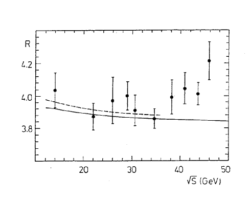
Figure 12: R measurements from PETRA and PEP experiments with the best fits of QED+QCD to all the data (full line) and only below $36\,$GeV (dashed line). All data points are correlated (see text).

To see the source of this effect more explicitly let us consider an alternative way often used to take the normalization uncertainty into account. A scale factor $f$, by which all data points are multiplied, is introduced to the expression of the $\chi^{2}$:

$$\chi^{2}_{A}=\frac{(f\cdot x_{1}-k)^{2}}{(f\cdot\sigma_{1})^{2}}+\frac{(f\cdot x_{2}-k)^{2}}{(f\cdot\sigma_{2})^{2}}+\frac{(f-1)^{2}}{\sigma_{f}^{2}}\,.$$ (272)

Let us also consider the same expression when the individual standard deviations are not rescaled:

$$\chi^{2}_{B}=\frac{(f\cdot x_{1}-k)^{2}}{\sigma_{1}^{2}}+\frac{(f\cdot x_{2}-k)^{2}}{\sigma_{2}^{2}}+\frac{(f-1)^{2}}{\sigma_{f}^{2}}\,.$$ (273)

The use of $\chi^{2}_{A}$ always gives the result $\widehat{k}=\overline{x}$, because the term $(f-1)^{2}/\sigma_{f}^{2}$ is harmless as far as the value of the minimum $\chi^{2}$ and the determination on $\widehat{k}$ are concerned. Its only influence is on $\sigma(\widehat{k})$, which turns out to be equal to quadratic combination of the weighted average standard deviation with $\sigma_{f}\cdot\overline{x}$, the normalization uncertainty on the average. This result corresponds to the usual one when the normalization factor in the definition of $\chi^{2}$ is not included, and the overall uncertainty is added at the end.

Instead, the use of $\chi^{2}_{B}$ is equivalent to the covariance matrix: the same values of the minimum $\chi^{2}$, of $\widehat{k}$ and of $\sigma(\widehat{k})$ are obtained, and $\widehat{f}$ at the minimum turns out to be exactly the $r$ ratio defined above. This demonstrates that the effect happens when the data values are rescaled independently of their standard uncertainties. The effect can become huge if the data show mutual disagreement. The equality of the results obtained with $\chi^{2}_{B}$ with those obtained with the covariance matrix allows us to study, in a simpler way, the behaviour of $r$ (= $\widehat{f}$) when an arbitrary amount of data points are analysed. The fitted value of the normalization factor is

$$\widehat{f}=\frac{1}{1+\sum_{i=1}^{n}\frac{(x_{i}-\overline{x})^{2}}{\sigma_{i}^{2}}\cdot\sigma_{f}^{2}}\,.$$ (275)

If the values of $x_{i}$ are consistent with a common true value it can be shown that the expected value of $f$ is

$$<f>=\frac{1}{1+(n-1)\cdot\sigma_{f}^{2}}\,.$$ (276)

Hence, there is a bias on the result when for a non-vanishing $\sigma_{f}$ a large number of data points are fitted. In particular, the fit on average produces a bias larger than the normalization uncertainty itself if $\sigma_{f}>1/(n-1)$. One can also see that $\sigma^{2}(\widehat{k})$ and the minimum of $\chi^{2}$ obtained with the covariance matrix or with $\chi^{2}_{B}$ are smaller by the same factor $r$ than those obtained with $\chi^{2}_{A}$.

16.2.4 Peelle’s Pertinent Puzzle

To summarize, where there is an overall uncertainty due to an unknown systematic error and the covariance matrix is used to define $\chi^{2}$, the behaviour of the fit depends on whether the uncertainty is on the offset or on the scale. In the first case the best estimates of the function parameters are exactly those obtained without overall uncertainty, and only the parameters’ standard deviations are affected. In the case of unknown normalization errors, biased results can be obtained. The size of the bias depends on the fitted function, on the magnitude of the overall uncertainty and on the number of data points.

It has also been shown that this bias comes from the linearization performed in the usual covariance propagation. This means that, even though the use of the covariance matrix can be very useful in analyzing the data in a compact way using available computer algorithms, care is required if there is one large normalization uncertainty which affects all the data.

The effect discussed above has also been observed independently by R.W. Peelle and reported the year after the analysis of the CELLO data[17]. The problem has been extensively discussed among the community of nuclear physicists, where it is presently known as “Peelle’s Pertinent Puzzle”[18].

A recent case in High Energy Physics in which this effect has been found to have biased the result is discussed in [19].

17 Multi-effect multi-cause inference: unfolding

17.1 Problem and typical solutions

In any experiment the distribution of the measured observables differs from that of the corresponding true physical quantities due to physics and detector effects. For example, one may be interested in measuring in the variables $x$ and $Q^{2}$ Deep Inelastic Scattering events. In such a case one is able to build statistical estimators which in principle have a physical meaning similar to the true quantities, but which have a non-vanishing variance and are also distorted due to QED and QCD radiative corrections, parton fragmentation, particle decay and limited detector performances. The aim of the experimentalist is to unfold the observed distribution from all these distortions so as to extract the true distribution (see also [20] and [21]). This requires a satisfactory knowledge of the overall effect of the distortions on the true physical quantity.

When dealing with only one physical variable the usual method for handling this problem is the so called bin-to-bin correction: one evaluates a generalized efficiency (it may even be larger than unity) calculating the ratio between the number of events falling in a certain bin of the reconstructed variable and the number of events in the same bin of the true variable with a Monte Carlo simulation. This efficiency is then used to estimate the number of true events from the number of events observed in that bin. Clearly this method requires the same subdivision in bins of the true and the experimental variable and hence it cannot take into account large migrations of events from one bin to the others. Moreover it neglects the unavoidable correlations between adjacent bins. This approximation is valid only if the amount of migration is negligible and if the standard deviation of the smearing is smaller than the bin size.

An attempt to solve the problem of migrations is sometimes made building a matrix which connects the number of events generated in one bin to the number of events observed in the other bins. This matrix is then inverted and applied to the measured distribution. This immediately produces inversion problems if the matrix is singular. On the other hand, there is no reason from a probabilistic point of view why the inverse matrix should exist. This as can easily be seen taking the example of two bins of the true quantity both of which have the same probability of being observed in each of the bins of the measured quantity. It follows that treating probability distributions as vectors in space is not correct, even in principle. Moreover the method is not able to handle large statistical fluctuations even if the matrix can be inverted (if we have, for example, a very large number of events with which to estimate its elements and we choose the binning in such a way as to make the matrix not singular). The easiest way to see this is to think of the unavoidable negative terms of the inverse of the matrix which in some extreme cases may yield negative numbers of unfolded events. Quite apart from these theoretical reservations, the actual experience of those who have used this method is rather discouraging, the results being highly unstable.

17.2 Bayes’ theorem stated in terms of causes and effects

Let us state Bayes’ theorem in terms of several independent causes ($C_{i},\ i=1,2,\ldots,n_{C}$) which can produce one effect ($E$). For example, if we consider Deep Inelastic Scattering events, the effect $E$ can be the observation of an event in a cell of the measured quantities $\{\Delta Q^{2}_{meas},\Delta x_{meas}\}$. The causes $C_{i}$ are then all the possible cells of the true values $\{\Delta Q^{2}_{true},\Delta x_{true}\}_{i}$. Let us assume we know the initial probability of the causes $P(C_{i})$ and the conditional probability that the $i$-th cause will produce the effect $P(E|C_{i})$. The Bayes formula is then

$$P(C_{i}|E)=\frac{P(E|C_{i})\cdot P(C_{i})}{\sum_{l=1}^{n_{C}}P(E|C_{l})\cdot P(C_{l})}\,.$$ (277)

$P(C_{i}|E)$ depends on the initial probability of the causes. If one has no better prejudice concerning $P(C_{i})$ the process of inference can be started from a uniform distribution.

The final distribution depends also on $P(E|C_{i})$. These probabilities must be calculated or estimated with Monte Carlo methods. One has to keep in mind that, in contrast to $P(C_{i})$, these probabilities are not updated by the observations. So if there are ambiguities concerning the choice of $P(E|C_{i})$ one has to try them all in order to evaluate their systematic effects on the results.

17.3 Unfolding an experimental distribution

If one observes $n(E)$ events with effect $E$, the expected number of events assignable to each of the causes is

$$\widehat{n}(C_{i})=n(E)\cdot P(C_{i}|E)\,.$$ (278)

As the outcome of a measurement one has several possible effects $E_{j}$ ($j=1,2,\ldots,n_{E}$) for a given cause $C_{i}$. For each of them the Bayes formula (277) holds, and $P(C_{i}|E_{j})$ can be evaluated. Let us write (277) again in the case of $n_{E}$ possible effects, indicating the initial probability of the causes with $P_{\circ}(C_{i})$:

$$P(C_{i}|E_{j})=\frac{P(E_{j}|C_{i})\cdot P_{\circ}(C_{i})}{\sum_{l=1}^{n_{C}}P(E_{j}|C_{l})\cdot P_{\circ}(C_{l})}\,.$$ (279)

One should note that:

• $\sum_{i=1}^{n_{C}}P_{\circ}(C_{i})=1$, as usual. Notice that if the probability of a cause is initially set to zero it can never change, i.e. if a cause does not exist it cannot be invented;

• $\sum_{i=1}^{n_{C}}P(C_{i}|E_{j})=1$  : this normalization condition, mathematically trivial since it comes directly from (279), indicates that each effect must come from one or more of the causes under examination. This means that if the observables also contain a non negligible amount of background, this needs to be included among the causes;

• $0\leq\epsilon_{i}\equiv\sum_{j=1}^{n_{E}}P(E_{j}|C_{i})\leq 1$ : there is no need for each cause to produce at least one of the effects. $\epsilon_{i}$ gives the efficiency of finding the cause $C_{i}$ in any of the possible effects.

After $N_{obs}$ experimental observations one obtains a distribution of frequencies $\underline{n}(E)\equiv\{n(E_{1}),n(E_{2}),\ldots,n(E_{n_{E}})\}$. The expected number of events to be assigned to each of the causes (taking into account only to the observed events) can be calculated applying (278) to each effect:

$$\left.\widehat{n}(C_{i})\right|_{obs} = \sum_{j=1}^{n_{E}}n(E_{j})\cdot P(C_{i}|E_{j})\,.$$ (280)

When inefficiency is also brought into the picture, the best estimate of the true number of events becomes

$$\widehat{n}(C_{i}) = \frac{1}{\epsilon_{i}}\sum_{j=1}^{n_{E}}n(E_{j})\cdot P(C_{i}|E_{j})\hskip 28.45274pt\epsilon_{i}\neq 0\,.$$ (281)

From these unfolded events we can estimate the true total number of events, the final probabilities of the causes and the overall efficiency:

$$\widehat{N}_{true} = \sum_{i=1}^{n_{C}}\widehat{n}(C_{i})$$

$$\widehat{P}(C_{i})\equiv P(C_{i}|\underline{n}(E)) = \frac{\widehat{n}(C_{i})}{\widehat{N}_{true}}$$

$$\widehat{\epsilon} = \frac{N_{obs}}{\widehat{N}_{true}}\,.$$

If the initial distribution $\underline{P_{\circ}}(C)$ is not consistent with the data, it will not agree with the final distribution $\underline{\widehat{P}}(C)$. The closer the initial distribution is to the true distribution, the better the agreement is. For simulated data one can easily verify for simulated data that the distribution $\underline{\widehat{P}}(C)$ lies between $\underline{P_{\circ}}(C)$ and the true one. This suggests proceeding iteratively. Fig.  13 shows an example of a bidimensional distribution unfolding.

More details about iteration strategy, evaluation of uncertainty, etc. can be found in [23].

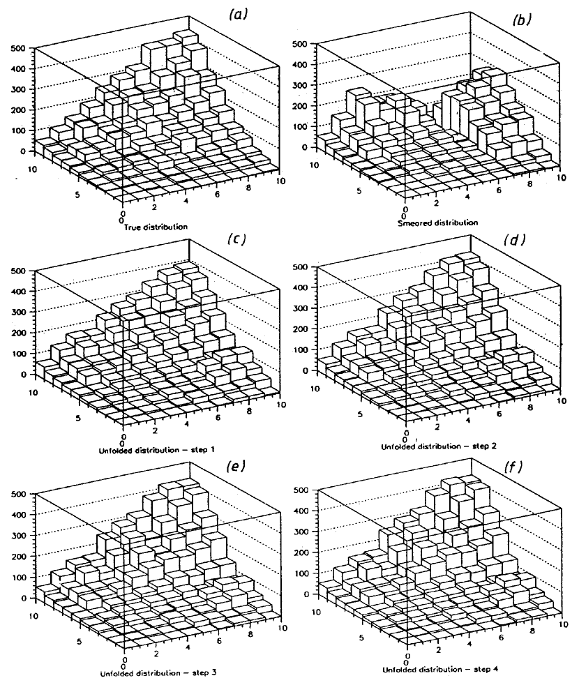
Figure 13: Example of a two dimensional unfolding: true distribution (a), smeared distribution (b) and results after the first 4 steps ((c) to (f)).

I would just like to comment on an obvious criticism that may be made: “the iterative procedure is against the Bayesian spirit, since the same data are used many times for the same inference”. In principle the objection is valid, but in practice this technique is a “trick” to give to the experimental data a weight (an importance) larger than that of the priors. A more rigorous procedure which took into account uncertainties and correlations of the initial distribution would have been much more complicated. An attempt of this kind can be found in [22]. Examples of unfolding procedures performed with non-Bayesian methods are described in [20] and [21].

18 Conclusions

These notes have shown how it is possible to build a powerful theory of measurement uncertainty starting from a definition of probability which seems of little use at first sight, and from a formula that - some say - looks too trivial to be called a theorem.

The main advantages the Bayesian approach has over the others are (further to the non negligible fact that it is able to treat problems on which the others fail):

• the recovery of the intuitive idea of probability as a valid concept for treating scientific problems;

• the simplicity and naturalness of the basic tool;

• the capability of combining prior prejudices and experimental facts;

• the automatic updating property as soon as new facts are observed;

• the transparency of the method which allows the different assumptions on which the inference may depend to be checked and changed;

• the high degree of awareness that it gives to its user.

When employed on the problem of measurement errors, as a special application of conditional probabilities, it allows all possible sources of uncertainties to be treated in the most general way.

When the problems get complicated and the general method becomes too heavy to handle, it is possible to use approximate methods based on the linearization of the final probability density function to calculate the first and second moments of the distribution. Although the formulae are exactly those of the standard “error propagation”, the interpretation of the true value as a random variable simplifies the picture and allows easy inclusion of uncertainties due to systematic effects.

Nevertheless there are some cases in which the linearization may cause severe problems, as shown in Section 14. In such cases one needs to go back to the general method or to apply other kinds of approximations which are not just blind use of the covariance matrix.

The problem of unfolding dealt with in the last section should to be considered a side remark with respect to the mainstream of the notes. It is in fact a mixture of genuine Bayesian method (the basic formula), approximations (covariance matrix evaluation) and ad hoc prescriptions of iteration and smoothing, used to sidestep the formidable problem of seeking the general solution.

I would like to conclude with three quotations:

• “($\ldots$) the best evaluation of the uncertainty ($\ldots$) must be given ($\ldots$)
  The method stands, therefore, in contrast to certain older methods that have the following two ideas in common:

  • The first idea is that the uncertainty reported should be ’safe’ or ’conservative’ ($\ldots$) In fact, because the evaluation of the uncertainty of a measurement result is problematic, it was often made deliberately large.

  • The second idea is that the influences that give rise to uncertainty were always recognizable as either ’random’ or ’systematic’ with the two being of different nature; ($\ldots$)”

  (ISO Guide[2])

• “Well, QED is very nice and impressive, but when everything is so neatly wrapped up in blue bows, with all experiments in exact agreement with each other and with the theory - that is when one is learning absolutely nothing.”

  “On the other hand, when experiments are in hopeless conflict - or when the observations do not make sense according to conventional ideas, or when none of the new models seems to work, in short when the situation is an unholy mess - that is when one is really making hidden progress and a breakthrough is just around the corner!”
  (R. Feynman, 1973 Hawaii Summer Institute, cited by D. Perkins at 1995 EPS Conference, Brussels)

• “Although this Guide provides a framework for assessing uncertainty, it cannot substitute for critical thinking, intellectual honesty, and professional skill. The evaluation of uncertainty is neither a routine task nor a purely mathematical one; it depends on detailed knowledge of the nature of the measurand and of the measurement. The quality and utility of the uncertainty quoted for the result of a measurement therefore ultimately depend on the understanding, critical analysis, and integrity of those who contribute to the assignment of its value”. (ISO Guide[2])

Bibliographic note

The state of the art of Bayesian theory is summarized in [7], where many references can be found. A concise presentation of the basic principles can instead been found in [24]. Text books that I have consulted are [4] and [6]. They contain many references too. As an introduction to subjective probability de Finetti’s “Theory of probability”[5] is a must. I have found the reading of [25] particular stimulating and that of [26] very convincing (thanks expecially to the many examples and exercises). Unfortunately these two books are only available in Italian for the moment.

Sections 6 and 7 can be reviewed in standard text books. I recommend those familiar to you.

The applied part of these notes, i.e. after section 9, is, in a sense, “original”, as it has been derived autonomously and, in many cases, without the knowledge that the results have been known to experts for two centuries. Some of the examples of section 13 were worked out for these lectures. The references in the applied part are given at the appropriate place in the text - only those actually used have been indicated. Of particular interest is the Weise and Wöger theory of uncertainty[14], which differs from that of these notes because of the additional use of the Maximum Entropy Principle.

A consultation of the ISO Guide[2] is advised. Presently the BIPM recommendations are also followed by the american National Institute of Standards and Technology (NIST), whose Guidelines[27] have the advantage, with respect to the ISO Guide, of being available on www too.

References

- [1] DIN Deutsches Institut für Normung, “Grunbegriffe der Messtechnick - Behandlung von Unsicherheiten bei der Auswertung von Messungen” (DIN 1319 Teile 1-4), Beuth Verlag GmbH, Berlin, Germany, 1985. Only parts 1-3 are published in English. An English translation of part 4 can be requested from the authors of [14]. Part 3 is going to be rewritten in order to be made in agreement with [2] (private communication from K. Weise).
- [2] International Organization for Standardization (ISO), “Guide to the expression of uncertainty in measurement”, Geneva, Switzerland, 1993.
- [3] H. Jeffreys, “Theory of probability”, Oxford University Press, 1961.
- [4] R. L. Winkler, “An introduction to Bayesian inference and decision”, Holt, Rinehart and Winston, Inc., 1972.
- [5] B. de Finetti, “Theory of probability”, J. Wiley & Sons, 1974.
- [6] S. J. Press, “Bayesian statistics: principles, models, and applications”, John Wiley & Sons Ltd, 1989.
- [7] J.M. Bernardo, A.F.M. Smith, “Bayesian theory”, John Wiley & Sons Ltd, Chichester, 1994.
- [8] Particle Data Group, “Review of particle properties”, Phys. Rev. D, 50 (1994) 1173.
- [9] New Scientist, April 28 1995, pag. 18 (“Gravitational constant is up in the air”). The data of Tab. 2 are from H. Meyer’s DESY seminar, June 28 1995.
- [10] P.L. Gaison, “How experiments end”, The University of Chicago Press, 1987.
- [11] G. D’Agostini, “Limits on electron compositeness from the Bhabha scattering at PEP and PETRA”, Proceedings of the th Rencontre de Moriond on “Z∘ Physics”, Les Arcs (France), March 4-11, 1990, pag. 229 (also DESY-90-093).
- [12] A.K. Wróblewski, ”Arbitrariness in the development of physics”, after-dinner talk at the International Workshop on Deep Inelastic Scattering and Related Subjects, Eilat, Israel, 6-11 February 1994, Ed. A. Levy (World Scientific, 1994), pag. 478.
- [13] E.T. Jaynes, “Information theory and statistical mechanics”, Phys. Rev. 106 (1957) 620.
- [14] K. Weise, W. Wöger, “A Bayesian theory of measurement uncertainty”, Meas. Sci. Technol., 4 (1993) 1.
- [15] International Organization for Standardization (ISO), “International vocabulary of basic and general terms in metrology”, Geneva, Switzerland, 1993.
- [16] G. D’Agostini, “On the use of the covariance matrix to fit correlated data”, Nucl. Instr. Meth. A346 (1994) 306.
- [17] CELLO Collaboration, H.J. Behrend et al., “Determination of and from measurements of total hadronic cross section in annihilation”, Phys. Lett. 183B (1987) 400.
- [18] S. Chiba and D.L. Smith, ”Impacts of data transformations on least-square solutions and their significance in data analysis and evaluation”, J. Nucl. Sc. Tech. 31 (1994) 770.
- [19] M. L. Swartz, “Reevaluation of the hadronic contribution to ”, SLAC-PUB-95-7001, September 1995, submitted to Phys. Rev. D.
- [20] V. Blobel, Proceedings of the “1984 CERN School of Computing”, Aiguablava, Catalonia, Spain, 9-12 September 1984, Published by CERN, July 1985, pag. 88-127.
- [21] G. Zech, “Comparing statistical data to Monte Carlo simulation - parameter fitting and unfolding”, DESY 95-113, June 1995.
- [22] K. Weise, “Matematical foundation of an analytical approach to bayesian Monte Carlo spectrum unfolding”, Physicalish Technische Bundesanstalt, Braunschweig, BTB-N-24, July 1995.
- [23] G. D’Agostini, “A multidimensional unfolding method based on Bayes’ theorem”, Nucl. Instr. Meth. A362 (1995) 487.
- [24] C. Howson and P. Urbach, “Bayesian reasoning in science”, Nature, Vol. 350, 4 April 1991, pag. 371.
- [25] B. de Finetti, “Filosofia della probabilità”, il Saggiatore, 1995.
- [26] R. Scozzafava, “La probabilità soggettiva e le sue applicazioni”, Masson, editoriale Veschi, Roma, 1993.
-
[27]
B.N. Taylor and C.E. Kuyatt,
“Guidelines for evaluating and expressing
uncertainty of NIST measurement results”, NIST Technical Note 1297,
September 1994;
(www: http://physics.nist.gov/Pubs/guidelines/outline.html).