HQET and Form Factor Effects in $B\to K^{(*)}\ell^{+}\ell^{-}$

Abstract

We examine the rates for the exclusive decays $B\to K^{(*)}\ell^{+}\ell^{-}$. We use the scaling predictions of the heavy quark effective theory to extract the necessary form factors from fits to various combinations of data. These data include the $D\to K^{(*)}\ell\nu$ semileptonic decays, as well as the nonleptonic decays $B\to K^{(*)}\psi^{(\prime)}$ and the rare decay $B\to K^{*}\gamma$. We use different parametrizations of form factors, and find that integrated decay rates are not very sensitive to the forms chosen. However, the decay spectra and the forward-backward asymmetry in $B\to K^{*}\ell^{+}\ell^{-}$ are sensitive to the forms chosen for the form factors, while the lepton polarization asymmetry in $\bar{B}^{0}\to\bar{K}^{0}\mu^{+}\mu^{-}$ is largely independent of the choice of form factors. Contributions from charmonium resonances dominate the spectra and integrated rates. In our ‘best’ scenario, we find $Br(\bar{B}^{0}\to\bar{K}^{0}\mu^{+}\mu^{-})=2.0\pm 0.3\times 10^{-6}$ and $Br(\bar{B}^{0}\to\bar{K}^{*0}\mu^{+}\mu^{-})=8.1\pm 2.0\times 10^{-6}$. We also make predictions for other polarization observables in these decays.

I Introduction

The rare dileptonic and radiative decays of $B$ mesons have been the subject of much recent interest. This is because the operators responsible for these decays are absent in the standard model at tree level, and first appear at one-loop level. As a result, these decays can provide sensitive tests of many issues, both within and beyond the standard model. The mass of the top quark and the Higgs boson, the existence or not of other Higgs multiplets, right-handed massive gauge bosons, or even extra left-handed massive gauge bosons, as well as questions concerning supersymmetric models are just some of the issues to which these decays are sensitive [1, 2, 3, 4, 5, 6, 7, 8, 9, 10, 11, 12, 13, 14, 15].

In order for these issues to be probed with any kind of precision in these decays, it is crucial that all of the long-distance effects be understood. At present, it is believed that this is the case for inclusive processes such as $B\to X_{s}\ell^{+}\ell^{-}$, the rates for which are taken to be the rates for the corresponding free-quark process. In this regard, the operator-product-expansion (OPE) of the heavy quark effective theory (HQET) has been used to treat inclusive decays beyond the free-quark approximation [1, 2, 16, 17]. This approximation is actually the leading term in a systematic expansion in the inverse of the $b$-quark mass, and becomes arbitrarily accurate as the mass of the $b$ quark approaches infinity. In addition, it has been shown that corrections to the free-quark picture first arise at order $1/m_{b}^{2}$, so that the predictions for the inclusive decay rates are expected to be quite reliable [16].

There are, however, two regions of phase space in which the OPE of HQET may be less reliable in predicting the inclusive decay rates [1]. The first is near the charmonium resonances, as the matrix elements of the four-quark operators that contribute in this region may be subject to large final state interactions. These may be beyond the scope of the HQET treatment of the inclusive process. The second is in the corner of phase space where $P_{X_{s}}^{2}\approx m_{s}^{2}$, where $P_{X_{s}}$ is the four-momentum of the hadronic final state $X_{s}$. This essentially arises from the fact that, for the free quark decay, the spectral end-point occurs at $P_{X_{s}}^{2}=m_{s}^{2}$, while for the case of real hadrons, it occurs at $P_{X_{s}}^{2}=m_{K}^{2}$. Apart from this, it is believed that the OPE of HQET provides a reliable description of the inclusive decays.

For the exclusive decays, the situation is not quite as rosy, as the free quark operators of the inclusive processes are replaced by hadronic matrix elements, which are described in terms of a number of a priori unknown, uncalculable, non-perturbative form factors. The dependence of these form factors on the appropriate kinematic variable may be modeled, but this muddles things as it introduces some model dependence in the extraction of information from the measured quantities.

In this regard, one may use the predictions of the heavy quark effective theory (HQET) [18, 19, 20, 21, 22, 23, 24, 25, 26, 27, 28, 29, 30, 31, 32] to relate the form factors for the exclusive rare decays of $B$ mesons to those of the semileptonic decays of $D$ mesons. There are two possible problems with this approach. The first is that the charm quark is not particularly heavy, and application of HQET to the decays of charmed mesons may be of questionable validity and value. The second is that to apply the form factors for the $D$ decays to $B$ decay processes requires extrapolation of the form factors well beyond the range that is kinematically accessible in $D$ decays.

Despite the relative ‘lightness’ of the $c$ quark, the predictions of HQET appear to be validated experimentally. For instance, the predictions for the decays of the $\Lambda_{c}$ [26, 33] are supported by experimental measurements [34, 35]. In addition, and perhaps more importantly, the predictions of HQET for the decays $B\to D\ell\nu$, in which the charm quark is treated as heavy, appear to be supported by experimental data. One may expect this success to carry over to the decays of charmed mesons, thus justifying the use of HQET for such decays.

The question of extrapolation of form factors is a delicate one. In a recent article, Roberts and Ledroit [32] have shown that depending on the choice of form factor parametrizations, as well as on the choice of form factor parameters, the form factors for $D$ decays may be applied with or without success to $B$ decays. The question of success or non-success was a crucial one for the nonleptonic decays $B\to K^{(*)}\psi^{(\prime)}$, for which the question of factorization or not of the matrix element is also of key importance. Similar results have been reported by other authors [36, 37, 38].

In [32], the authors found that all of the data treated, namely $D\to K^{(*)}\ell\nu$, $B\to K^{(*)}\psi^{(\prime)}$ and $B\to K^{*}\gamma$, could be described in terms of a single set of universal form factors. In this article, we use the results of that work to analyse the decays $B\to K\ell^{+}\ell^{-}$ and $B\to K^{*}\ell^{+}\ell^{-}$ in some detail, but concentrate on form factor effects rather than the effects of QCD coefficients, as these have been treated elsewhere by many authors. In the case of the latter process, we also examine the forward-backward asymmetry. In [32], effects due to charmonium resonances, and charm and light continua, were ignored. These are included in the present analysis.

The rest of this article is organized as follows. In the next section we discuss the standard model effective Hamiltonian for the rare dileptonic decays of interest, as well as the form factors for the exclusive decays, and their HQET relations to the form factors for the semileptonic decays of $D$ mesons. Our results for the total decay rates, spectra, forward-backward asymmetries and lepton polarization asymmetries are presented in section III, and section IV presents our conclusions.

II Effective Hamiltonian And Form Factors

A Rare Decays

In the standard model, the effective Hamiltonian for the decay $b\to s\ell^{+}\ell^{-}$ has the form

$${\cal H}_{\rm eff} = \frac{G_{F}}{\sqrt{2}}\frac{\alpha}{4\pi}V_{ts}^{*}V_{tb}\left[2i\frac{m_{b}}{q^{2}}C_{7}(m_{b})\bar{s}\sigma_{\mu\nu}q^{\nu}(1+\gamma_{5})b\bar{\ell}\gamma^{\mu}\ell\right.$$ (1)

$$+ \left.\vphantom{\frac{4G_{F}}{\sqrt{2}}}C_{9}(m_{b})\bar{s}\gamma_{\mu}\left(1-\gamma_{5}\right)b\bar{\ell}\gamma^{\mu}\ell+C_{10}(m_{b})\bar{s}\gamma_{\mu}\left(1-\gamma_{5}\right)b\bar{\ell}\gamma^{\mu}\gamma_{5}\ell\right],$$ (2)

where the Wilson coefficients $C_{i}(m_{b})$ are as in the article by Buras et al. [6]. We choose not to reproduce these coefficients here: the interested reader may consult the rich literature on this subject. We do point out, however, that $C_{9}$ and $C_{10}$ receive short distance contributions from the continua of light and charm $q\bar{q}$ pairs, as well as from charmonium resonances ($C_{9}$ only). This latter may be thought of as arising from the nonleptonic decay $B\to K^{(*)}\psi$, followed by the leptonic decay of the charmonium vector resonance, $\psi\to\ell^{+}\ell^{-}$. Thus, including these requires some assumption about the $B\to K^{(*)}\psi$ amplitude.

As has been done by other authors, we assume that this amplitude can be treated in the factorization approximation, so that the contribution from each charmonium vector resonance $V$ can be written as

$$C_{9}^{V}=\frac{16\pi^{2}}{3}\frac{V_{cb}V^{*}_{cs}}{V_{tb}V^{*}_{ts}}\left(\frac{f_{V}}{m_{V}}\right)^{2}\frac{a_{2}}{q^{2}-m_{V}^{2}+im_{V}\Gamma_{V}}.$$ (3)

Here, $m_{V}$ is the mass of the charmonium state, $\Gamma_{V}$ is its width, and $f_{V}$ is its decay constant. The constant $a_{2}$ is the phenomenological factorization constant, whose absolute value has been measured to be about 0.24. The sign of $a_{2}$ is still uncertain, so we explore the effects of changing this sign in the results that we present.

The hadronic matrix elements of the operators in eqn. (2) are

$$\left<K(p^{\prime})\left|\bar{s}\gamma_{\mu}c\right|B(p)\right> = f^{B}_{+}(p+p^{\prime})_{\mu}+f^{B}_{-}(p-p^{\prime})_{\mu},$$ (4)

$$\left<K(p^{\prime})\left|\bar{s}\gamma_{\mu}\gamma_{5}c\right|B(p)\right> = 0,$$ (5)

$$\left<K^{*}(p^{\prime},\epsilon)\left|\bar{s}\gamma_{\mu}c\right|B(p)\right> = ig^{B}\epsilon_{\mu\nu\alpha\beta}\epsilon^{*\nu}(p+p^{\prime})^{\alpha}(p-p^{\prime})^{\beta},$$ (6)

$$\left<K^{*}(p^{\prime},\epsilon)\left|\bar{s}\gamma_{\mu}\gamma_{5}c\right|B(p)\right> = f^{B}\epsilon^{*}_{\mu}+a^{B}_{+}\epsilon^{*}\cdot p(p+p^{\prime})_{\mu}+a^{B}_{-}\epsilon^{*}\cdot p(p-p^{\prime})_{\mu},$$ (7)

$$\left<K(p^{\prime})\left|\bar{s}\sigma_{\mu\nu}b\right|B(p)\right> = is^{B}\left[\left(p+p^{\prime}\right)_{\mu}\left(p-p^{\prime}\right)_{\nu}-\left(p+p^{\prime}\right)_{\nu}\left(p-p^{\prime}\right)_{\mu}\right],$$ (8)

$$\left<K^{*}(p^{\prime},\epsilon)\left|\bar{s}\sigma_{\mu\nu}b\right|B(p)\right> = \epsilon_{\mu\nu\alpha\beta}\left[g^{B}_{+}\epsilon^{*\alpha}\left(p+p^{\prime}\right)^{\beta}+g^{B}_{-}\epsilon^{*\alpha}\left(p-p^{\prime}\right)^{\beta}\right.$$ (10)

$$\left.+h^{B}\epsilon^{*}\cdot p\left(p+p^{\prime}\right)^{\alpha}\left(p-p^{\prime}\right)^{\beta}\right].$$

Due to the relation

$$\sigma^{\mu\nu}\gamma_{5}=\frac{i}{2}\varepsilon^{\mu\nu\alpha\beta}\sigma_{\alpha\beta},$$ (11)

we can easily relate the matrix elements involving $\sigma_{\mu\nu}$ to those in which the current is $\bar{s}\sigma_{\mu\nu}\gamma_{5}b$. The superscripts $B$ on the form factors signify that they are the ones appropriate to the decays of the $B$ mesons. These form factors may be related to the corresponding ones for decays of $D$ mesons, using the predictions of HQET.

The full formalism of HQET as it applies to these decays has been presented in [32]. Here, we briefly present the salient points of the discussion. In HQET, a heavy $B$ meson traveling with velocity $v$ is represented by the Dirac matrix [39]

$$B(v)\to\frac{1+v\hskip-5.0pt/}{2}\gamma_{5}.$$ (12)

The matrix elements of interest are then [32, 40]

$$\left<K(p)\left|\bar{s}\Gamma h_{v}^{(c)}\right|{\cal B}(v)\right> = {\rm Tr}\left\{\left(\xi_{1}+p\hskip-5.0pt/\xi_{2}\right)\gamma_{5}\Gamma\frac{1+v\hskip-5.0pt/}{2}\gamma_{5}\right\},$$ (13)

$$\left<K^{*}(p,\epsilon)\left|\bar{s}\Gamma h_{v}^{(c)}\right|{\cal B}(v)\right> = {\rm Tr}\left\{\left[\left(\xi_{3}+p\hskip-5.0pt/\xi_{4}\right)\epsilon^{*}\cdot v+\epsilon\hskip-5.0pt/^{*}\left(\xi_{5}+p\hskip-5.0pt/\xi_{6}\right)\right]\Gamma\frac{1+v\hskip-5.0pt/}{2}\gamma_{5}\right\},$$ (14)

where

$$\left|B(v)\right>=\sqrt{m_{B}}\left|{\cal B}(v)\right>.$$ (15)

These $\xi_{i}$ are independent of the masses of the heavy quarks and mesons, as well as of the exact form of the Dirac matrix $\Gamma$. Thus, they are valid for both $D\to K^{(*)}$ and $B\to K^{(*)}$, as well as for transitions mediated by vector, axial-vector and tensor currents.

The relationships between the form factors of eqn. (4) and the $\xi_{i}$ are

$$\xi_{1} = \frac{\sqrt{m_{B}}}{2}\left(f^{B}_{+}+f^{B}_{-}\right),$$ (16)

$$\xi_{2} = \frac{1}{2\sqrt{m_{B}}}\left(f^{B}_{-}-f^{B}_{+}\right)=-\sqrt{m_{B}}s^{B},$$ (17)

$$\xi_{3} = \frac{m_{B}^{3/2}}{2}\left(a^{B}_{+}+a^{B}_{-}\right),$$ (18)

$$\xi_{4} = \frac{\sqrt{m_{B}}}{2}\left(2g^{B}-a^{B}_{+}+a^{B}_{-}\right)=m_{B}^{3/2}h^{B},$$ (19)

$$\xi_{5} = -\frac{1}{2\sqrt{m_{B}}}\left(f^{B}+2m_{B}v\cdot pg^{B}\right)=-\frac{\sqrt{m_{B}}}{2}\left(g^{B}_{+}+g^{B}_{-}\right),$$ (20)

$$\xi_{6} = \sqrt{m_{B}}g^{B}=\frac{1}{2\sqrt{m_{B}}}\left(g^{B}_{-}-g^{B}_{+}\right).$$ (21)

The corresponding relationships for $D$ meson form factors require the replacement of all factors of $m_{B}$ in eqn. (16) by factors of $m_{D}$. Finally, we note that inclusion of radiative corrections requires the replacement [41]

$$\xi_{i}^{b\to s}=\xi_{i}^{c\to s}\left[\frac{\alpha_{s}(m_{b})}{\alpha_{s}(m_{c})}\right]^{-\frac{6}{25}}.$$ (22)

III Results And Discussion

All of the results we present are obtained by using the form factor parametrizations of [32]. In that work, two scenarios were explored for the form factors. In the first scenario, $\xi_{1}$ and $\xi_{4}$ had the form

$$\xi_{i}=a_{i}\exp{\left[-b_{i}\left(v\cdot p-m_{K^{(*)}}\right)^{2}\right]}=a_{i}\exp{\left[-\frac{b_{i}}{4m_{D}^{2}}\left(q^{2}_{{\rm max}}-q^{2}\right)^{2}\right]},$$ (23)

$\xi_{2}$ and $\xi_{5}$ had the form

$$\xi_{i}=a_{i}\exp{\left[-b_{i}\left(v\cdot p-m_{K^{(*)}}\right)\right]}=a_{i}\exp{\left[-\frac{b_{i}}{2m_{D}}\left(q^{2}_{{\rm max}}-q^{2}\right)\right]},$$ (24)

while $\xi_{5}$ and $\xi_{6}$ had the form

$$\xi_{i}=a_{i}\exp{\left[-b_{i}\left(v\cdot p\right)^{2}\right]}.$$ (25)

In the second scenario, the $\xi_{i}$ were parametrized as

$$\xi_{i}=a_{i}\left(1+b_{i}v\cdot p\right)^{n_{i}},$$ (26)

with $n_{i}=-2,\,-1,\,0,\,1$.

In each scenario, the $a_{i}$ and $b_{i}$ were free parameters that were fixed by fitting to various combinations of experimental measurements. Thus, for each scenario, four sets of $\{a_{i},b_{i}\}$ were generated. These corresponded to fits to (I) the semileptonic decays $D\to K^{(*)}\ell\nu$; (II) the semileptonic decays $D\to K^{(*)}\ell\nu$ and the nonleptonic decays $B\to K^{(*)}\psi$; (III) the semileptonic decays $D\to K^{(*)}\ell\nu$, the nonleptonic decays $B\to K^{(*)}\psi$ and the nonleptonic decays $B\to K^{(*)}\psi^{\prime}$; (IV) the semileptonic decays $D\to K^{(*)}\ell\nu$, the nonleptonic decays $B\to K^{(*)}\psi$, the nonleptonic decays $B\to K^{(*)}\psi^{\prime}$ and the rare decay $B\to K^{*}\gamma$. A fuller discussion of these fits and parameter sets is given in [32], but we emphasize that all of the results we present are obtained using form factors that are consistent at least with the measurements in $D\to K^{(*)}\ell\nu$, including polarization ratios. In addition, in this analysis, we have used $V_{tb}=0.9988$, $V_{ts}=0.03$, $V_{cs}=0.9738$, $V_{cb}=0.041$, $m_{b}=4.9$ GeV, $m_{c}$=1.5 GeV, $m_{t}$=177 GeV.

In fig. 1 we show our results for the rare dileptonic decays $B\to K^{(*)}\mu^{+}\mu^{-}$ using the form factors of the exponential scenario. Fig. 2 shows the corresponding spectra obtained using the form factors of the multipolar scenario. In each of figs. 1 and 2, the graph at the top left is $d\Gamma/dq^{2}$ for $B\to K\mu^{+}\mu^{-}$, while the second upper graph shows the spectrum for $B\to K^{*}\mu^{+}\mu^{-}$. The lower graphs show the corresponding curves for transversely and longitudinally polarized $K^{*}$’s in $B\to K^{*}\mu^{+}\mu^{-}$. For comparison, Fig. 3 shows the corresponding spectra for production of $\tau$ leptons, in the multipolar scenario.

The most dominant features of these curves are the sharp maxima due to the first two vector charmonium resonances. Apart from these two features, the spectra we have obtained are very similar to those obtained in [32]. In particular, the zeroes in some of the distributions still persist.

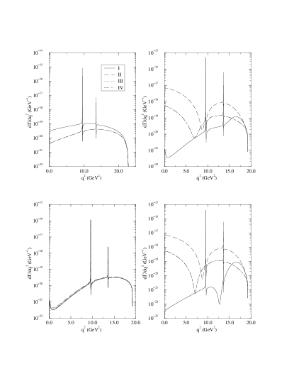
FIG. 1.: Differential decay rates for the processes $B\to K\mu^{+}\mu^{-}$ and $B\to K^{*}\mu^{+}\mu^{-}$, in the exponential scenario. The graphs are, starting at the top left and moving clockwise: $B\to K\mu^{+}\mu^{-}$; $B\to K^{*}\mu^{+}\mu^{-}$; $B\to K^{*}\mu^{+}\mu^{-}$ for longitudinally polarized $K^{*}$’s; $B\to K^{*}\mu^{+}\mu^{-}$ for transversely polarized $K^{*}$’s. In each graph, I means that the form factors used were obtained from a fit in which only data for $D\to K^{(*)}\ell\nu$ have been included; II means that data for $D\to K^{(*)}\ell\nu$ and $B\to K^{(*)}J/\psi$ have been included; III means that data for $D\to K^{(*)}\ell\nu$, $B\to K^{(*)}J/\psi$ and $B\to K^{(*)}\psi^{\prime}$ have been included; IV means that data for $D\to K^{*}\ell\nu$, $B\to K^{*}J/\psi$, $B\to K^{*}\psi^{\prime}$ and $B\to K^{*}\gamma$ have all been included, and does not apply to the process $B\to K\mu^{+}\mu^{-}$.

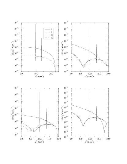
FIG. 2.: Differential decay rates for the processes $B\to K\mu^{+}\mu^{-}$ and $B\to K^{*}\mu^{+}\mu^{-}$, in the multipolar scenario. The graphs are, starting at the top left and moving clockwise: $B\to K\mu^{+}\mu^{-}$; $B\to K^{*}\mu^{+}\mu^{-}$; $B\to K^{*}\mu^{+}\mu^{-}$ for longitudinally polarized $K^{*}$’s; $B\to K^{*}\mu^{+}\mu^{-}$ for transversely polarized $K^{*}$’s. In each graph, the key is as in fig. 1.

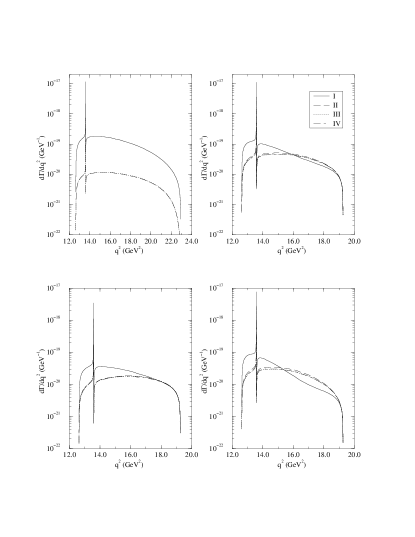
FIG. 3.: Differential decay rates for the processes $B\to K\tau^{+}\tau^{-}$ and $B\to K^{*}\tau^{+}\tau^{-}$, in the multipolar scenario. The graphs are, starting at the top left and moving clockwise: $B\to K\tau^{+}\tau^{-}$; $B\to K^{*}\tau^{+}\tau^{-}$; $B\to K^{*}\tau^{+}\tau^{-}$ for longitudinally polarized $K^{*}$’s; $B\to K^{*}\tau^{+}\tau^{-}$ for transversely polarized $K^{*}$’s. In each graph, the key is as in fig. 1.

The two charmonium resonances also dominate the total rates, as the numbers in tables I and II are all at least twice as large as the corresponding numbers reported in [32], where the resonance effects were not included. In these tables, the labels of the columns correspond to the fits described above. This means, for instance, that the predictions of set III are obtained using the form factors from fit III, in which we have included the data for the semileptonic decays $D\to K^{(*)}\ell\nu$, the nonleptonic decays $B\to K^{(*)}\psi$ and the nonleptonic decays $B\to K^{(*)}\psi^{\prime}$. The errors that we quote in all of the numbers we report are estimates only, and are obtained by using the covariance matrix that arises from the fit.

TABLE I.: Predictions for decay rates of $B\to K^{(*)}\mu^{+}\mu^{-}$ in the exponential scenario. I means that only $D\to K^{(*)}\ell\nu$ has been included in the fit; II means $D\to K^{(*)}\ell\nu$ and $B\to K^{(*)}J/\psi$ have been included; III means $D\to K^{(*)}\ell\nu$, $B\to K^{(*)}J/\psi$ and $B\to K^{(*)}\psi^{\prime}$ have been included; IV means $D\to K^{*}\ell\nu$, $B\to K^{*}J/\psi$, $B\to K^{*}\psi^{\prime}$ and $B\to K^{*}\gamma$ have all been included, and applies only to decays with $K^{*}$’s in the final state.

Quantity	Experiment	I	II	III	IV
$\Gamma_{B\to K\mu^{+}\mu^{-}}$ ($10^{-18}$ GeV)	$<158.0$	$2.32\pm 4.46$	$0.78\pm 0.19$	$0.78\pm 0.19$	-
$\Gamma_{B\to K^{*}\mu^{+}\mu^{-}}^{T}$ ($10^{-18}$ GeV)	-	$0.39\pm 0.22$	$0.42\pm 0.10$	$0.41\pm 0.08$	$0.41\pm 0.09$
$\Gamma_{B\to K^{*}\mu^{+}\mu^{-}}^{L}$ ($10^{-18}$ GeV)	-	$0.28\pm 0.07$	$28.9\pm 20.3$	$2.47\pm 0.32$	$2.46\pm 2.65$
$\Gamma_{B\to K^{*}\mu^{+}\mu^{-}}$ ($10^{-18}$ GeV)	$<10.1$	$0.67\pm 0.22$	$29.4\pm 20.3$	$2.88\pm 0.28$	$2.88\pm 2.65$

TABLE II.: Predictions for decay rates of $B\to K^{(*)}\mu^{+}\mu^{-}$ in the multipolar scenario. The columns are as in table I.

Quantity	Experiment	I	II	III	IV
$\Gamma_{B\to K\mu^{+}\mu^{-}}$ ($10^{-18}$ GeV)	$<158.0$	$1.86\pm 1.59$	$0.86\pm 0.15$	$0.87\pm 0.15$	-
$\Gamma_{B\to K^{*}\mu^{+}\mu^{-}}^{T}$ ($10^{-18}$ GeV)	-	$10.8\pm 2.18$	$0.69\pm 0.14$	$0.69\pm 0.17$	$0.60\pm 0.06$
$\Gamma_{B\to K^{*}\mu^{+}\mu^{-}}^{L}$ ($10^{-18}$ GeV)	-	$142.8\pm 28.5$	$3.54\pm 2.48$	$2.86\pm 2.07$	$2.93\pm 0.89$
$\Gamma_{B\to K^{*}\mu^{+}\mu^{-}}$ ($10^{-18}$ GeV)	$<10.1$	$153.6\pm 28.4$	$4.22\pm 2.48$	$3.56\pm 2.07$	$3.52\pm 0.89$

Apart from the charmonium features shown in these figures, the differences in the predicted spectra for different parametrizations of form factors, but within the same scenario, and from the exponential to the multipolar scenario, are quite striking. The reader is reminded that for all of these curves, the form factors are consistent with all of the measurements in the semileptonic decays $D\to K^{*}\ell\nu$. Nevertheless, apart from a few obvious exceptions, the predictions for the total rates are surprisingly similar for the different parametrizations and scenarios.

If the final leptons are electrons, all of the curves we have shown are essentially the same, with the exception of those for transversely polarized $K^{*}$’s for small $q^{2}$ (and consequently, for unpolarized $K^{*}$’s as well). This is because the differential decay rate for transversely polarized $K^{*}$’s behaves like $1/q^{2}$ for small $q^{2}$, and the different end-points for electrons and muons means that the spectra are different at small $q^{2}$. In fact, the $1/q^{2}$ dependence is softened by a factor of $\sqrt{q^{2}-4m_{\ell}^{2}}$ in the decay rate. That phase space extends further for electron pairs has essentially no impact on the rate for $B\to K\ell^{+}\ell^{-}$, nor for longitudinally polarized $K^{*}$’s in $B\to K^{*}\ell^{+}\ell^{-}$. However, there is a significant increase in the rate for transversely polarized $K^{*}$’s, with a slightly less significant effect for unpolarized $K^{*}$’s. This is seen by comparing the numbers in tables II and III. The effect is also shown in fig. 4. For tau leptons, all rates are smaller by about an order of magnitude.

TABLE III.: Predictions for decay rates of $B\to K^{(*)}e^{+}e^{-}$ in the multipolar scenario. The columns are as in table I.

Quantity	Experiment	I	II	III	IV
$\Gamma_{B\to Ke^{+}e^{-}}$ ($10^{-18}$ GeV)	$<158.0$	$1.87\pm 1.60$	$0.86\pm 0.15$	$0.87\pm 0.15$	-
$\Gamma_{B\to K^{*}e^{+}e^{-}}^{T}$ ($10^{-18}$ GeV)	-	$15.7\pm 3.29$	$1.07\pm 0.36$	$1.09\pm 0.42$	$0.74\pm 0.08$
$\Gamma_{B\to K^{*}e^{+}e^{-}}^{L}$ ($10^{-18}$ GeV)	-	$144.7\pm 28.9$	$3.59\pm 2.52$	$2.90\pm 2.11$	$2.96\pm 0.91$
$\Gamma_{B\to K^{*}e^{+}e^{-}}$ ($10^{-18}$ GeV)	$<10.1$	$160.4\pm 28.7$	$4.66\pm 2.53$	$4.00\pm 2.14$	$3.70\pm 0.90$

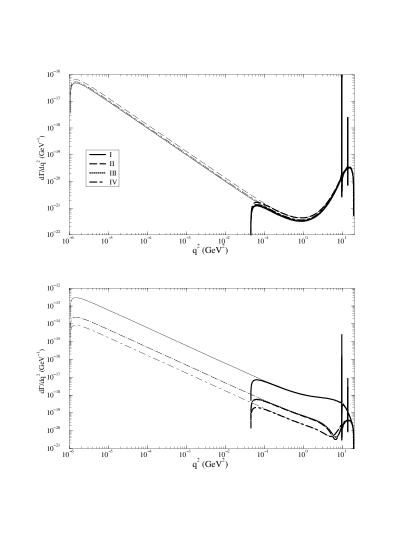
FIG. 4.: Differential decay rates for the processes $B\to K^{*}\mu^{+}\mu^{-}$ and $B\to K^{*}e^{+}e^{-}$, for transversely polarized $K^{*}$’s. The exponential scenario is the upper graph, while the multipolar scenario is the lower graph. In each graph, the thick curves are for $B\to K^{*}\mu^{+}\mu^{-}$, while the thin curves are for $B\to K^{*}e^{+}e^{-}$, and the key is as in fig. 1.

In addition to the differential decay rate, there are two other quantities of interest for these decays. One is the differential forward-backward asymmetry, $A_{{\rm FB}}$, which may be defined as

$$A_{{\rm FB}}=\frac{\int^{1}_{0}\frac{d\Gamma}{dq^{2}d\cos{\theta_{\ell}}}d\cos{\theta_{\ell}}-\int^{0}_{-1}\frac{d\Gamma}{dq^{2}d\cos{\theta_{\ell}}}d\cos{\theta_{\ell}}}{\int^{1}_{0}\frac{d\Gamma}{dq^{2}d\cos{\theta_{\ell}}}d\cos{\theta_{\ell}}+\int^{0}_{-1}\frac{d\Gamma}{dq^{2}d\cos{\theta_{\ell}}}d\cos{\theta_{\ell}}}.$$ (27)

Here, $\theta_{\ell}$ is the angle that the negatively charged lepton makes, in the dilepton rest frame, with the momentum of the daughter $K^{*}$, and the denominator is simply $d\Gamma/dq^{2}$. This quantity is identically zero, in the standard model, for $B\to K\ell^{+}\ell^{-}$.

The forward-backward asymmetries that result from our calculations are shown in fig. 5 for $B\to K^{*}\mu^{+}\mu^{-}$, and in figure 6 for $B\to K^{*}\tau^{+}\tau^{-}$. In each case, the upper graph is for the exponential scenario, while the lower one is for the multipolar one. We again emphasize that the differences in the curves for each graph arise from changes in the parameters of the form factors. We also point out that the form of this asymmetry will also depend on the physics content of the Wilson coefficients, and that the curves shown all correspond to standard-model physics only.

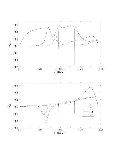
FIG. 5.: The forward-backward asymmetry, $A_{{\rm FB}}$, in $B\to K^{*}\mu^{+}\mu^{-}$. The upper graph is for the exponential scenario, while the lower is for the multipolar scenario. In each graph, the key is as in fig. 1.

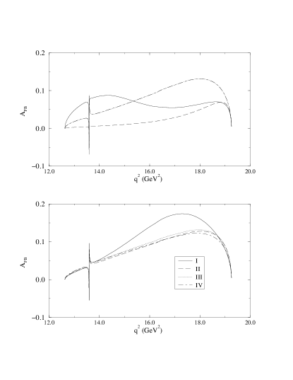
FIG. 6.: The forward-backward asymmetry, $A_{{\rm FB}}$, in $B\to K^{*}\tau^{+}\tau^{-}$. The upper graph is for the exponential scenario, while the lower is for the multipolar scenario. In each graph, the key is as in fig. 1.

The second quantity of interest in these decays is the lepton polarization asymmetry, defined as

$${\cal P}_{\ell}=\frac{\left.\frac{d\Gamma}{dq^{2}}\right|_{\lambda=-1}-\left.\frac{d\Gamma}{dq^{2}}\right|_{\lambda=+1}}{\left.\frac{d\Gamma}{dq^{2}}\right|_{\lambda=-1}+\left.\frac{d\Gamma}{dq^{2}}\right|_{\lambda=+1}},$$ (28)

where the subscripts $\lambda$ denote whether the spin of the $\ell^{-}$ is alligned parallel ($\lambda=+1$) or antiparallel ($\lambda=-1$) to its motion. Fig. 7 shows the results we obtain for this quantity for muons in $B\to K\mu^{+}\mu^{-}$, while fig. 8 shows the corresponding results for $B\to K^{*}\mu^{+}\mu^{-}$. Figs. 9 and 10, respectively, show the corresponding results for tau leptons.

The most striking feature of fig. 7 is the insensitivity of ${\cal P}_{\mu}$ to the parametrization of the form factors. The same feature also appears in fig. 8, but mainly for the large dilepton mass region of phase space. The insensitivity of this polarization observable to form factors has not previously been anticipated as far as we know, and suggests that the polarization asymmetry could be one of the more useful observables for examining the physics content of the Wilson coefficients.

This asymmetry in $B\to K\ell^{+}\ell^{-}$ is independent of form factor parametrizations due to a combination of two effects. The first of these is the small lepton mass (for $\ell=\mu$ or $e$), which means that many terms in the differential decay rate are small for most regions of phase space. The second is the relative smallness of the $C_{7}$ coefficient compared with $C_{9}$ and $C_{10}$. The consequence of this, together with the small lepton mass, is that any form factor dependence in the polarization asymmetry disappears. In fact, to a very good approximation, in the limit in which $C_{7}$ is small, we find

$${\cal P}_{\mu}\approx 2\frac{{\rm Re}C_{9}C_{10}^{*}}{\left|C_{9}\right|^{2}+\left|C_{10}\right|^{2}}+{\cal O}\left(C_{7}\right).$$ (29)

This is also independent of the assumptions of HQET, since only the hadronic vector and axial vector operators contribute to ${\cal P}_{\mu}$: eqn. (29) does not rely on any special relationships among form factors. This asymmetry therefore provides a direct measure of the interference between $C_{9}$ and $C_{10}$. In addition, experimental observation of significant departures from this nearly constant value for muons would signal larger values of $C_{7}$, and therefore, possibly, new physics.

Figure 8 shows a similar effect in the polarization of the muons produced in $B\to K^{*}\mu^{+}\mu^{-}$, particularly at large values of the dilepton mass. In fact, to the same level of approximation, the lepton polarization in this process is given by the same expression, eqn. (29). This is a better approximation at large values of $q^{2}$, as form factor effects become more significant at smaller $q^{2}$ for this decay.

Unfortunately, in the case of $\tau$ leptons, where the polarization may be more easily measured, the fact that the lepton mass is large means that this polarization variable depends on the particular choice of form factors, as can be seen in figs. 9 and 10. Nevertheless, some simplification does occur at the kinematic end-point, where $q^{2}=q^{2}_{\rm max}$. There, form factor dependence again disappears, and the tau polarization asymmetry is determined solely in terms of the coefficients $C_{9}$ and $C_{10}$ (assuming that $C_{7}$ is small), and the hadron and lepton masses, $m_{B}$, $m_{K^{*}}$ and $m_{\tau}$ (at this kinematic point in $B\to K\ell^{+}\ell^{-}$, the polarization asymmetry vanishes identically). Thus, for given values of the Wilson coefficients, there is a firm prediction for this asymmetry at maximum $q^{2}$ in $B\to K^{*}\tau^{+}\tau^{-}$. We note that the form of the curve we obtain for this quantity in the exclusive channel $B\to K^{*}\tau^{+}\tau^{-}$ is very similar to that obtained by Hewett [42] in the inclusive process $B\to X_{s}\tau^{+}\tau^{-}$.

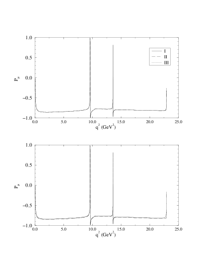
FIG. 7.: The lepton polarization asymmetry, ${\cal P}_{\mu}$, in $B\to K\mu^{+}\mu^{-}$. The upper graph is for the exponential scenario, while the lower is for the multipolar scenario. In each graph, the key is as in fig. 1. The curves for the different fits are essentially indistinguishable on this scale.

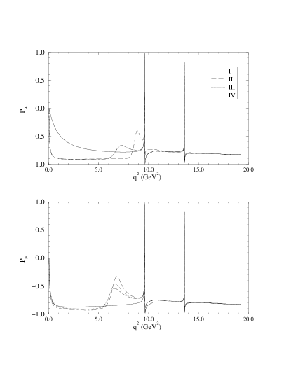
FIG. 8.: The lepton polarization asymmetry, ${\cal P}_{\mu}$, in $B\to K^{*}\mu^{+}\mu^{-}$. The upper graph is for the exponential scenario, while the lower is for the multipolar scenario. In each graph, the key is as in fig. 1.

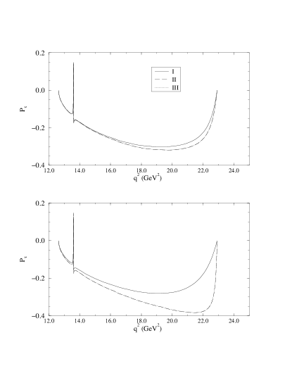
FIG. 9.: The lepton polarization asymmetry, ${\cal P}_{\tau}$, in $B\to K\tau^{+}\tau^{-}$. The upper graph is for the exponential scenario, while the lower is for the multipolar scenario. In each graph, the key is as in fig. 1.

FIG. 10.: The lepton polarization asymmetry, ${\cal P}_{\tau}$, in $B\to K^{*}\tau^{+}\tau^{-}$. The upper graph is for the exponential scenario, while the lower is for the multipolar scenario. In each graph, the key is as in fig. 1.

Finally, we turn to the question of the sign of $a_{2}$. Since this parameter enters only through the charmonium resonances, it should not be surprising that the effects of a change in its sign are most clearly visible in the vicinity of these resonances. In the decay spectra, there is some modification of the shape, but only very close to each resonance. The effect on $A_{{\rm FB}}$ is a little more interesting, and is displayed in fig. 11. However, since the difference between the two sets of curves shown occurs between $q^{2}$ of 9.52 and 9.64 GeV², it is doubtful whether future experiments will ever have the $q^{2}$ resolution needed to distinguish one set of curves from the other. Thus, we would suggest that the prospects of determining the sign of $a_{2}$ from these decays are not very promising. We find a similar result when we examine the effect of the sign of $a_{2}$ on the lepton polarization asymmetry.

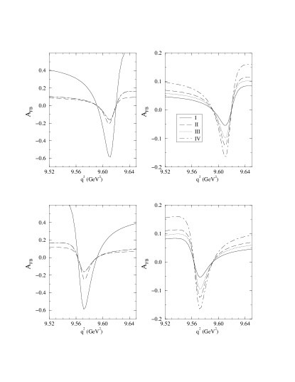
FIG. 11.: The effect of the sign of $a_{2}$ on $A_{{\rm FB}}$ in $B\to K^{*}\ell^{+}\ell^{-}$. The two graphs on the left are for the exponential scenario, while the two on the right are for the multipolar scenario. The two upper graphs are for $a_{2}>0$, while the two lower ones are for $a_{2}<0$. In each graph, the key is as in fig. 1.

Our predictions for the process $B\to K\ell^{+}\ell^{-}$ are two to three orders of magnitude smaller than present experimental upper limits, but they are about three times as large as the rates predicted by Ali et al. [3]. Our absolute rates correspond to branching fractions of $(1.8\pm 0.4)\times 10^{-6}$ in the exponential scenario, and $(2.0\pm 0.3)\times 10^{-6}$ in the multipolar scenario.

For $B\to K^{*}\ell^{+}\ell^{-}$ our predicted branching fractions are $(6.6\pm 0.8)\times 10^{-6}$ and $(8.1\pm 2.0)\times 10^{-6}$ in the exponential and multipolar scenarios, respectively, for muon pairs. For electron pairs, the multipolar scenario predicts a branching fraction of $(8.5\pm 2.1)\times 10^{-6}$. Furthermore, we find the ratio $\Gamma_{T}/\Gamma_{L}$ in $B\to K^{*}\mu^{+}\mu^{-}$ to be $0.17\pm 0.06$ in the exponential scenario and $0.20\pm 0.08$ in the multipolar scenario. For $B\to K^{*}e^{+}e^{-}$, the multipolar scenario predicts a value of $0.25\pm 0.10$ for this quantity. It is somewhat surprising but nonetheless reassuring that even this polarization ratio is largely independent of form factor parametrizations. This suggests that our predictions for total rates should be quite reliable, as uncertainties due to form factor parametrizations have less impact on integrated quantities.

The numbers that we have quoted for $B\to K^{*}\ell^{+}\ell^{-}$ correspond to III of the exponential scenario and IV of the multipolar scenario. In the case of the exponential scenario, we have chosen III as the best numbers to present for two related reasons. The first is that the theoretical uncertainties on IV are unreasonably large, while those on III are more ‘reasonable’. However, as can be seen from the graphs (and the tables), there is very little difference between III and IV in this scenario. The problem arises because in going from III to IV, we have added the CLEO measurement of $B\to K^{*}\gamma$ to the fit, and the exponential scenario can not accomodate the experimental measurement (the ‘best fit’ in this scenario is more than a factor of 100 smaller than the measurement). Consequently, the fit parameters (and our predictions) remain the same in going from III to IV, but the errors on the predictions have increased. In contrast with this, IV of the multipolar scenario provides a satisfactory description of all the data used in the fit, including the measured rate for $B\to K^{*}\gamma$.

IV Conclusion

There is a plethora of issues that we have not touched in this note. Extensions to the standard model and their effects on the Wilson coefficients, scale dependence of these coefficients, and the forms of these coefficients at leading order and beyond are beyond the scope of this article. While these issues are very important, recent calculations suggest that, at least for the inclusive decays, some kind of convergence is at hand. This is not so for the exclusive decays. Our results indicate that while results for integrated rates and lepton polarization asymmetries appear to be largely independent of the parametrization chosen for the form factors, differential rates and the forward-backward asymmetry are not. Measurements of these quantities in exclusive channels will therefore serve to probe form factor models or parametrizations. This is therefore similar to the situation in the exclusive decay $B\to K^{*}\gamma$, which has turned out to be a testing ground for form factor models.

The scenario that best describes all of the experimental data is the multipolar one and, in this scenario, we find that the universal form factor $\xi_{6}$ is linear in $v\cdot p$. Using this scenario, we predict $Br(\bar{B}^{0}\to\bar{K}^{0}\mu^{+}\mu^{-})=(2.0\pm 0.3)\times 10^{-6}$ and $Br(\bar{B}^{0}\to\bar{K}^{*0}\mu^{+}\mu^{-})=(8.1\pm 2.0)\times 10^{-6}$. These numbers are consistent with other model calculations [10], and include the effects of the first two charmonium vector resonances. We also predict $\Gamma_{T}/\Gamma_{L}$ in $\bar{B}^{0}\to\bar{K}^{*0}\mu^{+}\mu^{-}$ to be $0.20\pm 0.08$.

In the course of this study we have discovered that the polarization asymmetries in the decays $B\to K^{(*)}\mu^{+}\mu^{-}$ are, to a very good approximation, independent of form factor effects, and are determined solely in terms of the Wilson coefficients $C_{9}$ and $C_{10}$. This is particularly so for the decays to the ground state kaons, as the approximation is valid over all of phase space. Thus, these observables could be very useful tools for probing the physics content of the Wilson coefficients. However, in order for this to be a practical tool, experimentalists must be able to measure the polarization of the daughter muons in these decays, with adequate precision.

Hewett [42] suggests that the polarization of the tau leptons could be measurable at $B$ factories that are under construction. If that is the case, there should certainly be sufficient numbers of events produced in the muon channels, at least in the ‘clean’ region away from the two charmonium resonances, as the decay rates for muons and taus are comparable in this region of phase space. The remaining question is therefore simply one of whether the polarization of the muon can be measured in these decays. This may be possible for sufficiently slow muons, or if the muons can be stopped in the detector.

For tau leptons, simplifications such as those mentioned above do not occur, and the polarization asymmetry depends on form factors for almost all of phase space. The sole exception is at the kinematic end point in the decay $B\to K^{*}\tau^{+}\tau^{-}$, when the dilepton pair has maximum $q^{2}$. There, for given values of the Wilson coefficients, there is a firm prediction for this asymmetry in $B\to K^{*}\tau^{+}\tau^{-}$. We emphasize again that the fact that the asymmetry is independent of form factors does not depend on the assumptions of the heavy quark effective theory. Whether either of these polarization effects can ever be measured will have to await completion of the $B$ factories.

REFERENCES

• [1] A. F. Falk, M. Luke and M. J. Savage, Phys. Rev. D49 (1994) 3367.
• [2] A. Ali, G. F. Giudice and T. Mannel, Z.Phys. C67 (1995) 417.
• [3] A. Ali, C. Greub and T. Mannel in Proceedings of ECFA Workshop on the Physics of a B Meson Factory, R. Aleksan and A. Ali, eds. 1993.
• [4] The articles in B Decays, World Scientific (1992), Sheldon Stone, ed., contain many references to the relevant heavy quark literature.
• [5] D. - S. Liu, UTAS-PHYS-95-08, unpublished; Phys. Lett. B346 (1995) 355.
• [6] A. J. Buras and M. MΓΌnz, Phys. Rev. D52 (1995) 186.
• [7] N. G. Deshpande in B Decays, World Scientific (1992), Sheldon Stone, ed.
• [8] G. Burdman, FERMILAB-PUB-95-113-T, unpublished.
• [9] W. S. Hou, R. I. Willey and A. Soni, Phys. Rev. Lett. 58 (1987) 1608; B. Grinstein, M. J. Savage and M. B. Wise, Nucl. Phys. B319 (1989) 271; M. Misiak, Nucl. Phys. B393 (1993) 23; M. Misiak, Erratum, Nucl. Phys. B395 (1995) 461; R. Grigjanis, P. J. O’Donnell, M. Sutherland and H. Navelet, Phys. Rep. 228 (1993) 93.
• [10] S. Playfer and S. Stone, to appear in International Journal of Modern Physics Letters.
• [11] G. Ricciardi, DSF-T-95/39, unpublished.
• [12] P. Colangelo et al., BARI-TH/95-206, unpublished.
• [13] M. R. Ahmady, OCHA-PP-64, unpublished.
• [14] M. R. Ahmady, D. - S. Liu and A. H. Fariborz, HEPPH-9506235, unpublished.
• [15] A. Ali and T. Mannel, Phys. Lett. B264 (1991) 447; Erratum, ibid B274 (1992) 526; A. Ali, T. Ohl and T. Mannel, Phys. Lett. B298 (1993) 195.
• [16] J. Chay, H. Georgi and B. Grinstein, Phys. Lett. B247 (1990) 399.
• [17] I. Bigi, N. Uraltsev, A. Vainshtein Phys. Lett. B293 (1992) 430; B. Blok and M. Shifman, Nucl. Phys. B399 (1993) 441, 459; I. Bigi, B. Blok, M. Shifman, N. Uraltsev, A. Vainshtein, The Fermilab Meeting Proc. of the 1992 DPF meeting of APS, C.H. Albright et al., Eds. World Scientific, Singapore, 1993, vol.1, p. 610; I. Bigi, M. Shifman, N. Uraltsev and A. Vainshtein, Phys. Rev. Lett. 71 (1993) 496; B. Blok, L. Koyrakh, M. Shifman, A. Vainshtein, Phys. Rev. D49 (1994) 3356; A. Manohar and M. Wise, Phys. Rev. D49 (1994) 1310.
• [18] N. Isgur and M. Wise, Phys. Lett. B232 (1989) 113; Phys. Lett. B237 (1990) 527.
• [19] B. Grinstein, Nucl. Phys. B339 (1990) 253.
• [20] H. Georgi, Phys. Lett. B240 (1990) 447.
• [21] A. Falk, H. Georgi, B. Grinstein and M. Wise, Nucl. Phys. B343 (1990) 1.
• [22] A. Falk and B. Grinstein, Phys. Lett. B247 (1990) 406.
• [23] T. Mannel, W. Roberts and Z. Ryzak, Nucl. Phys. B368 (1992) 204.
• [24] M. Luke, Phys. Lett. B252 (1990) 447.
• [25] A. Falk, B. Grinstein and M. Luke, Nucl. Phys. B357 (1991) 185.
• [26] T. Mannel, W. Roberts and Z. Ryzak, Nucl. Phys. B355 (1991) 38.
• [27] N. Isgur and M. B. Wise, Nucl. Phys. B348 (1991) 276.
• [28] H. Georgi, Nucl. Phys. B348 (1991) 293.
• [29] M. Neubert, Phys. Rep. 245 (1994) 259, and references therein.
• [30] N. Isgur and M. B. Wise, Phys. Rev. D42 (1991) 2388.
• [31] See for example, H. Georgi, in Proceedings of TASI-91, A. J. Buras and M. Lindner, eds.; B. Grinstein in TASI-94 (1994); W. Roberts, in Physics In Collision 14, S. Keller and H. D. Wahl, eds.
• [32] W. Roberts and F. Ledroit, CEBAF preprint TH-95-02, unpublished.
• [33] T. Mannel, W. Roberts and Z. Ryzak, Phys. Lett. B259 (1991) 485; Phys. Lett. B255 (1991) 593.
• [34] H. Albrecht et al., Phys. Lett. B326 (1994) 320; T. Bergfeld et al., Phys. Lett. B323 (1994) 219.
• [35] H. Albrecht et al., Phys. Lett. B274 (1992) 239; P. Avery et al., Phys. Lett. B325 (1994) 257.
• [36] M. Gourdin, A.N. Kamal and X.Y. Pham, Phys. Rev. Lett. 73 (1994) 3355; M. Gourdin, Y.Y. Keum and X.Y. Pham, Phys. Rev. D52 (1995) 185; PAR-LPTHE-94-44, unpublished.
• [37] R. Aleksan, A. Le Yaouanc, L. Oliver, O. Pene and J.C. Raynal, Phys. Rev. D51 (1995) 6235; LPTHE-ORSAY-94-105, unpublished.
• [38] C. Carlson and J. Milana, WM-94-110, unpublished.
• [39] A. Falk, Nucl. Phys. B378 (1992) 79.
• [40] T. Mannel and W. Roberts, Z. Phys. C61 (1994) 293.
• [41] M. A. Shifman and M. B. Voloshin, Sov. J. Nucl. Phys. 45 (1987) 292; H. D. Politzer and M. B. Wise, Phys. Lett. B206 (1988) 681; H. D. Politzer and M. B. Wise, Phys. Lett. B208 (1988) 504; E. Eichten and B. Hill, Phys. Lett. B234 (1990) 511.
• [42] J. L. Hewett, SLAC-PUB-95-6820, unpublished.