Axionic Extensions of the Standard Model

Abstract

After a brief review of the axion solution of the strong CP problem, its supersymmetric extension and the superstring axion are discussed. I also present one interesting cosmological scenario, the axino-gravitino cosmology, for the large scale structure of the universe.

1 The Axion Solution of the Strong CP Problem

The standard model describes the low energy phenomena very successfully with 19 free parameters given by

$${\rm Gauge\ sector}\ :\ \alpha_{3},\ \alpha_{2},\ \alpha_{1},\ M_{W},\ M_{Z}$$

$${\rm Higgs\ potential}\ :\ \lambda,\ M_{H}^{2}$$

$${\rm Leptons}\ :\ m_{e},\ m_{\mu},\ m_{\tau}$$

$${\rm Quarks}\ :\ {\rm 6\ masses\ +\ 4\ angles}$$

$${\rm Vacuum\ angle}\ :\ \theta_{QCD}$$

with two constraints, $M_{H}^{2}=\lambda(2/\pi)(M_{W}^{2}/\alpha_{2}),M_{W}^{2}=M_{Z}^{2}\cos^{2}\theta_{W}$. It is known that the fundamental problem of the standard model is to understand the origin of these parameters. In fact, the progresses of particle physics during the last two decades are along this line as shown below: Parameters Extensions gauge couplings GUTs [1] $\theta_{QCD}$ axions [2] Higgs boson mass technicolor,[3] SUSY [4] fermion masses, etc. $U(1)_{\rm horizontal}$,[5] etc.

In this talk, I will concentrate on the parameter problem on $\theta_{QCD}$, the so-called the strong CP problem.[6]

The strong interactions are described by quantum chromo dynamics (QCD), in which quarks and gluons interact based on the $SU(3)_{c}$ gauge symmetry. From gluon fields, we expect the following gauge invariant terms

$$-{1\over 4g^{2}}F_{\mu\nu}^{a}F^{a\mu\nu}+{\bar{\theta}\over 32\pi^{2}}F_{\mu\nu}^{a}\tilde{F}^{a\mu\nu}$$ (1)

where $\tilde{F}_{\mu\nu}^{a}={1\over 2}\epsilon_{\mu\nu\rho\sigma}F^{a\rho\sigma}$. If there is no massless quark, the $\bar{\theta}$ term is present and physical. However, a massless quark makes the $\bar{\theta}$ term unphysical. A physical $\bar{\theta}$ is given by

$$\bar{\theta}\ =\ \theta_{QCD}+\theta_{QFD}$$ (2)

with the self-explanatory suffices.

As a simple example, consider the $F\tilde{F}$ term in a $U(1)$ gauge theory,

$${1\over 2}\epsilon^{\mu\nu\rho\sigma}(\partial_{\mu}A_{\nu}-\partial_{\nu}A_{\mu})(\partial_{\rho}A_{\sigma}-\partial_{\sigma}A_{\rho})=2\partial_{\mu}(\epsilon^{\mu\nu\rho\sigma}A_{\nu}\partial_{\rho}A_{\sigma})$$ (3)

which is a total divergence, but can contribute to the action if the surface term at spatial infinity is nonvanishing. Because the $U(1)$ gauge field does not have nonlinear interactions, configurations of the $U(1)$ gauge field does not introduce a nonvanishing contribution at spatial infinity. Thus the $F\tilde{F}$ terms in $U(1)$ gauge theories can be neglected.

In nonabelian gauge theories, the $F\tilde{F}$ term is also a total divergence. But in nonabelian gauge theories, $A_{\mu}$ at infinity can be important due to the instanton solution (through the nonlinear term).[7] Namely, one cannot neglect $\theta F\tilde{F}$ term in QCD. The CP property of the $F\tilde{F}\ (\sim{\bf E\cdot B})$ is different from that of $F^{2}\ (\sim{\bf E^{2}-B^{2}})$, since $\bf E\rightarrow-E$ and $\bf B\rightarrow B$ under CP transformation. Thus $\theta F\tilde{F}$ term violates the CP invariance. Since it occurs through the strongly interacting gluon fields, the corresponding coupling $\bar{\theta}$ must be tuned to a very small value so that it is consistent with the upper bound of the neutron electric dipole moment,[8]

$$|\bar{\theta}|<10^{-9}.$$ (4)

Why is $\bar{\theta}$ so small?

The $\bar{\theta}$ parameter consists of two parts, $\bar{\theta}=\theta_{QCD}+\theta_{QFD}$ where $\theta_{QFD}$ is the contribution when electroweak CP violation is taken into account, and is expressed as $Arg.Det.M_{q}$. The $\theta_{QCD}$ is the original parameter descended from high energy scale before taking into account the electroweak symmetry breaking. The smallness of $\bar{\theta}$ can results from either
i) Fine tune $\bar{\theta}=0$, which is not a understanding since it relies on the miraculous cancellation of $\theta_{QCD}$ and $\theta_{QFD}$, or
ii) Natural solutions in which one insists that (a) the Lagrangian is CP invariant, (b) CP violation in weak interactions are generated by the spontaneous symmetry breaking mechanism, and (c) loop corrections to $\theta_{QFD}$ are negligible, or
iii) Dynamical solutions, which is the axion solution [2] and can be important in cosmology,[9] or
iv) Massless $u$-quark possibility.[10]
Both iii) and iv) base their arguments on global symmetries, which is difficult to realize in string models.

Axion solves the strong CP problem.

Below the $SU(2)\times U(1)$ symmetry breaking scale, the QCD Lagrangian can be represented as

$${\cal L}\ =\ -{1\over 4}F_{\mu\nu}^{a}F^{a\mu\nu}+\bar{q}(i/{\hskip-7.68236ptD}-M_{q})q+\bar{\theta}\{F\tilde{F}\}$$ (5)

where $M_{q}$ is real, diagonal, and $\gamma_{5}$-free matrix, and $\{F\tilde{F}\ \}\equiv(g^{2}/32\pi^{2})F^{a}_{\mu\nu}\tilde{F}^{a\mu\nu}$. Now we understand that $\bar{\theta}$ is a dynamical field in axion physics, but for a moment let us treat it as a parameter. A simple proof that $\bar{\theta}=0$ is the minimum of the potential is given by Vafa and Witten.[11] Expressing the generating functional after integrating out the quark fields, we obtain the partition function in the Euclidian space

$$\int[dA_{\mu}]\prod_{i}Det.(/{\hskip-7.68236ptD}+m_{i})\exp\left(-\int d^{4}x[{1\over 4g^{2}}F^{2}-i\bar{\theta}\{F\tilde{F}\}]\right).$$ (6)

Note that the $\bar{\theta}$ term is pure imaginary. The Euclidian Dirac operator satisfies $i/{\hskip-7.68236ptD}\psi=\lambda\psi$ and $i/{\hskip-7.68236ptD}(\gamma_{5}\psi)=-\lambda(\gamma_{5}\psi)$. Therefore, if $\lambda$ is a real eigenvalue of $i/{\hskip-7.68236ptD}$, so is $-\lambda$, implying,

$$Det.(/{\hskip-7.68236ptD}+m_{i})=\prod_{\lambda}(-i\lambda+m_{i})=m_{i}^{N_{0}}\prod_{\lambda>0}(m_{i}^{2}+\lambda^{2})>0$$ (7)

where $N_{0}$ is the number of zero modes. Therefore, using the Schwarz inequality we obtain

$$e^{-\int d^{4}xV[\bar{\theta}]}\ \equiv\ \left|\int[dA_{\mu}]\prod_{i}Det.(/{\hskip-7.68236ptD}+m_{i})e^{-\int d^{4}x[{1\over 4g^{2}}F^{2}-i\bar{\theta}\{F\tilde{F}\}]}\right|$$

$$\leq\ \int[dA_{\mu}]\left|\prod_{i}Det.(/{\hskip-7.68236ptD}+m_{i})e^{-\int d^{4}x[{1\over 4g^{2}}F^{2}-i\bar{\theta}{F\tilde{F}}]}\right|$$

$$=\ \int[dA_{\mu}]\prod_{i}Det.(/{\hskip-7.68236ptD}+m_{i})e^{-\int d^{4}x{1\over 4g^{2}}F^{2}}$$

$$=\ e^{-\int d^{4}xV[0]},$$

which implies

$$V[\bar{\theta}]\geq V[0].$$ (8)

A schematic behavior of $V[\bar{\theta}]$ is shown below.

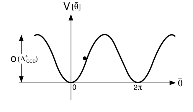
Figure 1: $V[\bar{\theta}]$ versus $\bar{\theta}$.

The maximum points of Fig. 1 gives $(2Z/(1+Z)^{2})f_{\pi}^{2}m_{\pi}^{2}$ from the current algebra estimate,[12] where $Z=m_{u}/m_{d}$ in terms of the current quark masses. Because $Z\sim\int[dA_{\mu}](\cdots)e^{i\bar{\theta}\int d^{4}x\{F\tilde{F}\}}$ and $\int d^{4}x\{F\tilde{F}\}={\rm integer}$, $\bar{\theta}$ is a periodic variable with periodicity of $2\pi$. Even though $V[\bar{\theta}]$ takes the above form, any $\bar{\theta}$ as shown with a dot in Fig. 1 will be allowed as any magnitude for the fine structure constant $\alpha_{em}$ is allowed theoretically. Thus, for a nonzero $\bar{\theta}$, CP invariance is violated in strong interactions. The axion solution for the strong CP problem is to identify $\bar{\theta}$ as a dynamical field $a$ instead of a coupling constant,

$$\bar{\theta}\ =\ {a\over F_{a}}.$$ (9)

If $\bar{\theta}$ is a coupling, different $\bar{\theta}$’s describe different worlds (or theories), but in the axion world different $\bar{\theta}$’s mean different vacua in the same theory. The vacuum is corresponding to $\bar{\theta}=0$ as depicted in Fig. 1.

An important feature to be satisfied in the axion models is that the axion $a$ does NOT have any potential except that coming from $\bar{\theta}\{F\tilde{F}\}$, or the mechanism does not work.

To make $\bar{\theta}$ dynamical, one must have a mechanism to introduce a scale $F_{a}$:(i) $a$ is the Goldstone boson of a spontaneously broken $U(1)_{A}$ symmetry where the $U(1)_{A}$ must have the QCD anomaly $\partial_{\mu}j^{\mu}\sim F\tilde{F}$ so that $(a/F_{a})F\tilde{F}$ coupling arises,[2] or
(ii) $a$ is a fundamental field in string models, and the scale $F_{a}$ arises from compactification. From low energy point of view the nonrenormalizable interaction term is present. The model-independent axion in string models belongs to this category,[13] or
(iii) $a$ is a composite field, and $F_{a}$ arises at the confining scale.[14]

Axion potential and cosmology

The invisible axion, due to its small couplings, has a dramatic cosmological consequence.[9] (A similar argument holds for the Polonyi problem.[15])

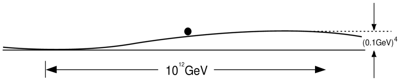
Figure 2: The almost flat axion potential.

In Fig. 2, we have shown the axion potential schematically. Actually, it is extremely flat as emphasized in Fig. 2 when the temperature of the universe $T$ is greater than 1 GeV. Only when the expansion rate of the universe is sufficiently slowed down at $H\simeq m_{a}$, the axion potential is felt and the vacuum starts to oscillate around $\bar{\theta}=0$. Since the axion lifetime is greater than $10^{20}$ times the age of the universe, the collective oscillation mode does not die out by the axion decay. Its amplitude of oscillation is shrunk only by the expansion of the universe, and corresponds to $\bar{\theta}\sim 10^{-20}$ now which is safely within the experimental upper bound.

For $V[a]\simeq(1/2)m_{a}^{2}a^{2}$, the energy density of axion $\rho=(1/2)\langle\dot{a}\rangle^{2}+V$ behaves like that of nonrelativistic particles. This is the reason that the axion is classified as the cold dark matter candidate, but it is only true for the classical motion. The cold axion energy density satisfies

$${d\over dt}\rho\ =\ -3H(\rho+p)$$ (10)

where $p=(1/2)\langle\dot{a}\rangle^{2}-V$. Parametrizing $\langle a\rangle$ as

$$\langle a(t)\rangle\ =\ A(t)\cos m_{a}t,$$ (11)

one obtains

$${d\over dt}(m_{a}A^{2})\ =\ -3H(m_{a}A^{2})\ \ \rightarrow\ \ {(m_{a}A^{2})_{f}\over(m_{a}A^{2})_{i}}\ =\ \left({R_{f}\over R_{i}}\right)^{-3}.$$ (12)

In the adiabatic expansion, the above equation shows that $m_{a}A^{2}$ is the number density, and hence the energy density becomes

$$\rho_{a}\ =\ m_{a}n_{a}\ =\ {1\over 2}m_{a}^{2}A^{2}.$$ (13)

The axion vacuum, denoted as a dot in Fig. 2 starts to roll down the hill when the temperature of the universe is lowered to $\sim$ 1 GeV. From then on the axion vacuum oscillate around the minimum $\bar{\theta}=0$. One can estimate the energy density of this collective motion of cold axions which is

$$\Omega_{a}\ =\ 2.1\times 10^{7}h^{-2}_{1/2}\left({{\rm GeV}\over T_{1}}\right)\left(T_{\gamma}\over 2.72\ {\rm K}\right)^{2}\left({A(T_{1})\over F_{a}}\right){F_{a}\over M_{Pl}}$$ (14)

where $h_{1/2}$ is the Hubble parameter in units of 50 $\rm km\cdot s^{-1}\cdot Mpc^{-1}$, $T_{1}\simeq 1$ GeV is the scale when axion vacuum starts to roll, and $A(T_{1})$ is the axion amplitude. From $\Omega_{a}\leq 1$, we obtain

$$F_{a}\ \leq\ 0.5\times 10^{12}h_{1/2}^{2}\ \rm GeV.$$ (15)

We also have $|\bar{\theta}|_{\rm now}<10^{-20}$.

2 Supersymmetric Extension

Last 20 years in theoretical particle physics is dominated by the study of supersymmetry which has been suggested as the best candidate toward the solution of the hierarchy problem. Therefore, axions should be understood in this framework if supersymmetry is the fundamental symmetry of nature. The starting point for phenomenology is the minimal supersymmetric standard model (MSSM) where all known particles of the standard model accompany their superpartners. In addition, two Higgs doublets and their superpartners are introduced : $H_{1}$ and $H_{2}$. $H_{1}$ couples to charged leptons and $d$-type quarks and $H_{2}$ couples to $u$-type quarks. In MSSM, all dimensionless couplings come from supersymmetric terms. For dimensionful parameters, there are two categories. There exists soft supersymmetry breaking parameters appearing in scalar mass terms and gaugino mass terms. These soft supersymmetry breaking parameters have magnitudes comparable to the gravitino mass

$$m_{3/2}\ \simeq\ {M_{I}^{2}\over M_{Pl}}.$$ (16)

For supersymmetry to be responsible for the hierarchy problem, $m_{3/2}\sim M_{W}$ and hence there must be an intermediate scale $M_{I}\simeq 10^{10}$ GeV $\sim$ $10^{11}$ GeV. Another dimensionful parameter in MSSM appears in the superpotential as the $\mu$ term

$$W_{\mu}\ =\ \mu H_{1}H_{2}.$$ (17)

This $\mu$ term is supersymmetric, and the intermediate scale $M_{I}$ is not directly related to $\mu$. Therefore, the parameter $\mu$ at Planck scale can be of order $M_{Pl}$. Then, the electroweak scale $M_{W}$ cannot be generated. On the other hand, the magnitude of $\mu$ is known to be nonzero from high energy experiments. In addition, if it were zero, one expects an electroweak scale axion which has been ruled out phenomenologically.[6] Also, $\langle H_{1}\rangle=0$ results from $\mu=0$, which is in contradiction with making $Q=-1/3$ quarks massive. Therefore, $\mu$ is expected to be of order electroweak scale $\sim m_{3/2}$. How $\mu\sim M_{W}$ can occur is the so-called $\mu$ problem.[16]

If one introduces a Peccei-Quinn symmetry in supergravity, one can generate a reasonable $\mu$ term. For example, a nonrenormalizable term

$$W_{\mu}\ =\ {1\over M_{Pl}}S_{1}S_{2}H_{1}H_{2}$$ (18)

can be considered. Here $S_{1,2}$ are gauge singlets. Because of the Peccei-Quinn symmetry, one assigns charge 1 to $H_{1}$ and $H_{2}$ fields. Then the sum of the $S_{1}$ and $S_{2}$ charges must be -2. Therefore, by giving nonzero vacuum expectation values to $S_{1}$ and $S_{2}$ at $\sim 10^{12}$ GeV, one breaks the Peccei-Quinn symmetry and generate a correct order for the $\mu$ term. In the process, there results an invisible axion.

A general K$\ddot{\rm a}$hler potential is restricted by the reality condition only.[17] Therefore, one can write

$${\cal G}\ =\ \sum_{a}y^{a}y^{\dagger a}+zz^{\dagger}+(\lambda H_{1}H_{2}+\rm h.c.)=\cdots$$ (19)

with observable sector fields $y^{a}$ and a hidden sector field $z$. Of course, such $H_{1}H_{2}$ term can be present in the K$\ddot{\rm a}$hler potential, but one has to explain why $M_{Pl}H_{1}H_{2}$ is not present in the superpotential. This can be done only by a symmetry argument.[18]

3 Superstring Axion

The N=1 supergravity theory in D=10 needs a supergravity multiplet

$$B_{MN}\ \ (M,N=0,1,\cdots,9);\ \ \ \ M,N\ \rm antisymmetric.$$ (20)

The D=10 supergravity models obtained from superstring models also needs the $B_{MN}$ field. After compactifying 6 internal dimensions, the field strength of $B_{\mu\nu}\ (\mu,\nu,\rho=0,1,2,3)$ is sometimes duality transformed to see its physical implications,

$$H_{\mu\nu\rho}\ =\ 16\pi^{2}\epsilon_{\mu\nu\rho\sigma}J_{1}^{\sigma}$$ (21)

where $J_{1}^{\sigma}$ is a gauge invariant d=4 axial vector current,

$$\partial_{\mu}J_{1}^{\mu}\ =\ {1\over 32\pi^{2}}\left({\rm Tr}\ R_{\mu\nu}\tilde{R}^{\mu\nu}-{1\over 30}{\rm Tr}\ F_{\mu\nu}\tilde{F}^{\mu\nu}\right).$$ (22)

We define the model-independent axion $a_{MI}$ as the linear combination of $a_{1}$

$$F_{1}\partial^{\mu}a_{1}=J_{1}^{\mu}={1\over 96\pi^{2}}\epsilon^{\mu\nu\rho\sigma}H_{\nu\rho\sigma}$$ (23)

and $B_{mn}\equiv B_{A}$ obtained from the process of compactification,

$${\cal L}_{eff}\ =\ {1\over 2}(\partial_{\mu}a_{1})^{2}+{1\over 2}\sum_{A=1}^{N}(\partial_{\mu}B_{A})^{2}-{a_{1}\over 32\pi^{2}F_{1}}{1\over 30}F\tilde{F}$$

$$-{1\over 32\pi^{2}F_{2}}(\sum_{A}\Gamma^{A}B_{A})({1\over 30}\sum_{a}C^{a}{\rm Tr}_{a}F\tilde{F})$$

where $\Gamma^{A}$ and $C^{a}$ depend on compactification. Note that $F_{1}$ can be estimated by comparing with Newton’s constant [19]

$$F_{1}\ =\ {g^{2}\over 192\pi^{5/2}}M_{Pl}\ \simeq\ 1.5\times 10^{15}\ \rm GeV.$$ (24)

Actually, due to the $F_{2}$ term the model-independent axion decay constant $F_{a}$ is not exactly $F_{1}$. $F_{1}$ gives an idea on the magnitude of $F_{a}$. For example, the $E_{8}\times E^{\prime}_{8}$ heterotic string compactified with $b_{2,0}=b_{0,2}=0,b_{1,1}=1$ leads to the following coupling [20]

$${1\over 32\pi^{2}F_{1}}a_{1}(F\tilde{F}+F^{\prime}\tilde{F}^{\prime})+{1\over 32\pi^{2}F_{2}}a_{2}(F\tilde{F}-F^{\prime}\tilde{F}^{\prime})$$ (25)

from which we obtain

$$F_{a}\ =\ {1\over 2}\sqrt{F_{1}^{2}+F_{2}^{2}}\ >\ 0.7\times 10^{15}\ \rm GeV.$$ (26)

In general, the model-independent axion scale falls in the compactification scale $\sim 10^{17}$ GeV. Therefore, the scale of $a_{MI}$ is too large: the universe collapses before life was born if there is no extra confining gauge group, or the strong CP problem is not solved by $a_{MI}$ if there exists an extra hidden sector confining gauge group. Thus it is very important to find a solution of the strong CP problem in string models.

Many compactification schemes introduce an anomalous $U(1)$ gauge symmetry.[21] This anomalous $U(1)$ has been used to break extra $U(1)$ gauge symmetries appearing in many 4D string models. The anomaly is not troublesome in string models due to the model-independent axion $a_{MI}$ which makes the $U(1)$ gauge boson massive by becoming its longitudinal degree. Thus we see that the old ’t Hooft mechanism is operative here,

$$a_{MI}\ (nonlinearly\ realized\ global\ symmetry)+anomalous\ U(1)\ gauge\ symmetry$$

$$\rightarrow U(1)\ global\ symmetry$$

Comparing the Lagrangians of spontaneously broken $U(1)$ gauge theory

$${\cal L}\ =\ D_{\mu}\phi^{*}D^{\mu}\phi\ =\ {1\over 2}(\partial_{\mu}a)^{2}-evA_{\mu}\partial^{\mu}a$$ (27)

and the anomalous $U(1)$ gauge theory with $a_{MI}$

$${\cal L}\ =\ -{1\over 4}F^{2}+{1\over 2}(\partial_{\mu}a_{MI})^{2}+mA_{\mu}\partial^{\mu}a_{MI}+\cdots,$$ (28)

we obtain $M_{A}^{2}=m^{2}$. Below the compactification scale $m$, the gauge boson $A_{\mu}$ is decoupled and a global $U(1)$ symmetry is present. Therefore, if there is no extra confining gauge group, the axion decay constant can be lowered due to this new global symmetry which acts as an anomalous $U(1)$ Peccei-Quinn symmetry.[22] However, a popular scenario for supersymmetry breaking is to introduce an extra confining gauge group at $\sim 10^{13}$ GeV scale, the quantum hidden sector dynamics (QHD). In this case, the global symmetry produced by the ’t Hooft mechanism is explicitly broken by the quantum effects of QHD and we lack the axion needed to settle $\bar{\theta}$ at zero. To solve the strong CP problem, one assumes an approximate global symmetry in this case.[23]

Before discussing the axino-gravitino cosmology, consider

$${\rm Standard\ Model}\otimes SU(N)_{\rm hidden\ sector}.$$ (29)

The model-independent axion $a_{MI}$ has the following potential

$$V[a_{MI}]\ =\ \Lambda^{4}_{QCD}(1-\cos\bar{\theta})+\epsilon\Lambda^{4}_{h}(1-\cos\theta^{\prime})$$ (30)

where $\bar{\theta}\equiv(a_{MI}/F_{a})+\theta_{QFD}$ and $\theta^{\prime}\equiv a_{MI}/F_{a}$. Because the QHD scale $\Lambda_{h}\gg\Lambda_{QCD}$, $\bar{\theta}$ is not settled at 0. But if $\epsilon=0$, the $\Lambda^{4}_{QCD}$ term dominates and $\bar{\theta}=0$ is the minimum of the potential. Therefore,if a sufficiently small $\epsilon$ (of order $<10^{-9}$) can be found, and then the model is allowed. One obvious solution toward negligible $\epsilon$ is to introduce a massless QHD quark. The difficulty of introducing a massless QHD quark is to introduce another global symmetry, not related to the $a_{MI}$, in string models. Thus the strong CP problem in superstring models does not have an obvious solution with $\epsilon=0$ yet. But there exists a possibility of having a very small $\epsilon$ from the consideration of supersymmetry and a global $U(1)$ resulting from the anomalous gauge $U(1)$.[24]

4 Axino-gravitino Cosmology

Axion models in supergravity theories necessarily introduce the gravitino $\tilde{G}$ and the axino $\tilde{a}$ whose masses we denote as $m_{3/2}$ and $m_{\tilde{a}}$, respectively. Of course, the scalar partner of $\tilde{a}$ is present and it is sometimes called saxion $s$.[25] The saxion mass is of order $m_{3/2}$. Before discussing the axino-gravitino cosmology, let us briefly comment some aspects of the gravitino mass effect on cosmology.

For $m_{3/2}\geq 1$ TeV, this region of the gravitino mass is obtained from the ⁴He abundance calculation so that the nucleosynthesis must starts from the scratch after the reheating by gravitino decay.[27] The gravitino lifetime is extremely long,

$$\tau(m_{\tilde{\gamma},gluino}\ll m_{3/2})\ \simeq\ 4.4\times 10^{7}\ {\rm s}\ \left({100\ {\rm GeV}\over m_{3/2}}\right)^{3}$$ (31)

which is the reason that the gravitino is important in cosmology.

For 20 GeV $<\ m_{3/2}\ <$ 1 TeV, the gravitino decayed sometime between the epochs of nucleosynthesis and recombination. Even if one inflates away the primodial gravitinos, $\tilde{G}$ would have been produced thermally. If these thermally produced gravitinos were too abundant, they would have destroyed the precious deuterium. This consideration restricts that the reheating temperature after gravitino decay must be bounded[28]

$$T_{R,max}\ \simeq\ 10^{11}\sqrt{{m_{3/2}\over 100\ \rm GeV}}\ {\rm GeV}.$$ (32)

The above bound is obtained by considering the scattering cross section at zero temperature. In cosmology, however, high temperature effect may be important, since plasma of particles does not respect supersymmetry. But a definite conclusion on this topic is premature.[29]

In addition, saxion $s$ affects the evolution of the universe by injecting more particles when it decays. In this case, the bound on the axion decay constant $F_{a}$ can be raised a bit.[26]

Gravitino mass in the eV range

Finally, let us discuss the axino-gravitino cosmology. So far, we discussed supergravity models with a hidden sector confining force, $\Lambda_{h}\sim 10^{13}$ GeV, which is the source of supersymmetry breaking. However, if supersymmetry is broken by supercolor at $\Lambda_{supercolor}\simeq 1\sim 10^{3}$ TeV,[30] i.e. with $m_{3/2}\simeq 0.4\times 10^{-3}\ {\rm eV}\ \sim\ 0.4\ {\rm keV}$, then axino $\tilde{a}$ can decay to gravitino $\tilde{G}$ plus axion,

$$\tilde{a}\rightarrow\tilde{G}+a.$$ (33)

This process might be very important in cosmology since the lifetime of the axino is falling in the cosmologically interesting region. Actually, this kind belongs to the cosmological scenario with late decaying particles. Cosmology with late decaying particles was considered first by Bardeen, Bond and Efstathiou in 1987,[31] and the now-dead 17 keV neutrino was used to realize this scenario. After the finding that CDM models are in trouble with the COBE data of large scale structure of the universe, Chun, Kim and Kim [32] first considered the axino-gravitino cosmology, not knowing the old work of Bardeen et al.[31] Recently, the late decaying particle cosmology is studied by many groups primarily using one of the neutrinos as the late decaying particle.[33]

In the axino-gravitino cosmology, the axino lifetime is estimated to be[26]

$$\tau_{\tilde{a}}\ =\ {96\pi M^{2}m_{3/2}^{2}\over m_{\tilde{a}}^{5}}\ =\ 1.2\times 10^{12}\ {\rm s}\ \left({{\rm MeV}\over M_{\tilde{a}}}\right)^{5}\left({m_{3/2}\over\rm eV}\right)^{2}$$ (34)

from the Lagrangian ${\cal L}=(1/M)\bar{\psi}_{\mu}\gamma^{\nu}\partial_{\nu}z^{*}\gamma^{\mu}\tilde{a}$ where $M=M_{Pl}/8\pi$. The axino decoupling temperature is calculated mainly from the process $q+\bar{q}\leftrightarrow\tilde{a}+\tilde{g}$,[25]

$$T_{\tilde{a}D}\ \simeq\ 10^{11}\ {\rm GeV}\ \left({F_{a}\over 10^{12}\ {\rm GeV}}\right)^{2}\left({0.1\over\alpha_{c}}\right)^{3}.$$ (35)

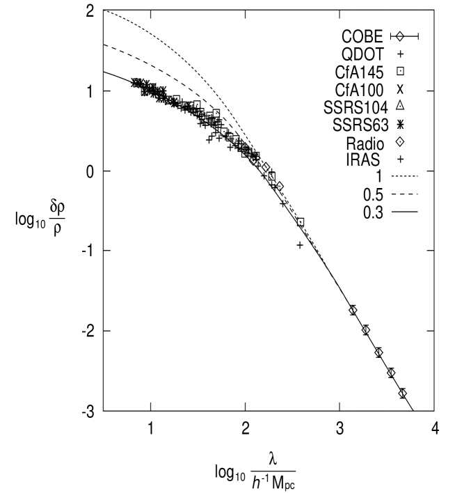
Figure 3: log${}_{10}(\delta\rho/\rho)$ versus log${}_{10}(\lambda/h^{-1}{\rm Mpc})$. The solid line corresponds to the $\Omega h=0.3$ CDM model, while the dashed and dotted lines corresponds to the $\Omega h=0.5$ and 1 CDM models, respectively.

Dark matter and structure formation

We envision that cold axions remain as dark matter, and gravitinos and hot axions produced by the axino decay remain as hot dark matter. Therefore, this late decaying particles with cold axions can mimick the mixed dark matter model.[34] The cold dark matter (CDM) model was successful in 80’s. But the normalization determined by the COBE data necessiated modifications of the CDM models. The study of large scale structure is greatly simplified if we use the evolved fluctuation spectrum calculated by Davis et al,[35]

$$|\delta^{2}_{k}|^{2}\ =\ {Ak\over(1+\alpha k+\beta k^{3/2}+\gamma k^{2})^{2}}$$ (36)

where $\alpha=1.7\ell,\beta=9.0\ell,\gamma=1.0\ell$ with

$$\ell\ =\ (\Omega h^{2})^{-1}\theta^{1/2}\rm Mpc.$$ (37)

Here, $\theta$ is determined by relativistic particles and the old CDM model corresponds to $\theta=1$. In Fig. 3, we present several CDM models with different values of $\Omega h$.

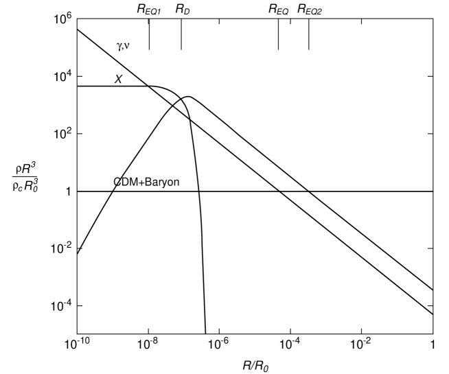
Figure 4: Scale factor versus energy densities of radiation $(\gamma,\nu)$, axino ($\tilde{a}$), decay products of axino ($\tilde{G},a$) and cold axion ($\langle a\rangle$) for $m_{\tilde{a}}=10$ MeV, $m_{3/2}=76$ meV and $\rho_{\langle a\rangle 0}=\rho_{c}$.

Successful fits corresponds to

(i) $\Omega_{\rm cosmological\ constant}\simeq 0.8,\ \Omega_{CDM}\simeq 0.2$, or
(ii) $\Omega_{CDM}\simeq 0.7,\ \Omega_{HDM}\simeq 0.3$, or
(iii) $\Omega_{CDM}=0.2\sim 0.3$, or
(iv) Large biasing or antibiasing, or
(v) Initial fluctuation spectrum with less power at small scales.

Note that the effect of Case (iii) can be mimicked if we build a model with $\theta\neq 1$ but with $\Omega=1$. It is in effect a CDM plus HDM model since $\theta\neq 1$ needs hot dark matter except photons and neutrinos. Instead of $\ell$, let us define

$$\lambda_{EQ}\ \simeq\ 30(\Omega h^{2})^{-1}\theta^{1/2}\rm Mpc$$ (38)

where

$$\theta\ =\ {\rho({\rm relativistic\ particles})\over 1.68\rho_{\gamma}}.$$ (39)

Here, the denominator corresponds to neutrinos plus photons and the numerator corresponds to all hot matters at present. A larger $\theta$ or a larger $\lambda_{EQ}$ with $\Omega=1$, which is required in most inflationary models, can give the same $\ell$ given by Case (iii). Case (iii) with $\Omega\neq 1$, even though it gives a correct large scale structure, is not welcome in inflationary models. Thus a late decaying particle scenario mimicking Case (iii) with $\Omega h_{1/2}=1$ and $\theta=1.8$ is more welcome in inflationary models. In Fig. 4 we present $\rho$ versus $R$ (the scale factor) plot. From this figure, we note that for $R>R_{EQ2}$ the universe is matter dominated and galaxies are formed. However, we also note that between $R_{EQ1}$ and $R_{D}$ (corresponding to the time of axino decay) there is another epoch of matter domination. The large scale structures corresponding to this epoch is the size of globular clusters. It will be interesting if this turns out to be true.

In Fig. 5 we present the allowed regions of $m_{3/2}$ and $m_{\tilde{a}}$, obtained from various cosmological data. The axino-gravitino cosmology giving a desirable large scale structures discussed above is denoted as a heavy dotted line.

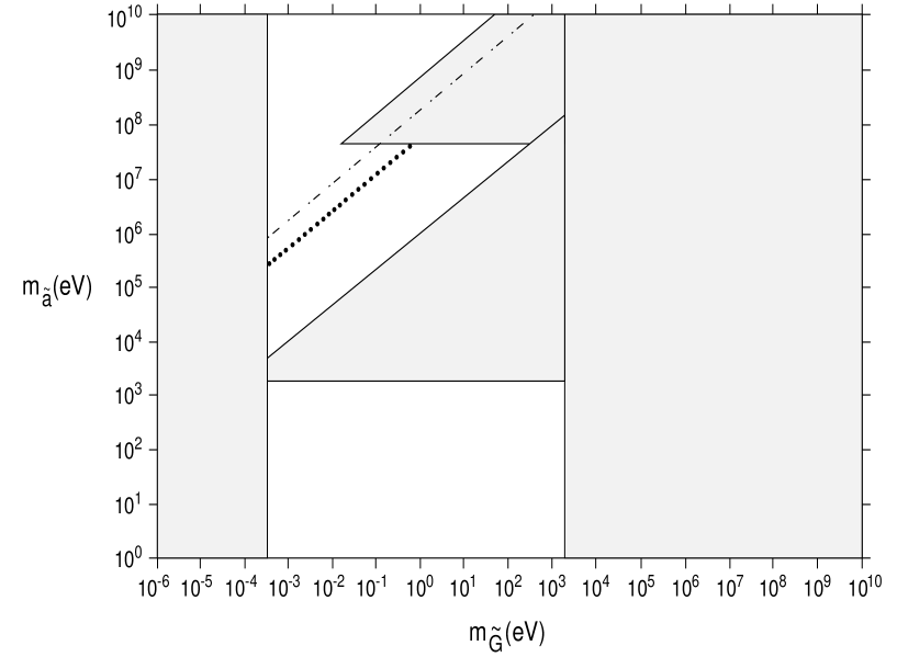
Figure 5: Allowed region in axino mass–gravitino mass. Grey regions are excluded by the closure bound and the nucleosynthesis bound. Successful fit to COBE data corresponds to the heavy dotted line.

5 Conclusion

The $\theta_{QCD}$ parameter problem of the standard model leads to an axionic extension of the standard model. Thus, one can consider the invisible axion $a$ in addition to the standard model particles. From the data on SN1987A and cosmological energy density we have an axion widow $10^{10}\sim 10^{12}$ GeV. It is possible to introduce this range of $F_{a}$ in gauge models without supersymmetry. In supersymmetric models, one has the $\mu$ term which can be introduced by a spontaneously broken Peccei-Quinn symmetry. In superstring models, the invisible axion satisfying the experimental bound is more difficult to introduce. Without an extra confining force, the model-independent axion $a_{MI}$ can be made as the conventional invisible axion with $F_{a}\simeq 10^{12}$ GeV at low energy in models with an anomalous $U(1)$ gauge group. With an extra nonabelian gauge group, it is more difficult to make the model-independent axion the conventional invisible axion. Finally, we commented the interesting cosmological scenario if the gravitino mass falls in the eV range, which is the first explicit example of cosmology with late decaying particles after the COBE data.

References

- [1] H. Georgi, H. R. Quinn and S. Weinberg, Phys. Rev. Lett. 33, 451 (1974); J. Pati and Abdus Salam, Phys. Rev. D10, 275 (1974); H. Georgi and S. L. Glashow, Phys. Rev. Lett. 32, 438 (1974).
- [2] R. D. Peccei and H. R. Quinn, Phys. Rev. D16, 1791 (1977); S. Weinberg, Phys. Rev. Lett. 40, 223 (1978); F. Wilczek, Phys. Rev. Lett. 40, 279 (1978); J. E. Kim, Phys. Rev. Lett. 43, 103 (1979); A. P. Zhitnitskii, Sov. J. Nucl. Phys. 31, 260 (1980); M. A. Shifman, V. I. Vainstein and V. I. Zakharov, Nucl. Phys. B166, 4933 (1980); M. Dine, W. Fischler and M. Srednicki, Phys. Lett. B104, 199 (1981).
- [3] S. Weinberg, Phys. Rev. D19, 1277 (1979); L. Susskind, Phys. Rev. D20, 2619 (1979).
- [4] E. Witten, Nucl. Phys. B188, 513 (1981).
- [5] See, for example, L. Ibanez and G. Ross, Phys. Lett. B332, 110 (1994).
- [6] J. E. Kim, Phys. Rep. 150, 1 (1987); H.Y. Cheng, Phys. Rep. 158, 1 (1988); R. D. Peccei, in CP Violation, ed. C. Jarlskog (World Scientific, Singapore, 1989).
- [7] A. A. Belavin, A. Polyakov, A. Schwartz, and Y. Tyupkin, Phys. Lett. B59, 85 (1974).
- [8] I. S. Altarev et al, Phys. Lett. B276, 242 (1992).
- [9] J. Preskill, M. B. Wise and F. Wilczek, Phys. Lett. B120, 127 (1983); L. F. Abbott and P. Sikivie, Phys. Lett. B120, 133 (1983); M. Dine and W. Fischler, Phys. Lett. B120, 137 (1983).
- [10] D. B. Kaplan and A. Manohar, Phys. Rev. Lett. 56, 2004 (1986); K. Choi, C. W. Kim and W. K. Sze, Phys. Rev. Lett. 61, 794 (1988); K. Choi, Nucl. Phys. B383, 58 (1992).
- [11] C. Vafa and E. Witten, Phys. Rev. Lett. 53, 535 (1984).
- [12] W. A. Bardeen and S.-H. H. Tye, Phys. Lett. B74, 229 (1978); V. Baluni, Phys. Rev. D19, 2227 (1979).
- [13] E. Witten, Phys. Lett. 149, 351 (1984).
- [14] J. E. Kim, Phys. Rev. D31, 1733 (1985), K. Choi and J. E. Kim, Phys. Rev. D32, 1828 (1985).
- [15] G. D. Coughlan, W. Fischler, E. W. Kolb, S. Raby and G. G. Ross, Phys. Lett. B131, 59 (1983).
- [16] J. E. Kim and H. P. Nilles, Phys. Lett. B138, 150 (1984).
- [17] G. F. Giudice and A. Masiero, Phys. Lett. B206, 480 (1988); I. Antoniadis, E. Gava, K. S. Narain and T. R. Taylor, Nucl. Phys. B432, 187 (1994).
- [18] J. E. Kim and H. P. Nilles, Mod. Phys. Lett. A9, 3575 (1994).
- [19] K. Choi and J. E. Kim, Phys. Lett. B154, 393 (1985).
- [20] K. Choi and J. E. Kim, Phys. Lett. B164, 71 (1985).
- [21] M. Dine, N. Seiberg and E. Witten, Nucl. Phys. B289, 317 (1987); J. J. Atick, L. J. Dixon and A. Sen, Nucl. Phys. B292, 109 (1987); M. Dine, I. Ichinose and N. Seiberg, Nucl. Phys. B293, 253 (1987); A. Font, L. E. Ibanez, H. P. Nilles and F. Quevedo, Nucl. Phys. B307, 109 (1988); J. A. Casas, E. K. Katehou and C. Munoz, Nucl. Phys. B317, 171 (1989).
- [22] J. E. Kim, Phys. Lett. B207, 434 (1988).
- [23] E. J. Chun, J. E. Kim and H. P. Nilles, Nucl. Phys. B370, 105 (1992).
- [24] J. E. Kim, to be published.
- [25] K. Rajagopal, M. S. Turner and F. Wilczek, Nucl. Phys. B358, 447 (1991).
- [26] J. E. Kim, Phys. Rev. Lett. 67, 3465 (1991).
- [27] S. Weinberg, Phys. Rev. Lett. 48, 1303 (1982).
- [28] J. Ellis, J. E. Kim and D. V. Nanopoulos, Phys. Lett. B145, 181 (1984). For a recent study, see, M. Kawasaki and T. Moroi, Prog. Theo. Phys. 93, 879 (1995); T. Moroi, Thesis (1995) hep-ph/9503210.
- [29] W. Fischler, Phys. Lett. B332, 227 (1994); R. G. Leigh and R. Rattazzi, Phys. Lett. B352, 20 (1995); H. Fujisaki, K. Kumekawa, M. Yamaguchi and M. Yoshimura, hep-ph/9511381.
- [30] M. Dine and A. E. Nelson, Phys. Rev. D48, 1277 (1993).
- [31] J. Bardeen, J. R. Bond, and G. Efstathiou, Astro. Phys. J. 321, 28 (1987).
- [32] E. J. Chun, H. B. Kim and J. E. Kim, Phys. Rev. Lett. 72, 1956 (1994); H. B. Kim and J. E. Kim, Nucl. Phys. B433, 421 (1995).
- [33] M. S. Turner, Phys. Rev. Lett. 72, 3754 (1994); R. N. Mohapatra and A. Riotto, Phys. Rev. Lett. 73, 1324 (1994); A. D. Dolgov, S. Pastor and J. W. F. Valle, preprint astro-ph/9506011.
- [34] E. L. Wright et al., Astrophys. J. 396, L13 (1992).
- [35] M. Davis, G. Efstathiou, C. S. Frenk, and S. D. M. White, Nature 356, 489 (1992).