Kiss Lajos bácsi, a Fizika Tanára emlékére hep-ph/9511404

Dedicated to the memory of L. Kiss, Teacher of Physics

BOSE-EINSTEIN CORRELATIONS FOR JETS AND

HEAVY ION REACTIONS

T. CSÖRGŐ

Department of Physics, Columbia University, 538 West 120th, New York, NY 10027

MTA KFKI RMKI, H – 1525 Budapest 114, POB 49, Hungary

E-mail: csorgo@sgiserv.rmki.kfki.hu

and

B. LÖRSTAD

Physics Institute, University of Lund, Professorsgatan 1, S – 223 63 Lund, Sweden

E-mail: bengt@quark.lu.se

ABSTRACT

Bose-Einstein correlations and invariant momentum distributions are analyzed for longitudinally expanding finite systems, like jets in elementary particle collisions or systems created in high energy heavy ion reactions.

1 Introduction

Bose-Einstein correlations are in general not measuring the whole geometrical sizes of big and expanding finite systems^?,?,? since the expansion may result in strong correlations between space-time and momentum space variables not only in the longitudinal, but in the transverse and temporal directions, too^?.

Where have all the geometrical sizes gone? One can show^?,?, that they are disguised in the invariant momentum distribution of the bosons in case they cancel from the radius parameters of the Bose-Einstein correlation function (BECF).

We shall briefly review herewith the results presented in refs.^?,?,?,? which shall be appended with an application to jet size determination.

2 Wigner Function Formalism

The two-particle inclusive correlation function is defined and approximately expressed in the Wigner function formalism as

$$C(\Delta k;K) = {\displaystyle\langle n(n-1)\rangle\over\displaystyle\langle n\rangle^{2}}{\displaystyle N_{2}({\bf p}_{1},{\bf p}_{2})\over\displaystyle N_{1}({\bf p}_{1})\,N_{1}({\bf p}_{2})}\simeq 1+{\displaystyle\mid\tilde{S}(\Delta k,K)\mid^{2}\over\displaystyle\mid\tilde{S}(0,K)\mid^{2}}.$$ (1)

In the above line, the Wigner-function formalism^?,?,? is utilized assuming fully chaotic (thermalized) particle emission. The covariant Wigner-transform of the source density matrix, $S(x,p)$ is a quantum-mechanical analogue of the classical probability that a boson is produced at a given $x^{\mu}=(t,{\bf r})=(t,r_{x},r_{y},r_{z})$ with $p^{\mu}=(E,{\bf p})=(E,p_{x},p_{y},p_{z})$. The auxiliary quantity $\tilde{S}(\Delta k,K)=\int d^{4}xS(x,K)\exp(i\Delta k\cdot x)$ appears in the definition of the BECF, with $\Delta k=p_{1}-p_{2}$ and $K={(p_{1}+p_{2})/2}$. The single- and two-particle inclusive momentum distributions (IMD-s) are given by

$$N_{1}({\bf p})={\displaystyle E\over\sigma_{tot}}{\displaystyle d\sigma\over\displaystyle d{\bf p}}=\tilde{S}(\Delta k=0,p),\quad \quad N_{2}({\bf p_{1}},{\bf p_{2}})={\displaystyle E_{1}E_{2}\over\sigma_{tot}}{\displaystyle d\sigma\over\displaystyle d{\bf p}_{1}\,d{\bf p}_{2}},$$ and (2)

where $\sigma_{tot}$ is the total inelastic cross-section. Note that in this work we utilize the following normalization of the emission function^?: $\int{\displaystyle d^{3}{\bf p}\over\displaystyle E}d^{4}xS(x,p)=\langle n\rangle$.

3 Effects from Large Halo of Long-Lived Resonances

If the bosons originate from a core which is surrounded by a halo of long-lived resonances, the IMD and the BECF can be calculated in a straightforward manner. The detailed description is given in ref.^?, here we review only the basic idea.

If the emission function can be approximately divided into two parts, representing the core and the halo, $S(x;K)=S_{c}(x;K)+S_{h}(x;K)$ and if the halo is characterized by large length-scales so that $\tilde{S}_{h}(Q_{min};K)$ $<<\tilde{S}_{c}(Q_{min};K)$ at a finite experimental resolution of $Q_{min}\geq 10$ MeV, then the IMD and the BECF reads as

$$N_{1}({\bf p}) = N_{1,c}({\bf p})+N_{1,h}({\bf p}),$$ (3)

$$C(\Delta k;K) = 1+\lambda_{*}{\displaystyle\mid\tilde{S}_{c}(\Delta k,K)\mid^{2}\over\displaystyle\mid\tilde{S}_{c}(0,K)\mid^{2}},$$ (4)

where $N_{1,i}({\bf p})$ stands for the IMD of the halo or core for $i=h,c$ and

$$\lambda_{*} = \lambda_{*}(K=p)=\left[{\displaystyle N_{1,c}({\bf p})\over\displaystyle N_{1}({\bf p})}\right]^{2}.$$ (5)

Thus within the core/halo picture the phenomenological $\lambda_{*}$ parameter can be obtained in a natural manner at a given finite resolution of the relative momentum. This parameter has been introduced to the literature by Deutschmann long time ago^?. In the core/halo picture, the effective or measured intercept parameter $\lambda({\bf p})$ can be interpreted as the momentum dependent square of the ratio of the IMD of the core to the IMD of all particles emitted.

4 General Considerations and Results

We are considering jets in elementary particle reactions or high energy heavy ion reactions, which correspond to systems undergoing an approximately boost-invariant longitudinal expansion. For fully boost-invariant longitudinal expansions, the emission function may depend on boost-invariant variables only. These are defined as $\tau=\sqrt{t^{2}-r_{z}^{2}},\,$ $\eta=0.5\ln[(t+z)\,/\,(t-z)],\,$ $m_{t}=\sqrt{E^{2}-p_{z}^{2}},\,$ $y=0.5\ln[(E+p_{z})\,/\,(E-p_{z})]\,$ and $r_{t}=\sqrt{r_{x}^{2}+r_{y}^{2}}$. For finite systems, the emission function may depend on $\eta-y_{0}$ too, where $y_{0}$ stands for the mid-rapidity. Approximate boost-invariance is recovered in the $\mid\eta-y_{0}\mid<<\Delta y$ region, where the width of the rapidity distribution is denoted by $\Delta y$. In terms of these variables the emission function can be rewritten as

$$S_{c}(x;K)\,d^{4}x = S_{c,*}(\tau,\eta,r_{x},r_{y})\,d\tau\,\tau_{0}d\eta\,dr_{x}\,dr_{y}.$$ (6)

The subscript _∗ indicates that the functional form of the source function is changed, and it stands for a dependence on $K$ and $y_{0}$ also.

In the standard HBT coordinate system^?, the mean and the relative momenta are $K=(K_{0},K_{{out}},0,K_{L})$ and $\Delta k=(Q_{0},Q_{{out}},Q_{side},Q_{L})$. Note that the _side component of the mean momentum vanishes by definition^?,?. Since the particles are on mass-shell, we have $0=K\cdot\Delta k=K_{0}Q_{0}-K_{L}Q_{L}-K_{{out}}Q_{{out}}.$

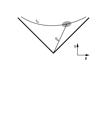
Figure 1: Emission of particles with a given momentum is centered around $\tau_{s}$ and $\eta_{s}$ for systems undergoing boost-invariant longitudinal expansion, as indicated by the shaded area.

Introducing $\beta_{L}=K_{L}/K_{0}$ and $\beta_{out}=K_{out}/K_{0}$, the energy difference $Q_{0}$ can thus be expressed as

$$Q_{0} = \beta_{L}Q_{L}+\beta_{{out}}Q_{out}.$$ (7)

If the emission function has a such a structure that it is concentrated in a narrow region around $(\tau_{s},\eta_{s})$ in the $(\tau,\eta)$ plane, then one can evaluate the BECF in terms of variables $\tau$ and $\eta$ by utilizing the expansion

$$\Delta k\cdot x = Q_{0}t-Q_{out}r_{x}-Q_{side}r_{y}-Q_{L}r_{z}\simeq$$ (9)

$$Q_{\tau}{\tau}-Q_{out}r_{x}-Q_{side}r_{y}-Q_{\eta}{\tau}_{s}(\eta-\eta_{s}).$$

The coefficients of the ${\tau}$ and the ${\tau}_{s}({\eta}-{\eta}_{s})$ are new variables given by

$$Q_{\tau} = Q_{0}\cosh[\eta_{s}]-Q_{L}\sinh[\eta_{s}]=(\beta_{t}Q_{out}+\beta_{L}Q_{L})\cosh[\eta_{s}]-Q_{L}\sinh[\eta_{s}],$$ (10)

$$Q_{\eta} = Q_{L}\cosh[\eta_{s}]-Q_{0}\sinh[\eta_{s}]=Q_{L}\cosh[\eta_{s}]-(\beta_{t}Q_{out}+\beta_{L}Q_{L})\sinh[\eta_{s}].$$ (11)

In terms of these new variables the BECF reads as

$$C(\Delta k;K)\simeq 1+{\displaystyle\mid\tilde{S}(\Delta k,K)\mid^{2}\over\displaystyle\mid\tilde{S}(0,K)\mid^{2}}\simeq 1+\lambda_{*}(K){\displaystyle\mid\tilde{S}_{c,*}(Q_{\tau},Q_{\eta},Q_{out},Q_{side})\mid^{2}\over\displaystyle\mid\tilde{S}_{c,*}(0,0,0,0)\mid^{2}}.$$ (12)

At this level, the shape of the BECF can be rather complicated, it may have non-Gaussian, non-factorizable structure. Gaussian approximation to eq. (12) may break down as discussed in more detail in the Appendix of ref.^?.

5 Mixing Angle for HBT

In the experimental analysis, one of the most frequently^? but not exclusively^? applied parameterization of the BECF is some version of a Gaussian approximation. The out-longitudinal cross-term of BECF has also been discovered in this context recently^?. In order to identify how this term may come about, let us assume that

$$S_{c,*}(\tau,\eta,r_{x},r_{y}) = H_{*}({\tau})\,G_{*}({\eta})\,I_{*}(r_{x},r_{y}).$$ (13)

In Gaussian approximation one also assumes that

$$H_{*}(\tau) \propto \exp(-({\tau}-{\tau}_{s})^{2}/(2\Delta{\tau}_{*}^{2})\,),$$ (14)

$$G_{*}(\eta) \propto \exp(-(\eta-\eta_{s})^{2}/(2\Delta{\eta}_{*}^{2})\,),$$ (15)

$$I_{*}(r_{x},r_{y}) \propto \exp(-(\,(r_{x}-r_{x,s})^{2}+(r_{y}-r_{y,s})^{2})/(2R_{*}^{2})\,).$$ (16)

The corresponding BECF is given by a diagonal form as

$$C(\Delta k;K)=1+\lambda_{*}\,\exp(-Q_{\tau}^{2}\Delta\tau_{*}^{2}-Q_{\eta}^{2}{\tau}_{s}^{2}\Delta{\eta}_{*}^{2}-Q_{t}^{2}R_{*}^{2}).$$ (17)

This diagonal form shall be transformed to an off-diagonal one if one introduces the kinematic relations between the variables $Q_{\tau},Q_{\eta}$ and the variables $Q_{out},Q_{L}$. In the HBT coordinate system^? one finds

$$C(\Delta k;K) = 1+\lambda_{*}\exp(-R_{side}^{2}Q_{side}^{2}-R_{out}^{2}Q_{out}^{2}-R_{L}^{2}Q_{L}^{2}-2R^{2}_{{out},L}Q_{out}Q_{L}),$$ (18)

$$R_{side}^{2} = R_{*}^{2},$$ (19)

$$R_{out}^{2} = R_{*}^{2}+\delta R_{out}^{2},$$ (20)

$$\delta R_{out}^{2} = \beta_{t}^{2}(\cosh^{2}[{\eta}_{s}]\Delta{\tau}_{*}^{2}+\sinh^{2}[{\eta}_{s}]{\tau}_{s}^{2}\Delta{\eta}_{*}^{2}),$$ (21)

$$R_{L}^{2} = (\beta_{L}\sinh[\eta_{s}]-\cosh[{\eta}_{s}])^{2}{\tau}_{s}^{2}\Delta{\eta}_{*}^{2}+(\beta_{L}\cosh[\eta_{s}]-\sinh[{\eta}_{s}])^{2}\Delta{\tau}_{*}^{2},$$ (22)

$$R_{{out},L}^{2} = (\beta_{t}\cosh[\eta_{s}](\beta_{L}\cosh[\eta_{s}]-\sinh[{\eta}_{s}]))\Delta{\tau}_{*}^{2}+$$ (23)

$$(\beta_{t}\sinh[\eta_{s}](\beta_{L}\sinh[\eta_{s}]-\cosh[{\eta}_{s}])){\tau}_{s}^{2}\Delta{\eta}_{*}^{2}.$$

Note that the effective temporal duration, $\Delta{\tau}_{*}$ and the effective longitudinal size, $\tau_{s}\Delta\eta_{*}$ appear in a mixed form in the BECF parameters $\delta R_{out}^{2}$, $R_{L}^{2}$ and $R_{{out},L}^{2}$, and their mixing is controlled by the value of the parameter $\eta_{s}$. These results simplify a lot^? in the LCMS, the Longitudinally Co-Moving System^?, where $\beta_{L}=0$:

$$\delta R_{out}^{2} = \beta_{t}^{2}(\cosh^{2}[{\eta}_{s}]\Delta{\tau}_{*}^{2}+\sinh^{2}[{\eta}_{s}]{\tau}_{s}^{2}\Delta{\eta}_{*}^{2}),$$ (24)

$$R_{L}^{2} = \cosh^{2}[{\eta}_{s}]{\tau}_{s}^{2}\Delta{\eta}_{*}^{2}+\sinh^{2}[{\eta}_{s}]\Delta{\tau}_{*}^{2},$$ (25)

$$R_{{out},L}^{2} = -\beta_{t}\sinh[{\eta}_{s}]\cosh[\eta_{s}](\Delta{\tau}_{*}^{2}+{\tau}_{s}^{2}\Delta{\eta}_{*}^{2}).$$ (26)

Let us define the Longitudinal Saddle-Point System (LSPS) to be the frame where $\eta_{s}(m_{t})=0$. In LSPS one finds that

$$\delta R_{out}^{2} = \beta_{t}^{2}\Delta{\tau}_{*}^{2},$$ (27)

$$R_{L}^{2} = {\tau}_{s}^{2}\Delta{\eta}_{*}^{2}+\beta_{L}^{2}\Delta\tau^{2}_{*},$$ (28)

$$R_{{out},L}^{2} = \beta_{t}\beta_{L}\Delta\tau_{*}^{2}.$$ (29)

Introducing $Q_{0}=\beta_{t}Q_{out}+\beta_{L}Q_{L}$ and $Q_{t}=\sqrt{Q_{out}^{2}+Q_{side}^{2}}$ the BECF can be rewritten in LSPS as

$$C(\Delta k;K) = 1+\lambda_{*}\exp(-\Delta\tau^{2}_{*}Q_{0}^{2}-{\tau}_{s}^{2}\Delta{\eta}_{*}^{2}Q_{L}^{2}-R_{*}^{2}Q_{t}^{2}).$$ (30)

Thus the out-long cross-term can be diagonalized in the LSPS frame^?,?. The cross term should be small in LCMS if $\eta_{s}^{LCMS}<<1$ i.e. if $\mid y-y_{0}\mid<<\Delta y$ ^?. Since the size of the cross-term is controlled by the value of $\eta_{s}$ in any given frame, it follows that $\eta_{s}$ is the cross-term generating hyperbolic mixing angle^? for cylindrically symmetric, longitudinally expanding finite systems which satisfy the factorization of eq. (13).

6 Decaying Lund Jets

An ultra-relativistic jet corresponds to a boost-invariant longitudinally expanding finite system, with strong correlation among longitudinal space-time and momentum-space variables. Finite correlation lengths are created by the random fluctuation of the break-up points of the hadronic string. Local left-right symmetry of the jet fragmentation prescribes the following proper-time distribution^?:

$$H(\tau)d\tau={\displaystyle 2\over\displaystyle{\rm\Gamma}(1+a)}b^{1+a}(\kappa\tau)^{2a+1}\exp(-b(\kappa\tau)^{2})\kappa d\tau$$ (31)

where $\kappa\approx 1$ GeV/fm, $a=0.3$ and $b=0.58$ GeV^-2 are the default parameters of JETSET7.4 ^?. In Gaussian approximation to the BECF one obtains

$$\tau_{s}=\langle\tau\rangle={\displaystyle 1\over\displaystyle\sqrt{b\kappa^{2}}}\,{{\rm\Gamma}(3/2+a)\over\displaystyle{\rm\Gamma}(1+a)},\quad \quad\Delta\tau_{*}^{2}={\displaystyle 1\over\displaystyle b\kappa^{2}}\left(1+a-{{\rm\Gamma}^{2}(3/2+a)\over\displaystyle{\rm\Gamma}^{2}(1+a)}\right).$$ and (32)

The BECF for prompt pions may become measurable as discussed in ref.^?. If the prompt pions cannot be separated, the above expressions need to be corrected for the resonance decay effects which may increase both the mean and the variance of the distribution. The transverse radius parameter for direct pions is $R_{side}=R_{*}\approx R_{string}$ and the correlation length between space-time rapidity and momentum space rapidity is to be evaluated numerically. This can be performed by utilizing the Lund mapping of momentum space to space-time along the lines of refs.^?,?. When resonance decays were switched off, one obtained^? $\Delta\eta_{*}\simeq 0.5$ using JETSET6.3 default parameters of $a=0.5$ and $b=0.9$ GeV^-2. This yields $R_{L}\approx\tau_{0}\Delta\eta_{*}\simeq 0.6$ fm and $\Delta\tau_{*}\approx 0.5$ fm/c for prompt pions. When resonance decays are switched on, the width of the $G_{*}(\eta-y)$ distribution (for all pions) increased to $\Delta\eta_{*}\approx 1$ unit. Should the measured BECF for direct pions be fitted with the expression

$$C(\Delta k,K)\simeq 1+\lambda_{*}\exp(-Q_{\tau}^{2}\Delta\tau^{2}_{*}-Q_{L}^{2}R_{L}^{2}-Q_{t}^{2}R_{string}^{2}),$$ (33)

the calculated numbers could be contrasted to data and some information on the transverse size of the string may also become available.

It should be clear that even a successful description of the BECF for particles from a decaying string, like the famous Andersson-Hofmann model^? does not directly reveal the total longitudinal size of the string because the BECF is dominated by the correlation length between space-time and momentum space rapidity^?.

In ref.^? one of us argued that the total longitudinal sizes of expanding finite systems may become measurable with the help of a combined analysis of IMD and BECF measurements. According to ref.^?, the space-time rapidity distribution of the boson source can be measured as the asymptotic large transverse mass limit of the invariant momentum distribution.

These results may be considered as first steps into a new direction of jet size determination with the help of combined IMD and BECF measurements.

7 Geometrical vs. Thermal Length Scales for Heavy Ions

For high energy heavy ion reactions, we model the emission function of the core with an emission function described in detail in ref.^?. This corresponds to a Boltzmann approximation to the local momentum distribution of a longitudinally expanding finite system which expands into the transverse directions with a transverse flow, which is non-relativistic at the maximum of particle emission. The decrease of the temperature distribution $T(x)$ in the transverse direction is controlled by a parameter $a$, the strength of the transverse flow is controlled by a parameter $b$. A parameter $d$ controls the strength of the change of the local temperature during the course of particle emission^?. If all these parameters vanish, $a=b=d=0$, one recovers the case of longitudinally expanding finite systems with $T(x)=T_{0}$ with no transverse flow, as discussed in ref.^?, if $a=d=0\neq b$ the model of ref.^? is obtained.

The parameters of the correlation function are related by eqs. (18-29) to the parameters $R_{*}$, $\tau_{*}$ and $\tau_{s}\Delta\eta_{*}$ which in turn are given by

$${\displaystyle 1\over\displaystyle R_{*}^{2}} = {\displaystyle 1\over\displaystyle R_{G}^{2}}+{\displaystyle 1\over\displaystyle R_{T}^{2}}\cosh[\eta_{s}],$$ (34)

$${\displaystyle 1\over\displaystyle\Delta\eta_{*}^{2}} = {\displaystyle 1\over\displaystyle\Delta\eta^{2}}+{\displaystyle 1\over\displaystyle\Delta\eta_{T}^{2}}\cosh[\eta_{s}]-{\displaystyle 1\over\displaystyle\cosh^{2}[\eta_{s}]},$$ (35)

$${\displaystyle 1\over\displaystyle\Delta\tau_{*}^{2}} = {\displaystyle 1\over\displaystyle\Delta\tau^{2}}+{\displaystyle 1\over\displaystyle\Delta\tau_{T}^{2}}\cosh[\eta_{s}].$$ (36)

Here the geometrical sizes are given by $R_{G}$, the transverse size, $\Delta\eta$, the width of space-time rapidity distribution and $\Delta\tau$, the duration around the mean emission time $\tau_{s}=\tau_{0}$. The hyperbolic mixing angle $\eta_{s}\approx 0$ at midrapidity $y_{0}$ ^?, where also the out-long cross-term^? vanishes. The thermal length-scales (subscript _T) are given by

$$R_{T}^{2}={\displaystyle\tau_{0}^{2}\over\displaystyle a^{2}+b^{2}}{\displaystyle T_{0}\over\displaystyle M_{t}},\quad \Delta\eta_{T}^{2}={\displaystyle T_{0}\over\displaystyle M_{t}}, \quad\Delta\tau_{T}^{2}={\displaystyle\tau_{0}^{2}\over\displaystyle d^{2}}{\displaystyle T_{0}\over\displaystyle M_{t}}.$$ (37)

The transverse mass of the pair is denoted by $M_{t}=\sqrt{K_{0}^{2}-K_{L}^{2}}$.

These analytic expressions indicate that the BECF views only a part of the space-time volume of the expanding systems, which implies that even a complete measurement of the parameters of the BECF as a function of the mean momentum $K$ may not be sufficient to determine uniquely the underlying phase-space distribution.

Figure 2: The temperature gradients in the transverse direction create a transverse mass dependent effective thermal radius parameter. In this illustration, the effective size of the region where particles with a given $m_{t}$ are emitted from is decreasing with increasing values of $m_{t}$. Note that the transverse flow gradients may result in a similar effect^3,7, not indicated on this illustration.

It is timely to emphasize at this point that the parameters of the Bose-Einstein correlation function coincide with the (rapidity and transverse mass dependent) lengths of homogeneity^? in the source, which can be identified with that region in coordinate space where particles with a given momentum are emitted from. The lengths of homogeneity for thermal models can be obtained from basically two type of scales referred to as ’thermal’ and ’geometrical’ scales.

The thermal scales originate from the factor $\exp(-p\cdot u(x)/T(x))$, where $u(x)$ is the four-velocity field. Figure 2 and 3 illustrate how the temperature changes in the transverse or temporal directions induce transverse mass dependent thermal radius or thermal duration parameters. This is to be contrasted to the ’geometrical’ scales, which originate from the $\exp(\mu(x)/T(x))$ factor which controls the density distribution^?. Here $\mu(x)$ stands for the chemical potential.

Figure 3: Temporal changes of the local temperature create a transverse mass dependent effective thermal duration, which is decreasing with increasing values of $m_{t}$ in this illustration.

8 Dynamically Generated Vanishing Life-Time Parameter

As a consequence of the possibility for temporal changes of the local temperature, we find that the effective duration of the particle emission $\Delta\tau_{*}$ becomes transverse mass dependent and for sufficiently large values of the transverse mass this parameter may become vanishingly small. The reason for this new effect is rather simple: Particles with a higher transverse mass are effectively emitted in a time interval when the local temperature (boosted by the transverse flow) is higher than the considered value for $m_{t}$. If the local temperature changes during the course of particle emission, the effective emission time for high transverse mass particles shall be smaller than the effective emission time of particles with lower transverse mass values.

For a more detailed analysis of the model the interested reader is referred to ref.^?,?, where it is pointed out that under certain conditions the parameters of the Bose-Einstein correlation function may obey an $M_{t}$-scaling: $R_{side}\simeq R_{out}\simeq R_{L}\propto 1/\sqrt{M_{t}}$.

Acknowledgments

Cs. T. would like to thank the Organizers for invitation and local support, M.Gyulassy and B. Lörstad for kind hospitality at Columbia and Lund University. This work has been supported by the HNSF grants OTKA - F4019 and W01015107.

References

References

• [1] T. Csörgő, B. Lörstad and J. Zimányi, Phys. Lett. B338 (1994) 134-140
• [2] T. Csörgő, Phys. Lett. B347 (1995) 354-360
• [3] T. Csörgő and B. Lörstad, hep-ph/9509213, CU-TP-717
• [4] T. Csörgő, B. Lörstad and J. Zimányi, hep-ph/9411307, Z. Phys. C in press
• [5] S. Pratt, T. Csörgő, J. Zimányi, Phys. Rev. C42 (1990) 2646
• [6] W. A. Zajc, in NATO ASI Series B303, p. 435
• [7] S. Chapman and U. Heinz, Phys. Lett. B340 (1994) 250
• [8] M. Deutschmann et al, Nucl. Phys. B204 (1982) 333
• [9] G. F. Bertsch, Nucl. Phys. A498 (1989) 173c
• [10] B. Lörstad, Int. J. Mod. Phys. A12 (1989) 2861-2896
• [11] N. Neumeister et al, UA1 Collaboration, Act. Phys. Slov. 44 (1994) 113-125
• [12] S. Chapman, P. Scotto and U. Heinz, Phys. Rev. Lett. 74 (1995) 4400
• [13] T. Csörgő and S. Pratt, KFKI-1991-28/A, p. 75
• [14] S. Chapman, J. R. Nix and U. Heinz, nucl-th/9505032
• [15] T. Sjöstrand, Comp. Phys. Comm. 82 (1994) 74, hep-ph/9508391
• [16] F. Verbeure, Proc. XXVth Int. Symp. Multipart. Dyn., in press
• [17] B. Andersson and W. Hoffman, Phys. Lett. B169 (1986) 364
• [18] A. Makhlin and Y. Sinyukov, Z. Phys. C39, (1988) 69
• [19] B. Lörstad, hep-ph/9509214