Revised

NORDITA-95/75 N,P

hep-ph/9511388

Analysis of the Hadronic Light-by-Light
Contributions to the Muon $g-2$
Johan Bijnens^a, Elisabetta Pallante^a and Joaquim Prades^a,b
a NORDITA, Blegdamsvej 17,

DK-2100 Copenhagen Ø, Denmark

^b Niels Bohr Institute, Blegdamsvej 17,

DK-2100 Copenhagen Ø, Denmark

We calculate the hadronic light-by-light contributions to the muon $g-2$. We use both $1/N_{c}$ and chiral counting to organize the calculation. Then we calculate the leading and next-to-leading order in the $1/N_{c}$ expansion low energy contributions using the Extended Nambu–Jona-Lasinio model as hadronic model. We do that to all orders in the external momenta and quark masses expansion. Although the hadronic light-by-light contributions to muon $g-2$ are not saturated by these low energy contributions we estimate them conservatively. A detailed analysis of the different hadronic light-by-light contributions to muon $g-2$ is done. The dominant contribution is the twice anomalous pseudoscalar exchange diagram. The final result we get is $a_{\mu}^{\rm light-by-light}=(-9.2\pm 3.2)\cdot 10^{-10}$. This is between two and three times the expected experimental uncertainty at the forthcoming BNL muon $g-2$ experiment.

March 1996

1 Introduction

The forthcoming experiment at Brookhaven National Laboratory (BNL) [2] plans to measure the anomalous magnetic moment of the muon $a_{\mu}\equiv(g_{\mu}-2)/2$ with an accuracy around $\pm\,4\cdot 10^{-10}$, improving by a factor more than twenty the previous experimental determination at CERN [3]:

$$a_{\mu}^{\rm exp}=11\,659\,230(84)\cdot 10^{-10}.$$ (1.1)

This expected impressive performance has motivated the recent raised interest in obtaining a more accurate theoretical prediction of $a_{\mu}$ within the Standard Model (SM), for reviews see [4]. One of the reasons is that with a theoretical uncertainty of the same order as the aimed BNL uncertainty, the anomalous magnetic moment of the muon could become a precision test of the quantum corrections of the electroweak sector of the Standard Model. The one-loop electroweak contributions to $a_{\mu}$ are [5]

$${}a_{\mu}^{\rm EW}(\rm one-loop)=19.5(0.1)\cdot 10^{-10}.$$ (1.2)

These are order $m^{2}G_{F}$ with $G_{F}$ the Fermi coupling constant and $m$ the muon mass. Electroweak contributions from two-loops [6] of order $m^{2}G_{F}(\alpha/\pi)$ have been recently reanalyzed by [7, 8] for the fermionic part and by [9] for the bosonic one, with the result [9]

$${}a_{\mu}^{\rm EW}({\rm two-loops})=-4.4(0.4)\cdot 10^{-10}.$$ (1.3)

With the same low theoretical and experimental uncertainties, and when combined with other high precision results, from the LEP experiments and elsewhere, $a_{\mu}$ would become an excellent probe of physics beyond the Standard Model (extra W_R,L gauge bosons, Z’ bosons, extra Higgs bosons, SUSY, $\ldots$). For a study of the sensitivity of $a_{\mu}$ to new physics see for instance [10].

In the Standard Model, the contributions to $a_{\mu}$ fall into three categories: the pure electromagnetic (QED) contributions, the electroweak contributions discussed above and the hadronic contributions. The QED contributions have been calculated and/or estimated up to order $(\alpha/\pi)^{5}$. They give the bulk of the value of $a_{\mu}$. For an updated value of $a_{\mu}^{\rm QED}$ see [9] and references therein. A review of the QED calculations is in [10]. The result is

$${}a_{\mu}^{\rm QED}=11\,658\,470.6(0.2)\cdot 10^{-10}\,.$$ (1.4)

The main actual source of theoretical uncertainty still remains in the hadronic contributions. The leading hadronic contributions are of two types: the vacuum polarization and the light-by-light scattering contributions. The hadronic vacuum polarization contributions are the major source of uncertainty at present. Fortunately, they can be related through a dispersion relation to the experimental ratio $R(s)\equiv\sigma(e^{+}e^{-}\to{\rm hadrons})/\sigma(e^{+}e^{-}\to\mu^{+}\mu^{-})$ [11]. The planned improvement of the experimental determination of $R(s)$ in e.g. BEPC at Beijing, DA$\Phi$NE at Frascati, and VEPP-2M at Novosibirsk will significantly reduce this uncertainty. A recent reanalysis of the contribution of the full photon vacuum polarization insertion into the electromagnetic vertex of the muon can be found in [12, 13]. In [12], using experimental data, they find

$${}a_{\mu}^{\rm vac.pol.}=725.04(15.76)\cdot 10^{-10}.$$ (1.5)

In [13], using experimental data below 2 GeV² and accurate QCD calculations above this scale, they find

$${}a_{\mu}^{\rm vac.pol.}=711.34(10.25)\cdot 10^{-10}.$$ (1.6)

An alternative attempt to compute it at lowest order $(\alpha/\pi)^{2}$ within the same low energy model we use in this work can be found in [14, 15]. At order $(\alpha/\pi)^{3}$ there appear other hadronic vacuum polarization contributions that also can be expressed as a convolution of $R(s)$ [16]. They have been estimated to be [16, 17]

$${}a_{\mu}^{\rm vac.pol.}(\rm higher\,\,orders)=-19.9(0.4)\cdot 10^{-10}.$$ (1.7)

Unfortunately, the hadronic light-by-light scattering contribution cannot be related to any observable and hence we must rely on a purely theoretical framework to calculate it. There have been several attempts to calculate this contribution in the past [16, 17]. There has also been recently some discussion about the reliability of this calculation [18, 19]. To pin down this contribution is an important issue since a quick estimate yields that it could be of the same order of magnitude as the expected BNL uncertainty. Recently, with the aim of reducing as much as possible the theoretical uncertainty from this contribution, there have appeared two works, [20] and [21], which calculate $a_{\mu}^{\rm light-by-light}$. An extended version of [20] is in [22]. This paper is the detailed version of [21].

The present work is devoted to the calculation of the contributions of the hadronic light-by-light scattering to $a_{\mu}$. A first simplified version and summary of the main results of this paper was presented in [21]. A numerical mistake was discovered in the first reference of [21] which was corrected in the Erratum. Of course, the methods used in [20] and [21] are similar and mainly based on the analysis performed in [14]. Nevertheless, we want to discuss the main differences in the calculations as well as the reasons why we use the Extended Nambu–Jona-Lasinio (ENJL) model for this task.

The framework we have adopted to calculate the hadronic light-by-light contribution is an $1/N_{c}$ expansion within the ENJL model. In Ref. [21] the ${\cal O}(N_{c})$ leading hadronic contributions were presented. The next-to-leading in the $1/N_{c}$ expansion effects of the U(1)_A anomaly were also included. There, we took as a first estimate the result and error for the ${\cal O}(1)$ in the $1/N_{c}$ expansion $\pi^{+}$ and $K^{+}$ loop contributions from [20]. Here we shall come back to all these issues in a more detailed fashion.

The paper is organized as follows. In Section 2 we present the definitions related with the hadronic light-by-light scattering contribution to $a_{\mu}$ and specify the method we have used to calculate it. In Section 3 we explain why we have chosen the ENJL model as a good low energy hadronic model. Its main features and definitions needed are also presented here. Section 4 concerns the calculation of the large $N_{c}$ contributions to the hadronic light-by-light scattering to $a_{\mu}$. This section also includes an estimation of the main next-to-leading in $1/N_{c}$ effects coming from the U(1)_A anomaly. Various checks performed and numerical comparison with other works are also shown here. In Section 5 the next-to-leading (${\cal O}(1)$) in $1/N_{c}$ contributions coming from charged pion and kaon loops are discussed. Here, inspired by the ENJL model ${\cal O}(N_{c})$ calculation, we will use lowest order Chiral Perturbation Theory (CHPT) modulated with vector meson propagators to calculate them. We discuss issues of gauge and chiral invariance there as well. Then in Section 6 we shall gather the numerical results for the contributions analyzed in the previous sections. In Section 7 we discuss the contributions coming from the intermediate (between 0.5 GeV and 4 GeV) and higher energy regions to the hadronic light-by-light scattering contribution to $a_{\mu}$. In particular, how to estimate them and the theoretical error they induce. Finally, Section 8 is devoted to a discussion of the results and conclusions. Appendices collecting some analytical expressions are also included at the end.

2 The Method and Definitions

The amplitude describing the interaction of a momentum $p$ fermion with an external electromagnetic field $A^{\mu}$ with momentum transferred $p_{3}\equiv p-p^{\prime}$, can be written as

$${}{\cal{M}}\equiv-|e|A^{\mu}\bar{u}(p^{\prime})\left[F_{1}(p_{3}^{2})\gamma_{\mu}-F_{2}(p_{3}^{2})i{\sigma_{\mu\nu}\over 2m}p_{3}^{\nu}-F_{3}(p^{2}_{3})\gamma_{5}{\sigma_{\mu\nu}\over 2m}p_{3}^{\nu}\right]u(p),$$ (2.1)

where $m$ is the fermion mass. The form factor $d\equiv-F_{3}(0)$ is the electric dipole moment and $\mu\equiv F_{1}(0)+F_{2}(0)$ is the magnetic moment of the fermion in magnetons. In the Born approximation $F_{1}(0)=1$ and $F_{2}(0)=F_{3}(0)=0$. In analogy with the classical limit, it is usual to define the gyromagnetic ratio $g\equiv 2\mu$ and the anomalous magnetic moment as $a\equiv(g-2)/2$.

The hadronic light-by-light scattering contributes to $a$ at order $(\alpha/\pi)^{3}$. This is a vector four-point function made out of four quark vector currents attached to the fermion line with three of its legs coupling to photons in all possible ways and the fourth vector leg coupled to the electromagnetic external source. One hadronic light-by-light scattering contribution is depicted in Figure 1.

Figure 1: Hadronic light-by-light contribution to $a_{\mu}$. The bottom line is the muon line. The wavy lines are photons and the cross-hatched circle depicts the hadronic part. The cross is an external vector source.

The cross-hatched blob is the hadronic part. The momenta in this figure correspond to the first permutation of the three vector legs attaching to the fermion. There are five more permutations.

To extract the hadronic light-by-light scattering contribution to the muon $a_{\mu}\equiv(g_{\mu}-2)/2$ we shall closely follow Ref. [23] and use the first permutation shown in Fig. 1 as an example. The hadronic light-by-light contribution to ${\cal M}$ is

$${}{\cal M} = |e|^{7}A_{\beta}\int{{\rm d}^{4}p_{1}\over(2\pi)^{4}}\int{{\rm d}^{4}p_{2}\over(2\pi)^{4}}\,{1\over q^{2}\,p_{1}^{2}\,p_{2}^{2}(p_{4}^{2}-m^{2})\,(p_{5}^{2}-m^{2})}$$

$$\times \Pi^{\rho\nu\alpha\beta}(p_{1},p_{2},p_{3})\,\bar{u}(p^{\prime})\gamma_{\alpha}(\not{\!p}_{4}+m)\gamma_{\nu}(\not{\!p}_{5}+m)\gamma_{\rho}u(p)$$

$$+ {\rm five\,\,more\,\,permutations}\,,$$

where we have explicitly given the contribution from the permutation in Fig. 1. In Eq. (2), $m$ is the mass of the muon and $\Pi^{\rho\nu\alpha\beta}(p_{1},p_{2},p_{3})$ is the four-point function

$${}\Pi^{\rho\nu\alpha\beta}(p_{1},p_{2},p_{3})\equiv{\displaystyle\sum_{a,b,c,d}}\Pi^{\rho\nu\alpha\beta}_{abcd}(p_{1},p_{2},p_{3})\equiv\hskip 113.81102pt\hfill$$

$${1\over 6}\,{\displaystyle\sum_{a,b,c,d}}\,i^{3}\int{\rm d}^{4}x\int{\rm d}^{4}y\int{\rm d}^{4}z\,e^{i(p_{1}\cdot x+p_{2}\cdot y+p_{3}\cdot z)}\,\langle 0|T\left(V_{a}^{\rho}(0)V_{b}^{\nu}(x)V_{c}^{\alpha}(y)V_{d}^{\beta}(z)\right)|0\rangle.$$

$V_{i}^{\mu}(x)\equiv Q_{i}\,\left[\bar{q}_{i}(x)\gamma^{\mu}q_{i}(x)\right]$, $q_{i}$ is a quark of flavour $i$ and $Q_{i}$ its electric charge in units of $|e|$. Summation over colour between brackets is understood. The explicit calculation of $\Pi^{\rho\nu\alpha\beta}(p_{1},p_{2},p_{3})$ in the Standard Model is the subject of the next sections.

The reason for the factor $1/6$ in the definition of $\Pi^{\rho\nu\alpha\beta}(p_{1},p_{2},p_{3})$ is the following. This four-point function has six contributions due to Bose symmetry of the vector legs, but these permutations are just giving the same six permutations we already took into account in Eq. (2). What we do is to calculate with both the six permutations of the four-point function vertices and the six permutations of the points where photons connect to the muon line and therefore we have to divide by six the four-point function not to make double counting. This will be very useful since we can now use both U(1) gauge invariance in the construction of $\Pi^{\rho\nu\alpha\beta}(p_{1},p_{2},p_{3})$ (see App. A) and in the electromagnetic vertices on the muon line.

Because of the U(1) gauge invariance, the sum over all six permutations contributing to $\Pi^{\rho\nu\alpha\beta}(p_{1},p_{2},p_{3})$ has to be UV finite in renormalizable theories as the Standard Model. This is true for the sum of all the permutations of a given class of contributions to $\Pi^{\rho\nu\alpha\beta}(p_{1},p_{2},p_{3})$. However, each single permutation can be divergent. This is the case for the one fermion loop contribution where some permutations are UV logarithmically divergent. In order not to rely on numerical dangerous cancellations, we write $\Pi^{\rho\nu\beta\alpha}(p_{1},p_{2},p_{3})$ in a form where each permutation is explicitly UV convergent. Following Ref. [23], we use the U(1) gauge covariance condition $p_{3\beta}\Pi^{\rho\nu\alpha\beta}(p_{1},p_{2},p_{3})=0$ to obtain

$${}\Pi^{\rho\nu\alpha\lambda}(p_{1},p_{2},p_{3})=-p_{3\beta}{\delta\Pi^{\rho\nu\alpha\beta}(p_{1},p_{2},p_{3})\over\delta p_{3\lambda}}\,.$$ (2.4)

The presence of the extra derivative with respect to $p_{3}$ makes the rhs of (2.4) explicitly UV finite. Then $\cal{M}$ can be rewritten as

$${}{\cal{M}}\equiv-|e|A_{\lambda}\,p_{3\beta}\,\bar{u}\,(p^{\prime})\,M^{\lambda\beta}(p_{3})\,u(p),$$ (2.5)

where, for the permutation in Eq. (2),

$${}M^{\lambda\beta}(p_{3}) = |e|^{6}\int{{\rm d}^{4}p_{1}\over(2\pi)^{4}}\int{{\rm d}^{4}p_{2}\over(2\pi)^{4}}\,\,{1\over q^{2}\,p_{1}^{2}\,p_{2}^{2}(p_{4}^{2}-m^{2})\,(p_{5}^{2}-m^{2})}$$ (2.6)

$$\times \left[{\delta\Pi^{\rho\nu\alpha\beta}(p_{1},p_{2},p_{3})\over\delta p_{3\lambda}}\right]\gamma_{\alpha}(\not{\!p}_{4}+m)\gamma_{\nu}(\not{\!p}_{5}+m)\gamma_{\rho}\,.$$

It can be shown, see [23], that the contribution from the light-by-light scattering to $a_{\mu}$ can be written as

$${}a_{\mu}^{\rm light-by-light}={1\over 48m}\mathrm{tr}[(\not{\!p}+m)M^{\lambda\beta}(0)\,(\not{\!p}+m)[\gamma_{\lambda},\gamma_{\beta}]]\,.$$ (2.7)

The eight dimensional integral in Eq. (2.6) of the two loops on muon momenta can be reduced to a five dimensional one, two moduli and three angles, using the symmetries of the system. The integration over these variables has been done in Euclidean space. The integral in Eq. (2) brings in other integration parameters, the latter integral we also perform in Euclidean space.

The momenta flowing through the three photon legs attached to the muon line run from zero up to infinity, covering both the perturbative and non perturbative regimes of QCD. These two different regimes are naturally separated by the scale of the spontaneous symmetry breaking $\Lambda_{\chi}\simeq 1$ GeV. In the region between $\Lambda_{\chi}$ and say (4$\sim$5) GeV, the strong interaction contributions have to match the perturbative QCD predictions in terms of quarks and gluons. Hence, rigorously, one should calculate the low energy contribution to $\Pi^{\rho\nu\alpha\beta}(p_{1},p_{2},p_{3})$ and match this result with a perturbative QCD calculation of the high energy contribution. Here this is technically rather involved because of configurations with both high and low energy photon momenta. If the scale determining the bulk of the contributions to $a_{\mu}^{\rm light-by-light}$ were around the muon mass we could attempt to make a pure low energy calculation that would saturate it. Were the contributions from the high energy perturbative region not negligible we would need a more sophisticated model suitable both in the low and intermediate energy regions. We have investigated this issue by putting relevant Euclidean ultraviolet cut-offs, labelled $\mu$ from now on, on the moduli of the momenta attaching to the muon line in Eq. (2.6).

Since, as said before, the momenta in the photon legs can run up to infinity any accurate calculation should incorporate the full external momenta dependence of $\Pi^{\rho\nu\alpha\beta}(p_{1},p_{2},p_{3})$. This is clearly beyond the reach of the present state of the art of CHPT. Alternatively, one can rely on a good low energy hadronic model. We have chosen the Extended Nambu–Jona-Lasinio model. Reasons for that choice, definitions and main features of the model are in the next section. By using this model, we calculate the low energy contributions to $a_{\mu}^{\rm light-by-light}$. We then study the saturation of $a_{\mu}^{\rm light-by-light}$ by the physics at scales below or around $\Lambda$, where $\Lambda$ in our case is the physical cut-off of the ENJL model. Although it will turn out that the contributions from intermediate and high energy regions are not negligible, we shall be able to give a conservative estimate for them. This will be explained in Section 7.

3 The ENJL Model

For recent comprehensive reviews on the NJL [24] and the ENJL models [25], see Refs. [26, 27]. Here, we will only summarize the main features, notation and reasons why we have chosen this model. More details and some motivations on the version of ENJL we are using can be found in [28, 29, 33].

The good features of the ENJL model and its suitability for an accurate calculation of $a_{\mu}^{\rm light-by-light}$ were realized in Ref. [14]. In fact, in this reference the hadronic vacuum polarization to lowest order $(\alpha/\pi)^{2}$ was calculated within the same ENJL model we use here, obtaining a good agreement ($\sim$ 15%) with the phenomenological result in Ref. [19]. This accuracy, enough for our purposes, is the maximum we can expect from our calculation. One of the conclusions of reference [14] was that the hadronic vacuum polarization to $a_{\mu}$ saturates for energies around 1.5 GeV, which is still a reasonable scale where the model could be applied without introducing too much uncertainty. We shall see that in the light-by-light case the contributions from higher energies are not negligible. More comments on this are in Section 6.

3.1 The Model and Determination of Parameters

The QCD Lagrangian is given by

$${}{\cal L}_{\rm QCD} = {\cal L}^{0}_{\rm QCD}-\frac{1}{4}G_{\mu\nu}G^{\mu\nu}\,,$$

$${\cal L}^{0}_{\rm QCD} = \overline{q}\left\{i\gamma^{\mu}\left(\partial_{\mu}-iv_{\mu}-ia_{\mu}\gamma_{5}-iG_{\mu}\right)-\left({\cal M}+s-ip\gamma_{5}\right)\right\}q\,.$$ (3.1)

Here summation over colour degrees of freedom is understood and we have used the following short-hand notation: $\overline{q}\equiv\left(\overline{u},\overline{d},\overline{s}\right)$; $G_{\mu}$ is the gluon field in the fundamental SU(N_c) (N_c=number of colours) representation; $G_{\mu\nu}$ is the gluon field strength tensor in the adjoint SU(N_c) representation; $v_{\mu}$, $a_{\mu}$, $s$ and $p$ are external vector, axial-vector, scalar and pseudoscalar field matrix sources; ${\cal M}$ is the quark-mass matrix. The ENJL model we are using corresponds to the following Lagrangian

$${}{\cal L}_{\rm ENJL} = {\cal L}_{\rm QCD}^{\Lambda}+2\,g_{S}\,{\displaystyle\sum_{i,j}}\left(\overline{q}^{i}_{R}q^{j}_{L}\right)\left(\overline{q}^{j}_{L}q^{i}_{R}\right)$$ (3.2)

$$-g_{V}\,{\displaystyle\sum_{i,j}}\left[\left(\overline{q}^{i}_{L}\gamma^{\mu}q^{j}_{L}\right)\left(\overline{q}^{j}_{L}\gamma_{\mu}q^{i}_{L}\right)+\left(L\rightarrow R\right)\right]\,.$$

Here $i,j$ are flavour indices, $\Psi_{R,L}\equiv(1/2)\left(1\pm\gamma_{5}\right)\Psi$ and

$$g_{V}\equiv{8\pi^{2}G_{V}(\Lambda)\over N_{c}\Lambda^{2}}\qquad\mbox{,}\qquad g_{S}\equiv{4\pi^{2}G_{S}(\Lambda)\over N_{c}\Lambda^{2}}\,.$$ (3.3)

The couplings $G_{S}(\Lambda)$ and $G_{V}(\Lambda)$ are dimensionless and ${\cal O}(1)$ in the $1/N_{c}$ expansion and summation over colours between brackets in (3.2) is understood.

The Lagrangian ${\cal L}^{\Lambda}_{\rm QCD}$ includes only low frequency (less than $\Lambda$) modes of quark and gluon fields. The low frequency modes of the gluon fields can be assumed to be fully absorbed in the coefficients of the local operators or alternatively described by vacuum expectation values of gluonic operators. So at this level we have two different pictures of this model. One is where we have integrated out all the gluon degrees of freedom and then expanded the resulting effective action in a set of local operators with quark fields keeping only the first non-trivial terms in the expansion. The other picture is obtained when we only integrate out the short distance part of gluons and quarks. We then again expand the resulting effective action in terms of low energy local operators with gluon and quark fields. This is described in [27, 28] and the best fits there correspond to the first alternative. Therefore, in the present work we will use (3.2) with all gluonic degrees of freedom integrated out.

This model has three parameters plus the current light quark masses. The first three parameters are $G_{S}$, $G_{V}$ and the physical cut-off $\Lambda$ of the regularization that we chose to be proper-time. Although this regulator breaks in general the Ward identities we impose them by adding the necessary counterterms (both in the anomalous [30] and in the non anomalous sectors). The light quark masses in ${\cal M}$ are fixed in order to obtain the physical pion and kaon masses in the poles of the pseudoscalar two-point functions [29]. The values of the other parameters are fixed from the results of the fit to low energy effective chiral Lagrangians obtained in [28]. They are $G_{S}\simeq 1.216$, $G_{V}\simeq 1.263$, and $\Lambda=1.16$ GeV from Fit 1 in that reference. Solving the gap equation, we then obtain the constituent quark masses: $M_{u}=M_{d}=275$ MeV and $M_{s}=427$ MeV.

3.2 Advantages and Disadvantages of the Model

The ENJL model is a very economical model that captures in a simple fashion a lot of the observed low and intermediate energy phenomenology. It has also a few theoretical advantages.

1. The model in Eq. (3.2) has the same symmetry structure as the QCD action at leading order in $1/N_{c}$ [31]. Notice that the U(1)_A problem is absent at this order [32]. (For explicit symmetry properties under SU(3)_L $\times$ SU(3)_R of the fields in this model see reference [28].) In the chiral limit and for $G_{S}>1$ this model breaks chiral symmetry spontaneously via the expectation value of the scalar quark-antiquark one-point function (quark condensate).

2. It has very few free parameters. These are unambiguously determined from low energy physics involving only pseudo-Goldstone bosons degrees of freedom[28].

3. It only contains constituent quarks. Therefore, all the contributions to a given process (in particular to $a_{\mu}$) are uniquely distinguished using only constituent quark diagrams. Within this model there is thus no possible double counting. In particular, the constituent quark-loop contribution and what would be the equivalent of the meson loop contributions in this model, are of different order in the $1/N_{c}$ counting [14]. This shows clearly that there is no double counting here. As described in [28] this model includes the constituent-quark loop model as a specific limit.

4. Two-point functions are given by the general graph depicted in Fig. 2.

   Figure 2: The graphs contributing to the two point-functions in the large $N_{c}$ limit. a) The class of all strings of constituent quark loops. The four-fermion vertices are those in Eq. (3.2). The crosses at both ends are the insertion of the external sources. b) The one-loop case.

   The resummation of strings of constituent quark bubbles for two-point functions, automatically produces a pole in all main spin-isospin channels within the purely constituent quark picture. This is qualitatively the same as the observed hadronic spectrum.

5. It provides a reasonable description of vector and axial vector meson phenomenology.

6. Some of the short distance behaviour is even the same as in QCD. For instance, the Weinberg sum rules [37] are satisfied. This allows in some cases for a good matching with the short distance behaviour, see below for an example.

7. The major drawback of the ENJL model is the lack of a confinement mechanism. Although one can always introduce an ad-hoc confining potential doing the job. We smear the consequences of this drawback by working with internal and external momenta always Euclidean.

The techniques used here together with more phenomenological issues are treated in Refs. [28, 29, 33, 34] and reviewed in [27]. Some applications to other non-leptonic matrix elements can be found in [35] and [36]. The general conclusion is that within its limitations the ENJL-type models do capture a reasonable amount of the expected physics from QCD, its symmetries, their spontaneous breakdown and even some of its short distance information.

As mentioned before, the Weinberg sum rules [37] are satisfied. This is a very important point and is another of the reasons why we have chosen this model. These relations are needed to obtain good matching between the low-energy behaviour and the high-energy one. As an example, they are essential for the convergence of the hadronic contribution to the electromagnetic $\pi^{+}-\pi^{0}$ mass difference [38]. Models to introduce vector fields like the Hidden Gauge Symmetry (HGS) [39] do not have this good intermediate behaviour for some choices of the parameters. The choice of parameters in the HGS model used in [20] to calculate $a_{\mu}$ is affected by this problem. For instance, the contribution to the above mass difference in the HGS model up to a cut-off $\nu$, is [40]

$${}m_{\pi^{+}}^{2}-m_{\pi^{0}}^{2}={3\over 4}\,{\alpha\over\pi}\,\left[(1-a)\nu^{2}-aM_{V}^{2}\log\left(M_{V}^{2}/\nu^{2}\right)\right]\,,$$ (3.4)

where $a$ is a parameter of the HGS model. This obviously diverges badly for $a=2$ which is the value chosen in [20]. The same problem is avoided in the ENJL model [33].

3.3 The Present Usage.

We will use the ENJL model as a model to fairly describe in the large $N_{c}$ limit strong interactions between the lowest-lying mesons and, if needed, external sources. This is a tree-level loop model with an explicit cut-off regularization for one loop parts. What we mean by a tree-level loop model is the following: a general set of external sources is connected via full chains, like the one depicted in Fig. 2, to one-loop diagrams which are also glued through full chains or four-fermion ENJL vertices. These are the leading contributions in $1/N_{c}$. It is at this level that the hadronic properties of this model have been tested. To go beyond this level one would have to include other operators not suppressed at the next-to-leading order in $1/N_{c}$ in the ENJL Lagrangian. At that level one also encounters the problem of regularizing overlapping divergences in the model. This is the reason why we shall only apply the ENJL model to calculate the low-energy large $N_{c}$ contributions to $a_{\mu}^{\rm light-by-light}$.

Since one of the issues that motivated this calculation was the apparent not fulfilling of Ward identities in previous calculations (see comment in [19]), we want to emphasize here that this model possesses chiral symmetry and the necessary counterterms are added so that $n-$point Green functions fulfil both anomalous and non anomalous Ward identities [29, 30]. For instance, the calculation in [20] assumes ordinary VMD for the anomalous sector. It was shown in [30] that this VMD breaks the anomalous Ward identities and one needs for subtractions to restore them. This is particularly important for the flavour anomaly contribution to the hadronic light-by-light scattering. We want to point out also that in the ENJL model we are using, both anomalous and non anomalous sectors are described by the same set of parameters. This is not the case for HGS models where consistency between parameters in both sectors is not obvious.

4 Low Energy Large $N_{c}$ Contributions

In this section we discuss the low energy contributions that appear at large $N_{c}$ within the framework of the ENJL model [14]. For a general contribution, as can be seen in Eqs. (2.6) and (2.7), we have to compute the derivative of the generalized four-point function $\Pi^{\rho\nu\alpha\beta}(p_{1},p_{2},p_{3})$ in Eq. (2) with respect to $p_{3\lambda}$ at $p_{3}=0$. The Lorentz structure of this four-point function and some other technical aspects of its calculation are in Appendix A. Since we are dealing with the low energy contributions to $a_{\mu}$ we shall only consider the lightest quark flavours: up, down and strange. Contributions from heavier flavours are discussed in Section 7. In the ENJL model there are two classes of contributions to the generalized four-point function $\Pi^{\rho\nu\alpha\beta}(p_{1},p_{2},p_{3})$. The first one is a pure four-point function (see Fig. 3(a)).

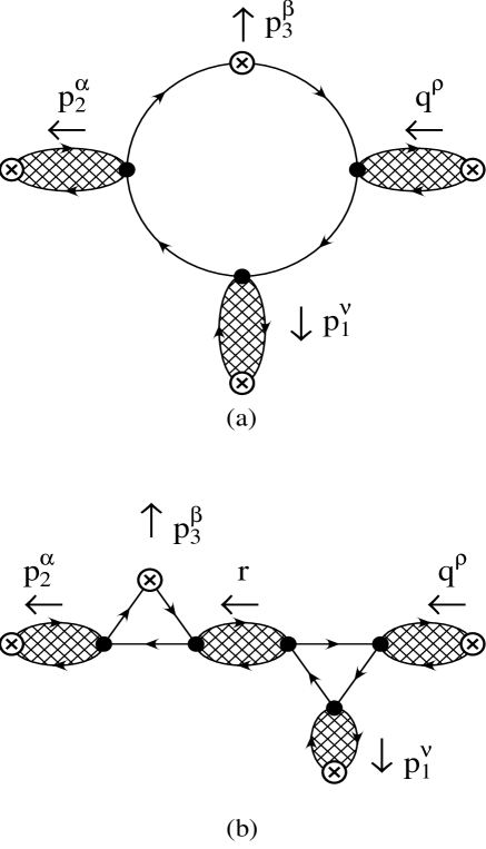
Figure 3: The two classes of hadronic light-by-light contributions to $a_{\mu}$ at leading ${\cal O}(N_{c})$. (a) The four-point functions class. (b) The product of two three-point functions class. The dots are ENJL vertices. The circled crossed vertices are where photons connect. The cross-hatched loops are full two-point functions and the lines are constituent quark propagators.

The second one, which we call three-point-like function contributions, can be regarded as two three-point functions glued with one full propagator (see Fig. 3(b)). Within this framework, it clearly appears that these two classes of contributions to the generalized four-point function $\Pi^{\rho\nu\alpha\beta}(p_{1},p_{2},p_{3})$ are different and therefore should be summed up [14]. The pure four-point function corresponds to the so-called quark loop contribution and the three-point-like function contributions to the meson pole exchange in the language of Ref. [20]. We remind that in our framework both classes of contributions to $\Pi^{\rho\nu\alpha\beta}(p_{1},p_{2},p_{3})$ are calculated to all orders in the CHPT expansion.

4.1 Pure Four-Point Function Contribution

This contribution is diagrammatically represented in Fig. 3(a). In the CHPT expansion the lowest order contribution is order $p^{8}$, thus potentially sensitive to the high energy region. The momenta assignment shown in the figure is the one corresponding to the first permutation. Whenever we give explicit expressions these are the ones corresponding to this permutation. The other five permutations are done analogously.

The pure four-point function is formed by a one-loop constituent quark vector four-point function ${\overline{\Pi}}^{\rho\nu\alpha\beta}(p_{1},p_{2},p_{3})$ with the same Lorentz and flavour structure as the four-point function in Eq. (2) with the three vector legs attaching to the muon line dressed with full vector propagators. These are the cross-hatched blobs in Fig. 3(b). The circled crosses vertices in the figure are where the photon lines connect. In the large $N_{c}$ limit there is either a constituent up, down or strange quark running in the loop. For a given quark flavour, this contribution to $\Pi^{\rho\nu\alpha\beta}(p_{1},p_{2},p_{3})$ can be written using the methods of [29] as,

$${}\Pi^{\rho\nu\alpha\beta}(p_{1},p_{2},p_{3})={\overline{\Pi}}_{abcd}(p_{1},p_{2},p_{3})\,{\cal V}^{abcd\rho\nu\alpha\beta}(p_{1},p_{2},p_{3})+\cdots$$ (4.1)

with

$${}{\cal V}^{abcd\rho\nu\alpha\beta}(p_{1},p_{2},p_{3}) \equiv \left(\frac{g^{a\rho}M_{V}^{2}(-q^{2})-q^{a}q^{\rho}}{M_{V}^{2}(-q^{2})-q^{2}}\right)\,\left(\frac{g^{b\nu}M_{V}^{2}(-p_{1}^{2})-p_{1}^{b}p_{1}^{\nu}}{M_{V}^{2}(-p_{1}^{2})-p_{1}^{2}}\right)$$

$$\times \left(\frac{g^{c\alpha}M_{V}^{2}(-p_{2}^{2})-p_{2}^{c}p_{2}^{\alpha}}{M_{V}^{2}(-p_{2}^{2})-p_{2}^{2}}\right)\,\left(\frac{g^{d\beta}M_{V}^{2}(-p_{3}^{2})-p_{3}^{d}p_{3}^{\beta}}{M_{V}^{2}(-p_{3}^{2})-p_{3}^{2}}\right)\,.$$

Dots stand for other possible contributions to $\Pi^{\rho\nu\alpha\beta}(p_{1},p_{2},p_{3})$. The indices $a,b,c,d,e,f$ stand in the remainder for Lorentz indices. The function $M_{V}^{2}(-p^{2})$ corresponds to either $\bar{u}u$, $\bar{d}d$ or $\bar{s}s$ flavour structure and can be found in Ref. [29]. Notice that the full vector propagators in the ENJL model have the same form as in VMD models but with a momentum dependent “vector mass”. See discussion in [29] about meson dominance in ENJL models.

After summing over all the six possible permutations of the external momenta only the terms proportional to $g_{\mu\nu}$ tensor survive because of the U(1) gauge invariance. This leads then to the phenomenological VMD rule of replacing the propagator of a photon with momentum $p$ by

$${}-\frac{g_{\mu\nu}}{p^{2}}\,\frac{M_{V}^{2}}{M_{V}^{2}-p^{2}}.$$ (4.3)

Thus implying that this rule preserves the Ward identities after summing over all the permutations.

We compute the one-constituent quark loop following the analysis in Appendix A and using a proper time regulator with a physical cut-off $\Lambda$.

The contribution of ${\overline{\Pi}}^{abcd}(p_{1},p_{2},p_{3})$ in eq. (4.1) to $a_{\mu}$ can be decomposed in terms of 32 independent amplitudes (see App. A). After integrating over the momentum running in the loop, these amplitudes will be integrals over the three Feynman parameters introduced by the standard procedure of reducing the four internal propagators to a power of one propagator. Moreover, after taking the derivative with respect to $p_{3\lambda}$ at $p_{3}=0$ one of the Feynman parameters can be integrated out analytically. The general form of each one of the 32 functions in ${\overline{\Pi}}^{abcd}(p_{1},p_{2},p_{3})$ for a constituent quark of flavour $i$ contributing to $a_{\mu}^{\rm light-by-light}$ is thus

$${}\frac{N_{c}}{16\pi^{2}}\,Q_{i}^{4}\,{\displaystyle\int^{1}_{0}}{\rm d}x{\displaystyle\int^{1-x}_{0}}{\rm d}y\,\frac{f(x,y)}{M^{4}(x,y)}\Gamma_{2}(M^{2}(x,y)/\Lambda^{2}),$$ (4.4)

where

$$M^{2}(x,y)\equiv M_{i}^{2}-x(1-x)(p_{1}+p_{2})^{2}-y(1-y)p_{2}^{2}+2xy(p_{1}+p_{2})\cdot p_{2},$$ (4.5)

and

$$\Gamma_{2}(\epsilon)=(1+\epsilon)e^{-\epsilon}\,.$$ (4.6)

Here $M_{i}$ is the constituent quark mass with flavour $i$. The Feynman parameters $x$ and $y$, together with the other five degrees of freedom for the two external muon loops in Eq. (2.6), produce a seven dimensional integral that we perform using the Monte Carlo routine VEGAS. The numerical results of this contribution will be discussed in Section 6.

As a check we have reproduced the results for the constituent quark and muon loops in [17] and the electron loop result in [41]. This is the calculation using (4.1) with ${\cal V}^{abcd\rho\nu\alpha\beta}=g^{a\rho}g^{b\nu}g^{c\alpha}g^{d\beta}$. We have also re-scaled the relevant masses. For the constituent quark mass we have used $M_{Q}=$ 300 MeV. The results are in Table 1. The numbers in brackets are the VEGAS quoted errors. The last row gives the known results.

Cut-off	$a_{\mu}\times 10^{7}$	$a_{\mu}\times 10^{9}$	$a_{\mu}\times 10^{9}$
$\mu$	Electron	Muon	Constituent Quark
(GeV)	Loop	Loop	Loop
0.5	2.41(8)	2.41(3)	0.395(4)
0.7	2.60(10)	3.09(7)	0.705(9)
1.0	2.59(7)	3.76(9)	1.10(2)
2.0	2.60(6)	4.54(9)	1.81(5)
4.0	2.75(9)	4.60(11)	2.27(7)
8.0	2.57(6)	4.84(13)	2.58(7)
Known Results	2.6252(4)	4.65	2.37(16)

Table 1: The results from a pure fermion loop compared with known numerical and analytical results. The known result for the electron loop has been partially analytically evaluated in [41], while the quoted values for the muon loop and the constituent quark loop are respectively analytical and numerical results of [17].

Within the numerical uncertainty of our calculation the agreement is good. It should be remarked that there are cancellations present at high energy. These contributions make the estimate numerically more uncertain for higher values of the cut-off $\mu$. As can be seen the electron loop has essentially reached its final value at a cut-off of 500 MeV. The same is not true for the muon loop or the constituent quark loop. The muon loop reaches its asymptotic value essentially at a cut-off of about 2 GeV. The constituent quark loop reaches its asymptotic value above 4 GeV. We have also calculated the same quantities for a few higher cut-offs and observed their stabilization within the numerical error. These sample calculations show that a proper study of the cut-off behaviour for the more difficult to estimate complete hadronic contribution is definitely necessary.

4.2 Three-Point-Like Function Contributions

This class of contributions is diagrammatically represented in Fig. 3(b). There are two permutations of the vector legs for each of the two three-point functions. In addition there are three possible sets of two momenta out of the four external vector legs momenta. This makes twelve possible permutations to be considered for three-point-like function contributions. The momenta shown in the figure are the ones corresponding to the first permutation. Whenever we give explicit expressions these are the ones corresponding to this permutation. The other eleven permutations are done analogously.

In this case we have two one-loop three-point functions with two vector legs each one glued with a full two-point function that can be either pseudoscalar, scalar, mixed pseudoscalar–axial-vector, or axial-vector. For intermediate vector two-point functions the result is zero because of Furry’s theorem. Three of the vector legs here are then attached to the muon line with dressed full vector propagators just as in the case of the pure four-point function discussed in the previous section. Again, in the large $N_{c}$ limit, there is either an up, down or strange constituent quark running in the loop. Technically we have used two different approaches to calculate this type of contributions. One is using the Ward identities for the four-point function $\Pi^{\rho\nu\alpha\beta}(p_{1},p_{2},p_{3})$. In this way one has to determine the 32 amplitudes of $\Pi^{\rho\nu\alpha\beta}(p_{1},p_{2},p_{3})$ contributing to $a_{\mu}^{\rm light-by-light}$, see Appendix A. The other way is constructing explicitly the complete $\Pi^{\rho\nu\alpha\beta}(p_{1},p_{2},p_{3})$ starting from the three- and two-point functions. Here one relies on the Ward identities for three-point functions. As a check we verified that both ways agree exactly.

In what follows we study each type of exchange (scalar, pseudoscalar and axial-vector) separately.

As an additional numerical check we have also calculated the pion exchange contribution with vector meson dominance of the rho meson in the vector legs and when the anomalous vertices are from the order $p^{4}$ Wess-Zumino effective action. Our result agrees exactly with that in Eq. (4.1) of [22] which quotes $-55.60(3)\cdot 10^{-11}$.

The two-point function involves the integration over one Feynman parameter and each one of the two three-point functions the integration over two more Feynman parameters. These integrals have been evaluated using Gaussian integration. To obtain $a_{\mu}$, one has to convolute these three-point-like contributions with the five dimensional space integral of the external two muon-loops in Eq. (2.6) which has been performed using the Monte Carlo routine VEGAS. The numerical results for these contributions will be discussed in Section 6.

4.2.1 Scalar Exchange

For the scalar exchange, the lowest order contribution in the CHPT expansion is order $p^{8}$. This contribution to $\Pi^{\rho\nu\alpha\beta}(p_{1},p_{2},p_{3})$ can be written as

$${}\Pi^{\rho\nu\alpha\beta}(p_{1},p_{2},p_{3}) = \!{\overline{\Pi}}_{ab}^{VVS}(p_{1},r)g_{S}\left(1+g_{S}\Pi^{S}(r)\right){\overline{\Pi}}_{cd}^{SVV}(p_{2},p_{3}){\cal V}^{abcd\rho\nu\alpha\beta}(p_{1},p_{2},p_{3})$$

$$+\cdots,$$

where ${\cal V}^{abcd\rho\nu\alpha\beta}(p_{1},p_{2},p_{3})$ has been defined in Eq. (4.1) and $r=p_{2}+p_{3}$. The full two-point function $\Pi^{S}(p)$ can be found in Ref. [30] and the one-loop three-point functions ${\overline{\Pi}}^{VVS}_{\mu\nu}(p,q)$ and ${\overline{\Pi}}^{SVV}_{\mu\nu}(p,q)$ are in Appendix B. Eq. (4.2.1) can be understood as follows: $g_{S}(1+g_{S}\Pi^{S}(r))$ is the scalar propagator connecting the two vertices ${\overline{\Pi}}_{cd}^{SVV}(p_{2},p_{3})$ and ${\overline{\Pi}}_{ab}^{VVS}(p_{1},r)$. The whole diagram is then glued to the external photon lines with the vector propagators given by ${\cal V}^{abcd\rho\nu\alpha\beta}$.

4.2.2 Pseudoscalar Exchange

For the pseudoscalar exchange the lowest order contribution in the CHPT expansion is order $p^{6}$. This, together with the fact that it involves two flavour anomalous vertices points out that this contribution could be the leading one. Considering as part of the pseudoscalar exchange all those terms proportional to a pseudoscalar propagator, this contribution also includes the pseudoscalar–axial-vector mixed terms. Its expression is given by

$${}\Pi^{\rho\nu\alpha\beta}(p_{1},p_{2},p_{3}) = \left[{\overline{\Pi}}_{ab}^{VVP}(p_{1},r)\left(1+g_{S}\Pi^{P}(r)\right){\overline{\Pi}}_{cd}^{PVV}(p_{2},p_{3})\right.$$ (4.8)

$$-g_{V}{\overline{\Pi}}_{ab}^{VVP}(p_{1},r)\Pi^{P\mu}(r){\overline{\Pi}}_{\mu cd}^{AVV}(p_{2},p_{3})$$

$$-g_{V}\left.{\overline{\Pi}}_{ab\mu}^{VVA}(p_{1},r)\Pi^{P\mu}(-r){\overline{\Pi}}_{cd}^{PVV}(p_{2},p_{3})\right]$$

$$\times g_{S}{\cal V}^{abcd\rho\nu\alpha\beta}(p_{1},p_{2},p_{3})+\cdots$$

where ${\cal V}^{abcd\rho\nu\alpha\beta}(p_{1},p_{2},p_{3})$ has been defined in Eq. (4.1) and $r=p_{2}+p_{3}$. The full two-point functions $\Pi^{P}(p)$ and $\Pi^{P}_{\mu}(p)$ and the one-loop three-point functions ${\overline{\Pi}}^{PVV}_{\mu\nu}(p,q)$ and ${\overline{\Pi}}^{VVP}_{\mu\nu}(p,q)$ can be found in Ref. [29]. See Eq. (B.5) in Appendix B for the explicit expression. The mixed two-point function $\Pi^{P}_{\mu}(p)$ can be written as [29],

$$\Pi^{P}_{\mu}(p)\equiv ip_{\mu}\,\Pi^{P}_{M}(p^{2}).$$ (4.9)

Since both the $VVA$ and the $AVV$ one-loop three-point functions are multiplied by $r_{\mu}$, we use the one-loop anomalous Ward identity in Eq. (4.24) of [29] and the prescription given in [30] to rewrite Eq. (4.8) as

$${}\Pi^{\rho\nu\alpha\beta}(p_{1},p_{2},p_{3}) = g_{S}{\overline{\Pi}}_{ab}^{VVP}(p_{1},r)\left(1+g_{S}\Pi^{P}(r)-4g_{V}M_{i}\Pi^{P}_{M}(r^{2})\right)$$ (4.10)

$$\times{\overline{\Pi}}_{cd}^{PVV}(p_{2},p_{3})\,{\cal V}^{abcd\rho\nu\alpha\beta}(p_{1},p_{2},p_{3})$$

$$+ 2M_{Q}g_{S}g_{V}\Pi^{P}_{M}(r^{2})\left[{\overline{\Pi}}_{ab}^{VVP}(p_{1},r)\left\{{\overline{\Pi}}_{cd}^{PVV}(p_{2},p_{3}){\left.\right|^{M_{i}=M_{Q}}_{p_{2}^{2}=p_{3}^{2}=r^{2}=0}}\right\}\right.$$

$$\times \left(\frac{g^{a\rho}M_{V}^{2}(-q^{2})-q^{a}q^{\rho}}{M_{V}^{2}(-q^{2})-q^{2}}\right)\,\left(\frac{g^{b\nu}M_{V}^{2}(-p_{1}^{2})-p_{1}^{c}p_{1}^{\nu}}{M_{V}^{2}(-p_{1}^{2})-p_{1}^{2}}\right)g^{c\alpha}g^{d\beta}\,$$

$$+ \left\{{\overline{\Pi}}^{ab}_{VVP}(p_{1},r){\left.\right|^{M_{i}=M_{Q}}_{p_{1}^{2}=r^{2}=q^{2}=0}}\right\}{\overline{\Pi}}^{cd}_{PVV}(p_{2},p_{3})$$

$$\times \left.g^{a\rho}g^{b\nu}\left(\frac{g^{c\alpha}M_{V}^{2}(-p_{2}^{2})-p_{2}^{c}p_{2}^{\alpha}}{M_{V}^{2}(-p_{2}^{2})-p_{2}^{2}}\right)\left(\frac{g^{d\beta}M_{V}^{2}(-p_{3}^{2})-p_{3}^{d}p_{3}^{\beta}}{M_{V}^{2}(-p_{3}^{2})-p_{3}^{2}}\right)\right]$$

$$+ \cdots\,,$$

where $M_{i}$ is the constituent quark mass for the quark with flavour $i$ and $M_{Q}$ its value in the chiral limit. The first two lines above come from applying naive Ward identities to the axial-vector leg, while the remaining contributions are the subtractions needed to fulfil the anomalous Ward identities. In addition, ${\overline{\Pi}}^{PVV}_{\mu\nu}(p,q)$ contains subtractions also determined by the anomalous Ward identities [29]. See Eq. (B) in Appendix B. The expression (4.10) also shows that the pseudoscalar exchange contribution always contains at least one vector meson propagator. Due to this fact and the presence of the subtractions in (4.10), the $\pi^{0}\gamma^{*}\gamma^{*}$ vertex goes to a constant when the vector legs’ Euclidean momenta are very large. Therefore, although this contribution when summed over all possible permutations is convergent by itself because of gauge invariance (see Section 2), the subtraction terms make it very slowly convergent. We know that in QCD the $\pi^{0}\gamma^{*}\gamma^{*}$ vertex goes like $1/Q^{2}$ at large Euclidean momentum [42]. This behaviour is also supported by the measured $\pi^{0}\gamma\gamma^{*}$ form factor in the Euclidean region at CELLO [43] and CLEO-II [44] detectors. This indicates again that although this model gives the right contribution for energies below or around $\Lambda$, it breaks down above. We shall estimate the intermediate and high energy region contributions for the pseudoscalar exchange in Section 6.

Although the present section is devoted to the large $N_{c}$ contributions, it is worth to discuss the main $1/N_{c}$ corrections to the pseudoscalar exchange at this point. These are the effects of the U(1)_A anomaly and were already included in the Erratum in Ref. [21]. In the chiral limit and in the large $N_{c}$ limit there are nine pseudo-Goldstone bosons [32]: $\pi^{\pm}$, $\pi^{0}$, $K^{\pm}$, $K^{0}$, $\overline{K}^{0}$, $\eta_{8}$ and $\eta_{1}$. Under flavour SU(3) they transform as a nonet multiplet. However nonet symmetry is broken by $1/N_{c}$ effects due to the U(1)_A anomaly. These effects cause the isospin zero mass eigenstates to become the $\eta$ and $\eta^{\prime}$ states. They also increase the mass of the $\eta^{\prime}$ meson to 958 MeV. These $1/N_{c}$ corrections are thus quite relevant to the pseudoscalar exchange. We have taken them into account by using the physical $\pi^{0}$, $\eta$ and $\eta^{\prime}$ mass eigenstates as propagating states. This already gives the bulk of the effects of the U(1)_A anomaly. Higher order corrections are negligible and within the quoted error. The results of using either $\bar{u}u$, $\bar{d}d$, and $\bar{s}s$ basis of states for the large $N_{c}$ limit or the physical $\pi^{0}$, $\eta$ and $\eta^{\prime}$ basis are given in Section 6.

4.2.3 Axial-Vector Exchange

For the axial-vector exchange, the lowest order contribution in the CHPT expansion is order $p^{8}$. This contribution to $\Pi^{\rho\nu\alpha\beta}(p_{1},p_{2},p_{3})$ can be written as

$${}\Pi^{\rho\nu\alpha\beta}(p_{1},p_{2},p_{3}) = -g_{V}\,{\overline{\Pi}}_{abe}^{VVA}(p_{1},r)\left(g^{ef}-g_{V}\Pi_{A}^{ef}(r)\right){\overline{\Pi}}_{fcd}^{AVV}(p_{2},p_{3})$$ (4.11)

$$\times{\cal V}^{abcd\rho\nu\alpha\beta}(p_{1},p_{2},p_{3})+\cdots$$

where ${\cal V}^{abcd\rho\nu\alpha\beta}(p_{1},p_{2},p_{3})$ has been defined in Eq. (4.1) and $r=p_{2}+p_{3}$. The full axial-vector two-point function $\Pi_{A}^{\mu\nu}(p)$ can be found in Ref. [29] and the one-loop three-point functions ${\overline{\Pi}}^{VVA}_{\mu\nu\alpha}(p,q)$ and ${\overline{\Pi}}^{AVV}_{\mu\nu\alpha}(p,q)$ are in Appendix B.

Using the one-loop anomalous Ward identity in Eq. (4.24) of [29] and the prescription given in [30] for the terms in (4.11) where $r_{\mu}$ multiplies either the $VVA$ or the $AVV$ three-point functions, we can rewrite (4.11) as

$${}\Pi^{\rho\nu\alpha\beta}(p_{1},p_{2},p_{3}) = -g_{V}\,{\overline{\Pi}}_{abe}^{VVA}(p_{1},r)g^{ef}\left(1+g_{V}r^{2}\Pi_{A}^{(1)}(-r^{2})\right){\overline{\Pi}}_{fcd}^{AVV}(p_{2},p_{3})$$ (4.12)

$$\times{\cal V}^{abcd\rho\nu\alpha\beta}(p_{1},p_{2},p_{3})-2g_{V}^{2}\left(\Pi_{A}^{(0)}(-r^{2})+\Pi_{A}^{(1)}(-r^{2})\right)$$

$$\times \left\{\left(\frac{g^{a\rho}M_{V}^{2}(-q^{2})-q^{a}q^{\rho}}{M_{V}^{2}(-q^{2})-q^{2}}\right)\,\left(\frac{g^{b\nu}M_{V}^{2}(-p_{1}^{2})-p_{1}^{c}p_{1}^{\nu}}{M_{V}^{2}(-p_{1}^{2})-p_{1}^{2}}\right)\right.$$

$$\left.M_{i}{\overline{\Pi}}_{ab}^{VVP}(p_{1},r)-M_{Q}{\overline{\Pi}}^{\rho\nu}_{VVP}(p_{1},r){\left.\right|^{M_{i}=M_{Q}}_{p_{1}^{2}=r^{2}=q^{2}=0}}\,\right\}$$

$$\times \left\{\left(\frac{g^{c\alpha}M_{V}^{2}(-p_{2}^{2})-p_{2}^{c}p_{2}^{\alpha}}{M_{V}^{2}(-p_{2}^{2})-p_{2}^{2}}\right)\,\left(\frac{g^{d\beta}M_{V}^{2}(-p_{3}^{2})-p_{3}^{d}p_{3}^{\beta}}{M_{V}^{2}(-p_{3}^{2})-p_{3}^{2}}\right)\right.$$

$$\left.M_{i}{\overline{\Pi}}_{cd}^{PVV}(p_{2},p_{3})-M_{Q}{\overline{\Pi}}^{\alpha\beta}_{PVV}(p_{2},p_{3}){\left.\right|^{M_{i}=M_{Q}}_{p_{2}^{2}=p_{3}^{2}=r^{2}=0}}\right\}$$

$$+ \cdots\,.$$

The expression for the two-point axial amplitudes $\Pi_{A}^{(0)}(-r^{2})$ and $\Pi_{A}^{(1)}(-r^{2})$ can be found in [29]. The kinematical pole of the transverse part at $r^{2}=0$ disappears in the combinations $1+g_{V}r^{2}\Pi_{A}^{(1)}(-r^{2})$ and $\Pi_{A}^{(0)}(-r^{2})+\Pi_{A}^{(1)}(-r^{2})$. The last combination contains a pseudoscalar propagator which is often included in the pseudoscalar exchange contribution.

5 Low Energy Next-to-Leading in $1/N_{c}$ Contributions

In this section we discuss the low energy next-to-leading in $1/N_{c}$ contributions to $a_{\mu}^{\rm light-by-light}$. In the previous sections we have discussed the low energy large $N_{c}$ contributions in the context of the ENJL model. We included the effects of the U(1)_A anomaly which are next-to-leading in $1/N_{c}$ as well. Here we address the calculation of the other ${\cal O}(1)$ corrections in the $1/N_{c}$ expansion. In the language of the ENJL model, these corrections are given by loops of strings of quark bubbles. They contain one closed loop of a string of bubbles like the one in Fig. 2(a). This loop is then connected in all possible ways to the photons using strings of bubbles. In a mesonic picture they correspond to one meson loop contributions. This meson loop can then substitute any one-loop constituent quark (bubble) in diagrams in Figs. 3(a) and 3(b). We end up with two classes of $O(1)$ contributions. The $1/N_{c}$ next-to-leading corrections to the full two-point functions, i.e. to meson masses and couplings and the $1/N_{c}$ next-to-leading corrections to the three- and four-point one-loop functions, i.e. to vertices. In fact, the major $1/N_{c}$ correction to pseudoscalar two-point functions, namely the U(1)_A anomaly, was already estimated in Section 4. The other $1/N_{c}$ corrections to two-point functions should be small since the phenomenological analysis in Refs. [28, 33] and [29] fits very well. We thus expect these to be already included in the error of the model for the large $N_{c}$ results. Therefore, we shall only consider here the $1/N_{c}$ corrections to the vertices.

Unfortunately, at present, these type of contributions cannot be fully treated in the ENJL model. Some of the reasons were given in Section 3. In its present form the ENJL model we are using is just well defined in the large $N_{c}$ limit. However, the fact that these type of contributions are of different large $N_{c}$ counting with respect to the ones treated in Section 4, permits the separate treatment we follow below for them.

Four-point functions can be also calculated at very low energy within CHPT [46]. In this regime the relevant degrees of freedom are the lowest pseudoscalar mesons, while vector, axial-vector and scalar resonances have been integrated out. Their effects are included in the couplings of the CHPT Lagrangian [47]. CHPT becomes then a good tool to study strong interactions of the lowest pseudoscalar mesons with external sources. In this framework we need both $\gamma^{*}P^{+}P^{-}$ and $\gamma^{*}\gamma^{*}P^{+}P^{-}$ vertices, where $P$ is pion or kaon. The first vertex is well known phenomenologically and VMD models give a very good description of it. On the contrary, not much is known phenomenologically about the second one. This fact induces a large model dependence since one can construct many models satisfying the relevant Ward identities and with different degrees of VMD. One can use for instance the HGS model as in [20] where there is no complete VMD for the $\gamma^{*}\gamma^{*}P^{+}P^{-}$ vertex. We shall discuss this contribution in a complete VMD model both for $\gamma^{*}P^{+}P^{-}$ and $\gamma^{*}\gamma^{*}P^{+}P^{-}$ vertices. This is done inspired by the form of the ${\cal O}(N_{c})$ contributions in the ENJL model.

In previous sections we have seen that the most general expression for the four-point function $\Pi^{\rho\nu\alpha\beta}(p_{1},p_{2},p_{3})$ at ${\cal O}(N_{c})$ in the ENJL model contains the one-loop four- or three-point-like functions, which give the lowest order in the CHPT counting, multiplied by the ENJL vector meson propagators in Eq. (4.1). Inspired by this behaviour we saturate the ${\cal O}(1)$ contribution by one loop of charged pion or kaon mesons using lowest order CHPT photon-pion vertices, i.e. ${\cal O}(p^{2})$, multiplied by the ENJL vector meson propagators in (4.1). The main difference with a full ENJL calculation here is that we substitute the momentum dependent pion mass and coupling by their experimental values.

To understand the sensitivity to the momenta dependence of the vector meson propagators we have numerically studied the difference between the case with vector propagators containing a constant vector mass and the case with a momentum dependent one. Each choice gives different high energy behaviour of the photon-pion vertices.

For the pseudo-Goldstone bosons loops contribution to $\Pi^{\rho\nu\alpha\beta}(p_{1},p_{2},p_{3})$, the lowest order in the CHPT counting is order $p^{4}$. This also points out that this contribution could be dominated by lower energy regions than the other contributions analyzed in previous sections which started at order $p^{6}$. Since we are including as propagating states only the lowest pseudoscalar mesons and the rho vector, our approach will be only valid for energies below or around 1 GeV. Above this energy axial-vector mesons become also dynamical states. The saturation of this contribution from physics at scales around 1 GeV can only be confirmed a posteriori. The numerical results concerning this contribution are presented in Section 6.

We now proceed to analyze in more detail the two types of possible contributions: the pure four-point function and three-point-like function contributions. In particular, the three-point-like contributions can be seen as the diagram in Figure 3(b) where one or both one-constituent-quark loop three-point functions are replaced with charged pion or kaon loops. Due to parity, the intermediate two-point function glueing the two three-point functions can be either vector or scalar. The vector contribution is again zero because of Furry’s theorem (this can be better verified in the ENJL inspired diagrams where the vector legs couple to fermion lines). The scalar contribution we expect to be very much suppressed like in the ${\cal O}(N_{c})$ case (see numerical results in Section 6). The important point here is that there are no anomalous contributions since now we have mesons running in the three-point functions. This makes this contribution to be in the range of the expected CHPT counting and not anomalously large as we obtained for the ${\cal O}(N_{c})$ pseudoscalar exchange.

Therefore we only estimate the dominant pure four-point function contribution to $\Pi^{\rho\nu\alpha\beta}(p_{1},p_{2},p_{3})$ in Eq. (2). This can be seen as the diagram in Fig. 3(a) where the one-loop constituent quark four-point function is now a loop of pseudoscalar mesons. It can be written as

$${}\Pi^{\rho\nu\alpha\beta}(p_{1},p_{2},p_{3})={\overline{\Pi}}_{abcd}(p_{1},p_{2},p_{3})\,{\cal V}^{abcd\rho\nu\alpha\beta}(p_{1},p_{2},p_{3})+\cdots$$ (5.1)

where ${\overline{\Pi}}_{abcd}(p_{1},p_{2},p_{3})$ is the ${\cal O}(1)$ in $1/N_{c}$ contribution from charged pion and kaon loops using lowest order in CHPT photon-pion vertices. For that, we compute at lowest order in CHPT, the quark vector current appearing in the definition of $\Pi^{\rho\nu\alpha\beta}(p_{1},p_{2},p_{3})$ [46]

$$V^{\mu}_{a}(x)\Rightarrow iQ_{a}\left(\left[\pi^{+}(x),D^{\mu}\pi^{-}(x)\right]+\left[K^{+}(x),D^{\mu}K^{-}(x)\right]\right)_{aa}\,,$$ (5.2)

where the subscript $aa$ means that we take the $aa$ component in flavour space. Due to the covariant derivative $D_{\mu}P\equiv\partial_{\mu}P-i|e|[A_{\mu},P]$, the term above gives rise both to $P^{+}P^{-}\gamma^{*}$ and $P^{+}P^{-}\gamma^{*}\gamma^{*}$ vertices. Of course, the full contribution to $\Pi^{\rho\nu\alpha\beta}(p_{1},p_{2},p_{3})$ at a given order in CHPT, in this case ${\cal O}(p^{2})$, has to be gauge covariant. We construct the one-loop four-point function ${\overline{\Pi}}_{abcd}(p_{1},p_{2},p_{3})$ following again the analysis in Appendix A, where we need to determine the 32 independent amplitudes that contribute to the $a^{\rm light-by-light}_{\mu}$. These amplitudes have always the Lorentz indices saturated by external momenta indices. Notice that vertices with one photon are proportional to external momenta, while vertices with two photons are proportional to $g_{\mu\nu}$ tensors. Thus we only need to compute the UV convergent amplitudes and reconstruct the contribution from the two-photons–two-mesons vertices by using gauge invariance. The full meson one-loop with order $p^{2}$ vertices explicitly satisfies the chiral and U(1) gauge Ward identities. In fact the amplitudes one gets for the 32 independent functions are very similar to the ones found in the one-loop constituent quark amplitudes in Eq. (4.4). The general form we obtain for them is

$${}-\frac{1}{16\pi^{2}}\left(Q_{u}-Q_{d}\right)^{4}{\displaystyle\int^{1}_{0}}{\rm d}x{\displaystyle\int^{1-x}_{0}}{\rm d}y\,\frac{g(x,y)}{\tilde{M}^{4}(x,y)},$$ (5.3)

with

$$\tilde{M}^{2}(x,y)\equiv m_{P}^{2}-x(1-x)(p_{1}+p_{2})^{2}-y(1-y)p_{2}^{2}+2xy(p_{1}+p_{2})\cdot p_{2}$$ (5.4)

and $m_{P}$ is the mass of the pseudoscalar meson $P$. The one-loop meson pure four-point function is multiplied with the propagator in (4.1) to give the full four-point function of Eq. (5.1).

If the one-loop four-point function satisfies the Ward identities, as it does, also the full four-point function (5.1) will satisfy them since

$$q_{\mu}\,\left(g^{\mu\nu}M_{V}^{2}-q^{\mu}q^{\nu}\right)=q^{\nu}\left(M_{V}^{2}-q^{2}\right)\,,$$ (5.5)

independently of whether $M_{V}$ is momentum dependent or not. As we already said for the one-loop constituent quark loop contribution, after summing over all possible permutations of the three vector legs, only the terms proportional to $g_{\mu\nu}$ in (4.1) survive since the meson one-loop four-point function satisfies the Ward identities. This leaves the phenomenologically VMD rule in Eq. (4.3) to work here too. This eliminates the worries about the fulfilling of chiral symmetry when using this substitution [19, 20].

That this procedure is fully chiral and U(1) gauge invariant can be seen simply by constructing a Lagrangian with full electromagnetic gauge and chiral invariance and that has complete VMD for both $\gamma P^{+}P^{-}$ and $\gamma\gamma P^{+}P^{-}$ vertices. The following Lagrangian contains couplings of pions and photons to all orders in external momenta and reproduces the full VMD amplitude without inducing any extra vertices of photons and pseudoscalar mesons.

$${}{\cal L}_{\mbox{VMD}} = \frac{f_{\pi}^{2}}{4}\mathrm{tr}\left({\cal D}_{\mu}U{\cal D}^{\mu}U^{\dagger}+\chi U^{\dagger}+U\chi^{\dagger}\right)$$ (5.6)

$$+ \sum_{n\geq 0}ia_{n}\mathrm{tr}\left[\left({\cal D}^{2n}{\cal D}^{\mu}L_{\mu\nu}\right)U^{\dagger}{\cal D}^{\nu}U+\left({\cal D}^{2n}{\cal D}^{\mu}R_{\mu\nu}\right)U{\cal D}^{\nu}U^{\dagger}\right]$$

$$+ \sum_{n,m\geq 0}b_{nm}\mathrm{tr}\left[\left({\cal D}^{2n}{\cal D}_{\mu}L^{\mu\nu}\right)U^{\dagger}\left({\cal D}^{2m}{\cal D}^{\alpha}R_{\alpha\nu}\right)U\right].$$

The $3\times 3$ flavour matrix $U$ contains the pseudoscalar meson fields [46] and

$${\cal D}_{\mu}U=\partial_{\mu}U-i(v_{\mu}+a_{\mu})U+iU(v_{\mu}-a_{\mu})\,.$$ (5.7)

Here $v_{\mu}$, $a_{\mu}$ are external vector and axial-vector fields, while the field $\chi=2~{}B_{0}{\cal M}+...$ contains the current quark mass matrix ${\cal M}$. The photon field is contained in $v_{\mu}$.

The field strengths $R(L)_{\mu\nu}$ are constructed out of the fields $r(l)_{\mu}=v_{\mu}+(-)a_{\mu}$. The covariant derivatives act on $R(L)_{\mu\nu}$ as follows

$${\cal D}_{\alpha}R(L)_{\mu\nu}=\partial_{\alpha}R(L)_{\mu\nu}-i[r(l)_{\alpha},R(L)_{\mu\nu}].$$ (5.8)

The form of the terms in (5.6) has been chosen such that there are no vertices with three or more photons interacting with pions generated. The first line is the lowest order CHPT Lagrangian. The second line contains one- or two-photons couplings to pseudoscalar mesons while the last line contains only two-photons couplings to pseudoscalar mesons.

The vertex for a charged pion with incoming momentum $p$ and a photon with outgoing momentum $k$ and polarization $\epsilon^{\mu}$ is given by

$$i|e|\left(2p-k\right)^{\nu}\left\{g_{\mu\nu}+\left(k^{2}g_{\mu\nu}-k_{\mu}k_{\nu}\right)\frac{2}{f_{\pi}^{2}}\sum_{n\geq 0}a_{n}\left(-k^{2}\right)^{n}\right\}\,.$$ (5.9)

The first term is the lowest order vertex. With the choice

$$a_{n}=-\frac{f_{\pi}^{2}}{2}\left(\frac{-1}{M_{V}^{2}}\right)^{n+1}$$ (5.10)

this reproduces the phenomenological complete VMD behaviour for the $\gamma^{*}P^{+}P^{-}$ vertex. But notice that any VMD-like $M_{V}^{2}(k^{2})/(M_{V}^{2}(k^{2})-k^{2})$ behaviour, with $M_{V}^{2}(0)\neq 0$, as the one obtained in the ENJL model can be reproduced by choosing the $a_{n}$ appropriately. I.e.

$$\frac{2}{f_{\pi}^{2}}\sum_{n\geq 0}a_{n}\left(-k^{2}\right)^{n}=\frac{1}{M_{V}^{2}(k^{2})-k^{2}}.$$ (5.11)

We now turn to the $\gamma^{*}\gamma^{*}P^{+}P^{-}$ vertex. If the two photons outgoing momenta are $k_{1}$ and $k_{2}$ and their polarizations $\epsilon^{\mu}$ and $\epsilon^{\nu}$ respectively, that vertex is given by

$$2ie^{2}g_{\mu\nu}$$ (5.12)

$$+4i\frac{e^{2}}{f_{\pi}^{2}}\,\left(k_{1}^{2}g_{\mu\nu}-k_{1\mu}k_{1\mu}\right)\sum_{n\geq 0}a_{n}\left(-k_{1}^{2}\right)^{n}$$

$$+4i\frac{e^{2}}{f_{\pi}^{2}}\,\left(k_{2}^{2}g_{\mu\nu}-k_{2\mu}k_{2\nu}\right)\sum_{n\geq 0}a_{n}\left(-k_{2}^{2}\right)^{n}$$

$$-2i\frac{e^{2}}{f_{\pi}^{2}}\,\left(k_{1}^{2}g_{\mu}^{.\alpha}-k_{1\mu}k_{1}^{\alpha}\right)\left(k_{2}^{2}g_{\alpha\nu}-k_{2\alpha}k_{2\nu}\right)$$

$$\times \sum_{n,m\geq 0}b_{nm}\left[\left(-k_{1}^{2}\right)^{n}\left(-k_{2}^{2}\right)^{m}+\left(-k_{2}^{2}\right)^{n}\left(-k_{1}^{2}\right)^{m}\right]\,.$$

Here we see that, keeping gauge and chiral invariance fully satisfied, this vertex is rather unconstrained. The choice $b_{nm}=0$ reproduces the HGS model used in [20, 22] with $a=2$. The difference between that model and the complete VMD model only starts at order $p^{6}$ in the chiral counting.

A large number of other choices are however possible. In particular the choice

$$b_{nm}=-\frac{2}{f_{\pi}^{2}}\,a_{n}\,a_{m}$$ (5.13)

reproduces the complete VMD amplitude for $\gamma^{*}\gamma^{*}P^{+}P^{-}$ used in this work. Again depending on the coefficients $a_{n}$, one can have the ENJL vector meson propagator or any other one like the phenomenological complete VMD mentioned above. For comparison we use both, see Section 6. It is also possible to add chiral invariant terms that will produce a direct dependence on $k_{1}\cdot k_{2}$. This last possibility is realized by adding terms like

$$\left({\cal D}^{2n}{\cal D}^{\beta}{\cal D}^{\mu}L_{\mu\nu}\right)U^{\dagger}\left({\cal D}^{2m}{\cal D}_{\beta}{\cal D}^{\alpha}R_{\alpha\nu}\right)U.$$ (5.14)

The numerical results for the pseudoscalar mesons loops contribution are discussed in Section 6.

6 Numerical Results

In this section we give the numerical results for the low energy calculation of the hadronic light-by-light contributions to $a_{\mu}$ presented in Sections 4 and 5.

We first analyze the result for the large $N_{c}$ limit calculation including the effects of the U(1)_A anomaly as explained in Section 4. Since we are dealing with a low-energy model, as mentioned before, it is necessary to study the dependence on a high-energy cut-off $\mu$ on the vector legs’ momenta.

For the seven dimensional integral of the pure four-point function (or one constituent quark loop) contribution, we used a statistics of 20 iterations with $10^{5}$ points in the Monte Carlo routine VEGAS, while for the two muon loops five dimensional integral of the three-point-like function contributions we used a statistics of 20 iterations with 5000 points in the same Monte Carlo routine. This statistics is equivalent to the one used in the seven dimensional integral case. For the two- and three-point functions needed in these three-point-like contributions we used Gaussian integration with an accuracy of $10^{-6}$.

6.1 Pure Four-Point Function

In Table 2 we have listed the leading hadronic light-by-light ${\cal O}(N_{c})$ contributions to $a_{\mu}$, i.e the pure four-point function in the second column and the pseudoscalar exchange three-point-like function in the third column, as a function of the cut-off together with the errors quoted by VEGAS.

Cut-off	$a_{\mu}$ $\times$ $10^{10}$ from	$a_{\mu}$ $\times$ $10^{10}$ from	$a_{\mu}$ $\times$ $10^{10}$ from	$a_{\mu}$ $\times$ $10^{10}$
$\mu$	Constituent	Pseudoscalar	$\pi^{0}$, $\eta$ and $\eta^{\prime}$
(GeV)	Quark	Exchange ${\cal O}(N_{c})$	Exchanges	Sum
	in Figure 3(a)	in Figure 3(b)	${\cal O}(N_{c})$ + U(1)A
0.5	0.78(0.01)	$-$14.2(0.1)	$-$4.8(0.1)	$-$4.0
0.7	1.14(0.02)	$-$19.4(0.1)	$-$6.8(0.1)	$-$5.7
1.0	1.44(0.03)	$-$24.2(0.2)	$-$9.0(0.1)	$-$7.6
2.0	1.78(0.04)	$-$33.0(0.2)	$-$12.6(0.2)	$-$10.8
4.0	1.98(0.05)	$-$39.6(0.6)	$-$15.0(0.2)	$-$13.0
8.0	2.00(0.08)	$-$46.3(1.5)	$-$17.6(0.4)	$-$15.6

Table 2: Results for the order $N_{c}$ constituent quark loop and pseudoscalar exchange hadronic light-by-light contributions to $a_{\mu}$ in the ENJL model.

Since the integrand is rather irregular, this error estimate is somewhat on the small side (see also [48]) and will be largely superseded by the error in our final result.

For the bare constituent quark loop, the result only stabilizes at a rather high value of $\mu$. For instance, for a bare quark loop with a constituent quark mass of 300 MeV, the change between a cut-off of 2 GeV to a cut-off of 4 GeV is still typically 20%. The change from 0.7 GeV to 2 GeV is typically a factor of 1.8. These are the results quoted in column 4 of Table 1. The changes for our more realistic ENJL model four-point function can be judged from the results in Table 2, column 2. It still has a significant change between 1 and 2 GeV cut-off. This invalidates the use of any low energy model to calculate accurately the complete hadronic light-by-light contribution to $a_{\mu}$. The bulk of these contributions does not come from the dynamics at scales around the muon mass as it is often stated. This also explains the rather high sensitivity to the damping provided by the vector two-point functions as seen in [17]. Mostly due to its electric charge and heavier mass, the contribution of the strange quark flavour is much smaller (around $0.04\cdot 10^{-10}$) than that of the up and down quarks shown in the Table 2. This value is within the quoted VEGAS error for up and down quark contributions. In Section 7 we give an estimate of the intermediate and high energy one constituent light quark loop contributions and the heavier quark flavours contributions.

6.2 Pseudoscalar Three-Point-Like Function

For the three-point-like function contributions we have done the same study of the cut-off dependence as for the four-point function contribution. In particular we find that at large $N_{c}$ the contribution of the pseudoscalar exchange is more than one order of magnitude larger than the others. The reason this contribution is so different can be traced back both to the presence of two flavour anomaly vertices and the CHPT counting. It therefore deserves more attention. In fact, the pseudoscalar exchange has important next-to-leading corrections from the effects of the U(1)_A anomaly that leave the $\pi^{0}$ exchange as the dominant contribution to $a_{\mu}^{\rm light-by-light}$. First we give in column 3 of Table 2 the result strictly to leading order in $1/N_{c}$ from the $u,d$ and $s$ flavours.

We have taken into account the effects of the U(1)_A anomaly by using the physical $\pi^{0}$, $\eta$ and $\eta^{\prime}$ mass eigenstates as propagating states instead of the $\bar{u}u$, $\bar{d}d$ and $\bar{s}s$ in the large $N_{c}$ limit. This includes the main effect of the U(1)_A anomaly which is in the differences of the masses of the pseudoscalar $\eta$ and $\eta^{\prime}$ mesons. In the $\pi^{0}$, $\eta$ and $\eta^{\prime}$ basis, the contribution from the pion intermediate state has a charge factor $\left[\left((2/3)^{2}-(-1/3)^{2}\right)/\sqrt{2}\right]^{2}$ compared to a single quark of charge one. We thus multiply the ENJL pseudoscalar exchange result of column 3 in (2) by this factor to obtain the $\pi^{0}$ contribution from the ENJL model listed in column 2 of Table 3.

Cut-off	$a_{\mu}\times 10^{10}$	$a_{\mu}\times 10^{10}$	$a_{\mu}\times 10^{10}$	$a_{\mu}\times 10^{10}$
$\mu$
(GeV)	ENJL	Point-Like–VMD ($\pi^{0}$)	$\eta$	$\eta^{\prime}$
0.4	$-$2.84(2)	$-$2.70(1)	$-$0.425(1)	$-$0.266(1)
0.5	$-$3.70(3)	$-$3.46(2)	$-$0.616(2)	$-$0.399(2)
0.7	$-$5.04(4)	$-$4.49(3)	$-$0.923(3)	$-$0.631(2)
1.0	$-$6.44(7)	$-$5.18(3)	$-$1.180(4)	$-$0.847(3)
2.0	$-$8.83(17)	$-$5.62(5)	$-$1.37(1)	$-$1.03(1)
4.0	$-$10.51(37)	$-$5.58(5)	$-$1.38(1)	$-$1.04(1)

Table 3: The $\pi^{0}$ exchange contribution to $a_{\mu}$ for the ENJL and the point-like Wess-Zumino vertex, damped with two vector propagators for the $\pi^{0}$, $\eta$ and $\eta^{\prime}$.

The $\eta$ and $\eta^{\prime}$ contributions we cannot estimate directly within the ENJL model. What we have done is the following. Since the main effect is in the propagator of the exchanged pseudoscalar meson, the ratio of the $\pi^{0}$ exchange contribution to the $\eta$ or $\eta^{\prime}$ contribution has to be in good approximation model independent. So we have taken the ratio from the point-like Wess-Zumino Lagrangian with full vector meson dominance and multiplied the ENJL $\pi^{0}$ contribution by them to get the $\eta$ and $\eta^{\prime}$ contributions. So to get the fourth column in Table 2 we sum the last three columns in Table 3, multiply by the 2nd column and divide by the third one. This is our estimate for the combined $\pi^{0}$, $\eta$ and $\eta^{\prime}$ contributions. For the calculation of the last three columns in Table 3 we have used $P^{0}\gamma\gamma$ couplings such that the experimental decay rates $P^{0}\to\gamma\gamma$ are reproduced and a vector meson mass of 0.78 GeV. That gives ratios that vary from 16% at $\mu=$ 0.4 GeV to 25% at $\mu=$ 4.0 GeV for the ratio of the $\eta$ contribution to the $\pi^{0}$ one and from 10% at $\mu=$ 0.4 GeV to 19% at $\mu=$ 4.0 GeV for the ratio of the $\eta^{\prime}$ contribution to the $\pi^{0}$ one.

We find for the pseudoscalar result less stability at high values of the cut-off $\mu$ than for the quark-loop contribution. Although the change from 0.7 GeV to 2 GeV is also around 1.8, the stability is worse for cut-off values above 4 GeV. Notice also that the error from the integration routine VEGAS is larger for these values of the cut-off. The poor stability in the pseudoscalar exchange is mainly due to the subtraction terms we need to obtain the correct SU(3) flavour anomaly. We shall give in Section 7 an estimate of the intermediate and high energy contributions to the pseudoscalar exchange term. We finally give in the fifth column of (2) the sum of the second and fourth columns.

6.3 Other Three-Point-Like Functions

Both scalar and axial-vector exchanges in three-point-like function contributions are much smaller than our final error. Their results for up, down and strange quark flavours are in Table 4. The scalar contribution has obviously stabilized. The axial-vector one has large cancellations and becomes numerically unstable for a cut-off of 8 GeV. We have therefore not quoted the values for this cut-off.

Cut-off	$a_{\mu}$ $\times$ $10^{10}$ from	$a_{\mu}$ $\times$ $10^{10}$ from	$a_{\mu}$ $\times$ $10^{10}$
$\mu$	Scalar	Axial-Vector
(GeV)	Exchange ${\cal O}(N_{c})$	Exchange ${\cal O}(N_{c})$	Sum
	in Figure 3(b)	in Figure 3(b)
0.5	$-$0.22(0.01)	$-$0.05(0.01)	$-$0.27
0.7	$-$0.46(0.01)	$-$0.07(0.01)	$-$0.53
1.0	$-$0.60(0.01)	$-$0.13(0.01)	$-$0.73
2.0	$-$0.68(0.01)	$-$0.24(0.02)	$-$0.92
4.0	$-$0.68(0.01)	$-$0.59(0.07)	$-$1.27

Table 4: Results for the order $N_{c}$ scalar and axial-vector exchange hadronic light-by-light contributions to $a_{\mu}$ in the ENJL model.

6.4 Pion and Kaon Loops (${\cal O}(1)$ in $1/N_{c}$ Contributions)

The results for the dominant contributions of order 1 in $1/N_{c}$ are in Table 5.

Cut-off	$a_{\mu}$ $\times$ $10^{10}$ from	$a_{\mu}$ $\times$ $10^{10}$ from	$a_{\mu}$ $\times$ $10^{10}$
$\mu$	Pion Loop	Kaon Loop
(GeV)	in Figure 3(a)	in Figure 3(a)	Sum
0.5	$-$1.20(0.03)	$-$0.020(0.001)	$-$1.22
0.6	$-$1.42(0.03)	$-$0.026(0.001)	$-$1.45
0.7	$-$1.56(0.03)	$-$0.034(0.001)	$-$1.59
0.8	$-$1.67(0.04)	$-$0.042(0.001)	$-$1.71
1.0	$-$1.81(0.05)	$-$0.048(0.002)	$-$1.86
2.0	$-$2.16(0.06)	$-$0.087(0.005)	$-$2.25
4.0	$-$2.18(0.07)	$-$0.099(0.005)	$-$2.28

Table 5: Results for the order 1 in the $1/N_{c}$ expansion charged pion and kaon loops hadronic light-by-light contributions to $a_{\mu}$.

We have saturated this contribution by the physics of pion, kaon and rho mesons as explained in Section 5. Therefore, we need to verify if these contributions really saturate for energies below the axial-vector mass. For this, we have studied the cut-off dependence by varying the Euclidean cut-off $\mu$. For these contributions we used a statistics of 10 iterations with $10^{6}$ points in the Monte Carlo routine VEGAS. As can be seen in Table 5, the charged pion loop contribution saturates around 2 GeV, while the kaon loop contribution saturates around 4 GeV. From Table 5, we see that the change between the result at 1 GeV and the result where it stabilizes is less than 20% so we conclude that the approximation we are doing works to this accuracy which is good enough in view of our final uncertainty, see Section 8. The intermediate and higher energy contributions for this case are discussed in the next section. The results in Table 5 are obtained using ENJL vector mesons propagators for the vector legs. We have also used vector meson propagators with a constant vector mass of 768 MeV and in this case the charged pion plus kaon loop contributions to $a_{\mu}^{\rm light-by-light}$ saturate earlier (at $\mu=$ 0.8 GeV ) with a value around $-$1.65 $\cdot$ $10^{-10}$.

The HGS model with a=2 was used in Ref. [20, 22] to calculate this contribution. We see from (3.4) that the HGS in the non-anomalous sector and for $a=2$ has a wrong high energy behaviour when matching QCD in the $\pi^{+}-\pi^{0}$ mass difference. See the negative $\nu^{2}$ correction to the logarithmic behaviour there. This also tends to lower the contribution to $a_{\mu}$ too much when vector mesons are added. This is important in the charged pion and kaon loop contributions where the $P^{+}P^{-}\gamma^{*}\gamma^{*}$ has an unknown high energy behaviour. We have adopted the criterion of using a complete VMD model inspired by the ${\cal O}(N_{c})$ ENJL model. As shown in Section 5, this does not break any Ward identity. This choice has, at least, a good high energy behaviour for two-point functions, e.g. Weinberg Sum Rules are fulfilled. This is not true for the HGS model with $a=2$. See also [35] where the $\pi^{+}-\pi^{0}$ mass difference is calculated within this model. The result of the HGS model can however not be excluded with these arguments.

6.5 Sum of Low-Energy Contributions

Adding the contributions calculated before we get the low energy contribution to $a_{\mu}$ as a function of the cut-off $\mu$. These are the final results for the low-energy contribution estimated within the simplest version of the ENJL model. We will present other estimates in the next section. The results are in Table 6.

Cut-off
$\mu$	$a_{\mu}\times 10^{10}$
(GeV)
0.5	$-$5.5(0.1)
0.7	$-$7.8(0.1)
1.0	$-$10.2(0.1)
2.0	$-$14.0(0.2)
4.0	$-$16.6(0.2)

Table 6: The contribution to $a_{\mu}$ from the low energy domain. The error is the one of the various contributions given by VEGAS and added in quadrature.

The ENJL model we have used is a good low energy hadronic model which works within 20% up to energies (0.4$\sim$0.6) GeV depending on the channel. We observe from the results in Table 6 that higher energy contributions are certainly not negligible. The estimation of those contributions is the subject of the next section. We conclude from this section

$${}a_{\mu}^{\rm light-by-light}(\mu=0.5\,{\rm GeV})=-5.5(1.5)\cdot 10^{-10}.$$ (6.1)

The error includes five times the integration error from VEGAS and the estimated model dependence added in quadrature. This is rather small for the dominant pseudoscalar exchange contributions, as is shown by the small changes in the various models presented in the next section. At these energies the main error is from the model dependence of the pseudoscalar meson ${\cal O}(1)$ contribution which we estimate to be 0.8 $\cdot$ 10^-10 to cover the results in [20, 22] as mentioned above.

7 Intermediate and High Energy Contributions

In this section we estimate the hadronic contributions from intermediate and high energy regions to $a_{\mu}^{\rm light-by-light}$. Here we are already outside the applicability of the ENJL model that we have only used for the low energy region.

We want to make a general comment regarding the use of the ENJL factor $M_{V}^{2}(-p^{2})/\left(M_{V}^{2}(-p^{2})-p^{2}\right)$ at large Euclidean scales. If we naively send the Euclidean $Q^{2}=-p^{2}\to\infty$, then this factor becomes 1. Therefore the photon$\times$vector propagator in Eq. (4.3) goes to zero as $1/Q^{2}$ in the ENJL model while in a VMD model it goes to zero as $M_{V}^{2}/Q^{4}$. This difference will not affect very much the calculation since at low energies where we apply the ENJL model, both vector meson propagators behave very similarly.

7.1 Pure Four-point Function

In the case of the constituent quark loop contribution one can still obtain an estimate of the higher energy contributions, e.g. by mimicking the high energy behaviour of QCD by a bare constituent quark loop with a mass of about 1.5 GeV. This gives only an additional correction of $0.24(1)\cdot 10^{-10}$. Using the results of [17] this scales like $1/M^{2}$ with $M$ the quark mass. We have checked this behaviour as well. Here the mass of the heavy quark acts as an infrared cut-off so that this heavy bare quark loop is mimicking the QCD behaviour for a massless quark with an IR cut-off around 1.5 GeV. We take this number both as the value and the uncertainty due to the high energy region contribution for the three light flavours. In fact we can simply assume that $\mu=M$ and add the ENJL contribution up to the scale $\mu$ to the bare quark-loop contribution with mass $M$ in the loop. This leads to a total light-quark contribution of 2.2, 2.0, 1.9 and 2.0 (times $10^{-10}$) for a matching scale $\mu=M$ of 0.7, 1, 2 and 4 GeV, respectively.

We estimate the charm quark contribution with a bare quark loop. If we damp it with $c\bar{c}$ meson dominance propagators in the photon legs it will be somewhat smaller. This contribution is also small (about $0.2\cdot 10^{-10}$). Therefore we obtain for the total contribution from the pure four-point function part:

$${}a_{\mu}({\rm Quark-Loop})=2.1(0.3)\cdot 10^{-10}.$$ (7.1)

7.2 Pseudoscalar Three-Point-Like Function

Here we will only discuss the estimate of intermediate and high energy contributions from the pseudoscalar exchange since this is the dominant hadronic contribution to $a_{\mu}^{\rm light-by-light}$. As seen in Section 6 all others are much smaller and changes there will not affect our result significantly.

This contribution can be seen as the convolution of two $P^{0}\gamma^{*}\gamma^{*}$ vertices with both $P^{0}$ and photons off-shell and in the Euclidean region (see Eq. (4.10)). Let us summarize what we know about this form factor. The $\pi^{0}\gamma^{*}\gamma$ form factor has been measured at CELLO [43] and CLEO-II [44] for values of the Euclidean invariant photon mass $Q^{2}$ above (0.8)² GeV² and below (2.8)² GeV². These are the data points in Figure 4. As we mentioned before, we know that in QCD the $\pi^{0}\gamma^{*}\gamma^{*}$ vertex has a $1/Q^{2}$ asymptotic behaviour when one of the photon legs Euclidean momentum is very large [42]. This is supported by the phenomenological analysis of $J/\Psi$ decays in the same reference, where one finds that the asymptotic behaviour predicted by QCD works reasonably well from scales around the $J/\Psi$ mass.

The chiral anomaly only fixes the $P^{0}\gamma\gamma$ form factor at ${\cal O}(p^{4})$, and this is fulfilled by the ENJL model form factor. To estimate the pseudoscalar-exchange intermediate and high energy contribution to $a_{\mu}$, what we have done is to find a phenomenological parametrization that interpolates between the ENJL form factor, which is supposed to work well below 0.5 GeV, and the measured $\pi^{0}\gamma^{*}\gamma$ form factor for Euclidean energies above 0.5 GeV and with its asymptotic behaviour predicted by QCD at large Euclidean momentum. Notice that what we really need is the $\pi^{0}\gamma^{*}\gamma^{*}$ form factor as we said above. Unfortunately no data are available for this form factor.

Different parametrizations give quite different contributions to $a_{\mu}$ for cut-offs larger than 0.5 GeV. A lower limit would be the results from the point-like Wess-Zumino vertex without vector meson dominance. This assumes that the pion remains pointlike at all relevant scales. Its contribution to $a_{\mu}$ is given in column 2 of Table 7 for the $\pi^{0}$ exchange.

Cut-off	$a_{\mu}\times 10^{10}$	$a_{\mu}\times 10^{10}$	$a_{\mu}\times 10^{10}$	$a_{\mu}\times 10^{10}$	$a_{\mu}\times 10^{10}$
$\mu$			Point-Like-	Transverse-	Transverse-
(GeV)	Point-like	ENJL–VMD	VMD	VMD	VMD
0.5	$-$ 4.92(2)	$-$ 3.29(2)	$-$ 3.46(2)	$-$3.60(3)	$-$3.53(2)
0.7	$-$7.68(4)	$-$ 4.24(4)	$-$ 4.49(3)	$-$4.73(4)	$-$4.57(4)
1.0	$-$ 11.15(7)	$-$4.90(5)	$-$ 5.18(3)	$-$5.61(6)	$-$5.29(5)
2.0	$-$21.3(2)	$-$ 5.63(8)	$-$ 5.62(5)	$-$6.39(9)	$-$5.89(8)
4.0	$-$32.7(5)	$-$ 6.22(17)	$-$ 5.58(5)	$-$6.59(16)	$-$6.02(10)

Table 7: The $\pi^{0}$ exchange contributions above $\mu=$ 0.5 GeV in various parametrizations of the $\pi^{0}\gamma^{*}\gamma^{*}$ vertex that fit the data for the $\pi^{0}\gamma\gamma^{*}$ vertex.

The logarithmic behaviour as a function of the cut-off is clearly visible here. The results from the ENJL model we used for the low energy contribution are in column 2 of Table 3. As can be seen even at a cut-off of 0.5 $GeV$ the effect of the damping in the ENJL model is already very important.

Both these parametrizations (ENJL and point-like Wess-Zumino vertex) do not fit the measured data points for the $\pi^{0}\gamma^{*}\gamma$ form factor above (0.5$\sim$0.6)² GeV² for the Euclidean photon invariant mass, see Figure 4.

Figure 4: The $\pi^{0}\gamma^{*}\gamma$ form factor. At high energies the curves from top to bottom are: ENJL, ENJL-VMD, Point-like-VMD and Transverse-VMD. The data points are obtained from scaling the TPC/Two-Gamma $\eta$ results [45] (circle), the CELLO results [43] (crosses) and CLEO-II [44] (squares). The horizontal error bars are 0.1 GeV for the TPC/Two-Gamma and CELLO data and 0.05 GeV for the CLEO ones.

The simple point-like Wess-Zumino vertex plus VMD fits the $\pi^{0}\gamma\gamma^{*}$ data at high off-shellness reasonably well (see Figure 4). This we call Point-Like–VMD parametrization and the results of the $\pi^{0}$ exchange contribution to $a_{\mu}$ are quoted in column 4 of Table 7. This parametrization is suppressed in both photon propagators and could be too suppressed for both photons far off-shell. It can thus be taken as an upper limit for the $\pi^{0}$ exchange of this type of contribution for high Euclidean momenta. As another prescription to interpolate between the low-energy ENJL form factor and the measured form factor we can multiply the subtraction terms in the ENJL model $P^{0}\gamma^{*}\gamma^{*}$ form factor with ENJL vector meson propagators, $M_{V}^{2}(-p^{2})/\left(M_{V}^{2}(-p^{2})-p^{2}\right)$, in all photon legs, this we call ENJL–VMD parametrization. This is somewhat too hard at very high energies but reproduces the form factor data at intermediate momenta reasonably well. The $\pi^{0}$ exchange contribution to $a_{\mu}$ for this parametrization is in column 3 of Table 7. We observe that both Point-Like–VMD and ENJL–VMD parametrizations give numerically very similar contributions to $a_{\mu}$. Another parametrization of the $\pi^{0}\gamma^{*}\gamma^{*}$ amplitude that also fits the $\pi^{0}\gamma^{*}\gamma$ form factor data is the following

$${\cal F}^{\mu\nu}(p_{1},p_{2})=\frac{N_{c}}{6\pi}\frac{\alpha}{f_{\pi}}i\epsilon^{\mu\nu\alpha\beta}p_{1\alpha}p_{2\beta}\tilde{F}(p_{1}^{2},p_{2}^{2},q^{2})$$ (7.2)

with

$$\tilde{F}(p_{1}^{2},p_{2}^{2},q^{2}) = \left(1-g_{A}(-q^{2})\right)\frac{M^{2}}{M^{2}-(p_{1}-p_{2})^{2}}$$ (7.3)

$$+ \left(1-\left(1-g_{A}(-q^{2})\right)\frac{M^{2}}{M^{2}-(p_{1}-p_{2})^{2}}\right)F(p_{1}^{2},p_{2}^{2},q^{2})$$

$$\times \frac{M_{V}^{2}(-p_{1}^{2})}{M_{V}^{2}(-p_{1}^{2})-p_{1}^{2}}\frac{M_{V}^{2}(-p_{2}^{2})}{M_{V}^{2}(-p_{2}^{2})-p_{2}^{2}}.$$

The form factor $F(p_{1}^{2},p_{2}^{2},q_{2}^{2})$ is defined in Appendix B, Eq. (B), $g_{A}(-q^{2})$ and $M_{V}^{2}(-p^{2})$ in Ref. [29]. It fits the data when the “mass” $M$ varies within $0.6<M<1.4$ GeV.The results for this parametrization that we call Transverse-VMD are in columns 5 and 6 of Table 7 for a “mass” $M$ of $\sqrt{2}$ and 1 GeV, respectively.

In general, we obtain that the parametrizations that fit the data also match the ENJL low energy result at 0.5 GeV reasonably well (compare Tables 3 and 7). This supports the low model dependence error for the lower than $\mu=0.5$ GeV energy domain pseudoscalar exchange contributions.

We estimated the effects of $\eta$ and $\eta^{\prime}$ in the same way as was done in the previous section.

Let us analyze the pseudoscalar exchange contributions from scales higher than 4 GeV. The QCD behaviour predicted in [42] goes like $1/Q^{2}$, where $Q^{2}$ is the invariant Euclidean mass of the off-shell photon. This $Q^{2}$ dependence suppresses the high energy contributions more than the point-like Wess-Zumino vertex damped by complete VMD propagators. In this last case we see that the contributions from energies above 2 GeV are negligible. So we consider those from above 4 GeV negligible.

We do not take the simple ENJL model as given in the previous section but the parametrizations that fit the form factor data. Since their results are very similar, we average the result for the pointlike with VMD factors, the ENJL-VMD and the transverse-VMD with $M=$ 1 GeV at 4 GeV. This is our final result for the pseudoscalar exchange:

$${}a_{\mu}({\rm Pseudoscalar-Exchange})=-8.5(1.3)\cdot 10^{-10}.$$ (7.4)

Here the error is estimated as about 15%. This includes all the models mentioned except the pure ENJL result.

7.3 Other Three-Point-Like Functions

Since the contribution of the scalar exchange is smaller than the final error of the dominant pseudoscalar meson exchange, we quote for it

$${}a_{\mu}({\rm Scalar})=-0.68(0.2)\cdot 10^{-10}.$$ (7.5)

without making any futher estimate of the suppressed higher energy contributions in this case. There are in any case no pointlike subtractions here that would have produced large possible changes.

For the axial-vector exchange contribution we have done an analysis similar to the pseudoscalar one. We analyzed the simplest ENJL model in Section 6 and we can do the analog of the ENJL-VMD model as well. This corresponds to removing the VMD-factors in Eq. (B). The results for the ENJL–VMD form factor is in Table (8).

Cut-off	$a_{\mu}$ $\times$ $10^{10}$ from
$\mu$	Axial-Vector
(GeV)	Exchange ${\cal O}(N_{c})$
	in Figure 3(b)
0.5	$-$0.04(0.01)
0.7	$-$0.06(0.01)
1.0	$-$0.10(0.01)
2.0	$-$0.15(0.01)
4.0	$-$0.35(0.04)

Table 8: Results for the axial-vector exchange in the ENJL–VMD parametrization.

Taking into account that there are cancellations which cause VEGAS to underestimate the error at the scale of $4~{}GeV$, we take as the final result for the axial exchange

$${}a_{\mu}({\rm Axial-Vector})=-0.25(0.1)\cdot 10^{-10}.$$ (7.6)

7.4 Pion and Kaon Loops (${\cal O}(1)$ in $1/N_{c}$ Contributions)

As explained in Section 5, we have saturated the ${\cal O}(1)$ contributions with charged pion and kaon loops modulated by vector meson propagators for the vector legs. Since our model is only valid for energies below the axial-vector mass, we take the difference between the result at $\mu=$ 1 GeV and where it stabilizes as an estimate of contributions from resonances heavier than 1 GeV running in the loop. These contributions are higher order in the chiral counting and suppressed by inverse powers of the mass of these resonances. Therefore, we take them as an estimate of the intermediate and high energy contributions for this ${\cal O}(1)$ in the $1/N_{c}$ expansion contribution. For the ${\cal O}(1)$ in the $1/N_{c}$ expansion contributions to $a_{\mu}$ we thus quote

$${}\left(a_{\mu}^{\rm light-by-light}\right)_{{\cal O}(1)}=-1.9(1.3)\cdot 10^{-10}\ ,$$ (7.7)

where we have taken as central value the result at $\mu=$ 1 GeV and as error the high energy contribution as estimated above plus five times the VEGAS error added in quadrature. There is an extra 0.8 added linearly to the error because of model dependence, see comments in Section 6 about its origin. It also includes an educated guess of the ${\cal O}(1/N_{c})$ corrections and the rest of the ${\cal O}(1)$ contributions.

8 Discussion of Results and Conclusions

Our final estimate for the hadronic light-by-light contributions to $a_{\mu}$ and main result of this work is the sum of the partial contributions in Eqs. (7.1), (7.4), (7.5), (7.6) and (7.7),

$${}a_{\mu}^{\rm light-by-light}=-9.2(3.2)\cdot 10^{-10}\ .$$ (8.1)

The error is obtained by adding linearly the error of each contribution. This is because we are essentially using the same model for all contributions so the error is likely to be in the same direction for all contributions. This results in a 35% error which we believe takes adequately into account the model dependence error of this calculation. This result improves and substitutes the one in Ref. [21]. There we took as first estimate the result in Ref. [20] for the ${\cal O}(1)$ in the $1/N_{c}$ expansion contributions. Here, we have given an estimate for it and a more detailed analysis of the high energy contributions has been performed. We also performed a more detailed study of the $\eta$ and $\eta^{\prime}$ effects.

We want now to present the result in (8.1) by explicitly splitting the different contributions. First, separating the high and the low energy contributions we get

$$a_{\mu}^{\rm light-by-light}=\left(-5.0-4.2\right)\cdot 10^{-10},$$ (8.2)

where the first number is the lower than $\mu=$ 0.5 GeV contribution (for definiteness in the ENJL-VMD model, the others range from $-5.0\cdot 10^{-10}$ to $-5.5\cdot 10^{-10}$) and the second the higher. Here one can see that the intermediate and higher energy contributions are certainly not negligible and $a_{\mu}^{\rm light-by-light}$ does not saturate at low energies as assumed in [16, 17].

It is also interesting to see how well the $1/N_{c}$ expansion works in this case. The leading $1/N_{c}$ result is about $-22\cdot 10^{-10}$, so the $1/N_{c}$ correction is about $50\%$. Notice, however, that most of it is from the U(1)_A anomaly contribution which does not appear at order $1/N_{c}^{2}$. The $1/N_{c}$ expansion works thus OK.

Finally, we see that all contributions except for the pseudoscalar one cancel to a large extent. The part from the pseudoscalar alone is $-8.5\cdot 10^{-10}$. We see clearly the dominance of the pseudoscalar exchange. Notice however the large cancellations occurring between the four-point-like function contribution and the pion and kaon loops ones, namely $(2.1-1.9)\cdot 10^{-10}$. This is possible since the pion loop is suppressed by $1/N_{c}$ but dominant in the chiral counting while the other is suppressed by the chiral counting but leading in $1/N_{c}$.

Since the works [16] and [17] have been updated and/or corrected by [20], we refer to this last one for the comparison with other works. The authors of [20] get as final result

$$a_{\mu}^{\rm light-by-light}=-5.2(1.8)\cdot 10^{-10}.$$ (8.3)

The main differences from the results in [20] are the following. The $\eta^{\prime}$, scalar and axial-vector exchange contributions were not included there, this amounts to

$$(-1.11-0.68-0.25)\cdot 10^{-10}=-2.04\cdot 10^{-10}.$$ (8.4)

They have to be certainly included.

Another difference comes from the different estimation of the pseudoscalar meson loop ${\cal O}(1)$ in $1/N_{c}$ contribution. We have essentially used complete VMD for the $P^{+}P^{-}\gamma^{*}\gamma^{*}$ vertices for different reasons, see Sections 5 and 6 for a detailed explanation. The numerical difference with [20] for this contribution amounts to

$$-1.45\cdot 10^{-10}.$$ (8.5)

We have taken into account this model dependence by adding linearly an extra factor to the error in (8.1).

The rest of the numerical discrepancy is small ($-$0.5 $\cdot$ 10^-10 ) and due to several causes: simplifications in [20], VEGAS numerical uncertainty, $\ldots$. Its smallness is gratifying and reflects the low model dependence of the rest of the contributions.

Our calculation establishes that the contribution to $a_{\mu}$ from light-by-light scattering is negative and relatively large. It is one half of the electroweak corrections [5]. This result is between two and three times the aimed experimental uncertainty at BNL. Although we believe our error estimate is conservative, it has an unsatisfactory uncertainty that will be difficult to reduce because of model dependence. This is mainly in the pseudoscalar exchange and the pseudoscalar meson loop contributions. Despite this uncertainty, the estimate in (8.1) is still an important theoretical result for the interpretation of the muon $g-2$ measurement at the planned BNL experiment.

Adding the theoretical calculations of the Standard Model contributions to $a_{\mu}$ in Eqs. (1.2), (1.3), (1.4), (1.5), (1.7) and (8.1) gives the following present theoretical estimate for the muon $g-2$,

$$a^{\rm th}_{\mu}=11\,659\,182(16)\cdot 10^{-10}\,,$$ (8.6)

where the quoted errors for different contributions are added in quadrature. Using for the full photon vacuum polarization insertion in the electromagnetic muon vertex the result in (1.6) instead of the one in (1.5), gives

$$a^{\rm th}_{\mu}=11\,659\,168(11)\cdot 10^{-10}\,.$$ (8.7)

Appendix A Construction of $\Pi^{\rho\nu\alpha\beta}$

In this appendix we give the general Lorentz structure of $\Pi^{\rho\nu\alpha\beta}(p_{1},p_{2},p_{3})$ defined in Eq. (2). See Fig. 1 for definition of the momenta. This four-point function can be decomposed by using Lorentz covariance as follows

$$\Pi^{\rho\nu\alpha\beta}(p_{1},p_{2},p_{3}) \equiv \Pi^{1}(p_{1},p_{2},p_{3})g^{\rho\nu}g^{\alpha\beta}+\Pi^{2}(p_{1},p_{2},p_{3})g^{\rho\alpha}g^{\nu\beta}$$ (A.1)

$$+ \Pi^{3}(p_{1},p_{2},p_{3})g^{\rho\beta}g^{\nu\alpha}$$

$$+ \Pi^{1jk}(p_{1},p_{2},p_{3})g^{\rho\nu}p_{j}^{\alpha}p_{k}^{\beta}+\Pi^{2jk}(p_{1},p_{2},p_{3})g^{\rho\alpha}p_{j}^{\nu}p_{k}^{\beta}$$

$$+ \Pi^{3jk}(p_{1},p_{2},p_{3})g^{\rho\beta}p_{j}^{\nu}p_{k}^{\alpha}+\Pi^{4jk}(p_{1},p_{2},p_{3})g^{\nu\alpha}p_{j}^{\rho}p_{k}^{\beta}$$

$$+ \Pi^{5jk}(p_{1},p_{2},p_{3})g^{\nu\beta}p_{j}^{\rho}p_{k}^{\alpha}+\Pi^{6jk}(p_{1},p_{2},p_{3})g^{\alpha\beta}p_{j}^{\rho}p_{k}^{\nu}$$

$$+ \Pi^{ijkm}(p_{1},p_{2},p_{3})p_{i}^{\rho}p_{j}^{\nu}p_{k}^{\beta}p_{m}^{\alpha}\,,$$

where $i,j,k,m=$ 1, 2 or 3 and repeated indices are summed. There are in total 138 $\Pi$-functions. Not all of them are independent since they are related by Ward identities. In fact, when all possible permutations of the vector legs contributing to $\Pi^{\rho\nu\alpha\beta}(p_{1},p_{2},p_{3})$ are summed, U(1) gauge covariance leads to the following Ward identities

$${}p_{1\nu}\Pi^{\rho\nu\alpha\beta}(p_{1},p_{2},p_{3})=p_{2\alpha}\Pi^{\rho\nu\alpha\beta}(p_{1},p_{2},p_{3})=$$

$$p_{3\beta}\Pi^{\rho\nu\alpha\beta}(p_{1},p_{2},p_{3})=q{{}_{\rho}}\Pi^{\rho\nu\alpha\beta}(p_{1},p_{2},p_{3})=0\,.$$ (A.2)

The extensive use of these relations makes possible to express the amplitudes $\Pi^{1,2,3}(p_{1},p_{2},p_{3})$ and $\Pi^{1jk,\cdots,6jk}(p_{1},p_{2},p_{3})$ in terms of $\Pi^{ijkm}(p_{1},p_{2},p_{3})$. The fact that we can write down everything in terms of $\Pi^{ijkm}(p_{1},p_{2},p_{3})$ is again telling us that the light-by-light scattering contribution to $a_{\mu}$ is a finite quantity. We just have to calculate the UV safe $\Pi^{ijkm}(p_{1},p_{2},p_{3})$ amplitudes using, for instance, a cut-off regularization scheme like proper-time. This regulator introduces the physical cut-off $\Lambda$ of the ENJL model, see Section 3.

The amplitudes $\Pi^{ijkm}(p_{1},p_{2},p_{3})$ are not the minimal set of independent amplitudes. We can still reduce it further with some additional Ward identities. However, we shall not use all of them and leave some ones as checks on the resulting $\Pi^{\rho\nu\alpha\beta}(p_{1},p_{2},p_{3})$. Since the quantity we need to compute is the antisymmetric part of $M^{\lambda\beta}(0)$ in Eqs. (2.6) and (2.7), which contains the derivative of $\Pi^{\rho\nu\alpha\beta}(p_{1},p_{2},p_{3})$ with respect to $p_{3\lambda}$ at $p_{3}=0$, we can reduce the number of needed amplitudes to $\Pi^{3jkm}(p_{1},p_{2},p_{3})$, $\Pi^{i3km}(p_{1},p_{2},p_{3})$, $\Pi^{ij3m}(p_{1},p_{2},p_{3})$ and the derivatives of $\Pi^{ijk1}(p_{1},p_{2},p_{3})-\Pi^{ijk2}(p_{1},p_{2},p_{3})$ with respect to $p_{3\lambda}$ at $p_{3}=0$. Here $i,j,k,m=$ 1 or 2, so that we need 32 functions. This is the set of amplitudes which we will use in all our calculations.

Appendix B Three-Point Functions

In this appendix we give the three-point functions needed in Section 4. Barred three-point functions are the one-constituent-quark loop ones. From Eqs. (4.2.1), (4.10) and (4.11) we see that we only need barred three-point functions, therefore we only give the explicit expression for them. The full three-point functions can be obtained using the methods explained in [29] in a straightforward manner. We only will give the contribution to the three-point function given by the clock-wise orientation of the internal quark lines. The other orientation is taken into account in the permutation of the external vector legs, see Section 2.

Let us start with the $SVV$ three-point function. This is defined as

$$\Pi^{SVV}_{\mu\nu}(p_{1},p_{2}) \equiv i^{2}{\displaystyle\int}{\rm d}^{4}x{\displaystyle\int}{\rm d}^{4}ye^{i(p_{1}\cdot x+p_{2}\cdot y)}\,\langle 0|T\left(S^{ij}(0)V^{kl}_{\mu}(x)V^{mn}_{\nu}(y)\right)|0\rangle,$$

with $V^{ij}_{\mu}(x)\equiv[\bar{q}_{i}(x)\gamma_{\mu}q_{j}(x)]$ and $S^{kl}(y)\equiv-[\bar{q}_{k}(x)q(x)_{l}]$. Summation over colour between brackets is understood and latin indices are flavour indices. Owing to Lorentz covariance this three-point function can be decomposed as follows

$$\Pi^{SVV}_{\mu\nu}(p_{1},p_{2}) \equiv \Pi_{1}(p_{1},p_{2})\,p_{1\mu}p_{1\nu}+\Pi_{2}(p_{1},p_{2})\,p_{1\mu}p_{2\nu}$$

$$+ \Pi_{3}(p_{1},p_{2})\,p_{2\mu}p_{1\nu}+\Pi_{4}(p_{1},p_{2})\,p_{2\mu}p_{2\nu}+\Pi_{5}(p_{1},p_{2})\,g_{\mu\nu}\,.$$

We shall use the Ward identities for three-point functions to write down $\Pi^{5}(p_{1},p_{2})$ in terms of the $\Pi^{i}(p_{1},p_{2})$, $i=1,\cdots,4$ amplitudes which are UV finite. We compute the corresponding barred functions $\overline{\Pi}^{i}(p_{1},p_{2})$, $i=1,\cdots,4$ with the standard Feynman parametrization technique and using proper-time regularization. This regulator introduces the physical cut-off $\Lambda$, see Section 3. The $VVS$ three-point function can be obtained from this one using the identity

$$\Pi^{VVS}_{\mu\nu}(p_{1},p_{2})=\Pi^{SVV}_{\mu\nu}(-(p_{1}+p_{2}),p_{1})\,.$$ (B.3)

The anomalous $PVV$ three-point function is defined as

$$\Pi^{PVV}_{\mu\nu}(p_{1},p_{2}) \equiv i^{2}{\displaystyle\int}{\rm d}^{4}x{\displaystyle\int}{\rm d}^{4}ye^{i(p_{1}\cdot x+p_{2}\cdot y)}\,\langle 0|T\left(P^{ij}(0)V^{kl}_{\mu}(x)V^{mn}_{\nu}(y)\right)|0\rangle$$

with $P^{ij}(x)\equiv[\bar{q}_{i}(x)i\gamma_{5}q_{j}(x)]$. It was calculated in the ENJL model in Ref. [29]. With the same notation as there, we get

$${\overline{\Pi}}^{+}_{\mu\nu}(p_{1},p_{2}) = \frac{N_{c}}{16\pi^{2}}\,\epsilon_{\mu\nu\beta\rho}p_{1}^{\beta}p_{2}^{\rho}\,F(p_{1}^{2},p_{2}^{2},q^{2})\,{2\over M_{i}}\,,{}$$ (B.5)

with $M_{i}$ is the flavour $i$ constituent quark mass. Function (B.5) is the one-loop constituent quark (barred function) contribution with clock-wise orientation of the internal quark line to the three-point function (LABEL:BARPVV). The function $F(p_{1}^{2},p_{2}^{2},q^{2})$ is

$${}F(p_{1}^{2},p_{2}^{2},q^{2}) = 1-\hat{I}_{3}(M_{Q}^{2},0,0,0)+\hat{I}_{3}(M_{i}^{2},p_{1}^{2},p_{2}^{2},q^{2}),\,,$$

where $M_{Q}$ is the constituent quark mass in the chiral limit and

$${}\hat{I}_{3}(M_{i}^{2},p_{1}^{2},p_{2}^{2},q^{2}) \equiv 2M_{i}^{2}{\displaystyle\int^{1}_{0}}{\rm d}x{\displaystyle\int^{1-x}_{0}}{\rm d}y\frac{\Gamma_{1}(M^{2}(x,y)/\Lambda^{2})}{M^{2}(x,y)}$$ (B.7)

where

$${}M^{2}(x,y)\equiv M_{i}^{2}-x(1-x)p_{1}^{2}-y(1-y)p_{2}^{2}-2xyp_{1}\cdot p_{2}\,,$$ (B.8)

$\Lambda$ is the physical cut-off, see Section 3 and

$$\Gamma_{1}(\epsilon)=e^{-\epsilon}\,.$$ (B.9)

Notice that in Eq. (B), we have given the constituent quark mass dependence that was not explicit in Ref. [29]. In Eq. (B.7) we have corrected an obvious misprint in Ref. [29].

Again the $VVP$ three-point function can be obtained from the $PVV$ one by symmetry

$$\Pi^{VVP}_{\mu\nu}(p_{1},p_{2})=\Pi^{PVV}_{\mu\nu}(-(p_{1}+p_{2}),p_{1})\,.$$ (B.10)

The anomalous $AVV$ three-point function is defined as

$$\Pi^{AVV}_{\mu\nu\alpha}(p_{1},p_{2}) \equiv i^{2}{\displaystyle\int}{\rm d}^{4}x{\displaystyle\int}{\rm d}^{4}ye^{i(p_{1}\cdot x+p_{2}\cdot y)}\,\langle 0|T\left(A^{ij}_{\mu}(0)V^{kl}_{\nu}(x)V^{mn}_{\alpha}(y)\right)|0\rangle,$$

with $A^{ij}_{\mu}(x)\equiv[\bar{q}_{i}(x)\gamma_{\mu}\gamma_{5}q_{j}(x)]$. The most general Lorentz decomposition in four dimensions of this three-point function is

$$\Pi_{AVV}^{\mu\nu\alpha}(p_{1},p_{2}) \equiv i\,\epsilon^{\mu\nu\alpha\beta}(p_{1\beta}\Pi_{1}(p_{1},p_{2})+p_{2\beta}\Pi_{2}(p_{1},p_{2}))$$ (B.12)

$$+ i\,\epsilon^{\mu\nu\gamma\delta}p_{1\gamma}p_{2\delta}\left(p_{1}^{\alpha}\Pi_{3}(p_{1},p_{2})+p_{2}^{\alpha}\Pi_{4}(p_{1},p_{2})\right)$$

$$+ i\,\epsilon^{\mu\alpha\gamma\delta}p_{1\gamma}p_{2\delta}\left(p_{1}^{\nu}\Pi_{5}(p_{1},p_{2})+p_{2}^{\nu}\Pi_{6}(p_{1},p_{2})\right)\,.$$

We have used Schouten identities to eliminate redundant terms. These identities can be also used to relate this basis to the one used in [49]. As for the other three-point functions not all the amplitudes $\Pi_{i}(p_{1},p_{2})$, $i=1,\cdots,6$, are independent since they are related through Ward identities. In this case there are three Ward identities that reduce the six amplitudes to three independent ones. For the diagonal flavour case, the Ward identities for the two vector legs, give

$$\Pi_{1}(p_{1},p_{2}) = p_{2}^{2}\Pi_{4}(p_{1},p_{2})+p_{1}\cdot p_{2}\Pi_{3}(p_{1},p_{2})$$

$$\Pi_{2}(p_{1},p_{2}) = p_{1}^{2}\Pi_{5}(p_{1},p_{2})+p_{1}\cdot p_{2}\Pi_{6}(p_{1},p_{2}).$$ (B.13)

The Ward identity on the axial leg relates the amplitudes $\Pi_{3}(p_{1},p_{2})$, $\Pi_{4}(p_{1},p_{2})$, $\Pi_{5}(p_{1},p_{2})$ and $\Pi_{6}(p_{1},p_{2})$ to the form factor of the $\Pi^{PVV}_{\mu\nu}(p_{1},p_{2})$ anomalous three-point function in (B). The explicit expressions for the corresponding barred $AVV$ three-point function amplitudes (pulling out the flavour structure factor $\delta^{lm}\delta^{ni}\delta^{jk}$) are

$$\overline{\Pi}_{3}(p_{1},p_{2}) = -\overline{\Pi}_{6}(p_{1},p_{2})$$

$$= \frac{N_{c}}{16\pi^{2}}\,8\,{\displaystyle\int^{1}_{0}}{\rm d}x{\displaystyle\int^{1-x}_{0}}{\rm d}y\,{xy\over M^{2}(x,y)}\,{\tilde{\Gamma}}_{1}(M^{2}(x,y)/\Lambda^{2})\,;$$

$$\overline{\Pi}_{4}(p_{1},p_{2}) = \frac{N_{c}}{16\pi^{2}}\,8\,{\displaystyle\int^{1}_{0}}{\rm d}x{\displaystyle\int^{1-x}_{0}}{\rm d}y\,{y(1-y)\over M^{2}(x,y)}\,{\tilde{\Gamma}}_{1}(M^{2}(x,y)/\Lambda^{2})\,;$$

$$\overline{\Pi}_{5}(p_{1},p_{2}) = -\frac{N_{c}}{16\pi^{2}}\,8\,{\displaystyle\int^{1}_{0}}{\rm d}x{\displaystyle\int^{1-x}_{0}}{\rm d}y\,{x(1-x)\over M^{2}(x,y)}\,{\tilde{\Gamma}}_{1}(M^{2}(x,y)/\Lambda^{2})\,,$$

with $M^{2}(x,y)$ defined in Eq. (B.8) and

$${}{\tilde{\Gamma}}_{1}(M^{2}(x,y)/\Lambda^{2}) = \frac{M^{2}(x,y)}{M^{2}(x,y)-M_{i}^{2}}$$

$$\times \left[\Gamma_{1}(M^{2}_{Q}/\Lambda^{2})-1+\frac{(M_{V}^{2}(-p_{1}^{2})-p_{1}^{2})(M_{V}^{2}(-p_{2}^{2})-p_{2}^{2})}{M_{V}^{2}(-p_{1}^{2})M_{V}^{2}(-p_{2}^{2})}\right]$$

$$- \frac{M_{i}^{2}}{M^{2}(x,y)-M_{i}^{2}}\Gamma_{1}(M^{2}(x,y)/\Lambda^{2})\,.$$

The function $M_{V}^{2}(-p^{2})$ can be found in [29] and each $M_{V}^{2}(-p_{i}^{2})$ in (B) corresponds to the vector leg flavour numbers in (LABEL:BARPVV). Again the $VVA$ three-point function can be obtained from the $AVV$ one by symmetry

$$\Pi^{VVA}_{\mu\nu\alpha}(p_{1},p_{2})=\Pi^{AVV}_{\alpha\mu\nu}(-(p_{1}+p_{2}),p_{1})\,.$$ (B.16)

References

- [1]
- [2] B.L. Roberts, Z. Phys. C56 (1992) S101.
-
[3]
Bailey et al., Nucl. Phys. B150 (1979) 1;
Particle Data Group, L. Montanet et al., Phys. Rev. D50 (1994) 1173. -
[4]
Proc. of the 10th Int. Symposium on
“Frontiers of High Energy Spin Physics”, Nagoya, Japan (1992),
T. Hasegawa et al. (eds.), (Universal Acad. Press, Tokyo, 1992);
Proc. of the Int. Symposium on “The Future of Muon Physics”, Heidelberg, Germany (1991), Z. Phys. C56, K. Jungmann, V.W. Hughes, and G. zu Putliz (eds.);
“Quantum Electrodynamics”, T. Kinoshita (ed.), World Scientific, Singapore, (1990). -
[5]
G. Altarelli, N. Cabibbo, and L. Maiani, Phys. Lett. B40 (1972)
415;
I. Bars and M. Yoshimura, Phys. Rev. D6 (1972) 374;
K. Fujikawa, B.W. Lee, and A.I. Sanda, Phys. Rev. D6 (1972) 2923;
R. Jackiw and S. Weinberg, Phys. Rev. D5 (1972) 2473;
W.A. Bardeen, R. Gastmans, and B.E. Lautrup, Nucl. Phys. B46 (1972) 319. - [6] T.V. Kukhto, E.A. Kuraev, A. Schiller, and Z.K. Silagadze, Nucl. Phys. B371 (1992) 567.
- [7] A. Czarnecki, B. Krause, and W.J. Marciano, Phys. Rev. D52 (1995) 2619.
- [8] S. Peris, M. Perrottet, and E. de Rafael, Phys. Let. B355 (1995) 523.
- [9] A. Czarnecki, B. Krause, and W.J. Marciano, Karlsruhe preprint TTP95-34 (1995), hep-ph/9512369.
- [10] T. Kinoshita and W.J. Marciano, “Quantum Electrodynamics”, T. Kinoshita (ed.), World Scientific, Singapore, (1990), p. 419 and references therein.
-
[11]
C. Bouchiat and L. Michel, J. Phys. Radium 22 (1961) 121;
L. Durand, Phys. Rev. 128 (1962) 441. - [12] S. Eidelman and F. Jegerlehner, Z. Phys. C67 (1995) 585 .
- [13] K. Adel and F.J. Ynduráin, Improved Evaluation of the Hadronic Vacuum Polarization Contributions to Muon and Using High Order QCD Calculations, Univ. Autónoma de Madrid preprint, FTUAM 95-32 , hep-ph/9509378 (1995).
- [14] E. de Rafael, Phys. Lett. B322 (1994) 239.
- [15] E. Pallante, Phys. Lett. B341 (1994) 221.
- [16] J. Calmet, S. Narison, M. Perrottet, and E. de Rafael, Phys. Lett. 61B (1976) 283; Rev. Mod. Phys. 49 (1977) 21.
- [17] T. Kinoshita, B. Niz̆ić, and Y. Okamoto, Phys. Rev. D31 (1985) 2108.
- [18] R. Barbieri and E. Remiddi, in “The DANE Physics Handbook”, Vol. II, L. Maiani, G. Pancheri, and N. Paver (eds.), INFN, Frascati (1992) 301.
- [19] M.B. Einhorn, Phys. Rev. D49 (1994) 1668.
- [20] M. Hayakawa, T. Kinoshita, and A.I. Sanda, Phys. Rev. Lett. 75 (1995) 790.
- [21] J. Bijnens, E. Pallante, and J. Prades, Phys. Rev. Lett. 75 (1995) 1447; Erratum: ibid. 75 (1995) 3781.
- [22] M. Hayakawa, T. Kinoshita, and A.I. Sanda, Hadronic Light-by-Light Scattering Contribution to Muon , Nagoya Univ. preprint DPNU-95-30 (1995).
- [23] J. Aldins, S.J. Brodsky, A.J. Dufner, and T. Kinoshita, Phys. Rev. D1 (1970) 2378.
- [24] Y. Nambu and G. Jona-Lasinio, Phys. Rev. 122 (1961) 345, ibid. 124 (1961) 246
-
[25]
H. Kleinert, Phys. Lett. B59 (1975) 163, B62 (1976) 429;
A. Dhar, R. Shankar and S.R. Wadia, Phys. Rev. D31 (1985) 3256;
S.R. Wadia, Prog. Theor. Phys. Suppl. 86 (1986) 26 ;
D. Ebert and H. Reinhardt, Nucl. Phys. B271 (1986) 188. -
[26]
T. Hatsuda and T. Kunihiro, Phys. Rep. 247 (1994)
221;
U. Vogl and W. Weise, Prog. Part. Nucl. Phys. 27 (1991) 195. - [27] J. Bijnens, Chiral Lagrangians and Nambu–Jona-Lasinio like Models , Phys. Rep. 265 (1996) 369.
- [28] J. Bijnens, C. Bruno, and E. de Rafael, Nucl. Phys. B390 (1993) 501.
- [29] J. Bijnens and J. Prades, Z. Phys. C64 (1994) 475.
- [30] J. Bijnens and J. Prades, Phys. Lett. B320 (1994) 130.
- [31] G. ’t Hooft, Nucl. Phys. B72 (1974) 461.
-
[32]
E. Witten, Nucl. Phys. B156 (1979) 269;
G. Veneziano, Nucl. Phys. B159 (1979) 213;
P. Di Vecchia, Phys. Lett. 85B (1979) 357. - [33] J. Bijnens, E. de Rafael, and H. Zheng, Z. Phys. C62 (1994) 437.
- [34] J. Prades, Z. Phys. C63 (1994) 491.
- [35] J. Bijnens and E. de Rafael, Phys. Lett. B273 (1991) 483.
- [36] J. Bijnens and J. Prades, Nucl. Phys. B444 (1995) 523.
-
[37]
S. Weinberg, Phys. Rev. Lett. 18 (1967) 507;
E.G. Floratos, S. Narison, and E. de Rafael, Nucl. Phys. B155 (1979) 115. - [38] T. Dass et al., Phys. Rev. Lett. 18 (1967) 759.
- [39] M. Bando, T. Kugo, and Y. Yamawaki, Phys. Rep. 164 (1988) 217 and references therein.
- [40] J. Bijnens and J.-M. Gérard, unpublished.
- [41] T. Kinoshita, B. Niz̆ić, and Y. Okamoto, Phys. Rev. D41 (1990) 593; B.E. Lautrup and M.A. Samuel, Phys. Lett. 72B (1977) 114.
- [42] J.-M. Gérard and T. Lahna, Phys. Lett. B356 (1995) 381.
- [43] CELLO Coll., Z. Phys. C49 (1991) 401.
- [44] V. Savinov (CLEO Coll.), preprint hep-ex/9507005 (1995).
- [45] TPC/2 Coll., Phys. Rev. Lett. 64 (1990) 172.
- [46] S. Weinberg, Physica A96 (1979) 327; J. Gasser and H. Leutwyler, Ann. Phys. (N.Y.) 158 (1984) 142; Nucl. Phys. B250 (1985) 465, 517.
- [47] G. Ecker, J. Gasser, A. Pich, and E. de Rafael, Nucl. Phys. B321 (1989) 311.
- [48] P.A. Baikov and D.J. Broadhurst, Three-Loop QED Vacuum Polarization and the Four-Loop Muon Anomalous Magnetic Moment, Open Univ. preprint OUT–4102–54, hep-ph/9504398 (1995).
- [49] S.L. Adler, Phys. Rev. 177 (1969) 2426.
- [50] J.S. Bell and R. Jackiw, Nuovo Cim. 60 (1969) 47.