LIGHT-CONE QUANTIZATION AND QCD PHENOMENOLOGY

Stanley J. Brodsky

Stanford Linear Accelerator Center

Stanford University, Stanford, California 94309

David G. Robertson

Department of Physics , The Ohio State University

Columbus, OH 43210

Submitted to the Proceedings of the

“ELFE Summer School and Workshop on Confinement Physics”

Cambridge, England

22–28 July 1995

ABSTRACT

In principle, quantum chromodynamics provides a fundamental description of hadronic and nuclear structure and dynamics in terms of their elementary quark and gluon degrees of freedom. In practice, the direct application of QCD to reactions involving the structure of hadrons is extremely complex because of the interplay of nonperturbative effects such as color confinement and multi-quark coherence. A crucial tool in analyzing such phenomena is the use of relativistic light-cone quantum mechanics and Fock state methods to provide tractable and consistent treatments of relativistic many-body systems. In this article we present an overview of this formalism applied to QCD, focusing in particular on applications to the final states in deep inelastic lepton scattering that will be relevant for the proposed European Laboratory for Electrons (ELFE), HERMES, HERA, SLAC, and CEBAF.

We begin with a brief introduction to light-cone field theory, stressing how it may allow the derivation of a constituent picture, analogous to the constituent quark model, from QCD. We then discuss several applications of the light-cone Fock state formalism to QCD phenomenology. The Fock state representation includes all quantum fluctuations of the hadron wavefunction, including far off-shell configurations such as intrinsic charm and, in the case of nuclei, hidden color. In some applications, such as exclusive processes at large momentum transfer, one can make first-principle predictions using factorization theorems which separate the hard perturbative dynamics from the nonperturbative physics associated with hadron binding. The Fock state components of the hadron with small transverse size, which dominate hard exclusive reactions, have small color dipole moments and thus diminished hadronic interactions. Thus QCD predicts minimal absorptive corrections, i.e., color transparency for quasi-elastic exclusive reactions in nuclear targets at large momentum transfer. In other applications, such as the calculation of the axial, magnetic, and quadrupole moments of light nuclei, the QCD relativistic Fock state description provides new insights which go well beyond the usual assumptions of traditional hadronic and nuclear physics.

1 QCD on the Light Cone

One of the central problems in particle physics is to determine the structure of hadrons such as the proton and neutron in terms of their fundamental QCD quark and gluon degrees of freedom. The bound state structure of hadrons plays a critical role in virtually every area of particle physics phenomenology. For example, in the case of the nucleon form factors, pion electroproduction $ep\rightarrow e\pi^{+}n$, and open charm photoproduction $\gamma p\rightarrow D\Lambda_{c}$, processes which will be interesting to study at ELFE, the cross sections depend not only on the nature of the quark currents, but also on the coupling of the quarks to the initial and final hadronic states. Exclusive decay amplitudes such as $B\rightarrow K^{*}\gamma$, processes which will be studied intensively at $B$ factories, depend not only on the underlying weak transitions between the quark flavors, but also the wavefunctions which describe how the $B$ and $K^{*}$ mesons are assembled in terms of their fundamental quark and gluon constituents. Unlike the leading twist structure functions measured in deep inelastic scattering, such exclusive channels are sensitive to the structure of the hadrons at the amplitude level and to the coherence between the contributions of the various quark currents and multi-parton amplitudes.

The analytic problem of describing QCD bound states is compounded not only by the physics of confinement, but also by the fact that the wavefunction of a composite of relativistic constituents has to describe systems of an arbitrary number of quanta with arbitrary momenta and helicities. The conventional Fock state expansion based on equal-time quantization quickly becomes intractable because of the complexity of the vacuum in a relativistic quantum field theory. Furthermore, boosting such a wavefunction from the hadron’s rest frame to a moving frame is as complex a problem as solving the bound state problem itself. The Bethe-Salpeter bound state formalism, although manifestly covariant, requires an infinite number of irreducible kernels to compute the matrix element of the electromagnetic current even in the limit where one constituent is heavy.

The description of relativistic composite systems using light-cone quantization [1] is in contrast remarkably simple. The Heisenberg problem for QCD can be written in the form

$$H_{LC}|H\rangle=M_{H}^{2}|H\rangle\;,$$ (1)

where $H_{LC}=P^{+}P^{-}-P_{\perp}^{2}$ is the mass operator. The operator $P^{-}=P^{0}-P^{3}$ is the generator of translations in the light-cone time $x^{+}=x^{0}+x^{3}.$ The quantities $P^{+}=P^{0}+P^{3}$ and $P_{\perp}$ play the role of the conserved three-momentum. Each hadronic eigenstate $|H\rangle$ of the QCD light-cone Hamiltonian can be expanded on the complete set of eigenstates $\{|n\rangle\}$ of the free Hamiltonian which have the same global quantum numbers: $|H\rangle=\sum\psi^{H}_{n}(x_{i},k_{\perp i},\lambda_{i})|n\rangle.$ In the case of the proton, the Fock expansion begins with the color singlet state $|uud\rangle$ of free quarks, and continues with $|uudg\rangle$ and the other quark and gluon states that span the degrees of freedom of the proton in QCD. The Fock states $\{|n\rangle\}$ are built on the free vacuum by applying the free light-cone creation operators. The summation is over all momenta $(x_{i},k_{\perp i})$ and helicities $\lambda_{i}$ satisfying momentum conservation $\sum^{n}_{i}x_{i}=1$ and $\sum^{n}_{i}k_{\perp i}=0$ and conservation of the projection $J^{3}$ of angular momentum.

The simplicity of the light-cone Fock representation relative to that in equal-time quantization arises from the fact that the physical vacuum state has a much simpler structure on the light cone. Indeed, kinematical arguments suggest that the light-cone Fock vacuum is the physical vacuum state. This means that all constituents in a physical eigenstate are directly related to that state, and not disconnected vacuum fluctuations. In the light-cone formalism the parton model is literally true. For example, as we shall discuss in section 3, all of the structure functions measured in deep inelastic lepton scattering are simple probabilistic measures of the light-cone wavefunctions.

The wavefunction $\psi^{p}_{n}(x_{i},k_{\perp i},\lambda_{i})$ describes the probability amplitude that a proton of momentum $P^{+}=P^{0}+P^{3}$ and transverse momentum $P_{\perp}$ consists of $n$ quarks and gluons with helicities $\lambda_{i}$ and physical momenta $p^{+}_{i}=x_{i}P^{+}$ and $p_{\perp i}=x_{i}P_{\perp}+k_{\perp i}$. The wavefunctions $\{\psi^{p}_{n}(x_{i},k_{\perp i},\lambda_{i})\},n=3,\dots$ thus describe the proton in an arbitrary moving frame. The variables $(x_{i},k_{\perp i})$ are internal relative momentum coordinates. The fractions $x_{i}=p^{+}_{i}/P^{+}=(p^{0}_{i}+p^{3}_{i})/(P^{0}+P^{3})$, $0<x_{i}<1$, are the boost-invariant light-cone momentum fractions; $y_{i}=\log x_{i}$ is the difference between the rapidity of the constituent $i$ and the rapidity of the parent hadron. The appearance of relative coordinates is connected to the simplicity of performing Lorentz boosts in the light-cone framework. This is another major advantage of the light-cone representation.

In principle, the entire spectrum of hadrons and nuclei and their scattering states is given by the set of eigenstates of the light-cone Hamiltonian $H_{LC}$ for QCD. Particle number is generally not conserved in a relativistic quantum field theory, so that each eigenstate is represented as a sum over Fock states of arbitrary particle number. Thus in QCD each hadron is expanded as second-quantized sums over fluctuations of color-singlet quark and gluon states of different momenta and number. The coefficients of these fluctuations are the light-cone wavefunctions $\psi_{n}(x_{i},k_{\perp i},\lambda_{i}).$ The invariant mass ${\cal M}$ of the partons in a given $n$-particle Fock state can be written in the elegant form

$${\cal M}^{2}=\sum_{i=1}^{n}{k_{\perp i}^{2}+m^{2}\over x_{i}}\;.$$ (2)

The dominant configurations in the wavefunction are generally those with minimum values of ${\cal M}^{2}$. Note that, except for the case where $m_{i}=0$ and $k_{\perp i}=0$, the limit $x_{i}\rightarrow 0$ is an ultraviolet limit, i.e., it corresponds to particles moving with infinite momentum in the negative $z$ direction: $k^{z}_{i}\rightarrow-k^{0}_{i}\rightarrow-\infty.$

The light-cone wavefunctions encode the properties of the hadronic wavefunctions in terms of their quark and gluon degrees of freedom, and thus all hadronic properties can be derived from them. The natural gauge for light-cone Hamiltonian theories is the light-cone gauge $A^{+}=0$. In this physical gauge the gluons have only two physical transverse degrees of freedom, and thus it is well matched to perturbative QCD calculations.

Since QCD is a relativistic quantum field theory, determining the wavefunction of a hadron is an extraordinarily complex nonperturbative relativistic many-body problem. In principle it is possible to compute the light-cone wavefunctions by diagonalizing the QCD light-cone Hamiltonian on the free Hamiltonian basis. In the case of QCD in one space and one time dimensions, the application of discretized light-cone quantization (DLCQ) [2] provides complete solutions of the theory, including the entire spectrum of mesons, baryons, and nuclei, and their wavefunctions [3, 4]. In the DLCQ method, one simply diagonalizes the light-cone Hamiltonian for QCD on a discretized Fock state basis. The DLCQ solutions can be obtained for arbitrary parameters including the number of flavors and colors and quark masses. More recently, DLCQ has been applied to new variants of QCD₁₊₁ with quarks in the adjoint representation, thus obtaining color-singlet eigenstates analogous to gluonium states [5].

The extension of this program to physical theories in 3+1 dimensions is a formidable computational task because of the much larger number of degrees of freedom; however, progress is being made. Analyses of the spectrum and light-cone wavefunctions of positronium in QED₃₊₁ are given in Ref. [6]. Currently, Hiller, Brodsky, and Okamoto [7] are pursuing a nonperturbative calculation of the lepton anomalous moment in QED using the DLCQ method. Burkardt has recently solved scalar theories with transverse dimensions by combining a Monte Carlo lattice method with DLCQ [8]. Also of interest is recent work of Hollenberg and Witte [9], who have shown how Lanczos tri-diagonalization can be combined with a plaquette expansion to obtain an analytic extrapolation of a physical system to infinite volume.

There has also been considerable work recently focusing on the truncations required to reduce the space of states to a manageable level [10, 11, 12]. The natural language for this discussion is that of the renormalization group, with the goal being to understand the kinds of effective interactions that occur when states are removed, either by cutoffs of some kind or by an explicit Tamm-Dancoff truncation. Solutions of the resulting effective Hamiltonians can then be obtained by various means, for example using DLCQ or basis function techniques. Some calculations of the spectrum of heavy quarkonia in this approach have recently been reported [13].

The physical nature of the light-cone Fock representation has important consequences for the description of hadronic states. As we shall discuss in section 3, given the light-cone wavefunctions $\{\psi_{n}(x_{i},k_{\perp_{i}},\lambda_{i})\}$ one can compute the electromagnetic and weak form factors from a simple overlap of light-cone wavefunctions, summed over all Fock states [14, 15]. Form factors are generally constructed from hadronic matrix elements of the current $\langle p|j^{\mu}(0)|p+q\rangle,$ where in the interaction picture we can identify the fully interacting Heisenberg current $J^{\mu}$ with the free current $j_{\mu}$ at the spacetime point $x^{\mu}=0.$

In the case of matrix elements of the current $j^{+}=j^{0}+j^{3}$, in a frame with $q^{+}=0,$ only diagonal matrix elements in particle number $n^{\prime}=n$ are needed. In contrast, in the equal-time theory one must also consider off-diagonal matrix elements and fluctuations due to particle creation and annihilation in the vacuum. In the nonrelativistic limit one can make contact with the usual formulae for form factors in Schrödinger many-body theory.

In the case of inclusive reactions, the hadron and nuclear structure functions are the probability distributions constructed from integrals over the absolute squares $|\psi_{n}|^{2}$, summed over $n.$ In the far off-shell domain of large parton virtuality, one can use perturbative QCD to derive the asymptotic fall-off of the Fock amplitudes, which then in turn leads to the QCD evolution equations for distribution amplitudes and structure functions. More generally, one can prove factorization theorems for exclusive and inclusive reactions which separate the hard and soft momentum transfer regimes, thus obtaining rigorous predictions for the leading power behavior contributions to large momentum transfer cross sections. One can also compute the far off-shell amplitudes within the light-cone wavefunctions where heavy quark pairs appear in the Fock states. Such states persist over a time $\tau\simeq P^{+}/{\cal M}^{2}$ until they are materialized in the hadron collisions. As we shall discuss in section 6, this leads to a number of novel effects in the hadroproduction of heavy quark hadronic states [16].

Although we are still far from solving QCD explicitly, a number of properties of the light-cone wavefunctions of the hadrons are known from both phenomenology and the basic properties of QCD. For example, the endpoint behavior of light-cone wavefunctions and structure functions can be determined from perturbative arguments and Regge arguments. Applications are presented in Ref. [17]. There are also correspondence principles. For example, for heavy quarks in the nonrelativistic limit, the light-cone formalism reduces to conventional many-body Schrödinger theory. On the other hand, we can also build effective three-quark models which encode the static properties of relativistic baryons. The properties of such wavefunctions are discussed in section 9.

The remainder of this article is organized as follows. We begin with a brief introduction to light-cone quantization, focusing on its application to solving field theories nonperturbatively. We stress the physical nature of the associated Fock space representation, and discuss how this may allow a connection to be established between QCD and the constituent quark model. We then describe the application of the light-cone formalism to exclusive processes at large momentum transfer, where factorization theorems can be used to separate perturbatively calculable hard-scattering dynamics of the quarks and gluons from the bound-state confinement dynamics intrinsic to the hadronic wavefunctions. We briefly touch on a number of other applications, for example to color transparency, open charm production, and intrinsic heavy flavors. Finally, we discuss the calculation of electromagnetic and weak moments of nucleons and nuclei in the light-cone framework.

2 Light-Cone Quantization

In any practical calculation based on diagonalizing a field-theoretic Hamiltonian, truncation of the space of states to a finite subspace is inevitable. The simplest approach might be to truncate to the most physically important states, and (numerically) diagonalize the canonical Hamiltonian on this subspace. If the subspace truly contains the states that are most important for whatever structure is of interest, then the resulting eigenvalues and wavefunctions should be a reasonably good approximation to the full solution of the theory. Furthermore, the approximation can be improved by allowing more and more states into the truncated theory and verifying that the results converge.

In a more refined approach one would include the effects of the discarded states in effective interactions. This step is essential if one does not have a reliable way of identifying a physically important subspace a priori, as in QCD. It is also very likely to be the more practical approach. A useful analogy here might be with the use of improved actions for lattice gauge theory. The lattice spacing $a$ plays the role of an ultraviolet cutoff, which removes states from the theory with momenta greater than $\pi/a$. The problem is that one needs to make $a$ small enough that low-energy quantities become independent of $a$, but the cost of a simulation increases rapidly with decreasing $a$, roughly as $1/a^{\sim(4-7)}$ [18]. Thus it makes sense to attempt to remove the dependence on $a$ by modifying the Lagrangian, that is, by including effective interactions or “counterterms” that incorporate the physics of the states excluded by the cutoff. This allows one to work at a larger value of $a$ for a fixed numerical accuracy, drastically reducing the cost of the simulation. Of course, one has to determine the effective interactions to be included in the Lagrangian. For QCD this may be done using perturbation theory if the cutoff is not too low. Asymptotic freedom implies that the effects of high-energy states are governed by an effective coupling constant that is small, so that if we eliminate states of sufficiently high energies then perturbation theory should suffice. The resulting perturbatively constructed action can then be solved nonperturbatively using Monte Carlo techniques.

This kind of Hamiltonian approach is in fact the method of choice in virtually every area of physics and quantum chemistry. It has the desirable feature that the output of such a calculation is immediately useful: the spectrum of states and wavefunctions. Furthermore, it allows the use of intuition developed in the study of simple quantum systems, and also the application of, e.g., powerful variational techniques. The one area of physics where it is not widely employed is relativistic quantum field theory. The basic reason for this is that in a relativistic field theory one has particle creation/annihilation in the vacuum. Thus the true ground state is in general extremely complicated, involving a superposition of states with arbitrary numbers of bare quanta, and one must understand the complicated structure of this state before excitations can be considered. Furthermore, one must have a nonperturbative way of separating out disconnected contributions to physical quantities, which are physically irrelevant. Finally, the truncations that are required inevitably violate Lorentz covariance and, for gauge theories, gauge invariance. It is not clear how to construct a viable renormalization scheme for this type of problem. These difficulties (along with the development of covariant Lagrangian techniques) eventually led to the almost complete abandonment of fixed-time Hamiltonian methods in relativistic field theories.

Light-cone quantization (LCQ) [1] is an alternative to the usual formulation of field theories in which some of these problems appear to be more tractable. This raises the prospect of developing a practical Hamiltonian approach to solving field theories, based on diagonalizing LC Hamiltonians. In the next few sections we shall give a brief overview of this approach. We begin by describing the basic formalism and how it might allow a connection to be established between QCD and the constituent quark model. We then review some existing calculations in toy models, and finally we discuss the remaining barriers that block progress in QCD. Our presentation will necessarily be brief and thus somewhat superficial. Our goal is primarily to give a flavor of the LC approach and why it is of interest, and to set the stage for the discussion of QCD phenomenology in the following sections. The interested reader is advised to consult one of the more extensive reviews on this subject for detailed discussions of the topics mentioned here [19].

2.1 Basic Formalism

LCQ is formally similar to equal-time quantization (ETQ) apart from the choice of initial-value surface. In ETQ one chooses a surface of constant time in some Lorentz frame on which to specify initial values for the fields. In quantum field theory this corresponds to specifying commutation relations among the fields at some fixed time. The equations of motion, or the Heisenberg equations in the quantum theory, are then used to evolve this initial data in time, filling out the solution at all spacetime points.

In LCQ one chooses instead a hyperplane tangent to the light cone—properly called a null plane or light front—as the initial-value surface. To be specific we introduce LC coordinates

$$x^{\pm}\equiv x^{0}\pm x^{3}$$ (3)

(and analogously for all other four-vectors). The selection of the 3 direction in this definition is of course arbitrary. Transverse coordinates will be referred to collectively as $x_{\perp}=(x^{1},x^{2})$. A null plane is a surface of constant $x^{+}$ or $x^{-}.$ It is conventional to take $x^{+}$ to be the evolution parameter and choose as the initial-value surface the null plane $x^{+}=0$.

In terms of LC coordinates, a contraction of four-vectors decomposes as

$$p\cdot x=\frac{1}{2}(p^{+}x^{-}+p^{-}x^{+})-p_{\perp}\cdot x_{\perp}\;,$$ (4)

from which we see that the momentum “conjugate” to $x^{+}$ is $p^{-}$. Thus the operator $P^{-}$ plays the role of the Hamiltonian in this scheme, generating evolution in $x^{+}$ according to an equation of the form (in the Heisenberg picture)

$$[\phi,P^{-}]=2i{\partial\phi\over\partial x^{+}}\;.$$ (5)

What is the effect of this new choice of initial-value surface, apart from the change of coordinates? The main point is that it represents a change of representation, that is, of the Fock basis used to represent the Hilbert space of a field theory. The creation and annihilation operators obtained by projecting fields onto a null plane create and destroy different states than do the corresponding operators projected out at equal time. Furthermore, the relationship between the LC and ET Fock states is complicated in an interacting field theory—complicated enough to perhaps be useful. A simple way to appreciate this is to imagine starting with a theory formulated at $t=0$ and solving for the LC Fock states. To do this one would evolve the fields to the surface $x^{+}=0$ and project out its Fourier modes there. Because this requires evolving the fields in time, however, this requires knowing the full solution of the theory. Thus the relationship between the two bases is highly nontrivial, involving the full dynamics of the theory at hand [20].

There are two main reasons why the LC representation might be useful in the context of diagonalizing Hamiltonians for quantum field theories. First, it can be shown that in LCQ a maximal number of Poincaré generators are kinematic, that is, independent of the interaction [1, 21]. In ETQ six generators are kinematical (the momentum and angular momentum operators) and four are dynamical (the Hamiltonian $H$ and boost generators ${\overrightarrow{K}}$). The fact that the boost operators contain interactions is a serious difficulty, however. For imagine that we could actually diagonalize $H$ in some approximation to obtain the wavefunction for, say, a proton in its rest frame. Boosting the state to obtain a moving proton, for use in, e.g., a scattering calculation, would be quite difficult. The state transforms as

$$|\psi^{\prime}\rangle=e^{-i\alpha K_{3}}|\psi\rangle$$ (6)

for a finite boost in the 3-direction, and since $K_{3}$ is a complicated operator (as complicated as the Hamiltonian) calculation of the exponential is difficult. What is worse is that the interactions in $K_{3}$ change particle number. The boost will therefore take us out of the truncated space in which we are working, and a suitable effective boost operator, which acts in the truncated space, must be constructed. This may be expected to be as difficult as that of determining the effective Hamiltonian; furthermore, there is no reason to expect that the approximations used to obtain $P^{-}_{\rm eff}$ will also be appropriate for constructing the effective boost operator.

As was first shown by Dirac [1], on the LC seven of the ten Poincaré generators become kinematical, the maximum number possible. The most important point is that these include Lorentz boosts. Thus in the LC representation boosting states is trivial—the generators are diagonal in the Fock representation so that computing the necessary exponential is simple. One result of this is that the LC theory can be formulated in a manifestly frame-independent way, yielding wavefunctions that depend only on momentum fractions and which are valid in any Lorentz frame. This advantage is somewhat compensated for, however, in that certain rotations become nontrivial in LCQ. Thus rotational invariance will not be manifest in this approach.

The second advantage of going to the LC is even more striking: the vacuum state seems to be much simpler in the LC representation than in ETQ. Indeed, it is sometimes claimed that the vacuum is “trivial.” We shall discuss below to what extent this can really be true, but for the moment let us give a simple kinematical argument for the triviality of the vacuum. We begin by noting that the longitudinal momentum $p^{+}$ is conserved in interactions. For particles, however, this quantity is strictly positive,

$$p^{+}=\left(p_{3}^{2}+p_{\perp}^{2}+m^{2}\right)^{\frac{1}{2}}+p^{3}>0\;.$$ (7)

Thus the Fock vacuum is the only state in the theory with $p^{+}=0$, and so it must be an exact eigenstate of the full interacting Hamiltonian. Stated more dramatically, the Fock vacuum in the LC representation is the physical vacuum state.

To the extent that this is really true, it represents a tremendous simplification, as attempts to compute the spectrum and wavefunctions of some physical state are not complicated by the need to recreate a ground state in which processes occur at unrelated locations and energy scales. Furthermore, it immediately gives a constituent picture; all the quanta in a hadron’s wavefunction are directly connected to that hadron. This allows a precise definition of the partonic content of hadrons and makes interpretation of the LC wavefunctions unambiguous. It also raises the question, however, of whether LC field theory can be equivalent in all respects to field theories quantized at equal times, where nonperturbative effects often lead to nontrivial vacuum structure. In QCD, for example, there is an infinity of possible vacua labelled by a continuous parameter $\theta$, and chiral symmetry is spontaneously broken. The question is how it is possible to identify and incorporate such phenomena into a formalism in which the vacuum state is apparently simple.

One clue as to how the physics associated with the vacuum can coexist with a simple vacuum state is provided by the following series of observations [22, 12, 19]. In LC coordinates the free-particle dispersion relation takes the form

$$p^{-}={p_{\perp}^{2}+m^{2}\over p^{+}}\;,$$ (8)

from which we see that particle states that can combine to give a complicated vacuum (i.e., that have $p^{+}\sim 0$) are high-energy states. Thus an effective Hamiltonian approach is natural. For example, we can introduce an explicit cutoff on longitudinal momentum for particles:

$$p^{+}>\lambda\;.$$ (9)

This immediately gives a trivial vacuum and the corresponding constituent picture. Since the states thus eliminated are high-energy states, their effects may be incorporated in effective interactions in the Hamiltonian; the effective interactions they mediate will be local in (LC) time, so that they can be expressed as the integral of some Hamiltonian density over the initial-value surface. In this approach one can consider the problem of the vacuum as part of the renormalization problem, that is, the problem of removing dependence on the cutoff $\lambda$ from the theory.

Quanta that do not obey Eq. (8) can simultaneously have $p^{+}=0$ and low LC energies, and these may give rise to nontrivial vacuum structure that cannot be expressed in the form of effective interactions. Experience with model field theories, however, suggests that even in this case the physical vacuum state has a significantly simpler structure than in ETQ [23]. In addition, these states constitute a set of measure zero in a (3+1)-dimensional theory. We shall elaborate on this somewhat when we return to the vacuum problem below.

2.1.1 Connection to the Constituent Quark Model

The simplicity of the vacuum means that a powerful physical intuition can be applied in the study of light-cone QCD: that of the constituent quark model (CQM). Indeed, LCQ offers probably the only realistic hope of deriving a constituent approximation to QCD, as stressed particularly by Wilson [24, 12]. In contrast, in equal-time quantization the physical vacuum involves Fock states with arbitrary numbers of quanta, and a sensible description of constituent quarks and gluons requires quasi-particle states, i.e., collective excitations above a complicated ground state. Thus an ET approach to hadronic structure based on a few constituents, analogous to the CQM, is bound to fail.

On the LC, a simple cutoff on small longitudinal momenta suffices to make the vacuum completely trivial. Thus we immediately obtain a constituent picture in which all partons in a hadronic state are connected directly to the hadron, instead of being disconnected excitations in a complicated medium. Whether or not the resulting theory allows reasonable approximations to hadrons to be constructed using only a few constituents is an open question. However, one might choose to regard the relative success of the CQM as a reason for optimism.

The price we pay to achieve this constituent framework is that the renormalization problem becomes considerably more complicated on the LC. We shall discuss this in more detail in section 1.3; for the moment let us merely note that this is where the familiar “Law of Conservation of Difficulty” manifests itself in the LC approach.

Wilson and collaborators have recently advocated an approach to solving the light-cone Hamiltonian for QCD which draws heavily on the physical intuition provided by the CQM [12, 25]. One begins by constructing a suitable effective Hamiltonian for QCD, including the counterterms that remove cutoff dependence. At present this can only be done perturbatively, so that the cutoff Hamiltonian is given as a power series in the coupling constant $g_{\Lambda}$:

$$P^{-}_{\Lambda}=P^{-}_{(0)}+g_{\Lambda}P^{-}_{(1)}+g_{\Lambda}^{2}P^{-}_{(2)}+\dots\;.$$ (10)

In the next step a similarity transformation is applied to this Hamiltonian, which is designed to make it look as much like a CQM Hamiltonian as possible. For example, we would seek to eliminate off-diagonal elements that involve emission and absorption of gluons or of $q\overline{q}$ pairs. It is the emission and absorption processes that are absent from the CQM, so we should remove them by the unitary transformation. This procedure cannot be carried out for all such matrix elements, however. This is because the similarity transformation is sufficiently complex that we only know how to compute it in perturbation theory. Thus we can reliably remove in this way only matrix elements that connect states with a large energy difference; perturbation theory breaks down if we try to remove, for example, the coupling of a low-energy quark to a low-energy quark-gluon pair. We design the transformation to remove off-diagonal matrix elements between sectors where the light-cone energy difference between the initial and final states is greater than some new cutoff $\lambda$. This procedure is known as the “similarity renormalization group” method. For a more detailed discussion and for connections to RG concepts see Ref. [26].

The result of the similarity transformation is to generate an effective Hamiltonian $P^{-}_{\rm eff}$ which has fewer matrix elements connecting states with different parton number, and complicated potentials in the diagonal Fock sectors. The idea is that the collective states generated in the similarity transformation will correspond roughly to constituent quarks and gluons, and the potentials in the different Fock space sectors will dominate the physics. If this is correct, then the potentials should give a reasonable description of hadronic structure, and the off-diagonal interactions should represent small corrections. This can be checked explicitly using bound-state perturbation theory. The collective states and potentials would then furnish a constituent approximation to QCD [25].

2.2 Applications

A large number of studies have been performed of model field theories in the LC framework. This approach has been remarkably successful in a range of toy models in 1+1 dimensions: Yukawa theory [27], the Schwinger model (for both massless and massive fermions) [28, 23], $\phi^{4}$ theory [29], QCD with various types of matter [3, 4, 5, 30], and the sine-Gordon model [31]. It has also been applied with promising results to theories in 3+1 dimensions, in particular QED [6] and Yukawa theory [32]. In all cases agreement was found between the LC calculations and results obtained by more conventional approaches, for example, lattice gauge theory. We shall briefly review two of these applications here: the massless Schwinger model, and QCD₁₊₁ with fundamental fermions.

2.2.1 Schwinger Model

The Schwinger model is simply two-dimensional electrodynamics of massless fermions. It is exactly soluble, and the physical spectrum consists of noninteracting scalar particles. In addition, the model possesses a $\theta$-vacuum much like that in QCD. The $\theta$-vacuum breaks chiral symmetry and there is a condensate

$$\langle\theta|\overline{\psi}\psi|\theta\rangle\propto\cos\theta\;.$$ (11)

The presence of nontrivial vacuum structure suggests that the Schwinger model is a good testing ground for the LC formalism.

In fact all of the known structure of the Schwinger model can be reproduced in the LC framework [23]. There are some subtleties, however, related to the fact that the LC initial-value surface is not a good Cauchy surface. In order to reproduce the full vacuum structure, fields initialized along a second null plane (or the equivalent) must be introduced. In addition, the condensate one obtains is somewhat sensitive to the precise form of the infrared regulator, in particular whether or not it breaks parity. For a thorough discussion of these issues, see Refs. [23, 33].

It is interesting to note, however, that if one simply computes the spectrum of the theory naively in LCQ, without worrying about the subtleties, then one obtains quite reasonable results [28]. Of course this is only possible because the value of $\theta$ has no effect on the spectrum. And there are many aspects of the model that simply cannot be understood without addressing the subtleties (the $\theta$-vacuum and the anomaly relation in particular). Still, it suggests that at least some quantities may be calculable on the LC without worrying about the subtleties of the formalism. It would be very interesting to have a more general and concrete understanding of this point.

2.2.2 QCD₁₊₁ with Fundamental Matter

This theory was originally considered by ’t Hooft in the limit of large $N_{c}$ [35]. Later Burkardt [3], and Hornbostel, et al. [4], gave essentially complete numerical solutions of the theory for finite $N_{c}$, obtaining the spectra of baryons, mesons, and nucleons and their wavefunctions. The results are consistent with the few other calculations available for comparison, and are generally much more efficiently obtained. In particular, the mass of the lowest meson agrees to within numerical accuracy with lattice Hamiltonian results [36]. For $N_{c}=4$ this mass is close to that obtained by ’t Hooft in the $N_{c}\rightarrow\infty$ limit [35]. Finally, the ratio of baryon to meson mass as a function of $N_{c}$ agrees with the strong-coupling results of Ref. [37].

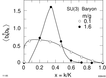
Figure 1: Valence contribution to the baryon structure function in QCD₁₊₁, as a function of the light-cone longitudinal momentum fraction. The gauge group is SU(3), $m$ is the quark mass, and $g$ is the gauge coupling. (From Ref. [4].)

In addition to the spectrum, of course, one obtains the wavefunctions. These allow direct computation of, e.g., structure functions. (We shall discuss the particularly close relation between the LC wavefunctions and physical observables in more detail in the following sections.) As an example, Fig. 1 shows the valence contribution to the structure function for an SU(3) baryon, for two values of the dimensionless coupling $m/g$. As expected, for weak coupling the distribution is peaked near $x=1/3$, reflecting that the baryon momentum is shared essentially equally among its constituents. For comparison, the contributions from Fock states with one and two additional $q\bar{q}$ pairs are shown in Fig. 2. Note that the amplitudes for these higher Fock components are quite small relative to the valence configuration. The lightest hadrons are nearly always dominated by the valence Fock state in these super-renormalizable models; higher Fock wavefunctions are typically suppressed by factors of 100 or more. Thus the light-cone quarks are much more like constituent quarks in these theories than equal-time quarks would be. As discussed above, in an equal-time formulation even the vacuum state would be an infinite superposition of Fock states. Identifying constituents in this case, three of which could account for most of the structure of a baryon, would be quite difficult.

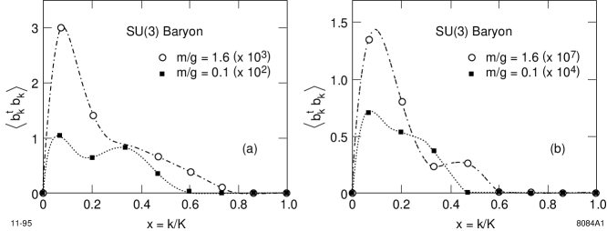
Figure 2: Contributions to the baryon structure function from higher Fock components: (a) valence plus one additional $q\bar{q}$ pair; (b) valence plus two additional $q\bar{q}$ pairs. (From Ref. [4].)

2.3 Problems and Open Issues

In this section we briefly survey the main obstacles to progress in realistic field theories, specifically QCD. These may be grouped into three broad categories: the renormalization problem, the closely related problem of vacuum structure in the LC representation, and the development of practical algorithms for calculations in (3+1)-dimensional theories of interest.

2.3.1 Renormalization

All nontrivial quantum field theories are afflicted with divergences, and LC theories are no exception to this. The theory must first be made finite by introducing a regulator, and then the dependence on the unphysical parameters that characterize the regulator (generically called cutoffs) must be removed by suitably chosen counterterms. These two problems are of course linked, as the counterterms required in general depend strongly on the regulator used. In particular, it is desirable for a regulator to respect as many symmetries as possible, so that counterterms will be restricted to invariant operators.

It is useful to distinguish three generic types of cutoff that are necessary for LC field theory:

• A cutoff on light-cone energies: ${p_{\perp}^{2}+m^{2}\over p^{+}}<\Lambda$

• For massless particles, a cutoff on small longitudinal momenta: $p^{+}>\lambda$

• A possible cutoff on particle number: $n<\nu$

All of these remove high-energy states on the LC, so that their counterterms will be local in LC time.

There are two main difficulties that arise in the determination of these counterterms. First, all known regulators that are nonperturbative and applicable to Hamiltonians violate Lorentz and gauge invariance. That this will generically be the case can be seen by noting that some subset of the Lorentz generators are dynamical, and thus mix states of different particle number. Any truncation that limits particle number will in general violate these symmetries. Gauge invariance will be broken for essentially the same reason; in QED, for example, the Ward identity relates Green functions that involve intermediate states with different particle content. This means that the counterterms themselves must also violate these symmetries, so that physical quantities computed from the full Hamiltonian can be Lorentz- and gauge-invariant. This is a major complication, as it drastically increases the number of possible operators that can occur.

The other main complication follows from the structure of the dispersion relation on the LC [Eq. (8)]. Transverse UV divergences ($p_{\perp}\rightarrow\infty$) can occur for any value of $p^{+}$. This means that counterterms for these divergences in general involve functions of ratios of all available longitudinal momenta. An analogous result holds also for small-$p^{+}$ divergences—they can occur for any $p_{\perp}$, and so counterterms for these will involve functions of transverse momenta. Thus there are in general an infinite number of possible counterterms, even if we restrict consideration to relevant or marginal operators (in the sense of the renormalization group). These problems indicate that renormalization in LC field theory is significantly more complicated than in other formulations. It is here that the familiar “Law of Conservation of Difficulty” asserts itself.

The simplest approach to renormalization is to just compute the counterterms perturbatively. In analogy with improved lattice actions, the idea is that asymptotic freedom should make this sensible if the cutoff is sufficiently high. This is potentially correct for states that are removed by the cutoff $\Lambda$; the perturbative beta function that controls the dependence of the effective coupling on $\Lambda$ is negative for QCD. A perturbative treatment is probably not sufficient for removing dependence on $\lambda,$ however, except perhaps in certain limited domains. One sign that the infrared cutoff is fundamentally different from $\Lambda$ is that longitudinal momentum rescalings are a Lorentz boost, and so must be an exact symmetry of the theory. There can be no beta function associated with longitudinal scale transformations, unlike rescalings in the transverse directions. A more physical point is that all of the vacuum structure is removed by the cutoff $\lambda$. It is very unlikely that the physics associated with the QCD vacuum can be recreated in the form of counterterms using only perturbation theory.

For problems where the structure of the vacuum does not play a central role, however, such a perturbative treatment might be quite useful. For example, in the study of heavy quarkonia one presumably does not have to have complete control over the vacuum (e.g., a nearly massless pion and linear long-range potentials) in order to obtain reasonable results.

A more ambitious approach to the renormalization problem makes use of Wilson’s formulation of the renormalization group (RG) [40, 11]. Here one studies sequences of Hamiltonians that are obtained by iterating a RG transformation which lowers the various cutoffs. The idea is to search for those trajectories of Hamiltonians that can be infinitely long. A Hamiltonian that lies on such a trajectory will give results that are equivalent to a Hamiltonian with infinite cutoffs, that is, results that are cutoff-independent. With a perturbative implementation of the RG this method is equivalent to the first. It is clearly of interest to develop nonperturbative realizations of the RG for use in LC field theories.

2.3.2 The Vacuum

The problem of how to incorporate a nontrivial vacuum in LCQ is closely related to the renormalization problem; all of the structure of the vacuum is removed by a small-$p^{+}$ cutoff, and putting this physics back is one purpose of the infrared counterterms. We prefer to consider it separately, however, because conceptually it is a much different problem than that of removing dependence on a transverse momentum cutoff. The vacuum problem is in fact one aspect of a whole range of puzzles regarding LC field theory, which can all be traced to the fact that the LC initial-value surface contains points that are light-like separated.

Mathematically, the subtleties arise because the LC initial-value surface is a surface of characteristics [41]. Physically, they arise because points on the surface can be causally connected. Thus one may not be completely free to impose initial conditions on such a surface, for example. Furthermore, there is a danger of missing degrees of freedom; in general, initial conditions on one characteristic surface are not sufficient to determine a general solution to the problem [42, 43]. These difficulties are compounded by the fact that the vacuum lives at a very singular point in the theory. Near $p^{+}=0$ states have diverging free energies, but the density of states and couplings to other states are also singular.

One way of addressing these issues is to carefully treat the LC initial-value problem with an infrared regulator that does not make the vacuum trivial [44, 45]. The idea is to formulate the theory with the vacuum degrees of freedom (sometimes called “zero modes,” though this phrase has several distinct meanings among the experts) present, and then to integrate them out. This is essentially the small-$p^{+}$ part of the renormalization problem discussed above. The goal is to obtain either an effective Hamiltonian for use with a trivial vacuum or an explicit description of the vacuum structure in terms of the LC degrees of freedom.

In the past few years there has been significant progress on understanding the ways in which vacuum structure can be manifest on the LC. A consistent mean-field description of spontaneous symmetry breaking in the $\phi^{4}_{1+1}$ theory has been obtained [46], as well as a better understanding of certain topological properties of gauge theories [47]. McCartor’s operator solution of the Schwinger model on the LC is also instructive [23]. In particular the structure of the $\theta$-vacua, while not trivial, is considerably simpler in the LC representation than in ETQ [48].

2.3.3 Tools for Practical Calculations

In this section we shall briefly sketch several practical tools that are being developed for use in LC field theories, and some of the difficulties associated with them. These are in many ways complimentary; they address different practical or theoretical issues. A judicious combination of them will likely be necessary in an attack on QCD.

Discretized Light-Cone Quantization

One approach to small-$k^{+}$ regularization, which is also convenient for setting up numerical calculations, is that of “discretized” light-cone quantization (DLCQ) [27]. In this method one imposes boundary conditions on the fields in an interval

$$-L\leq x^{-}\leq L\;.$$ (12)

This leads to discrete momenta

$$p^{+}_{n}={n\pi\over L}\;,$$ (13)

where $n=0,2,4,\dots$ for periodic and $n=1,3,5,\dots$ for anti-periodic boundary conditions. The Fock space is thus denumerable, and after imposing, e.g., transverse momentum cutoffs the system is completely finite. It can also be shown that when periodic boundary conditions are allowed, the mode with $n=0$ (the “zero mode”) is generally not a dynamical variable, but rather is a constrained functional of the other, dynamical, modes [49]. This is important because it implies that the only state in the theory with $p^{+}=0$ is the Fock vacuum. DLCQ is therefore a particular way of implementing the infrared cutoff that makes the vacuum trivial. However, one must solve the constraints that determine the zero modes.

Most of the actual LC calculations done to date have employed DLCQ, as it gives a particularly clean numerical implementation. This method has been extremely successful, particularly in 1+1 dimensions. A serious difficulty with applying DLCQ to 3+1 dimensional models is the rapid growth of the number of states as the spacetime dimension is increased. For example, with a single particle type and eight momentum states in each of the longitudinal and transverse directions, there are roughly $6\times 10^{15}$ states. The resulting Hamiltonian is far too large even to be stored on a computer, much less diagonalized.

There are several approaches to the problem of large basis size, some of which involve combining DLCQ with the techniques described below. For example, one can attempt to explicitly “integrate out” some of the states, as in the light-front Tamm-Dancoff approach. An interesting implementation of this idea involves formulating the theory in a small transverse volume, or “pipe” [51]. The modes with $p_{\perp}\neq 0$ are then high-energy modes (the lowest nonzero momentum is $\sim 1/L_{\perp}$), and for QCD these can be integrated out using perturbation theory to obtain an effective Hamiltonian for the remaining $p_{\perp}=0$ modes. Thus the full theory is reduced to an effective (1+1)-dimensional theory, which is easily solved using DLCQ. This is the LC analog of the ET “femto-universe” [52], particularly as exploited by Lüscher and van Baal [53]. The main disadvantage is that the computation of the effective Hamiltonian is only reliable for small ($<1~{}{\rm fm}$) transverse volumes. One might hope to systematically improve this, for example by gradually allowing low-transverse-momentum states into the theory.

Light-Front Tamm-Dancoff

LFTD generically refers to integrating out states (higher Fock components, for example) to obtain an effective Hamiltonian for some reasonably-sized subspace [10, 12]. The resulting Hamiltonian can then be solved using DLCQ or some other appropriate technique. Of course, it is generally not possible to integrate out the higher Fock states explicitly. Instead, one attempts to catalog the operators allowed by the few symmetries that are respected by the regulators [24, 12]. Generally one restricts attention to operators that are relevant or marginal in the RG sense. One then tries to fix the coefficients of these operators by, e.g., demanding that symmetries be restored in physical observables.

The main difficulty with this approach is the large number of possible relevant and marginal operators on the LC. As discussed previously, the regulators we are forced to use violate Lorentz and gauge invariance (although subsets of Lorentz invariance can be maintained). Thus the counterterms are not constrained by these symmetries. Furthermore, power counting in LCQ is complicated by the presence of separate scales in the longitudinal and transverse directions. This leads to the appearance of entire functions of ratios of momenta in the counterterms. These are severe complications, and at present it is not known whether this approach will yield a predictive theory, that is, one that does not require the determination of a large number of parameters from fits to data.

As discussed above, one can use perturbation theory to determine the couplings, although one expects this to be inadequate for small-$p^{+}$ quanta. Ultimately, one would like to address these issues with a nonperturbative formulation of the renormalization group. This is a very challenging problem; there are few examples of nonperturbative RGs in all of physics. Alternatively, one can try to study the effects of the small-$p^{+}$ quanta directly, and so uncover the most important operators induced by their elimination.

The Transverse Lattice

A particularly promising approach to practical calculations involves combining LCQ with the transverse lattice formulation of Bardeen, Pearson, and Rabinovici [54]. Here one discretizes the transverse dimensions $x_{\perp}$, but leaves the longitudinal plane $(x^{+},x^{-})$ continuous. One then writes down a LC Hamiltonian in terms of longitudinal gauge fields and transverse link fields (and any matter fields), and attempts to solve the resulting theory using a combination of LC and Monte Carlo techniques [55].

This formulation is advantageous for several reasons. A subset of gauge invariance (in the transverse directions) can be maintained explicitly, so that the renormalization problem is perhaps more tractable. Furthermore, confinement is manifest for finite lattice spacing. One is therefore already in the “correct” phase of the theory, and the challenge is to show that there is no transition to a deconfining phase as the continuum limit is approached. Finally, it turns out that it is not necessary to diagonalize the entire Hamiltonian to study the lowest states. Diagonalization of a small subset of the Hamiltonian which includes nearest- or next-to-nearest-neighbor transverse interactions is sufficient [57].

The main difficulty so far with this approach is a technical one. For non-Abelian gauge theories the transverse lattice formulation reduces to a (1+1)-dimensional gauged nonlinear sigma model (NLSM) at each transverse site, coupled to their immediate neighbors [54]. Furthermore, these NLSMs are integrable theories, so that their exact solutions are in principle known [58]. The problem is translating the known solutions into a representation suitable for application of the LC techniques. Steps in this direction have been taken by Griffin [57], but a complete solution to the problem is lacking. Given the potential advantages of the transverse lattice for studies of QCD, we consider this to be a very important outstanding problem.

2.4 The Road to QCD

The very successful application of the LC formalism to toy models and QED₃₊₁ is encouraging, but much work remains to be done before a full attack on QCD can begin. There has recently been progress on a variety of problems that are important in this regard. There has been a great deal of work on understanding how vacuum structure is manifested in principle when quantizing on a null plane, and how to extract effective Hamiltonians that capture this structure for use with a simple vacuum state. There has also been progress on formulating renormalization groups for LC field theory, as well as perturbatively constructing LC Hamiltonians for QCD. These exhibit some interesting features, for example the natural appearance of a confining potential [39], and can be expected to be useful in, e.g., studies of heavy quarkonia. Calculations using these Hamiltonians have recently been reported [13].

Future research will likely proceed along the broad pathways discussed above. There is a need for nonperturbative calculations of the effective operators that occur in the Hamiltonian when the vacuum structure is eliminated. This requires either a nonperturbative RG or a nonperturbative solution to the “zero mode” problem. In addition, there are challenging technical and numerical issues that arise in (3+1)-dimensional models—even with a trivial vacuum, QCD is still an enormously complicated many-body problem. The formulation of QCD on a transverse lattice is particularly relevant in this regard, as it offers a hope of bringing the explosive growth of the basis size under control.

3 Measures of Light-Cone Wavefunctions

One of the remarkable simplicities of the LC formalism is the fact that one can write down exact expressions for the spacelike electromagnetic form factors $\langle P+Q|J^{+}|P\rangle$ of any hadrons for any initial or final state helicity. At a fixed light-cone time, the exact Heisenberg current can be identified with the free current $j^{+}$. It is convenient to choose the frame in which $q^{+}=0$ so that $q_{\perp}^{2}$ is $Q^{2}=-q_{\mu}^{2}.$ Since the quark current $j^{+}$ has simple matrix elements between free Fock states, each form factor for a given helicity transition $\lambda\rightarrow\lambda^{\prime}$ can be evaluated from simple overlap integrals of the light-cone wavefunctions [14, 15]:

$$F_{\lambda^{\prime},\lambda}(Q^{2})=\sum_{n}\int\prod d^{2}k_{\perp i}\int{\prod dx_{i}}\overline{\psi}_{n,\lambda^{\prime}}(x_{i},k^{\prime}_{\perp i},\lambda_{i})\psi_{n,\lambda}(x_{i},k_{\perp i},\lambda_{i})\;,$$ (14)

where the integrations are over the unconstrained relative coordinates. The internal transverse momenta of the final state wavefunction are $k^{\prime}_{\perp}=k_{\perp}+(1-x)q_{\perp}$ for the struck quark and $k_{\perp}^{\prime}=k_{\perp}-xq_{\perp}$ for the spectator quarks.

The structure functions of a hadron can be computed from the square integral of its LC wavefunctions [38]. For example, the quark distribution measured in deep inelastic scattering at a given resolution $Q^{2}$ is

$$q(x_{Bj},Q^{2})=\sum_{n}\int^{k_{\perp}^{2}<Q^{2}}\prod d^{2}k_{\perp i}\int{\prod dx_{i}}|\psi_{n}(x_{i},k_{\perp i},\lambda_{i})|^{2}\delta(x_{q}=x_{Bj})\;,$$ (15)

where the struck quark is evaluated with its light-cone fraction equal to the Bjorken variable: $x_{q}=x_{Bj}=Q^{2}/2p\cdot q.$ A summation over all contributing Fock states is required to evaluate the form factors and structure functions.

4 Exclusive Processes and Light-Cone Quantization

A central focus of QCD studies at ELFE will be hadron physics at the amplitude level. Exclusive reactions such as pion electroproduction $\gamma^{*}p\rightarrow np$ are more subtle to analyze than deep inelastic lepton scattering and other leading-twist inclusive reactions since they require the consideration of coherent QCD effects. Nevertheless, there is an extraordinary simplification: In any exclusive reaction where the hadrons are forced to absorb large momentum transfer $Q$, one can isolate the nonperturbative long-distance physics associated with hadron structure from the short-distance quark-gluon hard scattering amplitudes responsible for the dynamical reaction. In essence, to leading order in $1/Q,$ each exclusive reaction $AB\rightarrow CD$ factorizes in the form:

$$T_{AB\rightarrow CD}=\int^{1}_{0}\Pi dx_{i}\phi^{\dagger}_{D}(x_{i},Q)\phi^{\dagger}_{C}(x_{i},Q)\phi_{A}(x_{i},Q)\phi_{B}(x_{i},Q)T_{\rm quark}\;,$$ (16)

where $\phi_{A}(x_{i},Q)=\int^{k_{\perp}^{2}<Q^{2}}\prod d^{2}k_{\perp i}{\prod dx_{i}}\psi_{\rm valence}(x_{i},k_{\perp i},\lambda_{i})$ is the process-independent distribution amplitude—the light-cone wavefunction which describes the coupling of hadron $A$ to its valence quark with longitudinal light-cone momentum fractions $0<x_{i}<1$ at impact separation $b={\cal O}(1/Q)$—and $T_{\rm quark}$ is the amplitude describing the hard scattering of the quarks collinear with the hadrons in the initial state to the quarks which are collinear with the hadrons in the final state. Since the propagators and loop momenta in the hard scattering amplitude $T_{\rm quark}$ are of order $Q$, it can be computed perturbatively in QCD. The dimensional counting rules [59] for form factors and fixed CM scattering angle processes follow from the nominal power-law falloff of $T_{\rm quark}$. The scattering of the quarks all occurs at short distances; thus the hard scattering amplitude only couples to the valence-quarks the hadrons when they are at small relative impact parameter. Remarkably, there are no initial state or final state interaction corrections to factorization to leading order in $1/Q$ because of color coherence; final state color interactions are suppressed. This feature not only insures the validity of the factorization theorem for exclusive processes in QCD, but it also leads to the novel effect of “color transparency” in quasi-elastic nuclear reactions [60, 61].

An essential element of the factorization of high momentum transfer exclusive reactions is universality, i.e., the distribution amplitudes $\phi_{A}(x_{i},Q)$ are unique wavefunctions specific to each hadron. Thus the same wavefunction that controls the meson form factors also controls the formation of the mesons in exclusive decay amplitudes of $B$ mesons such as $B\rightarrow\pi\pi$ at the comparable momenta. The distribution amplitudes obey evolution equations and renormalization group equations; for details, see Ref. [38]. A review of the application of light-cone quantized QCD to exclusive processes is given in Ref. [62].

5 The Effective Charge $\alpha_{V}(Q^{2})$ and Light-Cone Quantization

The heavy quark potential plays a central role in QCD, not only in determining the spectrum and wavefunctions of heavy quarkonium, but also in providing a physical definition of the running coupling for QCD. The heavy quark potential $V(Q^{2})$ is defined as the two-particle irreducible amplitude controlling the scattering of two infinitely heavy test quarks $Q\overline{Q}$ in an overall color-singlet state. Here $Q^{2}=-q^{2}={\vec{q}}^{2}$ is the momentum transfer. The effective charge $\alpha_{V}(Q^{2})$ is then defined through the relation $V(Q^{2})=-4\pi C_{F}\alpha_{V}(Q^{2})/Q^{2}$ where $C_{F}=(N_{c}^{2}-1)/2N_{c}=4/3.$ The running coupling $\alpha_{V}(Q^{2})$ satisfies the usual renormalization group equation, where the first two terms $\beta_{0}$ and $\beta_{1}$ in the perturbation series are universal coefficients independent of the renormalization scheme or choice of effective charge. Thus $\alpha_{V}$ provides a physical expansion parameter for perturbative expansions in PQCD.

By definition, all quark and gluon vacuum polarization contributions are summed into $\alpha_{V}$; the scale $Q$ of $\alpha_{V}(Q^{2})$ that appears in perturbative expansions is thus fixed by the requirement that no terms involving the QCD $\beta$-function appear in the coefficients. Thus expansions in $\alpha_{V}$ are identical to that of conformally invariant QCD. This argument is the basis for BLM scale-fixing and commensurate scale relations, which relate physical observables together without renormalization scale, renormalization scheme, or other ambiguities arising from theoretical conventions.

There has recently been remarkable progress [63] in determining the running coupling $\alpha_{V}(Q^{2})$ from heavy quark lattice gauge theory using as input a measured level splitting in the $\Upsilon$ spectrum. The heavy quark potential can also be determined in a direct way from experiment by measuring $e^{+}e^{-}\to c\bar{c}$ and $e^{+}e^{-}\to b\bar{b}$ at threshold [64]. The cross section at threshold is strongly modified by the QCD Sommerfeld rescattering of the heavy quarks through their Coulombic gluon interactions. The amplitude near threshold is modified by a factor $S(\beta,Q^{2})=x/(1-\exp(-x))$, where $x=C_{F}\alpha_{V}(Q^{2})/\beta$ and $\beta=\sqrt{1-4m_{Q}^{2})/s}$ is the relative velocity between the produced quark and heavy quark. The scale $Q$ reflects the mean exchanged momentum transfer in the Coulomb rescattering. For example, the angular distribution for $e^{+}e^{-}\to Q\overline{Q}$ has the form $1+A(\beta)\cos^{2}\theta_{\rm cm}.$ The anisotropy predicted in QCD for small $\beta$ is then $A={\widetilde{A}}/(1+{\widetilde{A}})$, where

$${\widetilde{A}}={\beta^{2}\over 2}{S(\beta,4m_{Q}^{2}\beta^{2}/e)\over S(\beta,4m_{Q}^{2}\beta^{2})}{1-{4\over\pi}\alpha_{V}(m_{Q}^{2}\exp 7/6)\over 1-{16\over 3\pi}\alpha_{V}(m_{Q}^{2}\exp 3/4)}.$$ (17)

The last factor is due to hard virtual radiative corrections. The anisotropy in $e^{+}e^{-}\to Q\overline{Q}$ will be reflected in the angular distribution of the heavy mesons produced in the corresponding exclusive channels.

The renormalization scheme corresponding to the choice of $\alpha_{V}$ as the coupling is the natural one for analyzing QCD in the light-cone formalism, since it automatically sums all vacuum polarization contributions into the coupling. For example, once one knows the form of $\alpha_{V}(Q^{2}),$ it can be used directly in the light-cone formalism as a means to compute the wavefunctions and spectrum of heavy quark systems. The effects of the light quarks and higher Fock state gluons that renormalize the coupling are already contained in $\alpha_{V}.$

The same coupling can also be used for computing the hard scattering amplitudes that control large momentum transfer exclusive reactions and heavy hadron weak decays. Thus when evaluating $T_{\rm quark}$ the scale appropriate for each appearance of the running coupling $\alpha_{V}$ is the momentum transfer of the corresponding exchanged gluon. This prescription agrees with the BLM procedure. The connection between $\alpha_{V}$ and the usual $\alpha_{\overline{MS}}$ scheme is described in Ref. [65].

6 The Physics of Light-Cone Fock States

The light-cone formalism provides the theoretical framework which allows for a hadron to exist in various Fock configurations. For example, quarkonium states not only have valence $Q\overline{Q}$ components but they also contain $Q\overline{Q}g$ and $Q\overline{Q}gg$ states in which the quark pair is in a color-octet configuration. Similarly, nuclear LC wave functions contain components in which the quarks are not in color-singlet nucleon sub-clusters. In some processes, such as large momentum transfer exclusive reactions, only the valence color-singlet Fock state of the scattering hadrons with small inter-quark impact separation $b_{\perp}={\cal O}(1/Q)$ can couple to the hard scattering amplitude. In reactions in which large numbers of particles are produced, the higher Fock components of the LC wavefunction will be emphasized. The higher particle number Fock states of a hadron containing heavy quarks can be diffractively excited, leading to heavy hadron production in the high momentum fragmentation region of the projectile. In some cases the projectile’s valence quarks can coalesce with quarks produced in the collision, producing unusual leading-particle correlations. Thus the multi-particle nature of the LC wavefunction can manifest itself in a number of novel ways. For example:

Color Transparency

QCD predicts that the Fock components of a hadron with a small color dipole moment can pass through nuclear matter without interactions [60, 61]. Thus in the case of large momentum transfer reactions, where only small-size valence Fock state configurations enter the hard scattering amplitude, both the initial and final state interactions of the hadron states become negligible. There is now evidence for QCD “color transparency” in exclusive virtual photon $\rho$ production for both nuclear coherent and incoherent reactions in the E665 experiment at Fermilab [66], as well as the original measurement at BNL in quasi-elastic $pp$ scattering in nuclei [67]. In contrast to color transparency, Fock states with large-scale color configurations interact strongly and with high particle number production [68].

Hidden Color

The deuteron form factor at high $Q^{2}$ is sensitive to wavefunction configurations where all six quarks overlap within an impact separation $b_{\perp i}<{\cal O}(1/Q);$ the leading power-law falloff predicted by QCD is $F_{d}(Q^{2})=f(\alpha_{s}(Q^{2}))/(Q^{2})^{5}$, where, asymptotically, $f(\alpha_{s}(Q^{2}))\propto\alpha_{s}(Q^{2})^{5+2\gamma}$ [69]. The derivation of the evolution equation for the deuteron distribution amplitude and its leading anomalous dimension $\gamma$ is given in Ref. [70]. In general, the six-quark wavefunction of a deuteron is a mixture of five different color-singlet states. The dominant color configuration at large distances corresponds to the usual proton-neutron bound state. However at small impact space separation, all five Fock color-singlet components eventually acquire equal weight, i.e., the deuteron wavefunction evolves to 80% “hidden color.” The relatively large normalization of the deuteron form factor observed at large $Q^{2}$ points to sizable hidden color contributions [71].

Spin-Spin Correlations in Nucleon-Nucleon Scattering and the Charm Threshold

One of the most striking anomalies in elastic proton-proton scattering is the large spin correlation $A_{NN}$ observed at large angles [72]. At $\sqrt{s}\simeq 5$ GeV, the rate for scattering with incident proton spins parallel and normal to the scattering plane is four times larger than that for scattering with antiparallel polarization. This strong polarization correlation can be attributed to the onset of charm production in the intermediate state at this energy [73]. The intermediate state $|uuduudc\bar{c}\rangle$ has odd intrinsic parity and couples to the $J=S=1$ initial state, thus strongly enhancing scattering when the incident projectile and target protons have their spins parallel and normal to the scattering plane. The charm threshold can also explain the anomalous change in color transparency observed at the same energy in quasi-elastic $pp$ scattering. A crucial test is the observation of open charm production near threshold with a cross section of order of $1\mu$b.

Anomalous Decays of the $J/\psi$

The dominant two-body hadronic decay channel of the $J/\psi$ is $J/\psi\rightarrow\rho\pi$, even though such vector-pseudoscalar final states are forbidden in leading order by helicity conservation in perturbative QCD [74]. The $\psi^{\prime}$, on the other hand, appears to respect PQCD. The $J/\psi$ anomaly may signal mixing with vector gluonia or other exotica [74].

The QCD Van Der Waals Potential and Nuclear Bound Quarkonium

The simplest manifestation of the nuclear force is the interaction between two heavy quarkonium states, such as the $\Upsilon(b\bar{b})$ and the $J/\psi(c\bar{c})$. Since there are no valence quarks in common, the dominant color-singlet interaction arises simply from the exchange of two or more gluons. In principle, one could measure the interactions of such systems by producing pairs of quarkonia in high energy hadron collisions. The same fundamental QCD van der Waals potential also dominates the interactions of heavy quarkonia with ordinary hadrons and nuclei. As shown in Ref. [75], the small size of the $Q\overline{Q}$ bound state relative to the much larger hadron allows a systematic expansion of the gluonic potential using the operator product expansion. The coupling of the scalar part of the interaction to large-size hadrons is rigorously normalized to the mass of the state via the trace anomaly. This scalar attractive potential dominates the interactions at low relative velocity. In this way one establishes that the nuclear force between heavy quarkonia and ordinary nuclei is attractive and sufficiently strong to produce nuclear-bound quarkonium [75, 76].

Anomalous Quarkonium Production at the Tevatron

Strong discrepancies between conventional QCD predictions and experiment of a factor of 30 or more have recently been observed for $\psi$, $\psi^{\prime}$, and $\Upsilon$ production at large $p_{T}$ in high energy $p\overline{p}$ collisions at the Tevatron [77]. Braaten and Fleming [78] have suggested that the surplus of charmonium production is due to the enhanced fragmentation of gluon jets coupling to the octet $c\overline{c}$ components in higher Fock states $|c\overline{c}gg\rangle$ of the charmonium wavefunction. Such Fock states are required for a consistent treatment of the radiative corrections to the hadronic decay of $P$-waves in QCD [79].

Intrinsic Heavy Quark Contributions in Hadron Wavefunctions

As we have emphasized, the QCD wavefunction of a hadron can be represented as a superposition of quark and gluon light-cone Fock states: $|\Psi_{\pi^{-}}\rangle=\sum_{n}\psi_{n/\pi^{-}}(x_{i},k_{\perp i},\lambda_{i})|n\rangle$, where the color-singlet states $|n\rangle$ represent the Fock components $|\overline{u}d\rangle$, $|\overline{u}dg\rangle$, $|\overline{u}dQ\overline{Q}\rangle$, etc. Microscopically, the intrinsic heavy-quark Fock component in the $\pi^{-}$ wavefunction, $|\overline{u}dQ\overline{Q}\rangle$, is generated by virtual interactions such as $gg\rightarrow Q\overline{Q}$ where the gluons couple to two or more projectile valence quarks. The probability for $Q\overline{Q}$ fluctuations to exist in a light hadron thus scales as $\alpha_{s}^{2}(m_{Q}^{2})/m_{Q}^{2}$ relative to leading-twist production [80]. This contribution is therefore higher twist, and power-law suppressed compared to sea quark contributions generated by gluon splitting. When the projectile scatters in the target, the coherence of the Fock components is broken and its fluctuations can hadronize, forming new hadronic systems from the fluctuations [16]. For example, intrinsic $c\overline{c}$ fluctuations can be liberated provided the system is probed during the characteristic time $\Delta t=2p_{\rm lab}/M^{2}_{c\overline{c}}$ that such fluctuations exist. For soft interactions at momentum scale $\mu$, the intrinsic heavy quark cross section is suppressed by an additional resolving factor $\propto\mu^{2}/m^{2}_{Q}$ [81]. The nuclear dependence arising from the manifestation of intrinsic charm is expected to be $\sigma_{A}\approx\sigma_{N}A^{2/3}$, characteristic of soft interactions.

In general, the dominant Fock state configurations are not far off shell and thus have minimal invariant mass ${\cal M}^{2}=\sum_{i}m_{T,i}^{2}/x_{i}$ where $m_{T,i}$ is the transverse mass of the $i^{\rm th}$ particle in the configuration. Intrinsic $Q\overline{Q}$ Fock components with minimum invariant mass correspond to configurations with equal-rapidity constituents. Thus, unlike sea quarks generated from a single parton, intrinsic heavy quarks tend to carry a larger fraction of the parent momentum than do the light quarks [82]. In fact, if the intrinsic $Q\overline{Q}$ pair coalesces into a quarkonium state, the momentum of the two heavy quarks is combined so that the quarkonium state will carry a significant fraction of the projectile momentum.

There is substantial evidence for the existence of intrinsic $c\overline{c}$ fluctuations in the wavefunctions of light hadrons. For example, the charm structure function of the proton measured by EMC is significantly larger than that predicted by photon-gluon fusion at large $x_{Bj}$ [83]. Leading charm production in $\pi N$ and hyperon-$N$ collisions also requires a charm source beyond leading twist [80, 84]. The NA3 experiment has also shown that the single $J/\psi$ cross section at large $x_{F}$ is greater than expected from $gg$ and $q\overline{q}$ production [85]. The nuclear dependence of this forward component is diffractive-like, as expected from the BHMT mechanism. In addition, intrinsic charm may account for the anomalous longitudinal polarization of the $J/\psi$ at large $x_{F}$ seen in $\pi N\rightarrow J/\psi X$ interactions [86].

Further theoretical work is needed to establish that the data on direct $J/\psi$ and $\chi_{1}$ production can indeed be described using a higher-twist intrinsic charm mechanism, as discussed in Ref. [16]. Experimentally, it is important to check whether the $J/\psi$’s produced indirectly via $\chi_{2}$ decay are transversely polarized. This would show that $\chi_{2}$ production is dominantly leading twist. Better data on real or virtual photoproduction of the individual charmonium states would also add important information.

Double Quarkonium Hadroproduction

It is quite rare for two charmonium states to be produced in the same hadronic collision. However, the NA3 collaboration has measured a double $J/\psi$ production rate significantly above background in multi-muon events with $\pi^{-}$ beams at laboratory momentum 150 and 280 GeV/c and a 400 GeV/c proton beam [87]. The relative double to single rate, $\sigma_{\psi\psi}/\sigma_{\psi}$, is $(3\pm 1)\times 10^{-4}$ for pion-induced production, where $\sigma_{\psi}$ is the integrated single $\psi$ production cross section. A particularly surprising feature of the NA3 $\pi^{-}N\rightarrow\psi\psi X$ events is that the laboratory fraction of the projectile momentum carried by the $\psi\psi$ pair is always very large, $x_{\psi\psi}\geq 0.6$ at 150 GeV/c and $x_{\psi\psi}\geq 0.4$ at 280 GeV/c. In some events, nearly all of the projectile momentum is carried by the $\psi\psi$ system! In contrast, perturbative $gg$ and $q\overline{q}$ fusion processes are expected to produce central $\psi\psi$ pairs, centered around the mean value, $\langle x_{\psi\psi}\rangle\approx$ 0.4–0.5, in the laboratory. There have been attempts to explain the NA3 data within conventional leading-twist QCD. Charmonium pairs can be produced by a variety of QCD processes including $B\overline{B}$ production and decay, $B\overline{B}\rightarrow\psi\psi X$ and ${\cal O}(\alpha_{s}^{4})$ $\psi\psi$ production via $gg$ fusion and $q\overline{q}$ annihilation [88, 89]. Li and Liu have also considered the possibility that a $2^{++}c\overline{c}c\overline{c}$ resonance is produced, which then decays into correlated $\psi\psi$ pairs [90]. All of these models predict centrally produced $\psi\psi$ pairs [91, 89], in contradiction to the $\pi^{-}$ data.

Over a sufficiently short time, the pion can contain Fock states of arbitrary complexity. For example, two intrinsic $c\overline{c}$ pairs may appear simultaneously in the quantum fluctuations of the projectile wavefunction and then, freed in an energetic interaction, coalesce to form a pair of $\psi$’s. In the simplest analysis, one assumes the light-cone Fock state wavefunction is approximately constant up to the energy denominator [80]. The predicted $\psi\psi$ pair distributions from the intrinsic charm model provide a natural explanation of the strong forward production of double $J/\psi$ hadroproduction, and thus gives strong phenomenological support for the presence of intrinsic heavy quark states in hadrons.

It is clearly important for the double $J/\psi$ measurements to be repeated with higher statistics and at higher energies. The same intrinsic Fock states will also lead to the production of multi-charmed baryons in the proton fragmentation region. The intrinsic heavy quark model can also be used to predict the features of heavier quarkonium hadroproduction, such as $\Upsilon\Upsilon$, $\Upsilon\psi$, and $(c\bar{b})$ $(\bar{c}b)$ pairs. It is also interesting to study the correlations of the heavy quarkonium pairs to search for possible new four-quark bound states and final state interactions generated by multiple gluon exchange [90], since the QCD Van der Waals interactions could be anomalously strong at low relative rapidity [75, 76].

Leading Particle Effect in Open Charm Production

According to PQCD factorization, the fragmentation of a heavy quark jet is independent of the production process. However, there are strong correlations between the quantum numbers of $D$ mesons and the charge of the incident pion beam in $\pi N\rightarrow DX$ reactions. This effect can be explained as being due to the coalescence of the produced intrinsic charm quark with co-moving valence quarks. The same higher-twist recombination effect can also account for the suppression of $J/\psi$ and $\Upsilon$ production in nuclear collisions in regions of phase space with high particle density [80].

There are many ways in which the intrinsic heavy quark content of light hadrons can be tested. More measurements of the charm and bottom structure functions at large $x_{F}$ are needed to confirm the EMC data [83]. Charm production in the proton fragmentation region in deep inelastic lepton-proton scattering is sensitive to the hidden charm in the proton wavefunction. The presence of intrinsic heavy quarks in the hadron wavefunction also enhances heavy flavor production in hadronic interactions near threshold. More generally, the intrinsic heavy quark model leads to enhanced open and hidden heavy quark production and leading particle correlations at high $x_{F}$ in hadron collisions, with a distinctive strongly shadowed nuclear dependence characteristic of soft hadronic collisions.

7 Charm Production at ELFE

One of the most important areas of experimental investigation at ELFE will be the production of charm near threshold in electroproduction and photoproduction, e.g., $\gamma^{*}p\to J/\psi p$, $\gamma^{*}p\to D\Lambda_{c}$, etc. These processes are important to study since they provide new insights into production mechanisms in QCD and hadronization in a regime where hard gluon radiation is suppressed. Usually one can rely on the PQCD factorization theorems for hard exclusive and inclusive processes to accurately compute the rates for these processes to leading order in $1/m_{c}$. In the low-energy regime accessed by CEBAF and ELFE, however, there can be significantly modifications to the leading twist QCD predictions:

• The role of intrinsic charm becomes dominant over leading-twist fusion processes near threshold, since the multi-connected intrinsic charm configurations in the higher light-cone Fock state of the proton are more efficient that gluon splitting in producing charm.

• The heavy $c$ and $\bar{c}$ will be produced at low velocities relative to each other and with the spectator quarks from the proton and virtual photon. As is the case of $e^{+}e^{-}\to\bar{c}c$ near threshold, the QCD Coulomb rescattering will give Sommerfeld correction factors $S(\beta,Q^{2})$ which strongly distort the Born predictions for the production amplitudes.

8 Nuclear Effects at ELFE

The shadowing of the nuclear structure function $F_{2}^{A}(x,Q^{2})$ at low $x$ reflects the nuclear dependence of the quark-nucleus cross section $\sigma_{qn}(\hat{s})$ at the corresponding $\hat{s}={\cal O}(\overline{k^{2}_{\perp}}/x)$. Here $\overline{k^{2}_{\perp}}$ is the mean square transverse momentum of the interacting quark. In the case of the longitudinal structure function, however, the leading-twist contribution reflects the interaction of gluons in the nucleus. Thus the study of shadowing as a function of photon polarization can discriminate between the effective quark and gluon cross sections $\sigma_{gN}(\hat{s})$ and $\sigma_{qN}(\hat{s}),$ fundamental aspects of quark and gluon interactions. Such a measurement may be possible at ELFE at high energies.

It is also very interesting to measure the nuclear dependence of totally diffractive vector meson production $d\sigma/dt(\gamma^{*}A\to VA).$ For large photon virtualities (or for heavy vector quarkonium), the small color dipole moment of the vector system implies minimal absorption, i.e., color transparency. Thus, remarkably, QCD predicts that the forward amplitude $\gamma^{*}A\to VA$ at $t\to 0$ is nearly linear in $A$. One is also sensitive to corrections from the nonlinear $A$-dependence of the nearly forward matrix element that couples two gluons to the nucleus, which is closely related to the nuclear dependence of the gluon structure function of the nucleus [92].

The integral of the diffractive cross section over the forward peak is thus predicted to scale approximately as $A^{2}/R_{A}^{2}\sim A^{4/3}.$ A test of this prediction could be carried out at very small $t_{\rm min}$ at HERA, and would provide a striking test of QCD in exclusive nuclear reactions. Evidence for color transparency in quasi-elastic $\rho$ leptoproduction $\gamma^{*}A\to\rho^{0}N(A-1)$ has recently been reported by the E665 experiment at Fermilab [93]. It is of interest to extend the quasi-elastic measurements to lower energy at ELFE.

9 Moments of Nucleons and Nuclei in the Light-Cone Formalism

The use of covariant kinematics leads to a number of striking conclusions for the electromagnetic and weak moments of nucleons and nuclei. For example, magnetic moments cannot be written as the naive sum $\overrightarrow{\mu}=\sum\overrightarrow{\mu}_{i}$ of the magnetic moments of the constituents, except in the nonrelativistic limit where the radius of the bound state is much larger than its Compton scale: $R_{A}M_{A}\gg 1$. The deuteron quadrupole moment is in general nonzero even if the nucleon-nucleon bound state has no $D$-wave component [94]. Such effects are due to the fact that even “static” moments must be computed as transitions between states of different momentum $p^{\mu}$ and $p^{\mu}+q^{\mu}$, with $q^{\mu}\rightarrow 0$. Thus one must construct current matrix elements between boosted states. The Wigner boost generates nontrivial corrections to the current interactions of bound systems [95]. Remarkably, in the case of the deuteron, both the quadrupole and magnetic moments become equal to that of the Standard Model in the limit $M_{d}R_{d}\rightarrow 0.$ In this limit, the three form factors of the deuteron have the same ratios as do those of the $W$ boson in the Standard Model [94].

One can also use light-cone methods to show that the proton’s magnetic moment $\mu_{p}$ and its axial-vector coupling $g_{A}$ have a relationship independent of the specific form of the light-cone wavefunction [96]. At the physical value of the proton radius computed from the slope of the Dirac form factor, $R_{1}=0.76$ fm, one obtains the experimental values for both $\mu_{p}$ and $g_{A}$; the helicity carried by the valence $u$ and $d$ quarks are each reduced by a factor $\simeq 0.75$ relative to their nonrelativistic values. At infinitely small radius $R_{p}M_{p}\rightarrow 0$, $\mu_{p}$ becomes equal to the Dirac moment, as demanded by the Drell-Hearn-Gerasimov sum rule [97, 98]. Another surprising fact is that as $R_{1}\rightarrow 0$ the constituent quark helicities become completely disoriented and $g_{A}\rightarrow 0$.

One can understand the origins of the above universal features even in an effective three-quark light-cone Fock description of the nucleon. In such a model, one assumes that additional degrees of freedom (including zero modes) can be parameterized through an effective potential [38]. After truncation, one could in principle obtain the mass $M$ and light-cone wavefunction of the three-quark bound-states by solving the Hamiltonian eigenvalue problem. It is reasonable to assume that adding more quark and gluonic excitations will only refine this initial approximation [10]. In such a theory the constituent quarks will also acquire effective masses and form factors.

Since we do not have an explicit representation for the effective potential in the light-cone Hamiltonian $P^{-}_{\rm eff}$ for three quarks, we shall proceed by making an Ansatz for the momentum-space structure of the wavefunction $\Psi$. Even without explicit solutions of the Hamiltonian eigenvalue problem, one knows that the helicity and flavor structure of the baryon eigenfunctions will reflect the assumed global SU(6) symmetry and Lorentz invariance of the theory. As we will show below, for a given size of the proton the predictions and interrelations between observables at $Q^{2}=0,$ such as the proton magnetic moment $\mu_{p}$ and its axial coupling $g_{A},$ turn out to be essentially independent of the shape of the wavefunction [96].

The light-cone model given in Ref. [99] provides a framework for representing the general structure of the effective three-quark wavefunctions for baryons. The wavefunction $\Psi$ is constructed as the product of a momentum wavefunction, which is spherically symmetric and invariant under permutations, and a spin-isospin wave function, which is uniquely determined by SU(6)-symmetry requirements. A Wigner-Melosh rotation [100, 101] is applied to the spinors, so that the wavefunction of the proton is an eigenfunction of $J$ and $J_{z}$ in its rest frame [102, 103, 104]. To represent the range of uncertainty in the possible form of the momentum wavefunction, one can choose two simple functions of the invariant mass ${\cal M}$ of the quarks:

$$\psi_{\rm H.O.}({\cal M}^{2}) = N_{\rm H.O.}\exp(-{\cal M}^{2}/2\beta^{2}),$$ (18)

$$\psi_{\rm Power}({\cal M}^{2}) = N_{\rm Power}(1+{\cal M}^{2}/\beta^{2})^{-p}\;,$$ (19)

where $\beta$ sets the characteristic internal momentum scale. Perturbative QCD predicts a nominal power-law fall off at large $k_{\perp}$ corresponding to $p=3.5$ [38]. The Melosh rotation insures that the nucleon has $j=\frac{1}{2}$ in its rest system. It has the matrix representation [101]

$$R_{M}(x_{i},k_{\perp i},m)={m+x_{i}{\cal M}-i\overrightarrow{\sigma}\cdot(\vec{n}\times\vec{k}_{i})\over\sqrt{(m+x_{i}{\cal M})^{2}+k_{\perp i}^{2}}}$$ (20)

with $\vec{n}=(0,0,1)$, and it becomes the unit matrix if the quarks are collinear, $R_{M}(x_{i},0,m)=1.$ Thus the internal transverse momentum dependence of the light-cone wavefunctions also affects its helicity structure [95].

The Dirac and Pauli form factors $F_{1}(Q^{2})$ and $F_{2}(Q^{2})$ of the nucleons are given by the spin-conserving and the spin-flip matrix elements of the vector current $J^{+}_{V}$ (at $Q^{2}=-q^{2}$) [15]

$$F_{1}(Q^{2}) = \langle p+q,\uparrow|J^{+}_{V}|p,\uparrow\rangle,$$ (21)

$$(Q_{1}-iQ_{2})F_{2}(Q^{2}) = -2M\langle p+q,\uparrow|J^{+}_{V}|p,\downarrow\rangle\;.$$ (22)

We then can calculate the anomalous magnetic moment $a=\lim_{Q^{2}\rightarrow 0}F_{2}(Q^{2})$. The same parameters as in Ref. [99] are chosen, namely $m=0.263$ GeV (0.26 GeV) for the up (down) quark masses, $\beta=0.607$ GeV (0.55 GeV) for $\psi_{\rm Power}$ ($\psi_{\rm H.O.}$), and $p=3.5$. The quark currents are taken as elementary currents with Dirac moments ${e_{q}\over 2m_{q}}.$ All of the baryon moments are well-fit if one takes the strange quark mass as 0.38 GeV. With the above values, the proton magnetic moment is 2.81 nuclear magnetons, and the neutron magnetic moment is $-1.66$ nuclear magnetons. (The neutron value can be improved by relaxing the assumption of isospin symmetry.) The radius of the proton is 0.76 fm, i.e., $M_{p}R_{1}=3.63$.

In Fig. 3(a) we show the functional relationship between the anomalous moment $a_{p}$ and its Dirac radius predicted by the three-quark light-cone model. The value of

$$R^{2}_{1}=-6{dF_{1}(Q^{2})\over dQ^{2}}\Bigl{|}_{Q^{2}=0}$$ (23)

is varied by changing $\beta$ in the light-cone wavefunction while keeping the quark mass $m$ fixed. The prediction for the power-law wavefunction $\psi_{\rm Power}$ is given by the broken line; the continuous line represents $\psi_{\rm H.O.}$. Figure 3(a) shows that when one plots the dimensionless observable $a_{p}$ against the dimensionless observable $MR_{1}$ the prediction is essentially independent of the assumed power-law or Gaussian form of the three-quark light-cone wavefunction. Different values of $p>2$ also do not affect the functional dependence of $a_{p}(M_{p}R_{1})$ shown in Fig. 3(a). In this sense the predictions of the three-quark light-cone model relating the $Q^{2}\rightarrow 0$ observables are essentially model-independent. The only parameter controlling the relation between the dimensionless observables in the light-cone three-quark model is $m/M_{p}$ which is set to 0.28. For the physical proton radius $M_{p}R_{1}=3.63$ one obtains the empirical value for $a_{p}=1.79$ (indicated by the dotted lines in Fig. 3(a)).

The prediction for the anomalous moment $a$ can be written analytically as $a=\langle\gamma_{V}\rangle a^{\rm NR}$, where $a^{\rm NR}=2M_{p}/3m$ is the nonrelativistic ($R\rightarrow\infty$) value and $\gamma_{V}$ is given as [105]

$$\gamma_{V}(x_{i},k_{\perp i},m)={3m\over{\cal M}}\left[{(1-x_{3}){\cal M}(m+x_{3}{\cal M})-\vec{k}_{\perp 3}^{2}/2\over(m+x_{3}{\cal M})^{2}+\vec{k}_{\perp 3}^{2}}\right]\;.$$ (24)

The expectation value $\langle\gamma_{V}\rangle$ is evaluated as

$$\langle\gamma_{V}\rangle={\int[d^{3}k]\gamma_{V}|\psi|^{2}\over\int[d^{3}k]|\psi|^{2}}\;.$$ (25)

Let us now take a closer look at the two limits $R\rightarrow\infty$ and $R\rightarrow 0$. In the nonrelativistic limit we let $\beta\rightarrow 0$ and keep the quark mass $m$ and the proton mass $M_{p}$ fixed. In this limit the proton radius $R_{1}\rightarrow\infty$ and $a_{p}\rightarrow 2M_{p}/3m=2.38$, since $\langle\gamma_{V}\rangle\rightarrow 1$. Thus the physical value of the anomalous magnetic moment at the empirical proton radius $M_{p}R_{1}=3.63$ is reduced by 25% from its nonrelativistic value due to relativistic recoil and nonzero $k_{\perp}$.

Figure 3: (a). The anomalous magnetic moment of the proton $a_{p}=F_{2}(0)$ as a function of its Dirac radius $M_{p}R_{1}$ in Compton units. (b). The axial vector coupling of the neutron to proton beta-decay as a function of $M_{p}R_{1}.$ In each figure, the broken line is computed from a wavefunction with power-law falloff and the solid curve is computed from a gaussian wavefunction. The experimental values at the physical proton Dirac radius are indicated by the dotted line. (From Ref. LABEL:bs94.)

To obtain the ultra-relativistic limit we let $\beta\rightarrow\infty$ while keeping $m$ fixed. In this limit the proton becomes pointlike, $M_{p}R_{1}\rightarrow 0$, and the internal transverse momenta $k_{\perp}\rightarrow\infty$. The anomalous magnetic momentum of the proton goes linearly to zero as $a=0.43M_{p}R_{1}$ since $\langle\gamma_{V}\rangle\rightarrow 0$. Indeed, the Drell-Hearn-Gerasimov sum rule [97, 98] demands that the proton magnetic moment become equal to the Dirac moment at small radius. For a spin-${1\over 2}$ system

$$a^{2}={M^{2}\over 2\pi^{2}\alpha}\int_{s_{th}}^{\infty}{ds\over s}\left[\sigma_{P}(s)-\sigma_{A}(s)\right]\;,$$ (26)

where $\sigma_{P(A)}$ is the total photoabsorption cross section with parallel (antiparallel) photon and target spins. If we take the point-like limit, such that the threshold for inelastic excitation becomes infinite while the mass of the system is kept finite, the integral over the photoabsorption cross section vanishes and $a=0$ [15]. In contrast, the anomalous magnetic moment of the proton does not vanish in the nonrelativistic quark model as $R\rightarrow 0$. The nonrelativistic quark model does not reflect the fact that the magnetic moment of a baryon is derived from lepton scattering at nonzero momentum transfer, i.e., the calculation of a magnetic moment requires knowledge of the boosted wavefunction. The Melosh transformation is also essential for deriving the DHG sum rule and low-energy theorems of composite systems [95].

A similar analysis can be performed for the axial-vector coupling measured in neutron decay. The coupling $g_{A}$ is given by the spin-conserving axial current $J_{A}^{+}$ matrix element

$$g_{A}(0)=\langle p,\uparrow|J^{+}_{A}|p,\uparrow\rangle\;.$$ (27)

The value for $g_{A}$ can be written as $g_{A}=\langle\gamma_{A}\rangle g_{A}^{\rm NR}$, with $g_{A}^{\rm NR}$ being the nonrelativistic value of $g_{A}$ and with $\gamma_{A}$ given by [105, 106]

$$\gamma_{A}(x_{i},k_{\perp i},m)={(m+x_{3}{\cal M})^{2}-k_{\perp 3}^{2}\over(m+x_{3}{\cal M})^{2}+k_{\perp 3}^{2}}\;.$$ (28)

In Fig. 3(b) the axial-vector coupling is plotted against the proton radius $M_{p}R_{1}$. The same parameters and the same line representation as in Fig. 3(a) are used. The functional dependence of $g_{A}(M_{p}R_{1})$ is also found to be independent of the assumed wavefunction. At the physical proton radius $M_{p}R_{1}=3.63$, one predicts the value $g_{A}=1.25$ (indicated by the dotted lines in Fig. 3(b)), since $\langle\gamma_{A}\rangle=0.75$. The measured value is $g_{A}=1.2573\pm 0.0028$ [107]. This is a 25% reduction compared to the nonrelativistic SU(6) value $g_{A}=5/3,$ which is only valid for a proton with large radius $R_{1}\gg 1/M_{p}.$ As shown in Ref. [106], the Melosh rotation generated by the internal transverse momentum spoils the usual identification of the $\gamma^{+}\gamma_{5}$ quark current matrix element with the total rest-frame spin projection $s_{z}$, thus resulting in a reduction of $g_{A}$.

Thus, given the empirical values for the proton’s anomalous moment $a_{p}$ and radius $M_{p}R_{1},$ its axial-vector coupling is automatically fixed at the value $g_{A}=1.25.$ This is an essentially model-independent prediction of the three-quark structure of the proton in QCD. The Melosh rotation of the light-cone wavefunction is crucial for reducing the value of the axial coupling from its nonrelativistic value 5/3 to its empirical value. The near equality of the ratios $g_{A}/g_{A}(R_{1}\rightarrow\infty)$ and $a_{p}/a_{p}(R_{1}\rightarrow\infty)$ as a function of the proton radius $R_{1}$ shows the wave-function independence of these quantities. We emphasize that at small proton radius the light-cone model predicts not only a vanishing anomalous moment but also $\lim_{R_{1}\rightarrow 0}g_{A}(M_{p}R_{1})=0$. One can understand this physically: in the zero radius limit the internal transverse momenta become infinite and the quark helicities become completely disoriented. This is in contradiction with chiral models, which suggest that for a zero radius composite baryon one should obtain the chiral symmetry result $g_{A}=1$.

The helicity measures $\Delta u$ and $\Delta d$ of the nucleon each experience the same reduction as does $g_{A}$ due to the Melosh effect. Indeed, the quantity $\Delta q$ is defined by the axial current matrix element

$$\Delta q=\langle p,\uparrow|\bar{q}\gamma^{+}\gamma_{5}q|p,\uparrow\rangle\;,$$ (29)

and the value for $\Delta q$ can be written analytically as $\Delta q=\langle\gamma_{A}\rangle\Delta q^{\rm NR}$, with $\Delta q^{\rm NR}$ being the nonrelativistic or naive value of $\Delta q$ and $\gamma_{A}$ given by Eq. (28).

The light-cone model also predicts that the quark helicity sum $\Delta\Sigma=\Delta u+\Delta d$ vanishes as a function of the proton radius $R_{1}$. Since $\Delta\Sigma$ depends on the proton size, it cannot be identified as the vector sum of the rest-frame constituent spins. As emphasized in Ref. [106], the rest-frame spin sum is not a Lorentz invariant for a composite system. Empirically, one can measure $\Delta q$ from the first moment of the leading-twist polarized structure function $g_{1}(x,Q).$ In the light-cone and parton model descriptions, $\Delta q=\int_{0}^{1}dx[q^{\uparrow}(x)-q^{\downarrow}(x)]$, where $q^{\uparrow}(x)$ and $q^{\downarrow}(x)$ can be interpreted as the probability for finding a quark or antiquark with longitudinal momentum fraction $x$ and polarization parallel or antiparallel to the proton helicity in the proton’s infinite momentum frame [38]. [In the infinite momentum frame there is no distinction between the quark helicity and its spin projection $s_{z}.$] Thus $\Delta q$ refers to the difference of helicities at fixed light-cone time or at infinite momentum; it cannot be identified with $q(s_{z}=+{1\over 2})-q(s_{z}=-{1\over 2}),$ the spin carried by each quark flavor in the proton rest frame in the equal-time formalism.

Thus the usual SU(6) values $\Delta u^{\rm NR}=4/3$ and $\Delta d^{\rm NR}=-1/3$ are only valid predictions for the proton at large $MR_{1}.$ At the physical radius the quark helicities are reduced by the same ratio 0.75 as is $g_{A}/g_{A}^{\rm NR}$ due to the Melosh rotation. Qualitative arguments for such a reduction have been given in Refs. [109, 110]. For $M_{p}R_{1}=3.63,$ the three-quark model predicts $\Delta u=1,$ $\Delta d=-1/4,$ and $\Delta\Sigma=\Delta u+\Delta d=0.75$. Although the gluon contribution $\Delta G=0$ in our model, the general sum rule [111]

$${1\over 2}\Delta\Sigma+\Delta G+L_{z}={1\over 2}$$ (30)

is still satisfied, since the Melosh transformation effectively contributes to $L_{z}$.

Suppose one adds polarized gluons to the three-quark light-cone model. Then the flavor-singlet quark-loop radiative corrections to the gluon propagator will give an anomalous contribution $\delta(\Delta q)=-{\alpha_{s}\over 2\pi}\Delta G$ to each light quark helicity [112]. The predicted value of $g_{A}=\Delta u-\Delta d$ is of course unchanged. For illustration we shall choose ${\alpha_{s}\over 2\pi}\Delta G=0.15$. The gluon-enhanced quark model then gives the values in Table 1, which agree well with the present experimental values. Note that the gluon anomaly contribution to $\Delta s$ has probably been overestimated here due to the large strange quark mass. One could also envision other sources for this shift of $\Delta q$ such as intrinsic flavor [110]. A specific model for the gluon helicity distribution in the nucleon bound state is given in Ref. [17].

Quantity	NR	$3q$	$3q+g$	Experiment
$\Delta u$	${4\over 3}$	1	0.85	$0.83\pm 0.03$
$\Delta d$	$-{1\over 3}$	$-{1\over 4}$	–0.40	$-0.43\pm 0.03$
$\Delta s$	0	0	–0.15	$-0.10\pm 0.03$
$\Delta\Sigma$	1	${3\over 4}$	0.30	$0.31\pm 0.07$

Table 1: Comparison of the quark content of the proton in the nonrelativistic quark model (NR), in the three-quark model ($3q$), in a gluon-enhanced three-quark model ($3q+g$), and with experiment [112].

In the above analysis of the singlet moments, it is assumed that all contributions to the sea quark moments derive from the gluon anomaly contribution $\delta(\Delta q)=-{\alpha_{s}\over 2\pi}\Delta G$. In this case the strange and anti-strange quark distributions will be identical. On the other hand, if the strange quarks derive from the intrinsic structure of the proton, then one would not expect this symmetry. For example, in the intrinsic strangeness wavefunctions, the dominant fluctuations in the nucleon wavefunction are most likely dual to intermediate $\Lambda$-$K$ configurations since they have the lowest off-shell light-cone energy and invariant mass. In this case $s(x)$ and $\bar{s}(x)$ will be different.

The light-cone formalism also has interesting consequences for spin correlations in jet fragmentation. In LEP or SLC one produces $s$ and $\bar{s}$ quarks with opposite helicity. This produces a correlation of the spins of the $\Lambda$ and $\overline{\Lambda}$, each produced with large $z$ in the fragmentation of their respective jet. The $\Lambda$ spin essentially follows the spin of the strange quark since the $ud$ has $J=0$. However, this cannot be a 100% correlation since the $\Lambda$ generally is produced with some transverse momentum relative to the $s$ jet. In fact, from the light-cone analysis of the proton spin, we would expect no more than a 75% correlation since the $\Lambda$ and proton radius should be almost the same. On the other hand if $z=E_{\Lambda}/E_{s}\to 1,$ there can be no wasted energy in transverse momentum. At this point one could have 100% polarization. In fact, the nonvalence Fock states will be suppressed at the extreme kinematics, so there is even more reason to expect complete helicity correlation in the endpoint region.

We can also apply a similar idea to the study of the fragmentation of strange quarks to $\Lambda$s produced in deep inelastic lepton scattering on a proton at ELFE. One could use the correlation between the spin of the target proton and the spin of the $\Lambda$ to directly measure the strange polarization $\Delta s.$ It is conceivable that any differences between $\Delta s$ and $\Delta\bar{s}$ in the nucleon wavefunction could be distinguished by measuring the correlations between the target polarization and the $\Lambda$ and $\overline{\Lambda}$ polarization in deep inelastic lepton proton collisions at ELFE or in the target polarization region in hadron-proton collisions.

In summary, we have shown that relativistic effects are crucial for understanding the spin structure of nucleons. By plotting dimensionless observables against dimensionless observables, we obtain relations that are independent of the momentum-space form of the three-quark light-cone wavefunctions. For example, the value of $g_{A}\simeq 1.25$ is correctly predicted from the empirical value of the proton’s anomalous moment. For the physical proton radius $M_{p}R_{1}=3.63$, the inclusion of the Wigner-Melosh rotation due to the finite relative transverse momenta of the three quarks results in a $\sim 25\%$ reduction of the nonrelativistic predictions for the anomalous magnetic moment, the axial vector coupling, and the quark helicity content of the proton. At zero radius, the quark helicities become completely disoriented because of the large internal momenta, resulting in the vanishing of $g_{A}$ and the total quark helicity $\Delta\Sigma.$

10 Future Directions

The light-cone formalism is a very promising framework for the study of hadronic structure. The fact that it allows a precise definition of the parton model means that the light-cone wavefunctions are the most natural way of encoding hadronic structure. The ability to boost states easily—manifested in the frame-independence of the formalism—is another major advantage. Finally, light-cone quantization offers the best hope for deriving a constituent approximation to hadronic structure from QCD. In any other frame, the need to understand the constituents as quasi-particles makes building a connection to a CQM essentially hopeless.

As we have emphasized in these lectures, the proton is represented in QCD at a given light-cone time $x^{+}=t+z$ as a superposition of quark and gluon Fock states $|uud\rangle,|uudg\rangle,|uudQ\overline{Q}\rangle$, etc. Thus when the proton is expanded on a free quark and gluon basis, it is a fluctuating system of arbitrarily large particle number. The light-cone wavefunctions $\psi_{n}(x_{i},k_{\perp i},\lambda_{i})$ are the probability amplitudes which describe the projections of the proton state on this Hilbert space. The structure functions measured in deep inelastic lepton scattering are directly related to the light-cone $x$ momentum distributions of the quarks and gluons determined by the $|\psi_{n}|^{2}$. Another interesting measure of the proton’s structure involves examining the system of hadrons produced in the proton’s fragmentation region when one quark is removed, i.e., the proton’s “fracture functions” [113]. At HERA, the particles derived from the spectator $\bar{3}_{C}$ system which are intrinsic to the proton’s structure are produced in the proton beam direction with approximately the same rapidity as that of the proton at relatively small transverse momentum [84]. Thus in high-energy $ep$ collisions, the electron resolves the diffractively-excited proton, revealing the correlations of the spectator quarks and gluons in its light-cone Fock components with invariant mass extending up to the energy of the collision.

It is of particular interest to examine the fragmentation of the proton when the electron strikes a light quark and the interacting Fock component is the $|uudc\bar{c}\rangle$ or $|uudb\bar{b}\rangle$ state. These Fock components correspond to intrinsic charm or intrinsic bottom quarks in the proton wavefunction. Since the heavy quarks in the proton bound state have roughly the same rapidity as the proton itself, the intrinsic heavy quarks will appear at large $x_{F}$. One expects heavy quarkonium and also heavy hadrons to be formed from the coalescence of the heavy quark with the valence $u$ and $d$ quarks, since they have nearly the same rapidity. Since the heavy and valence quark momenta combine, these states are preferentially produced with large longitudinal momentum fractions.

A recent analysis by Harris, Smith and Vogt [114] of the excessively large charm structure function of the proton at large $x$ as measured by the EMC collaboration at CERN yields an estimate that the probability $P_{c\bar{c}}$ that the proton contains intrinsic charm Fock states is of the order of 0.6%. In the case of intrinsic bottom, PQCD scaling predicts

$$P_{b\bar{b}}=P_{c\bar{c}}{m^{2}_{\psi}\over m^{2}_{\Upsilon}}{\alpha^{4}_{s}(m_{b})\over\alpha^{4}_{s}(m_{c})}\;,$$ (31)

more than an order of magnitude smaller. If super-partners of the quarks or gluons exist they must also appear in higher Fock states of the proton, such as $|uud~{}{\rm gluino}~{}{\rm gluino}\rangle$. At sufficiently high energies, the diffractive excitation of the proton will produce these intrinsic quarks and gluinos in the proton fragmentation region. Such supersymmetric particles can bind with the valence quarks to produce highly unusual color-singlet hybrid supersymmetric states such as $|uud~{}{\rm gluino}\rangle$ at high $x_{F}.$ The probability that the proton contains intrinsic gluinos or squarks scales with the appropriate color factor and inversely with the heavy particle mass squared relative to the intrinsic charm and bottom probabilities. This probability is directly reflected in the production rate when the hadron is probed at a hard scale $Q$ which is large compared to the virtual mass ${\cal M}$ of the Fock state. At low virtualities, the rate is suppressed by an extra factor of $Q^{2}/{\cal M}^{2}.$ The forward proton fragmentation regime is a challenge to instrument at HERA, but it may be feasible to tag special channels involving neutral hadrons or muons. In the case of the gas jet fixed-target $ep$ collisions at ELFE or HERMES, the target fragments emerge at low velocity and large backward angles, and thus may be accessible to precise measurement.

As we have outlined in these lectures, the light-cone Fock representation of quantum chromodynamics provides both a tool and a language for representing hadrons as fluctuating composites of fundamental quark and gluon degrees of freedom. Light-cone quantization provides an attractive method to compute this structure from first principles in QCD. However, much more progress in theory and in experiment will be needed to fulfill this promise.

Acknowledgements

It is a pleasure to thank the organizers of the ELFE Workshop and Summer School, in particular S. D. Bass, for their efforts and hospitality. S.J.B. also wishes to thank J. Hiller, P. Hoyer, O. Jacob, G. P. Lepage, H. J. Lu, A. Mueller, H.-C. Pauli, S. Pinsky, W.-K. Tang, F. Schlumpf, and R. Vogt for helpful conversations. D.G.R. is grateful to M. Burkardt, K. Hornbostel and R. J. Perry for many valuable discussions and comments on portions of the manuscript. The work of S.J.B. was supported by the Department of Energy, contract No. DE-AC03-76SF00515. D.G.R was supported by the National Science Foundation under Grants Nos. PHY-9203145, PHY-9258270, and PHY-9207889.

References

- [1] P. A. M. Dirac, Rev. Mod. Phys. 21, 392 (1949); S. Weinberg, Phys. Rev. 150, 1313 (1966).
- [2] S. J. Brodsky and H.-C. Pauli, in Recent Aspects of Quantum Fields, H. Mitter and H. Gausterer, Eds., Lecture Notes in Physics, Vol. 396 (Springer-Verlag, 1991), and references therein.
- [3] M. Burkardt, Nucl. Phys. A 504, 762 (1989).
- [4] K. Hornbostel, S. J. Brodsky, and H.-C. Pauli, Phys. Rev. D 41, 3814 (1990).
- [5] K. Demeterfi, I. R. Klebanov, and G. Bhanot, Nucl. Phys. B 418, 15 (1994).
- [6] M. Krautgärtner, H.-C. Pauli, and F. Wölz, Phys. Rev. D 45, 3755 (1992); M. Kaluza and H.-C. Pauli, Phys. Rev. D 45, 2968 (1992).
- [7] J. R. Hiller, S. J. Brodsky, and Y. Okamoto, in progress (1995); J. R. Hiller, in Theory of Hadrons and Light-Front QCD, edited by St. D. Glazek (World Scientific, 1995), and talk presented at the 5th Meeting on Light-Cone Quantization and Nonperturbative QCD, Regensburg, Germany, June 1995.
- [8] M. Burkardt, Phys. Rev. D 49, 5446 (1994).
- [9] L.C.L. Hollenberg and N. S. Witte, Phys. Rev. D 50, 3382 (1994).
- [10] R. J. Perry, A. Harindranath and K. G. Wilson, Phys. Rev. Lett. 65, 2959 (1990).
- [11] R. J. Perry, Ann. Phys. 232, 116 (1994).
- [12] K. G. Wilson, T. S. Walhout, A. Harindranath, W.-M. Zhang, R. J. Perry, and St. D. Glazek, Phys. Rev. D 49, 6720 (1994).
- [13] M. Brisudova, talk presented at the 5th Workshop on Light-Cone QCD, Telluride, CO, August 1995; M. Brisudova and R. J. Perry, manuscript in preparation (1995).
- [14] S. D. Drell and T. M. Yan, Phys. Rev. Lett. 24, 181 (1970).
- [15] S. J. Brodsky and S. D. Drell, Phys. Rev. D 22, 2236 (1980).
- [16] S. J. Brodsky, P. Hoyer, A. H. Mueller, W.-K. Tang, Nucl. Phys. B369, 519 (1992).
- [17] S. J. Brodsky, M. Burkardt, and I. A. Schmidt, Nucl. Phys. B 441, 197 (1994).
- [18] G. P. Lepage, Lectures presented at TASI 93, Boulder, CO, June 1993, hep-lat/9403018.
- [19] See, for example, S.J. Brodsky, G. McCartor, H.-C. Pauli, and S. Pinsky, Particle World 3, 109 (1993); R. J. Perry, Lectures presented at Hadrons 94, Gramado, Brazil (1994), hep-th/9407056; K. G. Wilson and D. G. Robertson, in Theory of Hadrons and Light-Front QCD, edited by St. D. Glazek (World Scientific, 1995), hep-th/9411007; M. Burkardt, to appear in Adv. Nucl. Phys., hep-ph/9505259.
- [20] D. G. Robertson and G. McCartor, Z. Phys. C 53, 661 (1992).
- [21] D. E. Soper, Ph. D. thesis, Stanford University (1971).
- [22] K. Hornbostel, Phys. Rev. D 45, 3781 (1992).
- [23] G. McCartor, Z. Phys. C 52, 611 (1991); ibid. 64, 349 (1994).
- [24] K. G. Wilson, lecture presented at the Aspen Center for Physics, August, 1991.
- [25] R. J. Perry, in [19].
- [26] St. D. Glazek and K. G. Wilson, Phys. Rev. D 48, 5863 (1993); ibid. 49, 4214 (1994).
- [27] H.-C. Pauli and S. J. Brodsky, Phys. Rev. D 32, 1993, 2001 (1985).
- [28] H. Bergknoff, Nucl. Phys. B 122, 215 (1977); T. Eller, H.-C. Pauli, and S. J. Brodsky, Phys. Rev. D 35, 1493 (1987); Y. Mo and R. J. Perry, J. Comp. Phys. 108, 159 (1993); K. Harada, A. Okazaki, and M. Taniguchi, Phys. Rev. D 52, 2429 (1995) and KYUSHU–HET 28, hep-th/9509136.
- [29] A. Harindranath and J. P. Vary, Phys. Rev. D 36, 1064, 1141 (1987); ibid. 37, 3010 (1988).
- [30] S. Dalley and I. R. Klebanov, Phys. Rev. D 47, 2517 (1993); G. Bhanot, K. Demeterfi, and I. R. Klebanov, Phys. Rev. D 48, 4980 (1993); F. Antonuccio and S. Dalley, OUTP–9518P, hep-lat/9505009, and OUTP–9524P, hep-ph/9506456.
- [31] M. Burkardt, Phys. Rev. D 47, 4628 (1993).
- [32] St. D. Glazek, A. Harindranath, S. Pinsky, J. Shigemitsu, and K. G. Wilson, Phys. Rev. D 47, 1599 (1993); P. M. Wort, Phys. Rev. D 47, 608 (1993).
- [33] G. McCartor, talk presented at the 5th Workshop on Light-Cone QCD, Telluride, CO, August 1995.
- [34] D. Kutasov and A. Schwimmer, Nucl. Phys. B 442, 447 (1995).
- [35] G. ’t Hooft, Nucl. Phys. B 75, 461 (1974).
- [36] C. J. Hamer, Nucl. Phys. B 195, 503 (1982).
- [37] G. D. Date, Y. Frishman and J. Sonnenschein, Nucl. Phys. B 283, 365 (1987).
- [38] G. P. Lepage and S. J. Brodsky, Phys. Rev. D 22, 2157 (1980).
- [39] R. J. Perry, in Theory of Hadrons and Light-Front QCD, edited by St. D. Glazek (World Scientific, 1995), hep-th/9411037.
- [40] K. G. Wilson and J. B. Kogut, Phys. Rep. 12, 75 (1974); K. G. Wilson, Rev. Mod. Phys. 47, 773 (1975).
- [41] See, for example, P. J. Steinhardt, Ann. Phys. 128, 425 (1980); T. Heinzl and E. Werner, Z. Phys. C 62, 521 (1994); O. C. Jacob, Phys. Rev. D 50, 5289 (1994), Mod. Phys. Lett. A 9, 3219 (1994).
- [42] G. McCartor, Z. Phys. C 41, 271 (1988).
- [43] N. E. Ligterink and B. L. G. Bakker, Amsterdam University preprint (1993).
- [44] F. Lenz, M. Thies, S. Levit, and K. Yazaki, Ann. Phys. 208, 1 (1991); K. Hornbostel, in [22].
- [45] K. Hornbostel, Ph. D. thesis, Stanford University (1988); D. G. Robertson, talk presented at the 5th Meeting on Light-Cone Quantization and Nonperturbative QCD, Regensburg, Germany, June 1995; K. Hornbostel and D. G. Robertson, manuscript in preparation (1995).
- [46] T. Heinzl, S. Krusche, S. Simbürger, and E. Werner, Z. Phys. C 56, 415 (1992); D. G. Robertson, Phys. Rev. D 47, 2549 (1993); C. M. Bender, S. S. Pinsky, and B. van de Sande, Phys. Rev. D 48, 816 (1993); S. S. Pinsky and B. van de Sande, Phys. Rev. D 49, 2001 (1994); J. Hiller, S. S. Pinsky, and B. van de Sande, Phys. Rev. D 51, 726 (1995). For some earlier work on this problem, see Ref. [29].
- [47] A. C. Kalloniatis, H.-C. Pauli, and S. Pinsky, Phys. Rev. D 50,6633 (1994); A. C. Kalloniatis, MPI–H–V29–1995, hep-th/9509027; S. S. Pinsky and A. C. Kalloniatis, OHSTPY–HEP–TH–95–014, hep-th/95090036.
- [48] G. McCartor, in Theory of Hadrons and Light-Front QCD, edited by St. D. Glazek (World Scientific, 1995), hep-th/9410197.
- [49] T. Maskawa and K. Yamawaki, Prog. Theor. Phys. 56, 270 (1976); V. A. Franke, Yu. A. Novozhilov, and E. V. Prokhvatilov, Lett. Math. Phys. 5, 239, 437 (1981); T. Heinzl, S. Krusche, and E. Werner, Phys. Lett. B 272, 54 (1991); G. McCartor and D. G. Robertson, Z. Phys. C 53, 679 (1992).
- [50] T. Heinzl, S. Krusche, and E. Werner, Phys. Lett. B 256, 55 (1991); A. C. Kalloniatis and H.-C. Pauli, Z. Phys. C 63, 161 (1994); A. C. Kalloniatis and D. G. Robertson, Phys. Rev. D 50, 5262 (1994).
- [51] M. Burkardt, talk presented at the 5th Meeting on Light-Cone Quantization and Nonperturbative QCD, Regensburg, Germany, June 1995; see also Ref. [30], and B. van de Sande and M. Burkardt, MPI–H–V38–1995, hep-th/9510104.
- [52] J. D. Bjorken, in Lectures on Lepton Nucleon Scattering and Quantum Chromodynamics (Birkhäuser, 1982).
- [53] See, for example, M. Lüscher, Nucl. Phys. B 219, 233 (1983); P. van Baal, Nucl. Phys. B 351, 183 (1991).
- [54] W. A. Bardeen and R. B. Pearson, Phys. Rev. D 14, 547 (1976); W. A. Bardeen, R. B. Pearson, and E. Rabinovici, Phys. Rev. D 21, 1037 (1980).
- [55] M. Burkardt, Phys. Rev. D 49, 5446 (1994), and these proceedings.
- [56] J. Kogut and L. Susskind, Phys. Rev. D 11, 395 (1975).
- [57] P. A. Griffin, in Theory of Hadrons and Light-Front QCD, edited by St. D. Glazek (World Scientific, 1995), hep-th/9410243.
- [58] For SU(2) link fields, see: P. Wiegmann, Phys. Lett. B 142, 173 (1984).
- [59] S. J. Brodsky and G. R. Farrar, Phys. Rev. D 11, 1309 (1975).
- [60] G. Bertsch, S. J. Brodsky, A. S. Goldhaber, and J.F. Gunion, Phys. Rev. Lett. 47, 297 (1981).
- [61] S. J. Brodsky and A. H. Mueller, Phys. Lett. B 206, 685 (1988).
- [62] S. J. Brodsky and G. P. Lepage, in Perturbative Quantum Chromodynamics, edited by A. Mueller (World Scientific, Singapore, 1989).
- [63] C. T. H. Davies, K. Hornbostel, G. P. Lepage, A. Lidsey, J. Shigemitsu, and J. Sloan, Phys. Lett. B 345, 42 (1995).
- [64] S. J. Brodsky, A. H. Hoang, J. H. Kühn, and T. Teubner, Phys. Lett. B 359, 355 (1995).
- [65] S. J. Brodsky and H. J. Lu, Phys. Rev. D 51, 3652 (1995).
- [66] G. Fang, et al., (1993), presentation at the INT-Fermilab Workshop Perspectives of High Energy Strong Interaction Physics at Hadron Facilities (1993); M. R. Adams, et al., Phys. Rev. Lett. 74, 1525 (1995).
- [67] S. Heppelmann, Nucl. Phys. B (Proc. Suppl.) 12, 159 (1990), and references therein.
- [68] B. Blaettel, G. Baym, L.L. Frankfurt, H. Heiselberg, M. Strikman, Phys. Rev. D 47, 2761 (1993).
- [69] S. J. Brodsky and B. T. Chertok, Phys. Rev. D 14, 3003 (1976).
- [70] S. J. Brodsky, C.-R. Ji, and G. P. Lepage, Phys. Rev. Lett. 51, 83 (1983).
- [71] G. R. Farrar, K. Huleihel, H. Zhang, Phys. Rev. Lett. 74, 650 (1995).
- [72] A. D. Krisch, Nucl. Phys. B (Proc. Suppl.) 25, 285 (1992).
- [73] S. J. Brodsky and G. F. de Teramond, Phys. Rev. Lett. 60, 1924 (1988).
- [74] S. J. Brodsky, G. P. Lepage, and S. F. Tuan, Phys. Rev. Lett. 59, 621 (1987).
- [75] M. Luke, A. V. Manohar and M. J. Savage, Phys. Lett. B 288, 355 (1992).
- [76] S. J. Brodsky, G. F. de Teramond, and I. A. Schmidt, Phys. Rev. Lett. 64, 1011 (1990).
- [77] CDF Collaboration (F. Abe et al.), FERMILAB-PUB-95-271-E, Aug 1995.
- [78] E. Braaten and S. Fleming, Phys. Rev. Lett. 74, 3327 (1995).
- [79] G. T. Bodwin, E. Braaten, and G. P. Lepage, Phys. Rev. D 51, 1125 (1995).
- [80] R. Vogt and S. J. Brodsky, Nucl. Phys. B 438, 261 (1995).
- [81] S. J. Brodsky, J. C. Collins, S. D. Ellis, J. F. Gunion, and A. H. Mueller, Snowmass Summer Study 1984:227 (QCD184:S7:1984).
- [82] S. J. Brodsky, P. Hoyer, C. Peterson, and N. Sakai, Phys. Lett. B 93, 451 (1980).
- [83] J. J. Aubert, et al., Nucl. Phys. B 123, 1 (1983).
- [84] S. J. Brodsky, W.-K. Tang, and P. Hoyer, SLAC-PUB-95-6858 (1995), to be published in Phys. Rev. D.
- [85] J. Badier, et al., Z. Phys. C 20, 1010 (1983).
- [86] C. Biino, et al., Phys. Rev. Lett. 58, 2523 (1987).
- [87] J. Badier, et al., Phys. Lett B 114, 457 (1982), ibid. 158, 85 (1985).
- [88] R. E. Ecclestone and D. M. Scott, Phys. Lett. B 120, 237 (1983).
- [89] V. G. Kartvelishvili and S. E’sakiya, Sov. J. Nucl. Phys. 38(3), 430 (1983) [Yad. Fiz. 38, 772 (1983)].
- [90] B. A. Li and K. F. Liu, Phys. Rev. D 29, 426 (1984).
- [91] V. Barger, F. Halzen, and W. Y. Keung, Phys. Lett. B 119, 453 (1983).
- [92] S. J. Brodsky, L. Frankfurt, J. F. Gunion, A. H. Mueller, and M. Strikman, Phys. Rev. D 50, 3134 (1994).
- [93] Adams, et al., in [66].
- [94] S. J. Brodsky and J. R. Hiller, Phys. Rev. C 28, 475 (1983).
- [95] S. J. Brodsky and J. R. Primack, Ann. Phys. 52 315 (1969); Phys. Rev. 174, 2071 (1968).
- [96] S. J. Brodsky and F. Schlumpf, Phys. Lett. B 329, 111 (1994).
- [97] S. B. Gerasimov, Yad. Fiz. 2, 598 (1965) [Sov. J. Nucl. Phys. 2, 430 (1966)].
- [98] S. D. Drell and A. C. Hearn, Phys. Rev. Lett. 16, 908 (1966).
- [99] F. Schlumpf, Phys. Rev. D 47, 4114 (1993); Mod. Phys. Lett. A 8, 2135 (1993); Phys. Rev. D 48, 4478 (1993); J. Phys. G 20, 237 (1994).
- [100] E. Wigner, Ann. Math. 40, 149 (1939).
- [101] H. J. Melosh, Phys. Rev. D 9, 1095 (1974); L. A. Kondratyuk and M. V. Terent’ev, Yad. Fiz. 31, 1087 (1980) [Sov. J. Nucl. Phys. 31, 561 (1980)]; D. V. Ahluwalia and M. Sawicki, Phys. Rev. D 47, 5161 (1993).
- [102] L. L. Frankfurt and M. I. Strikman, Nucl. Phys. B 148, 107 (1979), Phys. Rep. 76, 215 (1981); L. A. Kondratyuk and M. I. Strikman, Nucl. Phys. A 426, 575 (1984); L. L. Frankfurt, T. Frederico, and M. Strikman, Phys. Rev. C 48, 2182 (1993).
- [103] F. Coester and W. N. Polyzou, Phys. Rev. D 26, 1349 (1982); P. L. Chung, F. Coester, B. D. Keister and W. N. Polyzou, Phys. Rev. C 37, 2000 (1988).
- [104] H. Leutwyler and J. Stern, Ann. Phys. 112, 94 (1978).
- [105] P. L. Chung and F. Coester, Phys. Rev. D 44, 229 (1991).
- [106] B.-Q. Ma, J. Phys. G. 17, L53 (1991); B.-Q. Ma and Qi-Ren Zhang, Z. Phys. C 58, 479 (1993).
- [107] Particle Data Group, Phys. Rev. D 45 (Part 2), 1 (1992).
- [108] J. Ellis and M. Karliner, Phys. Lett. B 341, 397 (1995).
- [109] G. Karl, Phys. Rev. D 45, 247 (1992).
- [110] H. Fritzsch, Mod. Phys. Lett. A 5, 625 (1990).
- [111] R. L. Jaffe and A. Manohar, Nucl. Phys. B 337, 509 (1990).
- [112] A. V. Efremov and O. V. Teryaev, Proceedings of the International Symposium on Hadron Interactions (Bechyne), eds. J. Fischer, P. Kolar and V. Kundrat (Prague), 302 (1988); G. Altarelli and G. G. Ross, Phys. Lett. B 212, 391 (1988); R. D. Carlitz, J. C. Collins and A. H. Mueller, Phys. Lett. B 214, 229 (1988).
- [113] L. Trentadue and G. Veneziano, Phys. Lett. B 323, 201 (1994).
- [114] B. W. Harris, J. Smith, and R. Vogt, hep-ph/9508403 (1995).