SISSA 102/95/EP

The $\Delta I=1/2$ Selection Rule

V. Antonelli, S. Bertolini, M. Fabbrichesi and E.I. Lashin

INFN, Sezione di Trieste
and
Scuola Internazionale Superiore di Studi Avanzati
via Beirut 4, I-34013 Trieste, Italy.

Abstract

We compute the isospin $I=0$ and 2 amplitudes for the decay of a kaon into two pions by estimating the relevant hadronic matrix elements in the chiral quark model. The results are parametrized in terms of the quark and gluon condensates and of the constituent quark mass $M$. The latter is a parameter characteristic of the model, that we restrict by matching the results in the two $\gamma_{5}$-schemes (HV and NDR) of dimensional regularization. We find that, for values of these parameters within the current determinations, the $\Delta I=1/2$ selection rule is well reproduced by means of the cumulative effects of short-distance NLO Wilson coefficients, penguin diagrams, non-factorizable soft-gluon corrections and meson-loop renormalization.

SISSA 102/95/EP
October 1995

1 Introduction

The $\Delta I=1/2$ selection rule [1] states that, in the weak non-leptonic decays of kaons (as well as of hyperons) the amplitude in which the change in isospin is 3/2 is very suppressed with respect to that in which the change is 1/2.

For the decay of a neutral kaon into two pions, the $CP$-conserving amplitude with a final $I=0$ state ($\Delta I=1/2$) is measured to be [2]

$$\mathop{\mbox{Re}}\,A_{0}(K^{0}\rightarrow 2\pi)=3.33\times 10^{-7}\>\mbox{GeV}\,,$$ (1.1)

and it is approximately 22 times larger than that with the pions in the $I=2$ state ($\Delta I=3/2$):

$$\mathop{\mbox{Re}}\,A_{2}(K^{0}\rightarrow 2\pi)=1.50\times 10^{-8}\>\mbox{GeV}\,.$$ (1.2)

Since a naive estimate of the relevant hadronic matrix elements within the standard model leads to amplitudes that are comparable in size, this selection rule has been a standing puzzle, the solution of which has attracted a great deal of theoretical work over the past 40 years (for a review see, for instance, ref. [3]).

Among the most important steps in the progressive understanding of this selection rule, we mention (without any pretense to completeness) the work of Wilson [4], Gaillard–Lee [5] and Altarelli–Maiani [6] who stressed the importance of QCD short-distance corrections; the contribution of Vainshtein–Zakharov–Shifman [7] who identified in the gluon penguin operators a possible source of enhancement of $A_{0}$ with respect of $A_{2}$, and the subsequent work of various authors [8] who correctly estimated the size of them.

At the same time, a parallel development took place as Cohen–Manhoar [9] first pointed out the relevance for the selection rule of meson-loop corrections in a chiral quark model computation, Bardeen–Buras–Gerard [10] estimated this effect in the $1/N_{c}$ approach with the meson loops regularized by a cutoff and, more recently, Kambor–Missimer–Wyler [11] in chiral perturbation theory.

What is then the present status of the rule?

The two main ingredients entering the theoretical estimate of the selection rule are the perturbative determination of the Wilson coefficients of the relevant operators and the (non-perturbative) evaluation of the hadronic matrix elements.

The short distance part of the analysis can be obtained by a straigthforward (albeit challenging) application of renormalization group equation methods. In this respect, we have only updated existing analyses by including next-to-leading order results [12, 13] and evaluating the Wilson coefficients at various hadronic scales for an updated range of $\Lambda_{\rm QCD}^{(4)}$, as explained in section 1.

Most of the uncertainty resides in the second ingredient: the evaluation of hadronic matrix elements. The vacuum saturation approximation (VSA) is not sufficient—non-factorizable and non-perturbative effects are essential in a dynamical explanation of the rule—and a model for QCD at low energies is called for in order to make a progress in this direction.

In ref. [15] (hereafter referred to as I) we have completed a systematic study of the chiral quark model ($\chi$QM) [16, 17, 18] and derived the complete $O(p^{2})$ $\Delta S=1$ chiral Lagrangian. The model allows us to determine the coefficient of each term of the chiral lagrangian as a function of a few input parameters. All the relevant hadronic matrix elements can accordingly be computed and the study of the $\Delta I=1/2$ rule performed.

The first ingredient that makes the predictions of the $\chi$QM substantially different from the VSA results is the inclusion of corrections of order $O(\alpha_{s}N_{c})$ coming from the non-factorizable gluon condensates, first considered by Pich–de Rafael [19] (see ref. [20] for an updating of this analysis). These are truly non-perturbative effects which represent a crucial step toward the understanding of the selection rule. Their most relevant effect is to give the required suppression of the $A_{2}$ amplitude.

To the amplitudes thus obtained, we have consistently added the renormalization induced by meson loops, that we have computed in I. This gives the needed long-distance enhancement of $A_{0}$ while little affecting $A_{2}$. The meson-loop renormalization also provides the scale dependence of the hadronic matrix elements which is necessary in order to make the matching with the Wilson coefficients consistent.

The idea of matching the scale dependence of the meson renormalization to the short-distance $\mu$-dependence of the Wilson coefficients goes back to the work of Bardeen–Buras–Gerard [10] (and subsequently [21]), who, however, applied it in the framework of a cut-off dependent regularization and therefore with results that are different from ours.

All the relevant matrix elements are given in I, to which we refer. We report in section 3 those that are most important for the present analysis. In section 4 we discuss our results at the varying of $\Lambda_{\rm QCD}$, the matching scale $\mu$ and of the input parameters: gluon and quark condensates. The $\chi$QM leaves us with a free parameter: the constituent quark mass $M$. In order to restrict the possible values it can take, we require, as an additional constraint, that the $\gamma_{5}$-scheme dependence of the hadronic matrix elements compensates maximally that of the Wilson coefficients.

As depicted in fig. 9 of section 5, the combined effects of all contributions thus included add up to provide, to a very good approximation, the experimental values for the $I=0$ and 2 amplitudes. We think that our analysis shows that the $\Delta I=1/2$ selection rule is fully accounted for within the standard model and by our present understanding of its non-perturbative aspects.

This said, a word of caution is perhaps advisable. Various uncertainties related to the input parameters are necessarily present in our computation and we will discuss them as they occur. In addition, we have to consider the approximations inherent to our approach. In particular, higher-order terms $O(p^{4})$ in the chiral expansion may cause a 20-30% correction [22]. This is the systematic uncertainty we ascribe to our results.

2 Effective Quark Lagrangian and NLO Wilson Coefficients

The quark effective lagrangian at a scale $\mu<m_{c}$ can be written as [23]

$${\cal L}_{\Delta S=1}=-\frac{G_{F}}{\sqrt{2}}V_{ud}\,V^{*}_{us}\sum_{i}\Bigl{[}z_{i}(\mu)+\tau y_{i}(\mu)\Bigr{]}Q_{i}(\mu)\,.$$ (2.1)

The $Q_{i}$ are four-quark operators obtained by integrating out in the standard model the vector bosons and the heavy quarks $t,\,b$ and $c$. A convenient and by now standard basis includes the following ten quark operators:

$$\begin{array}[]{rcl}Q_{1}&=&\left(\overline{s}_{\alpha}u_{\beta}\right)_{\rm V-A}\left(\overline{u}_{\beta}d_{\alpha}\right)_{\rm V-A}\,,\\[4.30554pt] Q_{2}&=&\left(\overline{s}u\right)_{\rm V-A}\left(\overline{u}d\right)_{\rm V-A}\,,\\[4.30554pt] Q_{3,5}&=&\left(\overline{s}d\right)_{\rm V-A}\sum_{q}\left(\overline{q}q\right)_{\rm V\mp A}\,,\\[4.30554pt] Q_{4,6}&=&\left(\overline{s}_{\alpha}d_{\beta}\right)_{\rm V-A}\sum_{q}(\overline{q}_{\beta}q_{\alpha})_{\rm V\mp A}\,,\\[4.30554pt] Q_{7,9}&=&\frac{3}{2}\left(\overline{s}d\right)_{\rm V-A}\sum_{q}\hat{e}_{q}\left(\overline{q}q\right)_{\rm V\pm A}\,,\\[4.30554pt] Q_{8,10}&=&\frac{3}{2}\left(\overline{s}_{\alpha}d_{\beta}\right)_{\rm V-A}\sum_{q}\hat{e}_{q}(\overline{q}_{\beta}q_{\alpha})_{\rm V\pm A}\,,\end{array}$$ (2.2)

where $\alpha$, $\beta$ denote color indices ($\alpha,\beta=1,\ldots,N_{c}$) and $\hat{e}_{q}$ are quark charges. Color indices for the color singlet operators are omitted. The subscripts $(V\pm A)$ refer to $\gamma_{\mu}(1\pm\gamma_{5})$. We recall that $Q_{1,2}$ stand for the $W$-induced current–current operators, $Q_{3-6}$ for the QCD penguin operators and $Q_{7-10}$ for the electroweak penguin (and box) ones.

The functions $z_{i}(\mu)$ and $y_{i}(\mu)$ are the Wilson coefficients and $V_{ij}$ the Kobayashi-Maskawa (KM) matrix elements; $\tau=-V_{td}V_{ts}^{*}/V_{ud}V_{us}^{*}$. The numerical values of the Wilson coefficients depend on $\alpha_{s}$. A recent determination [14] at LEP and SLC gives

$$\alpha_{s}(m_{Z})=0.119\pm 0.006\,,$$ (2.3)

which corresponds to

$$\Lambda^{(4)}_{QCD}=350\pm 100\>\mbox{MeV}\,.$$ (2.4)

The range in eq. (2.4) will be used for our numerical estimate of the amplitudes $A_{0}$ and $A_{2}$.

Even though not all the operators in eq. (2.2) are independent, this basis is of particular interest for the present numerical analysis because it is that employed for the calculation of the Wilson coefficients to the NLO order in $\alpha_{s}$ [12, 13].

In tables 1 and 2 we give explicitly the Wilson coefficients of the ten operators at the scale $\mu=1$ GeV and $\mu=0.8$ GeV, respectively, in the naive dimensional regularization (NDR) and ’t Hooft-Veltman (HV) $\gamma_{5}$-schemes. Since $\mathop{\mbox{Re}}\tau=O(10^{-3})$, the $CP$-conserving component of $A_{0}$ and $A_{2}$ are controlled by the coefficients $z_{i}(\mu)$, which do not depend on $m_{t}$.

$\Lambda_{QCD}^{(4)}$	250 MeV		350 MeV		450 MeV
$\alpha_{s}(m_{Z})_{\overline{MS}}$	0.113		0.119		0.125
HV
$z_{1}$	$(0.0320)$	$-0.539$	$(0.0339)$	$-0.683$	$(0.0355)$	$-0.884$
$z_{2}$	$(0.988)$	$1.30$	$(0.987)$	$1.40$	$(0.987)$	$1.56$
$z_{3}$		$0.0060$		$0.0108$		$0.0210$
$z_{4}$		$-0.0142$		$-0.0230$		$-0.0389$
$z_{5}$		$0.0037$		$0.0052$		$0.0068$
$z_{6}$		$-0.0128$		$-0.0204$		$-0.0341$
$z_{7}/\alpha$		$-0.0041$		$-0.0024$		$-0.0012$
$z_{8}/\alpha$		$0.0087$		$0.0140$		$0.0234$
$z_{9}/\alpha$		$0.0016$		$0.0068$		$0.0140$
$z_{10}/\alpha$		$-0.0084$		$-0.0135$		$-0.0223$
NDR
$z_{1}$	$(0.0503)$	$-0.440$	$(0.0533)$	$-0.535$	$(0.0557)$	$-0.644$
$z_{2}$	$(0.982)$	$1.23$	$(0.981)$	$1.30$	$(0.980)$	$1.37$
$z_{3}$		$0.0100$		$0.0161$		$0.0283$
$z_{4}$		$-0.0281$		$-0.0432$		$-0.0703$
$z_{5}$		$0.0067$		$0.0083$		$0.0088$
$z_{6}$		$-0.0281$		$-0.0438$		$-0.0730$
$z_{7}/\alpha$		$0.0039$		$0.0122$		$0.0218$
$z_{8}/\alpha$		$0.0120$		$0.0208$		$0.0378$
$z_{9}/\alpha$		$0.0102$		$0.0223$		$0.0382$
$z_{10}/\alpha$		$-0.0076$		$-0.0116$		$-0.0180$

Table 1: NLO Wilson coefficients at $\mu=1$ GeV in the HV and NDR schemes. The corresponding values at $\mu=m_{W}$ are given in parenthesis ($\alpha=1/128$). In the HV scheme one has $z_{3-10}(m_{c})=0$. The coefficients $z_{i}(\mu)$, relevant for the study of $CP$ conserving amplitudes, do not depend on $m_{t}$.

$\Lambda_{QCD}^{(4)}$	250 MeV		350 MeV		450 MeV
$\alpha_{s}(m_{Z})_{\overline{MS}}$	0.113		0.119		0.125
HV
$z_{1}$	$(0.0320)$	$-0.657$	$(0.0339)$	$-0.910$	$(0.0355)$	$-1.36$
$z_{2}$	$(0.988)$	$1.38$	$(0.987)$	$1.58$	$(0.987)$	$1.96$
$z_{3}$		$0.0137$		$0.0301$		$0.0798$
$z_{4}$		$-0.0292$		$-0.0540$		$-0.115$
$z_{5}$		$0.0070$		$0.0100$		$0.0123$
$z_{6}$		$-0.0275$		$-0.0515$		$-0.112$
$z_{7}/\alpha$		$-0.0055$		$-0.0030$		$-0.0065$
$z_{8}/\alpha$		$0.0198$		$0.0379$		$0.0827$
$z_{9}/\alpha$		$0.0070$		$0.0203$		$0.0415$
$z_{10}/\alpha$		$-0.0181$		$-0.0330$		$-0.0644$
NDR
$z_{1}$	$(0.0503)$	$-0.524$	$(0.0533)$	$-0.663$	$(0.0557)$	$-0.781$
$z_{2}$	$(0.982)$	$1.29$	$(0.981)$	$1.39$	$(0.980)$	$1.48$
$z_{3}$		$0.0180$		$0.0360$		$0.0870$
$z_{4}$		$-0.0471$		$-0.0852$		$-0.182$
$z_{5}$		$0.0085$		$0.0077$		$-0.0129$
$z_{6}$		$-0.0495$		$-0.0947$		$-0.226$
$z_{7}/\alpha$		$0.0073$		$0.0204$		$0.0366$
$z_{8}/\alpha$		$0.0280$		$0.0589$		$0.143$
$z_{9}/\alpha$		$0.0206$		$0.0441$		$0.0779$
$z_{10}/\alpha$		$-0.0159$		$-0.0267$		$-0.0438$

Table 2: Same as in table 1 at $\mu=0.8$ GeV.

3 The Hadronic Matrix Elements

The $\chi$QM allows us to compute hadronic matrix elements by coupling quarks to the chiral Goldstone bosons. The model and the details of the derivation of the matrix elements are discussed in I, to which we refer the interested reader.

The results for the matrix elements

$$\langle Q_{i}\rangle_{0,2}\equiv\langle 2\,\pi\,,I=0,2\,|Q_{i}|K^{0}\rangle$$ (3.1)

are given by the equations (8.13)-(8.48) of I, including all contributions of order $O(N^{2})$, $O(N)$ and $O(\alpha_{s}N)$. We have used dimensional regularization and, in dealing with the $\gamma_{5}$ matrix, we have worked out the analysis in both the HV and the NDR schemes.

For reference, we report here those elements that are most relevant to the present discussion. The contributions to $A_{0}$ and $A_{2}$ of the electroweak penguin operators $Q_{7-10}$ are suppressed by the smallness of their Wilson coefficients.

In the HV scheme we find:

$$\langle Q_{1}\rangle_{0} = \frac{1}{3}X\left[-1+\frac{2}{N_{c}}\left(1-\delta_{\left\langle GG\right\rangle}\right)\right]+a_{0}(Q_{1})$$ (3.2)

$$\langle Q_{1}\rangle_{2} = \frac{\sqrt{2}}{3}X\left[1+\frac{1}{N_{c}}\left(1-\delta_{\left\langle GG\right\rangle}\right)\right]+a_{2}(Q_{1})$$ (3.3)

$$\langle Q_{2}\rangle_{0} = \frac{1}{3}X\left[2-\frac{1}{N_{c}}\left(1-\delta_{\left\langle GG\right\rangle}\right)\right]+a_{0}(Q_{2})$$ (3.4)

$$\langle Q_{2}\rangle_{2} = \frac{\sqrt{2}}{3}X\left[1+\frac{1}{N_{c}}\left(1-\delta_{\left\langle GG\right\rangle}\right)\right]+a_{2}(Q_{2})$$ (3.5)

$$\langle Q_{3}\rangle_{0} = \frac{1}{N_{c}}X\left(1-\delta_{\left\langle GG\right\rangle}\right)+a_{0}(Q_{3})$$ (3.6)

$$\langle Q_{4}\rangle_{0} = X+a_{0}(Q_{4})$$ (3.7)

$$\langle Q_{5}\rangle_{0} = \frac{2}{N_{c}}\,\frac{\langle\bar{q}q\rangle}{Mf_{\pi}^{2}}\,X^{\prime}+a_{0}(Q_{5})$$ (3.8)

$$\langle Q_{6}\rangle_{0} = 2\,\frac{\langle\bar{q}q\rangle}{f_{\pi}^{2}M}\,X^{\prime}+a_{0}(Q_{6})$$ (3.9)

where

$$X\equiv\sqrt{3}f_{\pi}\left(m_{K}^{2}-m_{\pi}^{2}\right)\quad\mbox{and}\quad X^{\prime}\equiv X\left(1-6\ \frac{M^{2}}{\Lambda_{\chi}^{2}}\right)\,.$$ (3.10)

In the NDR:

$$\langle Q_{1}\rangle_{0} = \frac{1}{3}X\left[-1+\frac{2}{N_{c}}\left(1-\delta_{\left\langle GG\right\rangle}\right)\right]+a_{0}(Q_{1})$$ (3.11)

$$\langle Q_{1}\rangle_{2} = \frac{\sqrt{2}}{3}X\left[1+\frac{1}{N_{c}}\left(1-\delta_{\left\langle GG\right\rangle}\right)\right]+a_{2}(Q_{1})$$ (3.12)

$$\langle Q_{2}\rangle_{0} = \frac{1}{3}X\left[2-\frac{1}{N_{c}}\left(1-\delta_{\left\langle GG\right\rangle}\right)\right]+a_{0}(Q_{2})$$ (3.13)

$$\langle Q_{2}\rangle_{2} = \frac{\sqrt{2}}{3}X\left[1+\frac{1}{N_{c}}\left(1-\delta_{\left\langle GG\right\rangle}\right)\right]+a_{2}(Q_{2})$$ (3.14)

$$\langle Q_{3}\rangle_{0} = \frac{1}{N_{c}}\left(X^{\prime}-\delta_{\left\langle GG\right\rangle}X\right)+a_{0}(Q_{3})$$ (3.15)

$$\langle Q_{4}\rangle_{0} = X^{\prime}+a_{0}(Q_{4})$$ (3.16)

$$\langle Q_{5}\rangle_{0} = \frac{2}{N_{c}}\,\frac{\langle\bar{q}q\rangle}{Mf_{\pi}^{2}}\,X^{\prime\prime}+a_{0}(Q_{5})$$ (3.17)

$$\langle Q_{6}\rangle_{0} = 2\,\frac{\langle\bar{q}q\rangle}{f_{\pi}^{2}M}\,X^{\prime\prime}+a_{0}(Q_{6})$$ (3.18)

where

$$X^{\prime\prime}=X\left(1-9\,\frac{M^{2}}{\Lambda_{\chi}^{2}}\right)\,.$$ (3.19)

The function $a_{0,2}(Q_{i})$ represent the one-loop mesonic renormalization of the hadronic elements and they are given in I. They are made of polynomial terms, generally of the order of

$$\frac{m^{2}}{(4\pi f)^{2}}\,,$$ (3.20)

and logarithmic terms of the order of

$$\frac{m^{2}}{(4\pi f)^{2}}\ln\frac{m^{2}_{a}}{m^{2}_{b}}\,,$$ (3.21)

where the masses can be any among $m_{\pi}$, $m_{K}$ and $m_{\eta}$ and $f$ is the pion decay constant in the tree-level chiral lagrangian.

The one-loop renormalization of $f$ is taken into account by replacing $f$ with $f_{1}$ in the tree-level amplitudes, which amounts to replacing $1/f^{3}$ with $1/f^{3}_{\pi}$ multiplied by

$$1+3\ \frac{f_{\pi}-f_{1}}{f_{\pi}}\simeq 1.18\,.$$ (3.22)

The corrections of $O(\alpha_{s}N)$ are important. They are parametrized by the value of the gluonic condensate:

$$\delta_{\langle GG\rangle}=\frac{N_{c}}{2}\frac{\langle\alpha_{s}GG/\pi\rangle}{16\pi^{2}f^{4}}\,.$$ (3.23)

Their most important effect is to reduce the contribution of the operator $Q_{1}$ and $Q_{2}$ to the amplitude $A_{2}$; in fact,

$$A_{2}\approx(z_{1}+z_{2})\left[1+\frac{1}{N_{c}}(1-\delta_{\langle GG\rangle})\right]$$ (3.24)

and by taking $\delta_{\langle GG\rangle}\simeq 3$, which is what we obtain for the central value of the gluon condensate (see eq. (3.26) below) , the correction is large enough to revert the sign of the $1/N_{c}$ term and thus suppress the amplitude.

A relevant contribution to the amplitude $A_{0}$ arises from the gluonic penguins $Q_{5,6}$, whose matrix elements are directly proportional to the value of $\left\langle\bar{q}q\right\rangle$ and are controlled by $M$ through the suppression factors in (3.10) and (3.19), that make the matrix elements larger for smaller values of $M$.

The meson-loop renormalization is sizable. It enhances $A_{0}$ while little affecting $A_{2}$, as it is needed in order to reproduce the experimental values. An important feature of this correction is the additional scale dependence that is introduced in the hadronic matrix elements and that matches to a good approximation that of the Wilson coefficients.

For the purpose of comparison with the existing literature, it is useful to introduce the effective factors

$$B_{i}^{(0,2)}\equiv\frac{\langle Q_{i}\rangle_{0,2}^{\chi{\rm QM}}}{\langle Q_{i}\rangle_{0,2}^{\rm VSA}}\,,$$ (3.25)

that give the ratio between our hadronic matrix elements and those of the VSA. We shall discuss their numerical values in section 4.3.

3.1 Input Parameters

The quark and the gluon condensates are two input parameters of our computation. As discussed in I, their phenomenological determination is a complicated question (they parametrize the genuine non-perturbative part of the computation) and the literature offers different estimates.

We identify the condensates entering our computation with those obtained by fitting the experimental data by means of the QCD sum rules (QCD–SR) or lattice computations. In our discussion we will vary these input parameters within the given bounds and obtain a range of values for the amplitudes we are interested in.

A review of recent determinations of these parameters, together with a justification of the estimated errors, is given in I. Here we only report the ranges that we will explore in our numerical analysis.

For the gluon condensate, we take the scale independent range

$$\langle\frac{\alpha_{s}}{\pi}GG\rangle=(376\pm 47\>\mbox{MeV})^{4}\,,$$ (3.26)

which encompasses the results of recent QCD-SR analysis [24].

For the quark condensate, we consider the range

$$-(200\>\mbox{MeV})^{3}\leq\left\langle\bar{q}q\right\rangle\leq-(280\>\mbox{MeV})^{3}$$ (3.27)

in order to include the central values and the errors of the QCD-SR [25] and lattice estimates [26].

In discussing the scale dependence of our results, it is necessary to include the perturbative running of the quark condensate. This can be done in the QCD-SR approach by using the renormalization-group running masses $\overline{m}_{u}+\overline{m}_{d}$, the value of which is estimated at $\mu=1$ GeV to be [27]

$$\overline{m}_{u}+\overline{m}_{d}=12\pm 2.5\>\mbox{MeV}$$ (3.28)

for $\Lambda^{(3)}_{\rm QCD}=300\pm 150$ MeV. The error in (3.28) reflects changes in the spectral functions. In our numerical estimates, we will take as input values the running masses at 1 GeV given by (3.28). Even though our preferred range of $\Lambda^{(4)}_{\rm QCD}$ in eq. (2.4) corresponds to $\Lambda^{(3)}_{\rm QCD}=400\pm 100\>\mbox{MeV}$, and therefore is not that employed in ref. [27], we feel that we are not making too large an error since the determination in eq. (3.28) is not very sensitive to the choice of $\Lambda_{\rm QCD}$.

By taking the value (3.28), we find for the scale-dependent (and normal-ordered) condensate

$$\left\langle\bar{q}q\right\rangle(\mu)=-\frac{f_{\pi}^{2}m_{\pi}^{2}(1-\delta_{\pi})}{\overline{m}_{u}(\mu)+\overline{m}_{d}(\mu)}\,,$$ (3.29)

corresponding ($\delta_{\pi}$ is a few percent correction) to the numerical values of

$$\left\langle\bar{q}q\right\rangle=-(238\pm 19\>\mbox{MeV})^{3}$$ (3.30)

at 1 GeV and

$$\left\langle\bar{q}q\right\rangle=-(222\pm 19\>\mbox{MeV})^{3}$$ (3.31)

at 0.8 GeV. The error in eqs. (3.30)–(3.31) corresponds to that in (3.28). The central values in eqs. (3.30)–(3.31) are in the lower half of the range (3.27).

4 Computing $A_{0}$ and $A_{2}$

The physics entering the $\Delta I=1/2$ rule involves very different scales and thus different effective theories. As a consequence, any attempt to an explanation must necessarily depends on several parameters.

Our solution has two input parameters, the quark and gluon condensates, as well as a free, model-dependent parameter: the constituent quark mass $M$. In addition, the short-distance part depends on several high-energy parameters like the KM matrix elements and the masses of the heavy quarks.

We include all ten operators (2.2) even though the effect of the electroweak operators is only of a few percents. We proceed step-by-step summarizing our result by means of tables and figures.

4.1 The VSA Approach

First of all, in order to make possible gauging the progress of our computation of the hadronic matrix elements, we report in table 3 the results one would obtain by using the VSA for the evaluation of the hadronic matrix elements.

	$\mu=0.8$ GeV		$\mu=0.9$ GeV		$\mu=1$ GeV
	NDR	HV	NDR	HV	NDR	HV
$A_{0}$	1.11	0.93	0.89	0.77	0.75	0.67
$A_{2}$	3.00	2.76	3.07	2.87	3.13	2.95
$\Delta_{\gamma_{5}}A_{0}$	$18\%$		$15\%$		$12\%$
$\Delta_{\gamma_{5}}A_{2}$	$8\%$		$7\%$		$6\%$
$\Delta_{\mu}A_{0}$	$39\%-33\%$
$\Delta_{\mu}A_{2}$	$4\%-7\%$

Table 3: Matching-scale and $\gamma_{5}$-scheme dependence of $A_{0}$ (in units of $10^{-7}$ GeV) and $A_{2}$ (in units of $10^{-8}$ GeV) in the VSA approach with NLO Wilson coefficients. The amplitudes are computed for $\Lambda^{(4)}_{\rm QCD}$ = 350 MeV and $\left\langle\bar{q}q\right\rangle$ given in eq. (3.29). The two values quoted for the $\mu$-dependence of the amplitudes correspond to the NDR and HV scheme results in the range between 0.8 and 1.0 GeV.

Several comments are in order. At $\mu=0.8$ GeV $\simeq\Lambda_{\chi}$ (that is our preferred matching scale) and both in the NDR and the HV schemes, $A_{0}$ is too small by a factor of three while $A_{2}$ is two times too large. Therefore, the ratio

$$\omega^{-1}\equiv\mathop{\mbox{Re}}A_{0}/\mathop{\mbox{Re}}A_{2}\simeq 3.7\,,$$ (4.1)

is about a factor six smaller than the experimental value $\omega^{-1}=22.2$.

This estimate is done by using the hadronic matrix element for the penguin operators given by the VSA. We have used for the quark condensate the PCAC expression given in eq. (3.29). As we shall see in the following, a larger value for $A_{0}$ can be obtained by using larger values for the quark condensate. A popular choice is

$$\left\langle\bar{q}q\right\rangle(1\mbox{GeV})=\left(-\frac{m_{K}^{2}f_{K}^{2}}{m_{s}(1\mbox{GeV})}\right)^{1/3}\simeq-260\>\mbox{MeV}\,.$$ (4.2)

The literature also offers determinations of the selection rule in which the matching between Wilson coefficients and hadronic matrix elements is done without meson-loop renormalization but at a much lower values of matching (at about 300 MeV, for instance [19]). Such a procedure is no longer justifiable in view of the NLO determination of the Wilson coefficients that shows, for such a low-energy matching, the breaking down of the perturbative expansion.

In table 3 we have defined

$$\Delta_{\mu}A_{i}\equiv 2\>\left|\frac{A_{i}(0.8\>\mbox{GeV})-A_{i}(1.0\>\mbox{GeV})}{A_{i}(0.8\>\mbox{GeV})+A_{i}(1.0\>\mbox{GeV})}\right|\,,$$ (4.3)

as a direct measure of the scale dependence. The scale dependence of $A_{0}$ is rather large, with $\Delta_{\mu}A_{0}$ almost 40% in the NDR scheme. On the other hand, the $A_{2}$’s scale dependence remains within 10%.

The difference between the HV and NDR results is quantified by

$$\Delta_{\gamma_{5}}A_{i}\equiv 2\>\left|\frac{A_{i}^{\rm NDR}-A_{i}^{\rm HV}}{A_{i}^{\rm NDR}+A_{i}^{\rm HV}}\right|\,.$$ (4.4)

Contrary to the scale dependence, the $\gamma_{5}$-scheme dependence is not large for the amplitude $A_{0}$ and $A_{2}$, remaining below 10% and it is not an issue in this paper. It is however very large in other observable quantities like, for instance, $\varepsilon^{\prime}/\varepsilon$ where it reaches in the $1/N_{c}$ approach the 80% level.

Because the VSA hadronic matrix elements depend neither on the scale nor the $\gamma_{5}$-scheme, the dependences in table 3 are a direct measure of those of the Wilson coefficients.

We now turn to the $\chi$QM model determination of the selection rule.

4.2 Matching and scale dependence

In matching the short-distance Wilson coefficients to the hadronic matrix elements, we combine terms that are scale dependent. Ideally, the scale dependence of the Wilson coefficients should compensate against that of the hadronic matrix elements to provide a scale independent result. In practice, within our approximations and for the central value of $\Lambda^{(4)}_{\rm QCD}$, we find that the scale dependence in our matching remains below 20%. In particular, as shown in table 4, the difference in the value of $A_{0}$ between the matching at 1 GeV and that at $0.8$ is about 20% in both the HV and NDR, to be compared with the values given in table 3, where it is about 30%. For $A_{2}$ it is respectively 12 and 1%.

$\Lambda^{(4)}_{\rm QCD}$ = 250 MeV
	$\mu=0.8$ GeV		$\mu=0.9$ GeV		$\mu=1$ GeV
	NDR	HV	NDR	HV	NDR	HV
$A_{0}$	2.31	2.29	2.17	2.15	2.08	2.04
$A_{2}$	1.66	1.56	1.73	1.65	1.80	1.72
$\Delta_{\gamma_{5}}A_{0}$	$<1\%$		$1\%$		$2\%$
$\Delta_{\gamma_{5}}A_{2}$	$6\%$		$5\%$		$5\%$
$\Delta_{\mu}A_{0}$	$10\%-12\%$
$\Delta_{\mu}A_{2}$	$8\%-10\%$
$\Lambda^{(4)}_{\rm QCD}$ = 350 MeV
	$\mu=0.8$ GeV		$\mu=0.9$ GeV		$\mu=1$ GeV
	NDR	HV	NDR	HV	NDR	HV
$A_{0}$	2.97	2.94	2.66	2.61	2.45	2.39
$A_{2}$	1.60	1.46	1.68	1.56	1.75	1.64
$\Delta_{\gamma_{5}}A_{0}$	$1\%$		$2\%$		$2\%$
$\Delta_{\gamma_{5}}A_{2}$	$9\%$		$8\%$		$6\%$
$\Delta_{\mu}A_{0}$	$19\%-20\%$
$\Delta_{\mu}A_{2}$	$9\%-12\%$
$\Lambda^{(4)}_{\rm QCD}$ = 450 MeV
	$\mu=0.8$ GeV		$\mu=0.9$ GeV		$\mu=1$ GeV
	NDR	HV	NDR	HV	NDR	HV
$A_{0}$	4.26	4.17	3.52	3.41	3.06	2.95
$A_{2}$	1.58	1.34	1.64	1.46	1.71	1.55
$\Delta_{\gamma_{5}}A_{0}$	$2\%$		$3\%$		$4\%$
$\Delta_{\gamma_{5}}A_{2}$	$17\%$		$12\%$		$9\%$
$\Delta_{\mu}A_{0}$	$33\%-34\%$
$\Delta_{\mu}A_{2}$	$8\%-15\%$

Table 4: Same as in table 3 in the $\chi$QM approach, for different values of $\Lambda^{(4)}_{\rm QCD}$. We take for the gluon condensate the central value $\left\langle\alpha_{s}GG/\pi\right\rangle$ = (376 MeV)⁴ and for the quark condensate $\left\langle\bar{q}q\right\rangle$ eq. (3.29). The $\gamma_{5}$-scheme stability is optimized at $M$ = 160 MeV.

As expected, the matching dependence is stronger for larger values of $\Lambda_{\rm QCD}$. We take the central value at 350 MeV as our reference value for the discussion.

Thanks to the satisfactory scale independence, we can take the matching at any values between 0.8 and 1 GeV. Yet it is useful to bear in mind that any number quoted in what follows suffers of an intrinsic uncertainty of at least 20% because of the residual scale dependence in the matching itself. We take the matching at 0.8 GeV as the best compromise between the range of validity of the perturbative regime and that of chiral perturbation theory.

We have also verified the consistency of the perturbative expansion in the short-distance regime by comparing leading order and the NLO results for $A_{0}$ and $A_{2}$ at $\mu=0.8$ GeV. The change in $A_{0}$ turns out to be of about 10% and similarly for $A_{2}$. These values confirm that the choice of the matching scale $\mu=0.8$ GeV is well within the perturbative regime of the QCD short-distance analysis.

The values for $A_{0}$ and $A_{2}$ in table 4 should not be compared directly to the experimental values because they correspond to a specific choice for the quark and gluon condensates, as well as of $M$. A more complete discussion of the dependence of the results on the input parameters is presented in section 4.4.

4.3 The $B_{i}$ Factors

For the purpose of comparison with the existing literature, we collect in table 5 the $B_{i}$ factors for the hadronic matrix elements of the operators in eq. (2.2). The values of the $B_{i}$ depend on the scale at which the matrix elements are evaluated, on the input parameters, on $M$, and on the $\gamma_{5}$-scheme; we have given in table 5 a representative example of their size.

Only the first six operators are relevant for our present analysis and we postpone any comment on the electroweak penguin matrix elements when studying $\varepsilon^{\prime}/\varepsilon$.

The values of $B_{1}^{(0)}$ and $B_{2}^{(0)}$ show that the corresponding hadronic matrix elements in the $\chi$QM are, once non-factorizable contributions and meson renormalization have been included, respectively twelve and three times larger than their VSA values. At the same time, $B_{1}^{(2)}$ and $B_{2}^{(2)}$ turn out to be about half of what found in the VSA. These features make it possible for the selection rule to be reproduced in the $\chi$QM.

For comparison, in the $1/N_{c}$ approach of ref. [10], the inclusion of meson-loop renormalization through a cutoff regularization leads, at the scale of 1 GeV, to $B_{1}^{(0)}=5.2$, $B_{2}^{(0)}=2.2$ and $B_{1}^{(2)}=B_{2}^{(2)}=0.55$ (see ref. [28]), a result that is not sufficient to reproduce the $\Delta I=1/2$ rule. The value $B_{1}^{(2)}=B_{2}^{(2)}=0.55$ in both the $\chi$QM (table 5) and the $1/N_{c}$ approaches is remarkable, and yet a numerical coincidence, since the suppression orginates from gluon condensate corrections in the $\chi$QM, whereas it is the effect of the meson loop renormalization (regularized via explicit cut-off) in ref. [10].

The values of the penguin matrix elements $\left\langle Q_{3}\right\rangle$ and $\left\langle Q_{4}\right\rangle$ in the $\chi$QM lead to rather large $B_{i}$ factors. In the case of $Q_{3}$, the $\chi$QM result has the opposite sign of the VSA result and $B_{3}$ is negative. This is the effect of the large non-perturbative gluon correction.

Regarding the gluon penguin operator $Q_{6}$ (and $Q_{5}$), we find that the $\chi$QM gives a result consistent with the VSA (and the $1/N_{c}$ approach), $B_{6}$ ($B_{5}$) being approximately equal to two for small values of the quark condensate and one at larger values. It is the quadratic dependence (to be contrasted to the linear dependence in the $\chi$QM) of the VSA matrix element for the penguin operators that it responsible for the different weight of these operators at different values of the quark condensate. The lattice estimate for these operators gives $B_{5}=B_{6}=1.0\pm 0.2$ [29].

	HV		NDR
	$\mu=0.8$ GeV	$\mu=1.0$ GeV	$\mu=0.8$ GeV	$\mu=1.0$ GeV
$B^{(0)}_{1}$	10.6	11.1	10.6	11.1
$B^{(0)}_{2}$	2.8	3.0	2.8	3.0
$B^{(2)}_{1}$	0.52	0.55	0.52	0.55
$B^{(2)}_{2}$	0.52	0.55	0.52	0.55
$B_{3}$	$-2.9$	$-3.0$	$-3.4$	$-3.6$
$B_{4}$	1.8	1.9	1.3	1.4
$B_{5}=B_{6}$	$2.6\div 0.93$	$2.7\div 0.98$	$2.0\div 0.74$	$2.2\div 0.78$
$B_{7}^{(0)}$	$3.2\div 2.3$	$3.4\div 2.4$	$3.0\div 2.2$	$3.3\div 2.4$
$B_{8}^{(0)}$	$3.5\div 2.3$	$3.8\div 2.5$	$3.3\div 2.2$	$3.6\div 2.4$
$B_{9}^{(0)}$	3.9	4.0	3.6	3.8
$B_{10}^{(0)}$	4.4	4.7	5.2	5.5
$B_{7}^{(2)}$	$2.6\div 1.4$	$2.8\div 1.5$	$2.6\div 1.4$	$2.8\div 1.5$
$B_{8}^{(2)}$	$2.1\div 1.4$	$2.2\div 1.5$	$2.0\div 1.4$	$2.2\div 1.4$
$B_{9}^{(2)}$	0.52	0.55	0.52	0.55
$B_{10}^{(2)}$	0.52	0.55	0.52	0.55

Table 5: The $B_{i}$ factors in the $\chi$QM (including meson-loop renormalizations) at two different scales: $\mu$ = 0.8 and 1.0 GeV. We have taken the gluon condensate at the central value of eq. (3.26), while the ranges given for $B_{5-8}$ correspond to varying the quark condensate according to eq. (3.27). The results shown are given in the HV and NDR schemes for $M=180$ MeV.

4.4 Dependence on the Input Parameters

In this section we study the dependence of $A_{0}$ and $A_{2}$ on the quark and gluon condensates. Figs. 1, 2, 3 and 4 show such a dependence for $\Lambda_{\rm QCD}^{(4)}=350$ MeV and four representative values of $M$.

Each figure contains the HV result (black lines) as well as the NDR one (grey lines). The spread between these two determinations is mostly due to $A_{2}$ that contains an irreducible $\gamma_{5}$-scheme dependence, as explained in section 4.5.

The gluon condensate dependence is represented by the three horizontal bands, the central one corresponding to the central value given in eq. (3.26), while the other two bound the one standard deviation range. A larger gluon condensate leads to lower values of $A_{2}$.

The dependence on the quark condensate is represented by the points on a given line. The lenght of the lines corresponds to the range given in eq. (3.27).

Larger values of $A_{0}$ are obtained for larger values of the quark condensate and smaller values of $M$. This is the effect of the gluon penguin operators $Q_{5,6}$, whose matrix elements are proportional to the factor

$$\left\langle\bar{q}q\right\rangle\left(1-6\,\frac{M^{2}}{\Lambda_{\chi}^{2}}\right)$$ (4.5)

in the HV scheme, and similarly (with 6 being replaced by 9) in the NDR scheme.

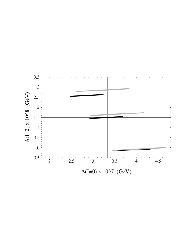
Figure 1: Dependence of $A_{0}$ and $A_{2}$ on $\left\langle\bar{q}q\right\rangle$ and $\left\langle GG\right\rangle$ for $\Lambda^{(4)}_{\rm QCD}=0.350$ GeV, $\mu=0.8$ GeV, and $M=160$ MeV. The black (grey) lines represent the HV (NDR) results by varying $\left\langle\bar{q}q\right\rangle$ in the range of eq. (3.27) for fixed $\left\langle\alpha_{s}GG/\pi\right\rangle$. The three bands correspond to varying $\left\langle\alpha_{s}GG/\pi\right\rangle$ in the range of eq. (3.26), with central lines correponding to the central value of $\left\langle GG\right\rangle$. The experimental values of $A_{0}$ and $A_{2}$ are given by the cross hairs. The small dependence of $A_{2}$ on the quark condensate is due to the the contribution of the electroweak penguins $Q_{7,8}$ .

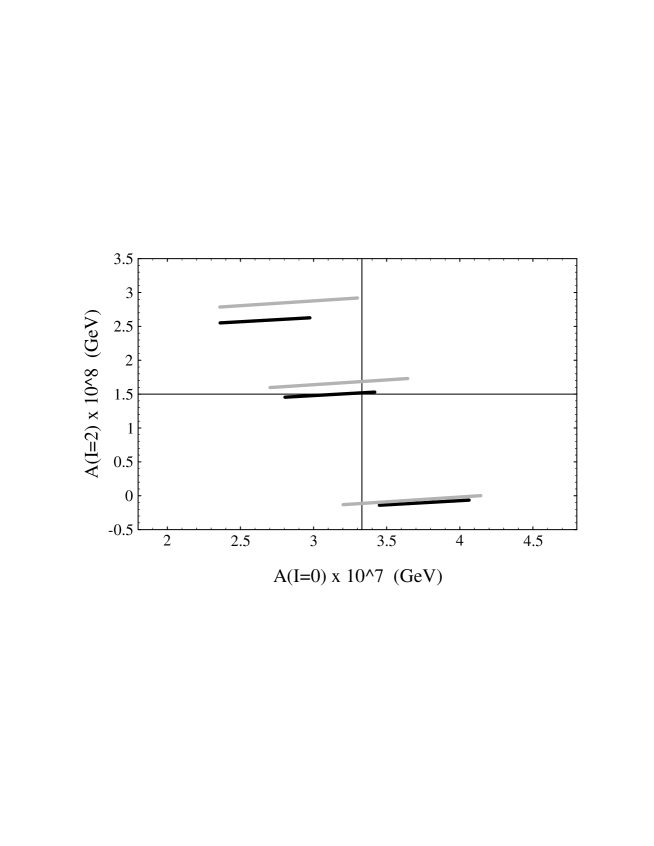
Figure 2: Same as in fig. 1 for $M=180$ MeV.

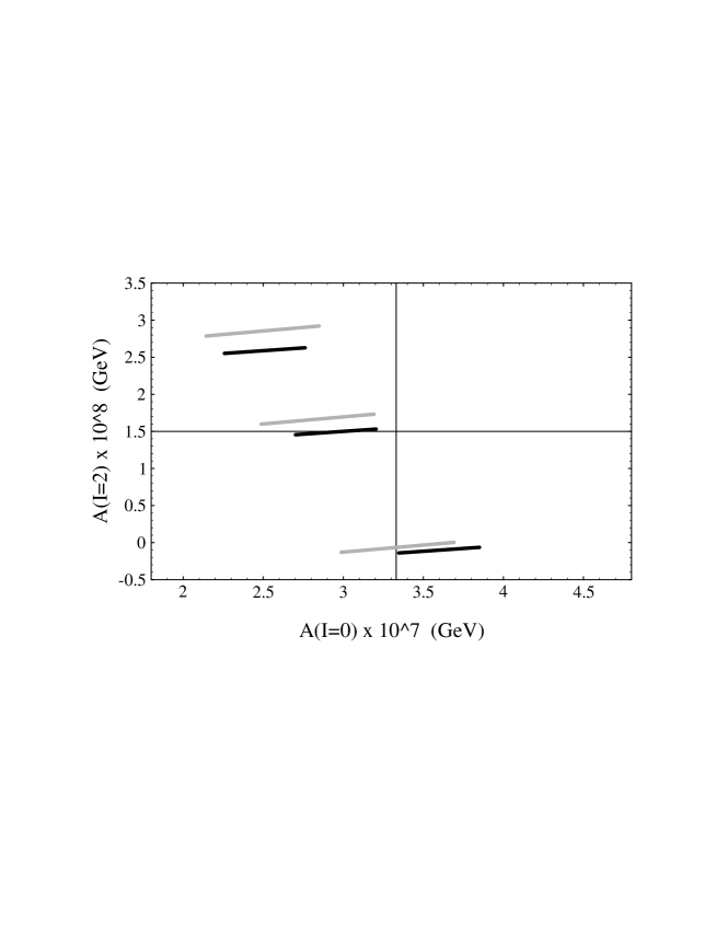
Figure 3: Same as in fig. 1 for $M=200$ MeV.

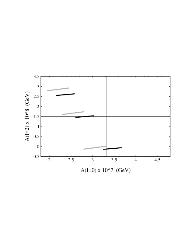
Figure 4: Same as in fig. 1 for $M=220$ MeV.

The size of $A_{2}$ is a sensitive function of the gluon condensate and the experimental value is approximately reproduced in both schemes by the central value of eq. (3.26).

Figs. 1, 2, 3 and 4 represent the main result of this paper. For any choice of $M$ in the range

$$M=160-220\quad\mbox{MeV}$$ (4.6)

the experimental values of $A_{0}$ and $A_{2}$ are reproduced by our computation by different choice of the input parameters $\left\langle\bar{q}q\right\rangle$ and $\left\langle GG\right\rangle$ that, however, remain within the ranges discussed in section 3.1. Values of $M$ smaller than 160 MeV are still consistent with the experiments, while the suppression of the gluon penguin contributions as we increase $M$ above 220 MeV would force us to quark condensate values outside the range of eq. (3.27) in order to remain close to the experimental value for $A_{0}$.

4.5 $\gamma_{5}$-scheme independence

The Wilson coefficients in eq. (2.1) depend at the NLO on the $\gamma_{5}$ scheme employed [12, 13]. In the $\chi$QM also the hadronic matrix elements depend on the $\gamma_{5}$-scheme used in the computation. The requirement that these two dependences balance each other to provide a $\gamma_{5}$-scheme independent result can be used in order to restrict the allowed values for the free parameter $M$.

The scheme dependence is not strong in the amplitudes $A_{0}$ and $A_{2}$, and, therefore, in this case, we can only restrict a range of values of $M$ for which it is reasonably under control, but nothing more. The idea is however that when examining other observables with a stronger scheme dependence as, for instance, $\varepsilon^{\prime}/\varepsilon$, we may find a substantial reduction of the scheme dependence for values of $M$ that are still within the range determined by means of $A_{0}$ and $A_{2}$. A consistent picture for the whole of kaon physics would thus emerge, with different observables concurring in a consistent determination of the free parameter $M$ as well as the range of the input parameters.

In our estimate of the hadronic matrix elements, the $\gamma_{5}$-scheme independence of $A_{0}$ turns out to be controlled by the gluonic penguins. In fact, the Wilson coefficients $z_{3-6}$ are systematically larger in the NDR scheme than in the HV scheme. On the other hand, in the NDR scheme the matrix elements of the gluonic penguins decrease with increasing $M$ faster than in the HV scheme. As a consequence, it always exists a value of $M$ for which the $\gamma_{5}$-scheme independence is achieved.

Larger values of the quark condensate gives stability for larger values of $M$. From fig. 5 and 6 one can readily see that the difference between the two schemes remains below 20% for $M$ between 140 and 240 MeV.

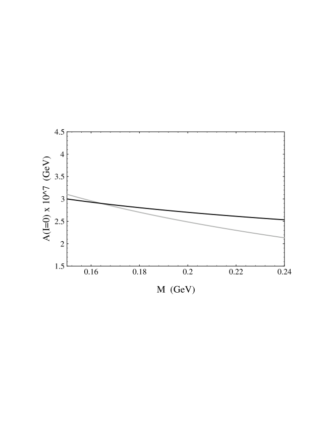
Figure 5: The $\gamma_{5}$-scheme dependence of $A_{0}$ is shown as a function of $M$. The black (grey) line represent the HV (NDR) result. We use $\left\langle\alpha_{s}GG/\pi\right\rangle=(376\ \mbox{MeV})^{4}$ and $\left\langle\bar{q}q\right\rangle=-(220\ \mbox{MeV})^{3}$. For this value of the quark condensate the stability appear near $M=160$ MeV. In the whole range of $M$ shown, the $\gamma_{5}$-scheme dependence is always below 20%.

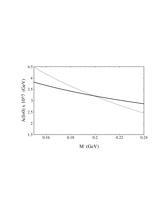
Figure 6: Same as in fig. 5 for $\left\langle\bar{q}q\right\rangle=-(280\ \mbox{MeV})^{3}$. The stability is moved at about $M=200$ MeV.

The same is not true for the amplitude $A_{2}$. In this case, the amplitude is controlled by the operators $Q_{1}$ and $Q_{2}$ only so that there is no dependence on $M$ and, accordingly, no intersection between the two schemes. The scheme dependence, however, stays well below 20%, as it can be seen in Fig. 7.

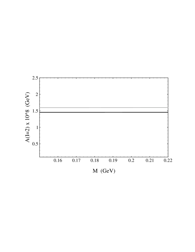
Figure 7: Same as in fig. 5 for $A_{2}$.

5 The Road to the $\Delta I=1/2$ Selection Rule

An instructive way of analyzing the relevance of the various contributions to the $\Delta I=1/2$ rule is obtained by turning on in our computation each of them as we follow the historical steps that have lead to the present understanding of the rule (fig. 8).

The point labeled by (1) in fig. 8 represents the theoretical prediction as obtained by considering the pure VSA matrix elements of $Q_{1}$ and $Q_{2}$ without the short distance renormalization of the corresponding Wilson coefficients $(\mu=m_{W})$. Point (2) represents the inclusion of the NLO renormalized Wilson coefficients, matched to the hadronic matrix elements at the scale $\mu=0.8$ GeV. This scale is large enough to make the renormalization-group analysis reliable while keeping the hadronic matrix elements in the chiral regime.

As we can see, the value for $A_{0}$ is far too small and that of $A_{2}$ too large by a factor of two.

The introduction of penguin operators (point (3)) goes in the direction of increasing $A_{0}$, but it leaves $A_{2}$ unchanged. Their effect on $A_{0}$ is not, at least in the $\chi$QM, as crucial as often claimed.

The introduction of the electroweak penguins ($Q_{7-10}$) little affects the $CP$-conserving amplitudes (point (4)), being suppressed by the smallness of their Wilson coefficients. Another isospin breaking contribution to the amplitude $A_{2}$ comes from a long-distance effect, namely the mixing between $\pi^{0}$ and $\eta$ particles. This contribution is evaluated to be

$$A_{2}^{iso-brk}\simeq-\frac{1}{3\sqrt{2}}\frac{m_{d}-m_{u}}{m_{s}}A_{0}\,.$$ (5.1)

Accordingly, we have a reduction of the amplitude $A_{2}$ represented by point (5) which compensates for the effect of the electroweak penguins. Because of the smallness of $A_{0}$ at point (5), the effect of (5.1) is very small, though it reaches the 10% level in the final point (7).

A crucial step toward the understanding of the selection rule is due to the (non-factorizable) gluon-condensate corrections (point (6)). They represent a genuine non-perturbative part of the computation. The isospin asymmetry generated by the electroweak operators is amplified in the right direction, improving dramatically $A_{2}$, that becomes close to its experimental value, while $A_{0}$ is further increased with respect to point (5). The relevance of these contributions was first pointed out in ref. [19].

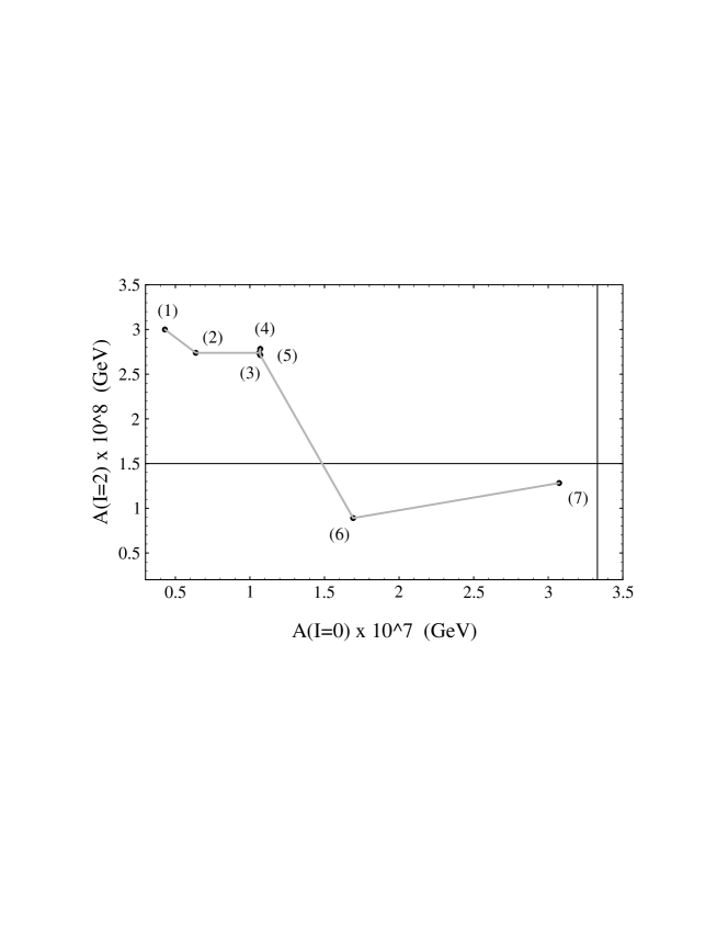
Figure 8: The road to the $\Delta I=1/2$ rule: (1) Effect of the W-induced current-current matrix elements $(Q_{1,2})$ with the neglect of short-distance QCD renormalization $(\mu=m_{W})$; (2) $\left\langle Q_{1,2}\right\rangle$ with the inclusion of the NLO Wilson coefficients at $\mu=0.8$ GeV. (3) inclusion of the gluon penguins $(Q_{3-6})$; (4) inclusion of the electro-weak penguins $(Q_{7-10})$; (5) inclusion of the $\pi^{0}-\eta$ mixing; (6) inclusion of gluon condensate corrections; (7) meson-loop renormalization. The results shown are those of the HV scheme with the central values $\left\langle\alpha_{s}GG/\pi\right\rangle=(376\>\mbox{MeV})^{4}$ and $\left\langle\bar{q}q\right\rangle=-(250\>\mbox{MeV})^{3}$, for a matching scale $\mu=0.8$ GeV and $M=180$ MeV. The experimental values are given by the cross hairs.

The meson-loop renormalization provides in our approach the final step toward the experimental results. The size of the relative renormalizations of $A_{0}$ and $A_{2}$ goes in the right direction, being large for $A_{0}$ and small for $A_{2}$. The meson loops also introduce a renormalization scale dependence in the hadronic matrix elements to be matched with that of the Wilson coefficients.

As point (7) of fig. 8 shows, the $\Delta I=1/2$ selection rule is well reproduced in the $\chi$QM, that provides not only values for the amplitudes $A_{0}$ and $A_{2}$ that are close to the experimental ones but also a satisfactory scale and $\gamma_{5}$-scheme independence of the estimate. Within 20% we also have scale independence in the matching range between 0.8 and 1 GeV.

In drawing fig. 8 we have taken the gluon and quark condensates at the central values of eqs. (3.26)–(3.27). Had we chosen, for instance, $\left\langle\alpha_{s}GG/\pi\right\rangle=(372\>\mbox{MeV})^{4}$ and $\left\langle\bar{q}q\right\rangle=-(271\>\mbox{MeV})^{3}$ we would have exactly reproduced the experimental result.

Acknowledgments

We thank our collaborator J.O. Eeg for teaching us about the $\chi$QM and for many discussions.

This work was partially supported by the EEC Human Capital and Mobility contract ERBCHRX CT 930132.

A Input Parameters

parameter	value
$V_{ud}$	0.9753
$V_{us}$	0.221
$\sin^{2}\theta_{W}$	0.2247
$m_{Z}$	91.187 GeV
$m_{W}$	80.22 GeV
$m_{b}$	4.8 GeV
$m_{c}$	1.4 GeV
$f_{\pi}=f_{\pi^{+}}$	92.4 MeV
$f_{K}=f_{K^{+}}$	113 MeV
$m_{\pi}=(m_{\pi^{+}}+m_{\pi^{0}})/2$	138 MeV
$m_{K}=m_{K^{0}}$	498 MeV
$m_{\eta}$	548 MeV
$\Lambda_{\chi}$	$2\sqrt{2}\pi f_{\pi}$
$\Lambda_{QCD}^{(4)}$	$350\pm 100$ MeV
$\overline{m}_{u}+\overline{m}_{d}$ (1 GeV)	$12\pm 2.5$ MeV
$\left\langle\bar{q}q\right\rangle$	$-(200-280\>\mbox{MeV})^{3}$
$\langle\alpha_{s}GG/\pi\rangle$	$(376\pm 47\>\mbox{MeV})^{4}$

Table 6: Table of the numerical values of the input parameters.

References

- [1] M. Gell-Mann and A. Pais, Proc. Glasgow Conf. 1954, p. 342 (Pergamon, London, 1955).
- [2] Review of Particle Properties, Phys. Rev. D 50 (1994) 1173
- [3] H.-Y. Cheng, Int. J. Mod. Phys. A 4 (1989) 495.
- [4] K.G. Wilson, Phys. Rev. 179 (1969) 1499.
- [5] M.K. Gaillard and B.W. Lee, Phys. Rev. Lett. 33 (1974) 108.
- [6] G. Altarelli and L. Maiani, Phys. Lett. B 52 (1974) 351.
- [7] M.A. Shifman, A.I. Vainshtein and V.I. Zakharov, Nucl. Phys. B 120 (1977) 316
-
[8]
Y. Dupont and T.N. Pham, Phys. Rev. D 29 (1984) 1368;
J.F. Donoghue, Phys. Rev. D 30 (1984) 1499;
M.B. Gavela et al., Phys. Lett. B 148 (1984) 225;
R.S. Chivukula, J.M. Flynn and H. Giorgi, Phys. Lett. B 171 (1986) 453. - [9] A.G. Cohen and A. Manohar, Phys. Lett. B 143 (1984) 481.
-
[10]
W.A. Bardeen A.J. Buras and J.-M. Gérard,
Phys. Lett. B 192 (1987) 138;
W.A. Bardeen, A.J. Buras and J.-M. Gerard, Nucl. Phys. B 293 (1987) 787. - [11] G. Kambor, J. Missimer and D. Wyler, Nucl. Phys. B 346 (1990) 17 and Phys. Lett. B 261 (1991) 496.
- [12] A.J. Buras, M. Jamin and M.E. Lautenbacher, Nucl. Phys. B 408 (1993) 209.
- [13] M. Ciuchini, E. Franco, G. Martinelli and L. Reina, Nucl. Phys. B 415 (1994) 403; Phys. Lett. B 301 (1993) 263.
-
[14]
L3 Coll., Phys. Lett. B 248 (1990) 464, Phys. Lett. B 257 (1991) 469;
ALEPH Coll., Phys. Lett. B 255 (1991) 623, Phys. Lett. B 257 (1991) 479;
DELPHI Coll., Z. Physik C 54 (1992) 55;
OPAL Coll., Z. Physik C 55 (1992) 1;
Mark-II Coll., Phys. Rev. Lett. 64 (1990) 987;
SLD Coll., Phys. Rev. Lett. 71 (1993) 2528. - [15] V. Antonelli, S. Bertolini, J.O. Eeg, M. Fabbrichesi and E.I. Lashin, The Weak Chiral Lagrangian as the Effective Theory of the Chiral Quark Model, preprint SISSA 43/95/EP (September 1995), hep-ph/9511255.
-
[16]
K. Nishijima, Nuovo Cim. 11 (1959) 698;
F. Gursey, Nuovo Cim. 16 (1960) 230 and Ann. Phys. (NY) 12 (1961) 91;
J.A. Cronin, Phys. Rev. 161 (1967) 1483;
S. Weinberg, Physica 96A (1979) 327;
A. Manohar and H. Georgi, Nucl. Phys. B 234 (1984) 189;
A. Manohar and G. Moore, Nucl. Phys. B 243 (1984) 55. - [17] D. Espriu, E. de Rafael and J. Taron, Nucl. Phys. B 345 (1990) 22;
-
[18]
J. Bijnens, C. Bruno and E. de Rafael, Nucl. Phys. B 390 (1993) 501;
see, also: D. Ebert, H. Reinhardt and M.K. Volkov, in Prog. Part. Nucl. Phys. vol. 33, p. 1 (Pergamon, Oxford 1994);
J. Bijnens, Phys. Rep. 265 (1996) 369. -
[19]
A. Pich and E. de Rafael, Nucl. Phys. B 358 (1991) 311;
see, also: E. De Rafael, Chiral Lagrangians and Kaon CP-violation, Lecture at TASI 1994, J.F. Donoghue, ed. (World Scientific, Singapore 1995). - [20] M. Jamin and A. Pich, Nucl. Phys. B 425 (1994) 15.
- [21] J. Heinrich et al., Phys. Lett. B 279 (1992) 140.
- [22] S. Bertolini, J.O. Eeg and M. Fabbrichesi, Nucl. Phys. B 449 (1995) 197.
-
[23]
M.A. Shifman, A.I. Vainsthain and V.I. Zakharov,
Nucl. Phys. B 120 (1977) 316;
F.J. Gilman and M.B. Wise, Phys. Rev. D 20 (1979) 2392;
J. Bijnens and M.B. Wise, Phys. Lett. B 137 (1984) 245;
M. Lusignoli, Nucl. Phys. B 325 (1989) 33. -
[24]
E. Braaten, S. Narison and A. Pich, Nucl. Phys. B 373 (1992) 581;
S. Narison, Phys. Lett. B 361 (1995) 121;
R.A. Bertlmann et al., Z. Physik C 39 (1988) 231. - [25] C.A. Dominguez and E. de Rafael, Ann. Phys. (NY) 174 (1987) 372.
-
[26]
D. Daniel et al., Phys. Rev. D 46 (1992) 3130;
D. Weingarten, Nucl. Phys. B 34 (1994) 29 (Proc. Suppl.). - [27] J. Bijnens, J. Prades and E. de Rafael, Phys. Lett. B 348 (1995) 226.
- [28] G. Buchalla, A.J. Buras and K. Harlander, Nucl. Phys. B 337 (1990) 313.
-
[29]
G.W. Kilcupp, Nucl. Phys. B 20 (1991) 417 (Proc. Suppl.);
S. Sharpe, Nucl. Phys. B 20 (1991) 429 (Proc. Suppl.);
M. Ciuchini et al., Phys. Lett. B 301 (1993) 263. - [30]