UCLA/95/TEP/37

hep-ph/9511336

November 15, 1995

Massive Loop Amplitudes from Unitarity
Z. Bern and A.G. Morgan
Department of Physics, University of California at Los Angeles,
Los Angeles, CA 90095-1547

We show, for previously uncalculated examples containing a uniform mass in the loop, that it is possible to obtain complete massive one-loop gauge theory amplitudes solely from unitarity and known ultraviolet or infrared mass singularities. In particular, we calculate four-gluon scattering via massive quark loops in QCD. The contribution of a heavy quark to five-gluon scattering with identical helicities is also presented.

1 Introduction

The computation of loop amplitudes by traditional methods is notoriously difficult involving laborious calculation. At one loop, traditional Feynman diagram techniques, augmented by computers, are in wide-spread use for up to four external particles. Beyond this, computations become significantly more complicated and traditional approaches are problematic. Non-traditional approaches have recently been used to compute all one-loop massless five-parton amplitudes [1, 2, 3] and a variety of infinite sequences of one-loop amplitudes [4, 5, 6, 7]. The technical developments which allowed for this progress include methods involving spinor helicity [8], color decompositions [9], supersymmetry [10, 11, 12], string-theory [13, 14], recursion relations [15, 5], factorization [16, 4, 17] and unitarity [18, 6, 7].

These developments have been mostly limited to massless amplitudes. However, in many physical processes, such as near particle thresholds or in the production of heavy states, one cannot neglect masses. There is, for example, some concern that the underlying cause of the apparent discrepancy between the low and high energy measurements of the strong coupling constant is due to ignoring masses [19].

In this paper we extend unitarity techniques to obtain particular examples of massive one loop amplitudes directly from tree amplitudes. Unitarity has been a useful tool in quantum field theory since its inception. The Cutkosky rules [18, 20] allow one to obtain the imaginary (absorptive) parts of one-loop amplitudes directly from tree amplitudes. Traditionally, dispersion relations are then used to reconstruct real (dispersive) parts, up to ambiguities in rational functions. Although computationally more powerful than Feynman rules, the rational function ambiguity has hampered the use of unitarity as a method for obtaining complete amplitudes.

Recently, it was shown that for certain ‘cut-constructible’ massless amplitudes – such as supersymmetric amplitudes – one may obtain the full amplitude solely from the cuts [6, 7]. This type of procedure has the inherent advantage of building loop amplitudes from tree amplitudes which are generally compact, rather than from more complicated Feynman diagrams. With this technique, massless one-loop supersymmetric amplitudes with an arbitrary number of external legs, but fixed helicity structure, have been obtained. The main new ingredient used to remove ambiguities from cut constructions is the complete knowledge of all integral functions [21, 22, 23] entering into massless one-loop amplitudes. This severely limits the analytic form of amplitudes. The cut construction method may be extended to full massless QCD by computing to higher order in the dimensional regularization parameter [24, 25]. In this way, all terms in any massless one-loop amplitude become associated with branch cuts which may be used to reconstruct the complete amplitude.

In general, one is also interested in massive theories such as QCD with heavy quarks. The amplitudes of such theories contain logarithms that depend only on masses; such functions do not have cuts in any kinematic variable. This might seem to imply that one cannot obtain all of the terms in massive amplitudes via unitarity. However, we will explicitly show for four-gluon amplitudes with a massive quark loop that the well known form of their ultraviolet or infrared-mass singularities provides sufficient information on the coefficients of all potentially ambiguous functions. We also present the result for the scattering, via a massive quark loop, of five-gluons with identical helicities. (These amplitudes have not been computed previously.) The efficiency of the method for these examples may be characterized by the fact that intermediate algebraic expressions are about the same size as final expressions for the amplitude. Due to this feature there is no need for computer assistance in performing the computations presented in this paper. This may be contrasted with Feynman diagram calculations which frequently suffer from an exponential growth in the algebra of intermediate expressions. For other five- and higher-point amplitudes, computer assistance is useful since the number of cuts and terms in the final amplitudes proliferates.

In section 2, we briefly review a few of the established techniques for computing amplitudes. Section 3 illustrates the ambiguities that are traditionally associated with unitarity based calculations. We then remove these ambiguities in section 4. In sections 5 and 6, we use the results of the previous sections to calculate all four-gluon helicity amplitudes with a heavy fermion loop. We also present the five-gluon amplitude with all identical helicities. Our conclusions are presented in section 7. We collect various useful results in the appendices.

2 Review of previous techniques

We now briefly review some of the techniques which we shall use in this paper. Two techniques that we utilize are spinor helicity and color decompositions. The reader may consult the review article of Mangano and Parke [26] for further details.

In explicit calculations with external gluons, it is usually convenient to use a spinor helicity basis [8] which rewrites all polarization vectors in terms of massless Weyl spinors $|k^{\pm}\rangle$. In the formulation of Xu, Zhang and Chang the plus and minus helicity polarization vectors are expressed as

$$\varepsilon^{+}_{\mu}(k;q)={\left\langle\smash{q}{\vphantom{1}}^{-}\right|{\gamma_{\mu}}\left|\smash{k}{\vphantom{1}}^{-}\right\rangle\over\sqrt{2}\left\langle q\,k\right\rangle}\,,\hskip 28.45274pt\varepsilon^{-}_{\mu}(k;q)={\left\langle\smash{q}{\vphantom{1}}^{+}\right|{\gamma_{\mu}}\left|\smash{k}{\vphantom{1}}^{+}\right\rangle\over\sqrt{2}\left[k\,q\right]}\,,$$

where $q$ is an arbitrary null ‘reference momentum’ which drops out of the final gauge-invariant amplitudes. The cuts of amplitudes are also gauge invariant, so one may evaluate different cuts using independent choices of reference momenta. We use the convenient notation

$$\langle k_{i}^{-}|k_{j}^{+}\rangle\equiv\langle ij\rangle\,,\hskip 56.9055pt\langle k_{i}^{+}|k_{j}^{-}\rangle\equiv[ij]\,.$$

These spinor products are anti-symmetric and satisfy

$$\left\langle i\,j\right\rangle\left[j\,i\right]=2k_{i}\cdot k_{j}\,.$$

This provides for an extremely compact representation of gluon amplitudes. A useful identity is

$$\left\langle\smash{a}{\vphantom{1}}\right|{{\raise-0.34723pt\hbox to4.66318pt{\hss/\hss}\hbox to0.0pt{\hss$\varepsilon$}}^{\pm}(k;q)}\left|\smash{b}{\vphantom{1}}\right\rangle=\pm\frac{\sqrt{2}}{\langle q^{\mp}|\ k^{\pm}\rangle}\langle a|\left[|q^{\pm}\rangle\langle k^{\pm}|+|k^{\mp}\rangle\langle q^{\mp}|\right]|b\rangle\,,$$

where either $\langle a|$ or $|b\rangle$ are spinors with four-dimensional momenta.

For loop amplitudes, to maximize the benefit of the spinor helicity method we must choose an appropriate regularization scheme. In conventional dimensional regularization [27], the polarization vectors are taken to be $(4-2\epsilon)$-dimensional; this is incompatible with spinor helicity which assumes that the polarization vectors are four dimensional. An alternative is to modify the regularization scheme to define the polarization vectors to be four dimensional. One also defines all internal and external states to be four-dimensional and only continues loop momentum and phase-space integrals to $(4-2\epsilon)$ dimensions. This is the four-dimensional-helicity (FDH) scheme [13], which has been shown to be equivalent [12] to an appropriate helicity formulation of Siegel’s dimensional-reduction scheme [28] at one-loop. Dimensional regularization rules, which may be used in cut calculations of fermion loops, are reviewed in appendix C. The conversion between schemes has been given in ref. [12], so one may choose whichever scheme is simplest to perform calculations in. In this paper we work exclusively in the FDH scheme but for fermion or scalar loops this gives the same results as in the ’t Hooft-Veltman [29, 27] scheme.

$SU(N_{c})$ gauge theory amplitudes can be written in terms of independent color-ordered partial amplitudes multiplied by an associated color trace [9, 26]. One of the key features of the partial amplitudes is that the external legs have a fixed ordering. For the one-loop four-gluon amplitude with a fundamental representation loop the decomposition is

 

$${{\cal A}_{4}^{\rm 1-loop}=g^{4}\mu_{R}^{2\epsilon}\sum_{\sigma}}$$

 

where the sum over $\sigma$ includes all non-cyclic permutations of the indices $\sigma(n)$ and the $T^{a}$ are fundamental representation color matrices (normalized so that ${\rm tr}(T^{a}T^{b})=\delta^{ab}$). We have explicitly extracted the coupling and a factor of $\mu_{R}^{2\epsilon}$ from $A_{n}$, where $\mu_{R}$ is the renormalization scale. (We have abbreviated the dependence of $A_{4}$ on the outgoing momenta $k_{j}$ and helicities $\lambda_{j}$ by writing the label $j$ alone.) For adjoint representation loops there is an analogous decomposition with up to two color traces in each term. A similar decomposition in terms of ‘primitive amplitudes’ can also be performed for the case where some of the external particles are in the fundamental representation [3]. (In refs. [1, 3], for example, it was slightly more convenient to extract an overall factor of $N_{c}$ from the color ordered amplitudes, $A_{n}$, but since we only deal with fundamental representation loops in this paper there is no need for this.)

An essential feature of this decomposition is that the partial amplitudes, $A_{n}$, are described by diagrams with a fixed cyclic ordering of external legs. In this paper we deal exclusively with such amplitudes.

3 Naive application of Cutkosky rules

In this section we demonstrate how a naive application of the Cutkosky rules can miss contributions to a complete one-loop amplitude. Traditionally, one first computes the imaginary (absorptive) part of an amplitude by evaluating a four-dimensional phase-space integral. (The phase-space integrals are not ultraviolet divergent and therefore converge in four-dimensions.) The real (dispersive) part is then reconstructed via a dispersion relation. We perform the cut calculation a bit differently; since we want the complete amplitude, it is convenient to replace the phase-space integral with an unrestricted loop momentum integral which has the correct branch cuts [6, 7]. This allows us to simultaneously construct the real and imaginary parts. The ambiguities that we encounter are equivalent to those of the more conventional approach.

We will compute cuts of massive amplitudes in all possible channels in an attempt to reconstruct their functional form. We consider the amplitude, not in a physical kinematic configuration, but in a region where exactly one of the momentum invariants is taken to be above threshold, and the rest are negative (space-like). In this way we isolate cuts in a single momentum channel. Furthermore, following refs. [6, 7], we apply the Cutkosky rules at the amplitude level, rather than at the diagram level. This is advantageous because amplitudes are generally much more compact than diagrams.

Consider the $s$-channel ($s=(k_{1}+k_{2})^{2}$) cut of the four-gluon amplitude pictorially represented in fig. 1a, and given by the phase-space integral

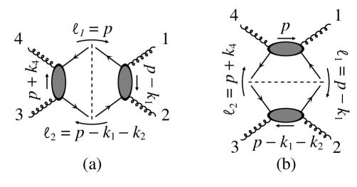
Figure 1: The $s$- and $t$-channel cuts of a one-loop four-gluon amplitude. The cut lines represent either a fermion or scalar.

 

$${-i\,{\rm Disc}\;A_{4}(1,2,3,4)\Bigr{|}_{s\rm-cut}}$$

 

where $\ell_{1}=p$ and $\ell_{2}=p-k_{1}-k_{2}$, $m$ is the mass of the particle in the loop, $\delta^{\tiny(+)}$ is the positive energy branch of the delta-function and ‘Disc’ means the discontinuity across the branch cut. Note that, in performing the sewing of the tree amplitudes, we have maintained the clockwise ordering of the legs, as required by the color decomposition.

Since we wish to reconstruct the full amplitude and not just the imaginary (or absorptive) part, it is convenient to replace the phase-space integral with the cut of an unrestricted loop momentum integral [6]. This is accomplished by replacing the $\delta$-functions, which impose on-shellness, with propagators: we replace eq. ($(3.1)$) with

$$\,\vbox{\openup 3.0pt\halign{\strut\hfil$\displaystyle{#}$&$ \displaystyle{{}#}$\hfil\cr A_{4}(1,2,3,4)\Bigr{|}_{s\rm-cut}&=\int{d^{4}p\over(2\pi)^{4}}\;{i\over\ell_{1}^{2}-m^{2}}\,A^{\rm tree}_{4}(-\ell_{1},1,2,\ell_{2})\,{i\over\ell_{2}^{2}-m^{2}}\,A^{\rm tree}_{4}(-\ell_{2},3,4,\ell_{1})\cr}}\,\Bigr{|}_{s\rm-cut}\,.$$

As indicated this equation is valid only on the $s$-cut. A similar equation holds on the $t$-cut (where $t=(k_{2}+k_{3})^{2}$), depicted in fig. 1b. Up to potential ambiguities in rational functions, one obtains the full amplitude by combining the two cuts into a single function.

For example, consider the amplitude $A_{4}(1^{+},2^{+},3^{+},4^{+})$ with a massive scalar in the loop. This amplitude is useful for illustrative purposes because it is particularly simple. The tree amplitudes entering the two sides are easily computed from Feynman diagrams and are given by

 

$${A_{4}^{\rm tree}(-\ell_{1},1^{+},2^{+},\ell_{2})}$$

 

where legs $\ell_{1}$ and $\ell_{2}$ represent the cut scalar lines. From eq. ($(3.2)$) the scalar loop contribution to the four-gluon amplitude is

 

$${A_{4}}$$

 

where $I_{4}^{D=4}$ is the scalar integral box function given in eq. ($(\mathrm{A}.6)$) of appendix A. The function $I_{4}^{D=4}$ contains branch cuts since it contains logarithms and dilogarithms. At this stage the equality of both sides of the equation is only for the cut in the $s$-channel.

The $t$-channel cut is similar and may be obtained by relabeling the legs by $1\leftrightarrow 3$. Using the identity

$${\left[2\,3\right]\left[4\,1\right]\over\left\langle 2\,3\right\rangle\left\langle 4\,1\right\rangle}={\left[1\,2\right]\left[3\,4\right]\over\left\langle 1\,2\right\rangle\left\langle 3\,4\right\rangle}\,,$$

the full amplitude is found to have the form

$$A_{4}(1^{+},2^{+},3^{+},4^{+})={im^{4}\over 16\pi^{2}}{\left[1\,2\right]\left[3\,4\right]\over\left\langle 1\,2\right\rangle\left\langle 3\,4\right\rangle}I_{4}^{D=4}+\hbox{rational}\,,$$

since it has the correct branch cuts. The rational terms have no cuts. Indeed, if we compare this to the correct result for the amplitude

$$\,\vbox{\openup 3.0pt\halign{\strut\hfil$\displaystyle{#}$&$ \displaystyle{{}#}$\hfil\cr A_{4}(1^{+},2^{+},3^{+},4^{+})&={i\over 16\pi^{2}}{\left[1\,2\right]\left[3\,4\right]\over\left\langle 1\,2\right\rangle\left\langle 3\,4\right\rangle}\Bigl{(}m^{4}I_{4}^{D=4}-{1\over 6}\Bigr{)}\crcr}}\,\,,$$

we explicitly see that the last term was missed by our naive application of the Cutkosky rules. We note that setting $m=0$ in eq. ($(3.7)$) gives the correct massless scalar loop result [13].

4 Fixing the ambiguity

We now demonstrate that the last term in eq. ($(3.7)$), which is cut-free, may be obtained from the first one with little additional work but with a more careful application of unitarity.

4.1 Cuts with dimensional regularization

The Cutkosky rules are valid in arbitrary dimensions—that is they may be used with dimensional regularization. By working to all orders in the dimensional regularization parameter, $\epsilon=(4-D)/2$, the number of potential ambiguities is greatly reduced. In a massless theory, it is clear that there are no polynomial ambiguities in dimensionally regularized expressions. All terms necessarily must contain cuts since the dimensions are shifted by $-2\epsilon$ and must therefore be proportional to factors of the form $(-K^{2})^{-\epsilon}$, where $K^{2}$ is some kinematic variable. For example, in the massless case, by working to higher order in $\epsilon$, the $1/6$ in eq. ($(3.7)$) appears as

$$-{(-s)^{1-\epsilon}+(-t)^{1-\epsilon}\over 6(s+t)}+\cdots={1\over 6}+{\cal O}(\epsilon)\,,$$

which contains cuts at ${\cal O}(\epsilon)$ linked to the $1/6$. Indeed, this observation may be used to compute the rational part of massless amplitudes directly from the cuts [24, 25].

For massive theories this simple argument requires modification, because of the presence of additional dimensionful parameters (the masses). A factor of $m^{-2\epsilon}$ can in principle soak up dimensions to generate terms without cuts. We will return to this issue at the end of this section.

As a first step in removing the rational function ambiguities, we modify the calculation of the previous section to be valid to all orders in the dimensional regularization parameter, $\epsilon$; as we shall see this automatically removes most ambiguities. We consider again the cut integral in eq. ($(3.4)$) and fig. 1a, except this time we replace the four-dimensional loop momenta, $\ell_{1}$ and $\ell_{2}$, with $(4-2\epsilon)$-dimensional ones. A simple way to implement this is to modify the on-shell condition on the cuts to $\ell_{1}^{2}-\mu^{2}=m^{2}$ and $\ell_{2}^{2}-\mu^{2}=m^{2}$, where $\ell_{1}$ and $\ell_{2}$ are left in four-dimensions, but $\mu^{\alpha}$ is a vector representing the $(-2\epsilon)$-dimensional part of the loop momentum. (See Appendices A.2 and C.) With this notation, it is easy to see that the dimensionally regularized forms of the tree amplitudes are obtained from eq. ($(3.4)$) by shifting $m^{2}\rightarrow m^{2}+\mu^{2}$.

Thus, the dimensionally regularized expression for the $s$-channel cut replacing eq. ($(3.4)$) is

 

$${A_{4}^{\rm scalar}(1^{+},2^{+},3^{+},4^{+})\Bigr{|}_{s\rm-cut}}$$

 

where we have explicitly separated out the integration over the $(-2\epsilon)$-dimensions. The box denominator is

$${\cal D}_{4}\equiv(p^{2}-\mu^{2}-m^{2})((p-k_{1})^{2}-\mu^{2}-m^{2})((p-k_{1}-k_{2})^{2}-\mu^{2}-m^{2})((p+k_{4})^{2}-\mu^{2}-m^{2})\,.$$

In obtaining this form we used the standard prescription that a four-dimensional vector is orthogonal to a $(-2\epsilon)$-dimensional one. This representation of dimensional regularization follows the one used in its original derivation [29] and has recently been used by Mahlon in his recursive approach [5].

As discussed in appendix A.2, integrals with powers of $\mu$ in the numerator may be expressed in terms of higher dimension loop integrals,

 

$${{}I_{n}[(\mu^{2})^{r}]\equiv i(-1)^{n+1}(4\pi)^{2-\epsilon}\int{d^{4}p\over(2\pi)^{4}}{d^{-2\epsilon}\mu\over(2\pi)^{-2\epsilon}}\,{(\mu^{2})^{r}\over{\cal D}_{n}}=-\epsilon(1-\epsilon)(2-\epsilon)\cdots(r-1-\epsilon)\,I_{n}^{D=2r+4-2\epsilon}\,,}$$

 

where $I_{n}^{D=2r+4-2\epsilon}$ is the scalar loop $n$-point integral function evaluated in ($2r+4-2\epsilon$)-dimensions and ${\cal D}_{n}$ is the appropriate product of denominators. Thus, the correct $s$-channel cut to all orders in $\epsilon$ is

 

$${A_{4}^{\rm scalar}(1^{+},2^{+},3^{+},4^{+})\Bigr{|}_{s\rm-cut}}$$

 

where (see appendix A.4)

$$K_{4}\equiv I_{4}[(m^{2}+\mu^{2})^{2}]=m^{4}I_{4}^{D=4-2\epsilon}-2m^{2}\epsilon\,I_{4}^{D=6-2\epsilon}-\epsilon(1-\epsilon)\,I_{4}^{D=8-2\epsilon}\;.$$

Once again the $t$-channel cut may be obtained by relabeling $k_{1}\leftrightarrow k_{3}$, so that the function

$$A_{4}^{\rm scalar}(1^{+},2^{+},3^{+},4^{+})={i\over(4\pi)^{2-\epsilon}}{\left[1\,2\right]\left[3\,4\right]\over\left\langle 1\,2\right\rangle\left\langle 3\,4\right\rangle}\,K_{4}+f(m^{2})\,,$$

has the correct cuts in both the $s$ and $t$ channels. The function $f(m^{2})$ has no branch cuts in any kinematic channel; it has a form $\sim\!m^{-2\epsilon}$, but may contain rational functions of kinematics variables.

4.2 Fixing the remaining ambiguity

In appendix B we show that, for the four-gluon amplitudes considered in this paper, the following procedure uniquely fixes all cut-free functions.

1. Add in the tadpole function $I_{1}$ with a coefficient adjusted so that the quadratic ultraviolet divergence vanishes. (The quadratic divergences cancel in gluon amplitudes as discussed, for example, in ref. [20].) This may be implemented by dropping all explicit $I_{1}$ functions, then substituting $J_{2}\rightarrow J_{2}+I_{1}$ and $I_{2}^{D=6-2\epsilon}\rightarrow I_{2}^{D=6-2\epsilon}-I_{1}$. These integral functions are defined in eqs. ($(\mathrm{A}.2)$), ($(\mathrm{A}.12)$) and ($(\mathrm{A}.26)$).

2. Add in the bubble function $I_{2}(0)$ with a coefficient adjusted so that the ultraviolet divergence of the amplitude agrees with the well known one. The ultraviolet divergences are

   $$A_{n}^{\rm loop}\Bigr{|}_{\rm UV\ singular}={1\over(4\pi)^{2-\epsilon}}{\Gamma(1+\epsilon)\over\epsilon}(n-2)\Bigl{(}{11N_{c}\over 6}-{n_{\!f}\over 3}-{n_{s}\over 12}\Bigr{)}\,A^{\rm tree}_{n}\,,$$

   for a theory with $N_{c}$ colors, $n_{\!f}$ fermion flavors and $n_{s}$ complex scalars. The first contribution in the parenthesis is from a gluon loop and the remaining two from fermion and scalar loops.

We will use these rules for fixing all cut-free functions in the amplitudes presented in this paper.

As an alternative to the second step, we may use the known infrared behavior as the masses vanish. For massless QCD, the dimensionally regularized infrared divergences have been categorized in refs. [30]. This may be used to fix the coefficients of all $\ln(m_{i})$ terms as $m_{i}\rightarrow 0$. In this limit the matching condition for infrared singularities is

$$\ln(m_{i}^{2})\rightarrow{1\over\epsilon}+\cdots$$

In general, the infrared properties are more powerful since we can use them to fix coefficients when there are multiple masses present in an amplitude.

For the amplitudes considered here, we find that the second step is equivalent to adding in the cut-free self-energy diagrams on external legs. For each external gluon leg the bubble contribution is $A^{\rm tree}\,{\cal F}/2$, where

$${{\cal F}}_{\rm scalar}=-{1\over(4\pi)^{2-\epsilon}}{\Gamma(1+\epsilon)\over 6\epsilon}\,m^{-2\epsilon}=-{1\over 6}\,{1\over(4\pi)^{2-\epsilon}}\,I_{2}(0)\,,$$

and

$${{\cal F}}_{\rm fermion}=-{1\over(4\pi)^{2-\epsilon}}{2\Gamma(1+\epsilon)\over 3\epsilon}\,m^{-2\epsilon}=-{2\over 3}\,{1\over(4\pi)^{2-\epsilon}}\,I_{2}(0)\,,$$

corresponding to scalar and fermion loop contributions.

For the $A_{4}^{\rm scalar}(1^{+},2^{+},3^{+},4^{+})$, the two steps are trivial because $A^{\rm tree}$ vanishes and there are no ultraviolet divergences. This means that $f(m^{2})=0$ in eq. ($(4.7)$) so that

$$A_{4}^{\rm scalar}(1^{+},2^{+},3^{+},4^{+})={i\over(4\pi)^{2-\epsilon}}{\left[1\,2\right]\left[3\,4\right]\over\left\langle 1\,2\right\rangle\left\langle 3\,4\right\rangle}K_{4}$$

is the complete amplitude valid to all orders in $\epsilon$.

The last two terms in $K_{4}$, defined in eq. ($(4.6)$), are proportional to $\epsilon$ and will contribute through ${\cal O}(\epsilon^{0})$ only if the integrals contain an $\epsilon^{-1}$. The integral $I_{4}^{D=6-2\epsilon}$ is finite, but $I_{4}^{D=8-2\epsilon}$ has an ultraviolet divergence. Extracting this divergence either by direct loop integration, or by use of the integral recursion relation ($(\mathrm{A}.12)$), we have

$$-\epsilon(1-\epsilon)I_{4}^{D=8-2\epsilon}=-{1\over 6}+{\cal O}(\epsilon)\,,$$

which gives the missing rational term in eq. ($(3.6)$). Hence, eq. ($(4.12)$) agrees with the correct result ($(3.7)$) and contains all rational functions through ${\cal O}(\epsilon^{0})$. Since the ultraviolet divergences of the integral functions are independent of masses, this rational contribution is identical to the contribution in the massless case, through ${\cal O}(\epsilon^{0})$. This feature holds for all the amplitudes presented in this paper.

5 Fermion loop amplitudes

In this section we consider fermion loop amplitudes. Fermions are slightly more complicated than scalars as one must deal with Dirac algebra, a summary of which is presented in appendix C. Apart from this, the techniques used in the previous section for the scalar loop carry over to fermion calculations.

5.1 The $A_{4}(1^{+},2^{+},3^{+},4^{+})$ amplitude

As a first example, we reconsider the all plus helicity amplitude but with a massive fermion loop instead of a massive scalar loop. In this case the tree amplitudes appearing on both sides of the $s$-channel cut (see fig. 1a) are

 

$${A_{4}^{\rm tree}(-L_{1}^{f},1^{+},2^{+},L_{2}^{f})}$$

 

where $\omega_{\pm}={1\over 2}(1\pm\gamma_{5})$, capitalized momenta are $(4-2\epsilon)$-dimensional and lower case momenta are four-dimensional. (See appendix A.) In these tree amplitudes we suppress the distinction between fermion and anti-fermion spinors: $u(p)$ versus $v(p)$. We find this convenient since it provides a uniform notation for both types of spinors. When the momentum follows the direction of the fermion arrow it represents a fermion state. Conversely, when the momentum flows against the arrow we have an anti-fermion state. However, using this convention an overall sign error is made for the contribution of a $v\bar{v}$ pair; $\sum u(-p)\bar{u}(-p)=-{\raise-1.31944pt\hbox to5.03125pt{\hss/\hss}\hbox to0.0pt{\hss$p$}}+m=-\sum v(p)\bar{v}(p)$. Since this is an overall sign, we may easily correct for it by hand. Alternatively, one may work with both $u$ and $v$ to obtain identical results.

The method for obtaining the cuts is identical to that of the scalar case in eq. ($(4.2)$), except that instead of $(\mu^{2}+m^{2})^{2}$ the numerator is initially

 

$${-\langle-\!L_{1}|\omega_{+}({\raise-1.31944pt\hbox to6.02548pt{\hss/\hss}\hbox to0.0pt{\hss$\mu$}}+m)}$$

 

where the explicit overall minus sign compensates for our suppression of the distinction between fermions and anti-fermions. Since /$\mu$ (like $m$) commutes freely (see eq. ($(\mathrm{C}.7)$)) with the helicity projection operator, $\omega_{+}$, we find that the ${\raise 0.97221pt\hbox to4.16669pt{\hss/\hss}\hbox to0.0pt{\hss$\ell$}}_{i}$ in the above trace cancel. For example the term,

$$\cdots\omega_{+}\,({\raise-1.31944pt\hbox to6.02548pt{\hss/\hss}\hbox to0.0pt{\hss$\mu$}}+m){\raise 0.97221pt\hbox to4.16669pt{\hss/\hss}\hbox to0.0pt{\hss$\ell$}}_{1}\,\omega_{+}\,\cdots=\cdots({\raise-1.31944pt\hbox to6.02548pt{\hss/\hss}\hbox to0.0pt{\hss$\mu$}}+m)\,\omega_{+}\,{\raise 0.97221pt\hbox to4.16669pt{\hss/\hss}\hbox to0.0pt{\hss$\ell$}}_{1}\,\omega_{+}\,\cdots=0\,.$$

The trace thus reduces to a combination of /$\mu$ and $m$ containing terms. We readily evaluate what remains as,

$${\rm tr}[({\raise-1.31944pt\hbox to6.02548pt{\hss/\hss}\hbox to0.0pt{\hss$\mu$}}-m)\omega_{+}({\raise-1.31944pt\hbox to6.02548pt{\hss/\hss}\hbox to0.0pt{\hss$\mu$}}+m)({\raise-1.31944pt\hbox to6.02548pt{\hss/\hss}\hbox to0.0pt{\hss$\mu$}}-m)\omega_{+}({\raise-1.31944pt\hbox to6.02548pt{\hss/\hss}\hbox to0.0pt{\hss$\mu$}}+m)]={\rm tr}[\omega_{+}({\raise-1.31944pt\hbox to6.02548pt{\hss/\hss}\hbox to0.0pt{\hss$\mu$}}^{2}-m^{2})^{2}]=2(\mu^{2}+m^{2})^{2}\,,$$

so that

$$A_{4}^{{\rm fermion}}(1^{+},2^{+},3^{+},4^{+})=-{2i\over(4\pi)^{2-\epsilon}}{\left[1\,2\right]\left[3\,4\right]\over\left\langle 1\,2\right\rangle\left\langle 3\,4\right\rangle}K_{4}\,,$$

where $K_{4}$ is defined in eq. ($(4.6)$). We have fixed the cut-free function, by following the same steps as for the scalar loop case ($(4.12)$). Thus for this helicity, the contribution for a Dirac fermion is minus twice that of a complex scalar given in eq. ($(4.12)$). This is the correct result as may be verified from a supersymmetry identity [10]. In summary, for this helicity, we have obtained the correct result for a massive quark loop, with little more work than with a naive application of unitarity.

5.2 The $A_{4}(1^{-},2^{-},3^{+},4^{+})$ amplitude

Having calculated the simplest of the closed fermion loop sub-amplitudes consider now one of the more difficult ones. The $A_{4}(1^{-},2^{-},3^{+},4^{+})$ sub-amplitude does not have an $s\leftrightarrow t$ exchange symmetry. Accordingly, we must explicitly calculate both cuts and combine the information to obtain the complete result. Also, this amplitude contains non-vanishing cut-free functions whose coefficients will be fixed from the ultraviolet divergences.

The easier cut is in the $s$-channel, so we calculate it first. The required tree-level amplitudes are,

 

$${A_{4}^{\rm tree}(-L_{1}^{f},1^{-},2^{-},L_{2}^{f})}$$

 

As before, these combine to give a contribution to the $s$-cut,

 

$${A_{4}(1^{-},2^{-},3^{+},4^{+})\Bigr{|}_{s\rm-cut}}$$

 

where $\ell_{1}=p$, $\ell_{2}=p-k_{1}-k_{2}$ and we use (see ref. [26])

$${\left\langle 1\,2\right\rangle\left[3\,4\right]\over\left[1\,2\right]\left\langle 3\,4\right\rangle}=-{t\over s}\,{\left\langle 1\,2\right\rangle^{4}\over\left\langle 1\,2\right\rangle\left\langle 2\,3\right\rangle\left\langle 3\,4\right\rangle\left\langle 4\,1\right\rangle}=i\,{t\over s}\,A_{4}^{\rm tree}(1^{-},2^{-},3^{+},4^{+})\,.$$

Concentrating on the numerator Dirac algebra under the integral, we create a trace,

 

$${\langle-\!L_{1}|\omega_{-}({\raise-1.31944pt\hbox to6.02548pt{\hss/\hss}\hbox to0.0pt{\hss$\mu$}}+m)|-\!L_{2}\rangle}$$

 

Unlike the all plus case, the helicity projection operators do not cancel the four-dimensional momenta. Instead they cancel the $({\raise-1.31944pt\hbox to6.02548pt{\hss/\hss}\hbox to0.0pt{\hss$\mu$}}-m)$ contributions from the spinors on the cut. The above trace reduces to,

 

$${{\rm tr}[\omega_{+}{\raise 0.97221pt\hbox to4.16669pt{\hss/\hss}\hbox to0.0pt{\hss$\ell$}}_{1}({\raise-1.31944pt\hbox to6.02548pt{\hss/\hss}\hbox to0.0pt{\hss$\mu$}}+m){\raise 0.97221pt\hbox to4.16669pt{\hss/\hss}\hbox to0.0pt{\hss$\ell$}}_{2}({\raise-1.31944pt\hbox to6.02548pt{\hss/\hss}\hbox to0.0pt{\hss$\mu$}}+m)]}$$

 

where we have used the fact that on the cut $\ell_{1}^{2}=\ell_{2}^{2}=\mu^{2}+m^{2}$. This integrand exhibits a supersymmetry decomposition as the first term is identical (up to an overall factor of $-2$) to the contribution of complex scalar loop.

Performing the integration, the $s$-cut of the amplitude becomes

$$A_{4}^{{\rm fermion}}(1^{-},2^{-},3^{+},4^{+})\Bigr{|}_{s\rm-cut}=-{1\over(4\pi)^{2-\epsilon}}A_{4}^{\rm tree}\Bigl{(}-2{t\over s}\,K_{4}+t\,J_{4}\Bigr{)}\Bigr{|}_{s\rm-cut}\,,$$

where $J_{4}$ and $K_{4}$ are defined in eqs. ($(\mathrm{A}.24)$) and ($(\mathrm{A}.25)$).

The $t$-cut, depicted in fig. 1b, is more complicated. It may be constructed from the following two tree amplitudes,

 

$${A_{4}^{\rm tree}(-L_{1}^{f},2^{-},3^{+},L_{2}^{f})}$$

 

where the reference momenta $q_{i}$ for the polarization vectors $\varepsilon_{i}$ are are $q_{2}=k_{3}$, $q_{3}=k_{2}$, $q_{4}=k_{1}$, and $q_{1}=k_{4}$. This is a particularly good choice of reference momenta as each tree amplitude is described by a single Feynman diagram. As depicted in fig. 1b, for the $t$-channel the cut momenta are

$$\ell_{1}=p-k_{1}\,,\hskip 56.9055pt\ell_{2}=p+k_{4}\,.$$

This representation of the tree amplitudes may be directly obtained from Feynman diagrams after using the spinor helicity form of the polarization vectors. (As discussed in appendix C, identity ($(2.4)$) may be used on the /$\varepsilon$ only when it is adjacent to a four-dimensional quantity.)

Using eq. ($(3.1)$) and combining the two tree amplitudes into a trace, the $t$-cut becomes,

 

$${A_{4}^{\rm fermion}(1^{-},2^{-},3^{+},4^{+})\Bigr{|}_{t\rm-cut}}$$

 

The numerator may be rewritten as

 

$${{\cal N}}$$

 

where

 

$${{\cal N}_{1}}$$

 

We have dropped terms with an odd power of $\mu^{\alpha}$ (see appendix A for the relevant discussion). ${\cal N}_{1}$ may be recognized as the numerator of a cut complex scalar loop, while the second is the additional piece for a fermion loop. Thus, this integrand again obeys a supersymmetry decomposition.

To evaluate the amplitudes, we use spinor helicity. From eq. ($(2.1)$), and the choice of reference momenta given below eq. ($(5.12)$), the polarization vectors satisfy

 

$${{}\varepsilon_{1}^{-}\,\cdot\,\varepsilon_{3}^{+}={\left\langle 1\,2\right\rangle\left[3\,4\right]\over\left\langle 2\,3\right\rangle\left[1\,4\right]}\,,\hskip 28.45274pt\varepsilon_{1}^{-}\,\cdot\,\ell_{2}={\left\langle\smash{4}{\vphantom{1}}^{+}\right|{{\raise 0.97221pt\hbox to4.16669pt{\hss/\hss}\hbox to0.0pt{\hss$\ell$}}_{1}}\left|\smash{1}{\vphantom{1}}^{+}\right\rangle\over\sqrt{2}\left[1\,4\right]}\,,\hskip 28.45274pt\varepsilon_{2}^{-}\,\cdot\,\ell_{1}={\left\langle\smash{3}{\vphantom{1}}^{+}\right|{{\raise 0.97221pt\hbox to4.16669pt{\hss/\hss}\hbox to0.0pt{\hss$\ell$}}_{1}}\left|\smash{2}{\vphantom{1}}^{+}\right\rangle\over\sqrt{2}\left[2\,3\right]}\,,}$$

 

It is convenient to evaluate separately the two numerator terms of eq. ($(5.15)$). The first corresponds, up to a factor of $-2$, to the contribution of a complex scalar loop, whose numerator is

 

$${{\cal N}_{1}}$$

 

By multiplying and dividing by $\left\langle 3\,4\right\rangle^{2}\left[1\,2\right]^{2}$, ${\cal N}_{1}$ can be rewritten in terms of a trace as

$${{\cal N}_{1}={1\over t^{2}}{\left\langle\smash{2}{\vphantom{1}}^{-}\right|{{\raise 0.97221pt\hbox to4.16669pt{\hss/\hss}\hbox to0.0pt{\hss$\ell$}}_{1}}\left|\smash{3}{\vphantom{1}}^{-}\right\rangle}^{2}{\left\langle 3\,4\right\rangle^{2}\over\left\langle 3\,4\right\rangle^{2}}{\left\langle\smash{4}{\vphantom{1}}^{+}\right|{{\raise 0.97221pt\hbox to4.16669pt{\hss/\hss}\hbox to0.0pt{\hss$\ell$}}_{1}}\left|\smash{1}{\vphantom{1}}^{+}\right\rangle}^{2}{\left[1\,2\right]^{2}\over\left[1\,2\right]^{2}}={i\over s^{3}t}\,A_{4}^{\rm tree}(1^{-},2^{-},3^{+},4^{+}){\rm tr}_{+}[\ell 34\ell 12\ell 34\ell 12]}\,,$$

where we have defined $\ell_{1}\equiv\ell$, and for brevity represent the external momenta by their indices and neglect slashing the momenta inside the trace. (We use the notation, ${\rm tr}_{\pm}(\ldots)={\rm tr}(\omega_{\pm}\ldots)$.) Since tensor box integrals are generally difficult to evaluate (without the aid of a computer), we will avoid such terms. To simplify the trace, we commute the $\ell$s within the trace towards each other. This generates more simple integrals, with inverse propagators or fewer powers of loop momentum in the numerator:

 

$${{\rm tr}_{+}[\ell 34\ell 12\ell 34\ell 12]}$$

 

Using

$$\left(\ell\,1\right)\equiv 2\,\ell\cdot k_{1}=p^{2}-\mu^{2}-m^{2}\,,\hskip 42.67912pt\left(\ell\,2\right)\equiv 2\,\ell\cdot k_{2}=-(p-k_{1}-k_{2})^{2}+\mu^{2}+m^{2}\,,$$

this becomes

 

$${{}{\rm tr}_{+}[\ell 34\ell 12\ell 342](p^{2}-\mu^{2}-m^{2})+{\rm tr}_{+}[\ell 34\ell 12\ell 341]((p-k_{1}-k_{2})^{2}-\mu^{2}-m^{2})}$$

 

which exhibits inverse propagators in the numerator. After cancelling these inverse propagators, against those present in eq. ($(5.14)$), we obtain tensor triangle and scalar box integrals.

One way to evaluate the tensor integrals is via Feynman parameterization. A convenient way to do this is to have a uniform labeling of Feynman parameters for all diagrams: for the triangles, the Feynman parameter corresponding to the missing internal propagator is set to zero. With this convention, the Feynman parameter shift for all diagrams is,

$$\ell=p-k_{1}=q-k_{1}a_{1}+k_{2}(a_{3}+a_{4})+k_{3}a_{4}\,,$$

where $q$ is the shifted loop momentum. For example, the first term in eq. ($(5.22)$) corresponds to the triangle integral

$${i\over s^{3}t}\,A_{4}^{\rm tree}\int{d^{4}p\over(2\pi)^{4}}{d^{-2\epsilon}\mu\over(2\pi)^{-2\epsilon}}\;{{\rm tr}_{+}[\ell 34\ell 12\ell 342]\over((p-k_{1})^{2}-\mu^{2}-m^{2})((p-k_{1}-k_{2})^{2}-\mu^{2}-m^{2})((p+k_{4})^{2}-\mu^{2}-m^{2})}\,.$$

Performing the Feynman parameter shift in eq. ($(5.23)$), but with $a_{1}=0$ since the corresponding propagator cancels, and integrating over $q$ and $\mu$ we obtain (see appendix A.3)

 

$${{2i\over s^{3}t}\,A_{4}^{\rm tree}\int_{0}^{1}d^{3}a_{i}\;\delta(1-{\textstyle\sum_{j}}a_{j})}$$

 

where we use ${\raise 0.97221pt\hbox to5.52084pt{\hss/\hss}\hbox to0.0pt{\hss$k$}}_{i}{\raise 0.97221pt\hbox to5.52084pt{\hss/\hss}\hbox to0.0pt{\hss$k$}}_{i}=0$, momentum conservation and

$$\gamma_{\nu}{\raise 0.97221pt\hbox to5.52084pt{\hss/\hss}\hbox to0.0pt{\hss$k$}}_{m}{\raise 0.97221pt\hbox to5.52084pt{\hss/\hss}\hbox to0.0pt{\hss$k$}}_{n}\gamma^{\nu}=4k_{m}\cdot k_{n}\,,\hskip 28.45274pt\gamma_{\nu}{\raise 0.97221pt\hbox to5.52084pt{\hss/\hss}\hbox to0.0pt{\hss$k$}}_{m}{\raise 0.97221pt\hbox to5.52084pt{\hss/\hss}\hbox to0.0pt{\hss$k$}}_{n}{\raise 0.97221pt\hbox to5.52084pt{\hss/\hss}\hbox to0.0pt{\hss$k$}}_{l}\gamma^{\nu}=-2{\raise 0.97221pt\hbox to5.52084pt{\hss/\hss}\hbox to0.0pt{\hss$k$}}_{l}{\raise 0.97221pt\hbox to5.52084pt{\hss/\hss}\hbox to0.0pt{\hss$k$}}_{n}{\raise 0.97221pt\hbox to5.52084pt{\hss/\hss}\hbox to0.0pt{\hss$k$}}_{m}\,.$$

(Note that the Lorentz indices of the $\gamma$-matrices are four-dimensional. This means that the required $\gamma$-matrix identities are the standard four-dimensional ones.) As defined in appendix A.3, the integral function $I_{n}[a_{i}]$ is a Feynman parameterized form of the loop integral with a factor of $a_{i}$ in the numerator. The superscript on $I_{3}^{(1)}$ indicates the triangle obtained from the box by removing the propagator between legs 4 and 1, as discussed in appendix A.

Similarly, evaluating all the terms in eq. ($(5.22)$) we obtain

 

$${A_{4}^{{\rm scalar}}(1^{-},2^{-},}$$

 

where $J_{3}^{(3)}[a_{4}]\equiv m^{2}I_{3}^{(3)}[a_{4}]-\epsilon I_{3}^{(3),\,D=6-2\epsilon}[a_{4}]$. (cf. eq. ($(\mathrm{A}.24)$).)

Using momentum conservation to evaluate the traces we have

 

$${A_{4}^{{\rm scalar}}}$$

 

The $\gamma_{5}$ in ${\rm tr}_{+}$ vanishes for a four-point function, because there are only three independent momenta to contract into the Levi-Civita tensor.

As a final step, we may convert the single parameter triangles to scalar integrals using the integral relation ($(\mathrm{A}.22)$), which explicitly yields

$$I_{3}^{(3)}[a_{4}]={1\over t}\,I_{2}^{(1,3)}\,,\hskip 56.9055ptI_{3}^{(3),D=6-2\epsilon}[a_{4}]={1\over t}\,I_{2}^{(1,3),D=6-2\epsilon}\,,$$

where we have dropped those bubbles without a $t$-channel cut. This gives the final form of the $t$-cut as

$$A_{4}^{{\rm scalar}}={1\over(4\pi)^{2-\epsilon}}A_{4}^{\rm tree}\Bigl{(}{1\over t}I_{2}^{(1,3),D=6-2\epsilon}+{1\over s}J_{2}^{(1,3)}-{t\over s}K_{4}\Bigr{)}\Bigr{|}_{t-\rm cut}\,.$$

Combining the $t$- and $s$-cuts in eq. ($(5.30)$) and minus half of the first term in eq. ($(5.11)$), we find that the full scalar loop amplitude is of the form,

$$A_{4}^{{\rm scalar}}(1^{-},2^{-},3^{+},4^{+})={1\over(4\pi)^{2-\epsilon}}A_{4}^{\rm tree}\Bigl{(}{1\over t}\,I_{2}^{(1,3),D=6-2\epsilon}+{1\over s}J_{2}^{(1,3)}-{t\over s}K_{4}\Bigr{)}+f(m^{2})\,,$$

where $f(m^{2})$ is function of the masses which does not have a cut.

We still have to evaluate the uniquely fermionic term in eq. ($(5.15)$), ${\cal N}_{2}$, which combines with the scalar loop contribution to form the complete fermion loop. Since it contains only two powers of loop momentum in the numerator, instead of four, it is simpler to evaluate than the above scalar loop term. The result of such an evaluation is

$$A_{4}^{\rm fermion}(1^{-},2^{-},3^{+},4^{+})=-2A_{4}^{\rm scalar}(1^{-},2^{-},3^{+},4^{+})-{1\over(4\pi)^{2-\epsilon}}A_{4}^{\rm tree}\,(t\,J_{4}-I_{2}^{(1,3)})+g(m^{2})\,.$$

Finally, we fix the form of $f(m^{2})$ and $g(m^{2})$ by correcting the ultraviolet divergences with the two-step procedure in section 4.2 to obtain the final result

 

$${A_{4}^{{\rm scalar}}(1^{-},2^{-},3^{+},4^{+})}$$

 

where $A_{4}^{\rm tree}$ is defined in eq. ($(5.8)$). These expressions for the amplitudes are valid to all orders in the dimensional regularization parameter, $\epsilon$.

These amplitudes are bare ones before subtraction of the ultraviolet singularities. To obtain the $\overline{\rm MS}$ renormalized amplitudes (in the FDH regularization scheme), we subtract the ultraviolet divergences

 

$${{}-{(n-2)\over 3}{\Gamma(1+\epsilon)\over(4\pi)^{2-\epsilon}}A_{n}^{\rm tree}\,{1\over\epsilon}\,,\hskip 28.45274pt\hbox{for fermion loop,}}$$

 

where $n=4$ is the number of external legs.

After appropriately redefining the coupling constant [12], the results in eq. ($(5.33)$), are identical in the ’t Hooft-Veltman scheme (where observed particles are in four-dimensions, but unobserved ones are continued to $D=4-2\epsilon$). (The gluon loop contribution is, however, shifted [13].) One may also convert to the conventional dimensional regularization scheme, by accounting for the external $\epsilon$-helicities [31].

Whilst unitarity unambiguously fixes the correct sign for the cut of any loop amplitude, it is frequently convenient to ignore the overall sign of a cut as it may be determined in the final stages of a calculation. By comparing integral functions with cuts in multiple channels we can usually fix the relative signs of the separately calculated contributions. The overall sign of the amplitude can be obtained by comparing with known results in the massless limit, or in the case of five- or higher-point amplitudes, factorization properties are a sufficient constraint. Alternatively, these consistency requirements may be used as checks.

6 Remaining amplitudes

The remaining four-gluon helicity amplitudes are straightforward to calculate using the above techniques. For completeness we quote the results:

 

$${A_{4}^{{\rm scalar}}(1^{-},}$$

 

where $u=-s-t$ and

$$A_{4}^{\rm tree}(1^{-},2^{+},3^{-},4^{+})=i{\left\langle 1\,3\right\rangle^{4}\over\left\langle 1\,2\right\rangle\left\langle 2\,3\right\rangle\left\langle 3\,4\right\rangle\left\langle 4\,1\right\rangle}\,.$$

The remaining fermion loop amplitudes are

 

$${A_{4}^{{\rm fermion}}(1^{-},2^{+},3^{+},4^{+})}$$

 

These amplitudes explicitly exhibit the supersymmetry decomposition discussed in refs. [1, 11, 6], since the fermion loop amplitudes contain pieces which are naturally expressed in terms of the scalar loop amplitudes.

We have explicitly checked that the four-point amplitudes obtained via unitarity are in full agreement with a more conventional diagrammatic calculation. (The forms obtained via a conventional Feynman diagram calculation are in general somewhat more complicated than those obtained via unitarity; the two forms may be compared using the integral recursion formulas ($(\mathrm{A}.12)$)). As before, to obtain the renormalized amplitudes from the above bare amplitudes we subtract from the amplitudes the quantities in eq. ($(5.34)$).

The methods we have presented here can also be applied to computing higher point functions. For example we have obtained the simplest of the five-gluon amplitudes:

 

$${{}A_{5}^{{\rm fermion}}(1^{+},2^{+},3^{+},4^{+},5^{+})=-2A_{5}^{{\rm scalar}}(1^{+},2^{+},3^{+},4^{+},5^{+})}$$

 

where $s_{ij}=(k_{i}+k_{j})^{2}$, ${\rm tr}_{5}[A]={\rm tr}[\gamma_{5}A]$ and ${\rm tr}_{-}[A]={1\over 2}{\rm tr}[(1-\gamma_{5})A]$. The function $K_{4}^{(i)}$ is obtained from eqs. ($(\mathrm{A}.8)$), ($(\mathrm{A}.12)$) and ($(\mathrm{A}.25)$). We may use eq. ($(\mathrm{A}.9)$) to express $K_{5}$ in terms of $K_{4}^{(i)}$. The $(i)$ label on $K_{4}$ follows the same convention as that used for $I_{4}$. Extending the discussion in appendix B to this case, it remains true that the only cut free functions that can appear are $I_{1}$ and $I_{2}(0)$. Since the corresponding tree amplitude vanishes, this amplitude must be infrared and ultraviolet finite; the coefficients of these two cut-free functions vanish as was the case for eq. ($(4.12)$).

A few simple consistency checks may be performed on this amplitude: in the massless limit through ${\cal O}(\epsilon^{0})$ it reproduces previously calculated results [1]. Furthermore, it is not difficult to check that it satisfies appropriate limits as any two external momenta become collinear [16, 4, 17]. (In performing the check to all orders in $\epsilon$, integral identities of the form discussed in section 5.2 of ref. [17] are required.)

In obtaining these results, no computerization was necessary. For other helicity structures, or different external particles, the amplitudes become sufficiently complicated that computer assistance is useful.

7 Summary and discussion

In general, it is far easier to build amplitudes from their analytic properties than from diagrams. In order to use unitarity [18, 20] as a computational tool for complete amplitudes, one must maintain control over all potential cut-free contributions. A powerful constraint is that the functions entering into an amplitude are not arbitrary, but must be composed of a definite set of integral functions. This has recently been used to obtain certain infinite sequences of one-loop amplitudes [6, 7]. With unitarity, the basic building blocks of one-loop amplitudes are tree-level amplitudes, which generally are far more compact than individual diagrams, especially in a helicity representation. Unitarity is also esthetically appealing in providing a way to build further amplitudes using on-shell quantities.

In this paper, we extended the unitarity method of refs. [6, 7] to obtain particular examples of one-loop amplitudes with a uniform mass in the loop. We have computed all four-gluon helicity amplitudes with massive fermion or scalar loops. These amplitudes have not previously been computed, and are useful for investigating the heavy quark thresholds in elastic glue-glue scattering. If unexpected structure were to be observed in the experimental jet cross-sections at heavy quark thresholds, a detailed analysis of this effect would be warranted.

We have proven that all potential cut-free functions that may appear in these amplitudes can be fixed with a knowledge of the ultraviolet or infrared divergences. By performing the calculation to all orders in the dimensional regularization parameter, only a few cut-free functions can appear in the amplitudes. These cut-free functions are integrals with no dependence on external kinematic variables. For the examples treated in this paper with a uniform mass in the loop, computing to all orders in $\epsilon$ (where $D=4-2\epsilon$) takes little extra work as compared to working through ${\cal O}(\epsilon^{0})$. The reason is that the $\epsilon$ components of the loop momentum act as a uniform mass in the loop that is then integrated over [29, 5]. We have also demonstrated that the coefficients of the cut-free integral functions may be fixed using well known ultraviolet or infrared divergences of gauge theories as ‘boundary conditions’.

The amplitudes obtained in this paper had a number of generic features. Firstly, supersymmetry relations [1, 11] between contributions to the amplitudes were identifiable at the level of integrands. This may be contrasted to conventional Feynman diagrams where no such simple identification is possible. This allowed us to compute the scalar loop contribution as a byproduct of the fermion result. A second property was that rational functions (such as in eq. ($(4.13)$)) appearing in the massive amplitudes were identical to ones appearing in massless amplitudes. An encouraging feature of our explicit calculations is that intermediate expressions did not grow in comparison to the size of final results.

Unitarity methods may also be applied to higher-point massive calculations; as an example we have presented the contribution of a massive fermion loop to the five-gluon amplitude with identical helicities. For general processes one would need to extend the arguments presented in this paper. This type of investigation of the cut structure of integral functions for an arbitrary number of external legs has already been carried out for the massless case [7].

The unitarity methods discussed in this paper may be combined with other techniques. For example, for five- and higher-point amplitudes, factorization provides a strong constraint [16, 4, 6, 17]. Supersymmetry [10, 11] and string motivated [13, 14] ideas can also be incorporated into the unitarity approach. One should also be able to devise automated amplitude evaluation programs [32] based on unitarity.

The same types of methods as those discussed in this paper can be applied to cases where there are a variety of masses in the loop, such as for heavy fermion production, and will be discussed elsewhere [33]. One should be able to use unitarity as a tool for constructing two-loop amplitudes [24], but to perform four- or higher-point calculations one would first need to construct a table of two-loop integrals [34].

Appendix A Integrals

In this appendix we collect expressions for the integrals [21, 22, 23] we use in this paper. The $D$-dimensional loop integrals considered in this paper are defined by

$$I_{n}^{D}[P^{\alpha_{1}}\cdots P^{\alpha_{m}}]=i(-1)^{n+1}(4\pi)^{D/2}\int\frac{d^{D}P}{(2\pi)^{D}}\frac{P^{\alpha_{1}}\cdots P^{\alpha_{m}}}{(P^{2}-m^{2})\ldots((P-\sum_{i=1}^{n-1}k_{i})^{2}-m^{2})}\,,$$

where $P$ is a $D$ dimensional momentum and the external momenta, $k_{i}$, are four-dimensional. Our convention is to suppress the dimension label on $I_{n}$ when we are dealing with a $D=4-2\epsilon$ integral. We also suppress the square brackets when the argument is unity.

Figure 2: Examples of labels on integral functions with four-point kinematics. The triangle $I_{3}^{(2)}$ in (b) is obtained by removing the internal propagator between external legs 1 and 2 in (a). Similarly, the bubble $I_{2}^{(2,4)}$ in (c) is obtained by removing the internal propagator between legs 3 and 4 in (b).

Given a four-point amplitude, we have two conventions for labeling the one-, two- and three-point integrals. The first, and more familiar one is to explicitly give the kinematic invariant upon which the integral depends. For example, $I_{2}(s)$ is the $(4-2\epsilon)$-dimensional bubble that has an invariant mass square of $s=(k_{1}+k_{2})^{2}$ flowing through its external legs. The second convention for labeling the lower point integrals is to indicate, by a raised $(i)$ that the internal propagator between legs $i-1$ (mod $4$) and $i$ has been removed. If two indices are present as in $(i,j)$ then two propagators have been removed. This follows the labeling convention of refs. [23] and is summarized in fig. 2.

For this paper it is sufficient to give explicit expressions for the $(4-2\epsilon)$-dimensional one, two, three and four-point integrals to ${\cal O}(\epsilon^{0})$, but in some cases the all orders expressions are easy to obtain.

A.1 The $D=4-2\epsilon$ scalar integral functions

The one-point function is, in closed form,

$$I_{1}=m^{2-2\epsilon}{\Gamma(1+\epsilon)\over\epsilon(\epsilon-1)}\,.$$

As expected from simple power counting, this is quadratically divergent and is singular for both $\epsilon=0$ and $1$.

The bubble with an external kinematic invariant $s$ is

$$I_{2}(s)=I_{2}^{(2,4)}=I_{2}(0)+2+x\log\left({x-1\over x+1}\right)+{\cal O}(\epsilon)\,,$$

where $x\equiv\sqrt{1-4m^{2}/s}$. For external massless kinematics, this may be written in closed form as as

$$I_{2}(0)=m^{-2\epsilon}\,{\Gamma(1+\epsilon)\over\epsilon}\,.$$

The scalar triangle integral is

$$I_{3}(s)=I_{3}^{(2)}=-{1\over 2s}\log^{2}\left({x+1\over x-1}\right)+{\cal O}(\epsilon)\,,$$

while the box with a uniform internal mass is

$$I_{4}(s,t)=-{1\over st}\left[H\Bigl{(}-{um^{2}\over st},{m^{2}\over s}\Bigr{)}+H\Bigl{(}-{um^{2}\over st},{m^{2}\over t}\Bigr{)}\right]+{\cal O}(\epsilon)\,,$$

where $u=-s-t$,

 

$${H(X,Y)}$$

 

and the dilogarithm [35] is ${\rm Li}_{2}(x)=-\int_{0}^{1}dt\;\ln(1-xt)/t$.

For the case of a single massive external leg, with an invariant mass-square $M^{2}$, we have

$$I_{4}(s,t,M^{2})=-{1\over st}\left[H\Bigl{(}-{um^{2}\over st},{m^{2}\over s}\Bigr{)}+H\Bigl{(}-{um^{2}\over st},{m^{2}\over t}\Bigr{)}-H\Bigl{(}-{um^{2}\over st},{m^{2}\over M^{2}}\Bigr{)}\right]+{\cal O}(\epsilon)\,,$$

where $u=M^{2}-s-t$. Through ${\cal O}(\epsilon^{0})$, the box integrals contained in $K_{4}^{(i)}$ in eq. ($(6.4)$) may be obtained from here and from eqs. ($(\mathrm{A}.12)$) and ($(\mathrm{A}.25)$); for example, $I_{4}^{(1)}=I_{4}(s_{23},s_{34},s_{51})$.

The scalar pentagon integral appearing in five-point amplitudes may be obtained from four-point integrals using the recursion formula [22, 23]

$$I_{5}={1\over 2}\sum_{i=1}^{5}c_{i}I_{4}^{(i)}+{\cal O}(\epsilon)\,,$$

where

 

$${c_{i}=\sum_{j=1}^{5}S_{ij}^{-1}\,,}$$

 

and the $I_{4}^{(i)}$ are boxes with a uniform internal mass and a single massive external leg. The matrix $S_{ij}$ is

$$S_{ij}\equiv m^{2}-{1\over 2}p_{ij}^{2}\,,\hskip 8.5359pt{\rm with}\hskip 8.5359ptp_{ii}\ \equiv\ 0\,,\hskip 8.5359pt{\rm and}\hskip 8.5359ptp_{ij}=p_{ji}\equiv k_{i}+k_{i+1}+\cdots+k_{j-1}\quad{\rm for}\ i<j\,.$$

Similar formulas exist for arbitrary massive or massless kinematics [23].

A.2 The higher dimension integrals

The higher dimension integrals are defined in eq. ($(\mathrm{A}.1)$) with $D$ set to the appropriate value. The relationship of these integrals to the usual four-dimensional ones has been extensively discussed in ref. [23]. For $n\leq 6$ they can be written in terms of the $(4-2\epsilon)$-dimensional integrals via the integral recursion relations

 

$${I_{n}^{D=6-2\epsilon}}$$

 

where $c_{i}$ is defined in eq. ($(\mathrm{A}.10)$) (with the five-point kinematics replaced by $n$-point kinematics) and $c_{0}=\sum_{i=1}^{n}c_{i}$.

Higher dimension integrals arise naturally when performing the cut calculations described in this paper. In a typical cut calculation discussed in the text we obtain integrals of the form

 

$${I_{n}^{D=4-2\epsilon}[}$$

 

where we have explicitly broken the $(4-2\epsilon)$-dimensional momentum into a four-dimensional part, $p$, and a $(-2\epsilon)$-dimensional part, $\mu$.

Since we are using the Minkowski metric of negative signature and the fractional vector has only space-like components, we define $\mu\cdot\mu=-\mu^{2}$. Note that dimensional regularization can be thought of as altering the mass appearing in the loop propagators. This mass is integrated over when we perform the fractional dimensional vector integration: $\int d^{-2\epsilon}\mu$.

In general, odd powers of $\mu^{\alpha}$ cancel from one-loop integrals. The $\mu^{\alpha}$ integration, of eq. ($(\mathrm{A}.13)$) is formally in a sub-space that does not overlap with any other of the momenta associated with the loop. For this reason any contribution to the numerator that is odd in the vector $\mu^{\alpha}$ will not contribute to the integral. Accordingly, we shall only need to consider the cases where the integrand depends on $\mu^{\alpha}$ only through $\mu^{2}$. Note that we do not need to consider the more general cases of $\mu^{\alpha}\mu^{\beta}$ etc., because in a full amplitude all of the $(-2\epsilon)$-dimension Lorentz indices must be contracted against each other.

Consider an integral of the form

$$\int{d^{4-2\epsilon}P\over(2\pi)^{4-2\epsilon}}\;(\mu^{2})^{r}f(p^{\alpha},\mu^{2})\,,$$

where $p$ and $\mu$ are the four- and $(-2\epsilon)$-dimensional components of $P$. Breaking up the measure into the two types of components we have

 

$${\int{d^{4}p\over(2\pi)^{4}}\int{d^{-2\epsilon}\mu\over(2\pi)^{-2\epsilon}}\;(\mu^{2})^{r}f(p^{\alpha},\mu^{2})}$$

 

where we used the independence of the integrand on the orientation of the vector $\mu^{\alpha}$ and the formula for solid angles in general dimensions

$$\int d\Omega_{n}=\frac{2\,\pi^{\frac{n+1}{2}}}{\Gamma\left(\frac{n+1}{2}\right)}\,.$$

In particular, using the definition ($(\mathrm{A}.1)$), we find

$$I_{n}^{D=4-2\epsilon}[\mu^{2}]=-\epsilon I_{n}^{D=6-2\epsilon}\,,\hskip 28.45274pt\hbox{and}\hskip 28.45274ptI_{n}^{D=4-2\epsilon}[\mu^{4}]=-\epsilon(1-\epsilon)I_{n}^{D=8-2\epsilon}\,.$$

Note that although the loop momentum is shifted to higher dimension, the external momenta remain in four dimensions.

An analogous method leads to the result,

$$\int\frac{d^{4}q}{(2\pi)^{4}}\frac{d^{-2\epsilon}\mu}{(2\pi)^{-2\epsilon}}q^{2r}f(q^{2},\mu^{2})=(-4\pi)^{r}\;(r+1)!\int\frac{d^{4+2r-2\epsilon}Q}{(2\pi)^{4+2r-2\epsilon}}f(q^{2},\mu^{2})\,,$$

which is useful when evaluating Feynman parameter integrals.

A.3 Feynman parameter reduction

As discussed in the text, tensor integrals may be evaluated using Feynman parameters. We make use of the following formulae in the text.

After Feynman parameterization and the normal shift of momentum we make use of the following,

 

$${\int{d^{4}q\over(2\pi)^{4}}{d^{-2\epsilon}\mu\over(2\pi)^{-2\epsilon}}\;\frac{q^{\alpha_{1}}\cdots q^{\alpha_{2r+1}}}{(q^{2}-\mu^{2}-S_{ij}a_{i}a_{j})^{n}}}$$

 

 

$${\int{d^{4}q\over(2\pi)^{4}}{d^{-2\epsilon}\mu\over(2\pi)^{-2\epsilon}}\;\frac{q^{\alpha}q^{\beta}}{(q^{2}-\mu^{2}-S_{ij}a_{i}a_{j})^{n}}}$$

 

where $S_{ij}$ is the matrix defined in eq. ($(\mathrm{A}.11)$) with $n$-point kinematics.

After integrating out the loop momenta we obtain integrals of the form

$$I_{n}^{D}[f(a_{k})]\equiv\Gamma(n-D/2)\int_{0}^{1}d^{n}a_{k}\ \delta(1-{\textstyle\sum_{r}}a_{r}){f(a_{k})\over\left[\sum_{i,j=1}^{n}S_{ij}a_{i}a_{j}-i\varepsilon\right]^{n-D/2}}\,,$$

where $S_{ij}$ is defined in eq. ($(\mathrm{A}.10)$). An integral reduction formula that is quite useful is [23]

$$I_{n}^{D}[a_{i}]\ =\ {1\over 2}\sum_{j=1}^{n}c_{ij}\ I_{n-1}^{(j),\,D}\ +\ {c_{i}\over c_{0}}\ I^{D}_{n}\,,$$

where

$$c_{ij}\ =\ S^{-1}_{ij}-{c_{i}c_{j}\over c_{0}}\,,$$

and $c_{i}$ is defined in eq. ($(\mathrm{A}.10)$) (with the five-point kinematics replaced by $n$-point kinematics) and $c_{0}=\sum_{i=1}^{n}c_{i}$.

A.4 Common integral combinations

The following combination of integrals often appears in the amplitudes of this paper.

 

$${J_{n}}$$

 

and

 

$${K_{n}}$$

 

Using eq. ($(\mathrm{A}.12)$) we can remove the explicit $\epsilon$ and $m^{2}$ dependence from these integral combinations. Specifically, we find

 

$${{}J_{2}(s)={s\over 4}I_{2}(s)+{1\over 2}I_{1}-{3\over 2}I_{2}^{D=6-2\epsilon}(s)\,,}$$

 

and

 

$${K_{4}}$$

 

The forms in eqs. ($(\mathrm{A}.26)$) and ($(\mathrm{A}.27)$) are more useful for identifying the quadratic divergences.

Appendix B Fixing remaining ambiguities

In this appendix we show that the two-step procedure, given in section 4.2, uniquely fixes all cut-free functions in the four-gluon amplitudes with massive loops. Here, we fix the coefficients of these functions using the known ultraviolet divergences of amplitudes. In general, infrared mass singularities also provide a means for fixing such coefficients.

First we establish the set of cut free functions that may appear in the amplitudes and then we explain why the two steps, in section 4.2, fix the coefficients of all cut-free functions. For null momenta, $k^{2}\rightarrow 0$, the following three functions have no cuts in kinematic variables

$$I_{1}\,,\hskip 28.45274ptI_{2}(k^{2})\,,\hskip 28.45274pt\hbox{~{}~{}~{}and~{}~{}~{}}I_{2}^{D=6-2\epsilon}(k^{2})\,,$$

where the integral functions $I_{1}$ and $I_{2}$ are scalar tadpole and bubble functions in eqs. ($(\mathrm{A}.2)$), ($(\mathrm{A}.4)$) and ($(\mathrm{A}.12)$). In the massless case ($m=0$) these three cut-free integrals identically vanish in dimensional regularization and are irrelevant. Observe also that, for $k^{2}\neq 0$, the two-point functions do have a cut in $k^{2}$, which means that only coefficients of the tadpoles are cut-ambiguous. Thus, there are fewer cut-ambiguous functions to consider for massive external legs.

First we show that there are no combinations of other integrals which are cut free. To do this we must establish the set of functions that can appear in the amplitude. Using a Passarino-Veltman (PV) type reduction [36, 21], one may re-express all tensor integrals from the Feynman diagrams as linear combinations of $D=4-2\epsilon$ scalar integrals. Accordingly, we only need to consider scalar integral functions.

In general the coefficients of integral functions appearing in amplitudes may depend on $\epsilon$. An $\epsilon$ in a coefficient of a divergent integral may lead to a rational function at ${\cal O}(\epsilon^{0})$, as in eq. ($(4.13)$). If the integral function combinations are cut-free, this would complicate our analysis since one would need to track the $\epsilon$-dependence. For example, if a coefficient were $\epsilon$ dependent one might obtain cut-free functions of the form

$$C(\epsilon)\,I_{2}(0)=(a+b\epsilon+\cdots)\,m^{-2\epsilon}\,{\Gamma(1+\epsilon)\over\epsilon}=a\,m^{-2\epsilon}\,{\Gamma(1+\epsilon)\over\epsilon}+b+{\cal O}(\epsilon)\,.$$

Whilst the coefficient $a$ could be fixed from knowledge of the ultraviolet divergence (or from $m\rightarrow 0$ properties) of the amplitude, without a detailed understanding of the coefficient $C(\epsilon)$ we would not be able to fix the rational function, $b$. It is thus convenient to eliminate all $\epsilon$-dependence from the coefficients. To do so, we use an appropriate regularization scheme and a slightly modified reduction algorithm.

In addition to altering the number of loop momentum dimensions, conventional dimensional regularization also changes the number of physical states; this introduces $\epsilon$-dependence at the level of the Feynman diagrams. Using the four-dimensional helicity scheme [28, 13, 12], however, the number of physical states is the same as in four-dimensions, so no $\epsilon$-dependence is introduced in the diagrams.

We also use a systematic procedure for reducing tensor integrals which produces no $\epsilon$-dependence in the scalar integral coefficients. This modified PV reduction is presented in the first appendix of ref. [17]; all $\epsilon$-dependence from the integral reduction is absorbed into higher-dimension scalar integral functions. Using the representation for $J_{n}$ and $K_{n}$ in eqs. ($(\mathrm{A}.26)$) and ($(\mathrm{A}.27)$), the four-point amplitudes given in this paper may be explicitly expressed in this form. (At any point, the amplitudes may be re-expressed solely in terms of the more conventional $D=4-2\epsilon$ integrals via the integral recursion formulas in eq. ($(\mathrm{A}.12)$).)

We need to understand which linear combinations of integrals in a gedanken calculation of an amplitude can produce a cut-free function. For four-point amplitudes, this can be found from a direct inspection of the integral functions in appendix A. (This analysis is similar to the one performed for massless amplitudes in ref. [7].)

Putting aside the higher-dimensional integrals, we first consider the $D=4-2\epsilon$ integrals in the first part of appendix A. The coefficients of those integrals with kinematic dependence are fixed by the cuts because each of the functions contains a logarithm or dilogarithm unique to it: the bubbles contain single logarithms, the triangles squares of logarithms, and the box dilogarithms that tangle the $s$ and $t$ channels. Consequently no linear combination of these integrals can be formed which is cut free.

To show that the higher dimension integrals with nontrivial kinematics can be distinguished with the all orders in $\epsilon$ cuts, we make use of the integral recursion relation eq. ($(\mathrm{A}.12)$). This relationship between higher dimension integrals and $D=4-2\epsilon$ integrals introduces a distinct $\epsilon$-dependence to coefficients. For example, by eliminating $I_{4}^{D=6-2\epsilon}$ in favor of $D=4-2\epsilon$ integrals with eq. ($(\mathrm{A}.12)$), a factor of $(-1+2\epsilon)^{-1}$ is introduced into the coefficient of the $D=4-2\epsilon$ box. In reducing a $D=8-2\epsilon$ dimensional box to $D=4-2\epsilon$ dimensional ones, an additional factor of $(-3+2\epsilon)^{-1}$ is obtained. Since the cuts are computed to all orders in $\epsilon$, the cuts detect the full analytic structure of these coefficients. Similarly, to distinguish between $I_{3}^{D=6-2\epsilon}$, $I_{2}^{D=6-2\epsilon}$ and $I_{2}^{D=4-2\epsilon}$, we note that after applying the integral recursion formula ($(\mathrm{A}.12)$), we obtain $D=4-2\epsilon$ scalar bubbles, proportional to $(-2+2\epsilon)^{-1}$, $(-3+2\epsilon)^{-1}$ and $1$, respectively. Given an amplitude expressed as a linear combination of $D=4-2\epsilon$ and higher dimension integrals, with coefficients having no $\epsilon$-dependence, the coefficients of the higher dimension integrals with nontrivial kinematics are therefore uniquely specified by the cuts.

Thus, the only functions with no cuts which may appear in an amplitude are the ones listed in eq. ($(\mathrm{B}.1)$), so any four-point gauge theory amplitude will be of the form

$$A_{4}=\hbox{Cut-constructed part}+\lim_{k^{2}\rightarrow 0}\Bigl{(}d_{1}\,I_{1}+d_{2}\,I^{D=6-2\epsilon}_{2}(k^{2})+d_{3}\,I_{2}(k^{2})\Bigr{)}\,.$$

The coefficients $d_{i}$ may contain a $1/k^{2}$ so it is convenient to to write the cut ambiguous parts as a limit. A single power of $1/k^{2}$ is the worst that one encounters in a one-loop gauge theory calculation. (For a mass in the loop the $k^{2}\rightarrow 0$ limit is smooth and no infrared divergences develop.)

Expanding the integral $I_{2}^{D=6-2\epsilon}[1]$, defined in eq. ($(\mathrm{A}.1)$), with respect to the external momentum we have

 

$${I_{2}^{D=6-2\epsilon}(k^{2})}$$

 

so $I_{2}^{D=6-2\epsilon}(0)$ contributes only as a linear combinations of $I_{1}$ and $I_{2}(0)$. Thus, there are only two independent cut-free integral functions which may enter an amplitude with a uniform mass in the loop. Hence, the amplitude must have the form

$$A_{4}=\hbox{Cut-constructed part}+\tilde{d}_{1}\,I_{1}+\tilde{d}_{2}\,I_{2}(0)\,.$$

Since there are only two cut-free functions, $I_{1}$ and $I_{2}(0)$, and two types of ultraviolet divergences, quadratic and logarithmic, we may fix the coefficients $\tilde{d}_{1}$ and $\tilde{d}_{2}$ by making the amplitude have the correct total ultraviolet divergence. This explains the two step procedure of section 4.

Following the discussion for the massless case in ref. [7] one may extend the above arguments to an arbitrary number of legs. (One difference is that when working to all orders in $\epsilon$, scalar pentagon integrals can no longer be eliminated from the set of integrals in terms of which the answer is expressed.)

Appendix C Rules for $\mu^{\alpha}$ and /$\mu$

The identification of dimensional regularization with the introduction of an integrated mass-like vector, $\mu^{\alpha}$, necessitates some discussion. To begin, we have a $(4-2\epsilon)$-dimensional vector, $Q^{\alpha}$, which we can express as a sum of a four dimensional piece $q^{\alpha}$ and a remainder $\mu^{\alpha}$, $Q^{\alpha}=q^{\alpha}+\mu^{\alpha}$. It follows that ${\raise-0.05556pt\hbox to7.90555pt{\hss/\hss}\hbox to0.0pt{\hss$Q$}}={\raise-1.31944pt\hbox to4.8229pt{\hss/\hss}\hbox to0.0pt{\hss$q$}}+{\raise-1.31944pt\hbox to6.02548pt{\hss/\hss}\hbox to0.0pt{\hss$\mu$}}$. Here we discuss the properties of /$\mu$.

Firstly, some definitions. We abide by the usual conventions for the Dirac algebra,

$$\left\{\gamma^{\alpha},\gamma^{\beta}\right\}=2\eta^{\alpha\beta}\,,\hskip 56.9055pt\gamma^{\alpha\dagger}\gamma^{0}=\gamma^{0}\gamma^{\alpha}.$$

In this equation, $\alpha$ and $\beta$ are $(4-2\epsilon$)-dimensional Lorentz indices and the metric is $\eta^{\alpha\beta}={\rm diag}(+,-,-,-,-,\ldots)$. It follows that,

$$2Q\cdot Q=\left\{{\raise-0.05556pt\hbox to7.90555pt{\hss/\hss}\hbox to0.0pt{\hss$Q$}},{\raise-0.05556pt\hbox to7.90555pt{\hss/\hss}\hbox to0.0pt{\hss$Q$}}\right\}=\left\{{\raise-1.31944pt\hbox to4.8229pt{\hss/\hss}\hbox to0.0pt{\hss$q$}},{\raise-1.31944pt\hbox to4.8229pt{\hss/\hss}\hbox to0.0pt{\hss$q$}}\right\}+\left\{{\raise-1.31944pt\hbox to6.02548pt{\hss/\hss}\hbox to0.0pt{\hss$\mu$}},{\raise-1.31944pt\hbox to6.02548pt{\hss/\hss}\hbox to0.0pt{\hss$\mu$}}\right\}+2\left\{{\raise-1.31944pt\hbox to4.8229pt{\hss/\hss}\hbox to0.0pt{\hss$q$}},{\raise-1.31944pt\hbox to6.02548pt{\hss/\hss}\hbox to0.0pt{\hss$\mu$}}\right\}=2q\cdot q+2\mu\cdot\mu+4q\cdot\mu=2(q^{2}-\mu^{2})\,.$$

The cross-term vanishes because we have formally chosen $\mu^{\alpha}$ to be in a sub-space orthogonal to the four-dimensional subspace containing $q^{\alpha}$. Without this choice, terms of the form $\mu\cdot k$ would exist, significantly complicating our calculations. The minus sign in going from $\mu\cdot\mu$ to $\mu^{2}$ is from the metric. For the familiar four-dimensional vector, as is conventional, we write $q\cdot q\equiv q^{2}$.

When the $(4-2\epsilon)$-dimensional vector is null, we find that the four-dimensional vector effectively becomes ‘massive’:

$$Q\cdot Q=0\Rightarrow q^{2}=\mu^{2}\,,$$

where we denote a $(4-2\epsilon)$-dimensional momentum by a capital letter and a four-dimensional momentum by a lower-case letter. The quantity $\mu^{2}$ is always integrated over.

Since the metric is diagonal, /$\mu$ freely anti-commutes with four-dimensional $\gamma^{\alpha}$ matrices,

$$\left\{{\raise-1.31944pt\hbox to4.8229pt{\hss/\hss}\hbox to0.0pt{\hss$q$}},{\raise-1.31944pt\hbox to6.02548pt{\hss/\hss}\hbox to0.0pt{\hss$\mu$}}\right\}=0\,.$$

This has an interesting consequence with respect to manipulations with $\gamma_{5}$. We use the conventions of ’t Hooft and Veltman [29, 27], and adopt the arbitrary dimension definition, $\gamma_{5}=i\gamma^{0}\gamma^{1}\gamma^{2}\gamma^{3}$. As usual, $\gamma_{5}$ anti-commutes with all the four-dimensional Dirac matrices:

$$\left\{{\raise-1.31944pt\hbox to4.8229pt{\hss/\hss}\hbox to0.0pt{\hss$q$}},\gamma_{5}\right\}=0\,.$$

With respect to /$\mu$, however, $\gamma_{5}$ freely commutes,

$$\left[{\raise-1.31944pt\hbox to6.02548pt{\hss/\hss}\hbox to0.0pt{\hss$\mu$}},\gamma_{5}\right]=0\,,$$

since $\gamma_{5}$ is defined in this prescription as a product of an even number of four-dimensional Dirac matrices. The $(-2\epsilon)$-dimensional component, /$\mu$, commutes freely with the helicity projection operator, $\omega_{\pm}\equiv\frac{1}{2}(1\pm\gamma_{5}),$

$$\omega_{\pm}\,{\raise-1.31944pt\hbox to4.8229pt{\hss/\hss}\hbox to0.0pt{\hss$q$}}={\raise-1.31944pt\hbox to4.8229pt{\hss/\hss}\hbox to0.0pt{\hss$q$}}\,\omega_{\mp}\,,\mbox{~{}~{}~{}~{}but,~{}~{}~{}~{}}\omega_{\pm}\,{\raise-1.31944pt\hbox to6.02548pt{\hss/\hss}\hbox to0.0pt{\hss$\mu$}}={\raise-1.31944pt\hbox to6.02548pt{\hss/\hss}\hbox to0.0pt{\hss$\mu$}}\,\omega_{\pm}\,.$$

In our dimensionally regularized cut calculations the momentum of cut fermion lines is to be considered $(4-2\epsilon)$ dimensional. We will borrow the bra and ket symbols to represent the spinors, but as helicity is not a good quantum number we shall not label them with a helicity. (Since we always sum over all states across the cut, there is anyway no need to define a $(4-2\epsilon)$ helicity notion.) These spinors obey the conventional Dirac equation,

$$\langle Q|{\raise-0.05556pt\hbox to7.90555pt{\hss/\hss}\hbox to0.0pt{\hss$Q$}}=\langle Q|m\,,\hskip 56.9055pt\langle Q|{\raise-1.31944pt\hbox to4.8229pt{\hss/\hss}\hbox to0.0pt{\hss$q$}}=\langle Q|(m-{\raise-1.31944pt\hbox to6.02548pt{\hss/\hss}\hbox to0.0pt{\hss$\mu$}})\,.$$

To handle trailing fermions we will use the same expression but in such a case the momenta will be explicitly negative, ${\raise-1.31944pt\hbox to4.8229pt{\hss/\hss}\hbox to0.0pt{\hss$q$}}|-Q\rangle=-(m+{\raise-1.31944pt\hbox to6.02548pt{\hss/\hss}\hbox to0.0pt{\hss$\mu$}})|-Q\rangle$. We adhere to the convention that the argument momentum is the momentum flowing in the direction of the fermion arrow.

In sewing the $(4-2\epsilon)$-spinors together (across the cut) we implicitly sum over the two spin degrees of freedom, that is

$$|Q\rangle\langle Q|={\raise-0.05556pt\hbox to7.90555pt{\hss/\hss}\hbox to0.0pt{\hss$Q$}}+m={\raise-1.31944pt\hbox to4.8229pt{\hss/\hss}\hbox to0.0pt{\hss$q$}}+{\raise-1.31944pt\hbox to6.02548pt{\hss/\hss}\hbox to0.0pt{\hss$\mu$}}+m\,,\mbox{~{}~{}~{}and~{}~{}~{}}|-Q\rangle\langle-Q|=-{\raise-0.05556pt\hbox to7.90555pt{\hss/\hss}\hbox to0.0pt{\hss$Q$}}+m=-{\raise-1.31944pt\hbox to4.8229pt{\hss/\hss}\hbox to0.0pt{\hss$q$}}-{\raise-1.31944pt\hbox to6.02548pt{\hss/\hss}\hbox to0.0pt{\hss$\mu$}}+m\,.$$

As mentioned in the text, this notation glosses over the distinction of spinors and anti-spinors and can introduce an overall minus sign that needs to be put back by hand.

Having kept a four-dimensional definition for $\gamma_{5}$, we can apply spinor-helicity methods [8] to compress tree amplitudes. However, some care is required in applying the identity ($(2.4)$). Whereas this is the conventional rule for substituting for a slashed polarization vector, it is only a valid identity when the Dirac algebra on at least one side is four-dimensional. For example, for $\langle Q|{\raise-0.34723pt\hbox to4.66318pt{\hss/\hss}\hbox to0.0pt{\hss$\varepsilon$}}^{\pm}{\raise-1.31944pt\hbox to6.02548pt{\hss/\hss}\hbox to0.0pt{\hss$\mu$}}{\raise-0.34723pt\hbox to4.66318pt{\hss/\hss}\hbox to0.0pt{\hss$\varepsilon$}}^{\pm}{\raise-1.31944pt\hbox to6.02548pt{\hss/\hss}\hbox to0.0pt{\hss$\mu$}}\ldots$, before applying the rule ($(2.4)$) we must first anti-commute each of the /$\mu$ to one end of the spinor line. In this way we pick-up factors of $-{\raise-1.31944pt\hbox to6.02548pt{\hss/\hss}\hbox to0.0pt{\hss$\mu$}}{\raise-1.31944pt\hbox to6.02548pt{\hss/\hss}\hbox to0.0pt{\hss$\mu$}}=\mu^{2}$, just as we would combine conventional mass contributions from the fermion propagator. Once we have two neighboring polarization vectors, ${\raise-0.34723pt\hbox to4.66318pt{\hss/\hss}\hbox to0.0pt{\hss$\varepsilon$}}^{\pm}(k;r){\raise-0.34723pt\hbox to4.66318pt{\hss/\hss}\hbox to0.0pt{\hss$\varepsilon$}}^{\pm}(p;q)$, we are free to apply the rule ($(2.4)$).

References

• [1] Z. Bern, L. Dixon and D.A. Kosower, Phys. Rev. Lett. 70:2677 (1993).
• [2] Z. Kunszt, A. Signer and Z. Trócsányi, Phys. Lett. B336:529 (1994), hep-ph/9405386.
• [3] Z. Bern, L. Dixon and D.A. Kosower, Nucl. Phys. B437:259 (1995), hep-ph/9409393.
• [4] Z. Bern, G. Chalmers, L. Dixon and D.A. Kosower, Phys. Rev. Lett. 72:2134 (1994), hep-ph/9312333;
Z. Bern, L. Dixon and D.A. Kosower, Proceedings of Strings 1993, eds. M.B. Halpern, A. Sevrin and G. Rivlis (World Scientific, Singapore, 1994), hep-th/9311026.
• [5] G.D. Mahlon, Phys. Rev. D49:2197 (1994); Phys. Rev. D49:4438 (1994).
• [6] Z. Bern, L. Dixon, D.C. Dunbar and D.A. Kosower, Nucl. Phys. B425:217 (1994), hep-ph/9403226.
• [7] Z. Bern, L. Dixon, D.C. Dunbar and D.A. Kosower, Nucl. Phys. B435:59 (1995), hep-ph/9409265.
• [8] F.A. Berends, R. Kleiss, P. De Causmaecker, R. Gastmans and T. T. Wu, Phys. Lett. 103B:124 (1981);
P. De Causmaecker, R. Gastmans, W. Troost and T.T. Wu, Nucl. Phys. B206:53 (1982);
R. Kleiss and W.J. Stirling, Nucl. Phys. B262:235 (1985);
J.F. Gunion and Z. Kunszt, Phys. Lett. 161B:333 (1985);
Z. Xu, D.-H. Zhang and L. Chang, Nucl. Phys. B291:392 (1987).
• [9] J.E. Paton and Chan Hong-Mo, Nucl. Phys. B10:519 (1969);
F.A. Berends and W.T. Giele, Nucl. Phys. B294:700 (1987);
M. Mangano, S. Parke and Z. Xu, Nucl. Phys. B298:653 (1988);
M. Mangano, Nucl. Phys. B309:461 (1988);
Z. Bern and D.A. Kosower, Nucl. Phys. B362:389 (1991).
• [10] M.T. Grisaru, H.N. Pendleton and P. van Nieuwenhuizen, Phys. Rev. D15:996 (1977);
M.T. Grisaru and H.N. Pendleton, Nucl. Phys. B124:81 (1977);
S.J. Parke and T. Taylor, Phys. Lett. 157B:81 (1985);
Z. Kunszt, Nucl. Phys. B271:333 (1986).
• [11] Z. Bern, hep-ph/9304249, in Proceedings of Theoretical Advanced Study Institute in High Energy Physics (TASI 92), eds. J. Harvey and J. Polchinski (World Scientific, 1993);
E.W.N. Glover and A.G. Morgan, Z. Phys. C60:175 (1993);
Z. Bern and A.G. Morgan, Phys. Rev. D49:6155 (1994), hep-ph/9312218.
• [12] Z. Kunszt, A. Signer and Z. Trócsányi, Nucl. Phys. B411:397 (1994).
• [13] Z. Bern and D.A. Kosower Nucl. Phys. 379:451 (1992).
• [14] Z. Bern and D.A. Kosower, Phys. Rev. Lett. 66:1669 (1991);
Z. Bern, Phys. Lett.  296B:85 (1992);
K. Roland, Phys. Lett. 289B:148 (1992);
M.J. Strassler, Nucl. Phys. B385:145 (1992);
C.S. Lam, Nucl. Phys. B397:143 (1993); Phys. Rev. D48:873 (1993);
Z. Bern, D.C. Dunbar and T. Shimada, Phys. Lett. 312B:277 (1993), hep-th/9307001;
G. Cristofano, R. Marotta and K. Roland, Nucl. Phys. B392:345 (1993);
M.G. Schmidt and C. Schubert, Phys. Lett. 318B:438 (1993); Phys. Lett. B331:69 (1994);
D. Fliegner, M.G. Schmidt and C. Schubert, Z. Phys. C64:111 (1994), hep-ph/9401221;
D.C. Dunbar and P.S. Norridge, Nucl. Phys. B433:181 (1995), hep-th/9408014;
A.G. Morgan, Phys. Lett. B351:249 (1995), hep-ph/9502230;
P. Di Vecchia, A. Lerda, L. Magnea and R. Marotta, Phys. Lett. B351:445 (1995), hep-th/9502156;
K. Daikouji, M. Shino and Y. Sumino, preprint hep-ph/9508377;
E. D’Hoker and D.G. Gagne, preprint hep-th/9508131.
• [15] F.A. Berends and W.T. Giele, Nucl. Phys. B306:759 (1988);
D.A. Kosower, Nucl. Phys. B335:23 (1990).
• [16] S.J. Parke and T.R. Taylor, Phys. Rev. Lett. 56:2459 (1986);
F.A. Berends and W.T. Giele, Nucl. Phys. B313:595 (1989).
• [17] Z. Bern and G. Chalmers, Nucl. Phys. B447:465 (1995), hep-ph/9503236;
G. Chalmers, hep-ph/9405393, in Proceedings of the XXII ITEP International Winter School of Physics (Gordon and Breach, 1995).
• [18] L.D. Landau, Nucl. Phys. 13:181 (1959);
S. Mandelstam, Phys. Rev. 112:1344 (1958), 115:1741 (1959);
R.E. Cutkosky, J. Math. Phys. 1:429 (1960).
• [19] S. Bethke, preprint PITHA-95-14, Jun 1995.
• [20] M. Peskin and D.V. Schroeder, An Introduction to Quantum Field Theory (Addison-Wesley, 1995).
• [21] L.M. Brown and R.P. Feynman, Phys. Rev. 85:231 (1952);
L.M. Brown, Nuovo Cimento 21:3878 (1961);
B. Petersson, J. Math. Phys. 6:1955 (1965);
G. Kallen and J.S. Toll, J. Math. Phys. 6:299 (1965);
D.B. Melrose, Il Nuovo Cimento 40A:181 (1965)
G. ’t Hooft and M. Veltman, Nucl. Phys. B153:365 (1979);
R.G. Stuart, Comp. Phys. Comm. 48:367 (1988);
R.G. Stuart and A. Gongora, Comp. Phys. Comm. 56:337 (1990);
A. Denner, U. Nierste and R. Scharf, Nucl. Phys. B367:637 (1991).
• [22] W. van Neerven and J.A.M. Vermaseren, Phys. Lett. 137B:241 (1984);
G.J. van Oldenborgh and J.A.M. Vermaseren, Zeit. Phys. C46:425 (1990).
• [23] Z. Bern, L. Dixon and D.A. Kosower, Phys. Lett. 302B:299 (1993); erratum ibid. 318B:649 (1993);
Z. Bern, L. Dixon and D.A. Kosower, Nucl. Phys.  B412:751 (1994), hep-ph/9306240.
• [24] W.L. van Neerven, Nucl. Phys. B268:453 (1986).
• [25] Z. Bern, L. Dixon, D.C. Dunbar, D.A. Kosower, unpublished.
• [26] M. Mangano and S.J. Parke, Phys. Rep. 200:301 (1991).
• [27] J.C. Collins, Renormalization, (Cambridge University Press) (1984).
• [28] W. Siegel, Phys. Lett. 84B:193 (1979); D.M. Capper, D.R.T. Jones and P. van Nieuwenhuizen, Nucl. Phys. B167:479 (1980);
S.J. Gates, M.T. Grisaru, M. Rocek and W. Siegel, Superspace, (Benjamin/Cummings, 1983).
• [29] G. ’t Hooft and M. Veltman, Nucl. Phys. B44:189 (1972).
• [30] W.T. Giele and E.W.N. Glover, Phys. Rev. D46:1980 (1992);
Z. Kunszt, A. Signer and Z. Trócsányi, Nucl. Phys. B420:550 (1994).
• [31] D.A. Kosower, Phys. Lett. B254:439 (1991).
• [32] See for example, D. Perret-Gallix, preprint hep-ph/9508235.
• [33] Z. Bern and A.G. Morgan, in progress.
• [34] N.I. Usyukina and A.I. Davydychev, Phys. Lett. 298B:363 (1993); 305B:136 (1993); B332:159 (1994); B348:503 (1995);
D. Kreimer, Phys.Lett.B347:107-112,1995, hep-ph/9407234; Mod. Phys. Lett. A9:1105 (1994);
A.I. Davydychev and J.B. Tausk, preprint hep-ph/9504431.
• [35] L. Lewin, Dilogarithms and Associated Functions (Macdonald, 1958).
• [36] G. Passarino and M. Veltman, Nucl. Phys. B160:151 (1979).