CHIRAL LAGRANGIANS FOR BARYONS COUPLED TO MASSIVE SPIN–1 FIELDS

Abstract

We analyze the effective low–energy field theory of Goldstone bosons and baryons chirally coupled to massive spin–1 fields. We use the electromagnetic baryon form factors to demonstrate the formal equivalence between the vector and the tensor field formulation for the spin–1 fields. We also discuss the origin of the so–called Weinberg term in pion–nucleon scattering and the role of $\rho$–meson exchange. Chirally coupled vector mesons do not give rise to this two–pion nucleon seagull interaction but rather to higher order corrections. Some problems of the formal equivalence arising in higher orders and related to loops are touched upon.

TK 95 31

,

1 Introduction

Over the last years, there has been considerable activity in the formulation of effective chiral Lagrangians including baryons, see e.g. [1, 2, 3, 4] or the recent review [5]. Beyond leading order, such effective Lagrangians contain coefficients not fixed by symmetry, the so–called low–energy constants (LECs) [6, 7]. In general, these LECs should be determined from phenomenology. However, in the baryon sector, there do not yet exist sufficiently many accurate data which allow to independently determine all these LECs. That is quite different from the meson sector. There, Gasser and Leutwyler [7, 8] performed a systematic study of S-matrix and transition current matrix elements to pin down the LECs. It was already argued in Ref.[7] that the numerical values of certain LECs can be understood to a high degree of accuracy from vector meson exchange. This picture was later sharpened by Ecker et al. [9, 10] who showed that all of the mesonic LECs are indeed saturated by resonance exchange of vector, axial–vector, scalar and pseudoscalar type (some of these aspects were also discussed in [11]). However, there is a potential problem related to the massive spin–1 fields. In Ref.[9], an antisymmetric tensor field formulation well–known in supergravity was used to represent these degrees of freedom. One could, however, choose as well a more conventional vector field approach (for a review, see [12]). At first sight, these two formulations lead to very different results, like e.g. the pion radius is zero and non-vanishing for the vector and tensor field formulation, respectively. In Ref.[10], high energy constraints were used to show that there are local terms at next–to–leading order in the vector field approach which lead to a full equivalence between the two schemes, as intuitively expected. A path integral approach, which gives a formal transformation between the two representations, has also been given recently [13] (we give some clarification in appendix B).

In the baryon sector, the situation is in a much less satisfactory state. Only recently, the renormalization of all divergences at order $q^{3}$ (where $q$ denotes a small momentum or meson mass) has been performed [14] and all finite terms at that order have been enumerated [15] (in the heavy baryon formalism and for two flavors). Previously, Krause [16] had listed all terms up–to–and–including ${\cal O}(q^{3})$ in three-flavor relativistic baryon CHPT. The best studied baryon chiral perturbation theory LECs are the ones related to the dimension two Goldstone boson ($\phi$)–baryon ($B$) Lagrangian ${\cal L}_{\phi B}^{(2)}$ for the two flavor case, see e.g. [5, 18, 19]. These can be understood from resonance exchange saturation as detailed in [20], but not to the same degree of accuracy as it is the case in the meson sector. The concept of resonance exchange saturation of the low–energy constants is more complicated when baryons are present. One does not only have to consider $s$–channel baryon excitations (like the $\Delta(1232)$, the $N^{*}(1440)$, and so on) but also $t$–channel meson excitations (like scalars, vectors or axials). Therefore, the problem of how to couple the spin–1 fields to the baryons arises. This was already mentioned by Gasser et al. [1] and further elaborated on in Ref.[21]. In the framework of relativistic baryon CHPT, one finds a LEC contributing to the isovector magnetic moment very close to zero, at odds with the expectation of a large $\rho$–meson induced higher dimension operator. It is thus appropriate to address the problem of the equivalence of the vector and tensor field formulation for the spin–1 mesons in the presence of baryons (which are treated relativistically here. Only after calculating the spin–1 field contribution to a certain LEC, one is allowed to take the heavy fermion limit for the baryons). Here, we will show how to couple massive spin–1 mesons to the effective Goldstone boson–baryon Lagrangian consistent with chiral symmetry and demonstrate that physics does not depend on the particular choice of representation for the spin–1 fields.

There is, however, yet another motivation. In many meson–exchange models of the nulcear force, one includes vector meson exchange. The $\rho$–contribution is believed to suppress the pion tensor force at small and intermediate separations whereas the $\omega$ makes up part of the short range repulsion. If chiral symmetry is imposed on such models, one also has a set of local operators involving pions and nucleons, in particular the two–pion–nucleon seagull, the so–called Weinberg term, with a coupling strength $\sim 1/F_{\pi}^{2}$ (with $F_{\pi}=93$ MeV the pion decay constant). On the other hand, it is well known that treating the $\rho$–meson as a massive Yang–Mills boson, $\rho$–exchange in fact produces the Weinberg term with the right strength, see Fig. 1. There appears to be a double–counting problem. Let us therefore elaborate a bit on this. First, the chiral covariant derivative term acting on the nucleon fields $\Psi$ (for the moment, we restrict ourselves to the two–flavor case of pions and nucleons),

Figure 1: The two–pion nucleon seagull (Weinberg term). (a) shows the fundamental Feynman diagram (from the chiral covariant derivative) and (b) represents its generation via $t$–channel $\rho$–meson exchange. Solid and dashed lines denote the octet baryons and Goldstones, respectively.

$${\cal L}_{\phi B}=i\,\bar{\Psi}\,\gamma_{\mu}D^{\mu}\,\Psi+\ldots=i\,\bar{\Psi}\,\gamma_{\mu}\,(\partial^{\mu}+\Gamma^{\mu})\,\Psi+\ldots$$ (1)

with $\Gamma_{\mu}$ the chiral connection, contains besides many others, the Weinberg term with the Feynman insertion (i.e. the nucleon and pion fields are not shown)

$$\frac{1}{4F_{\pi}^{2}}\gamma_{\mu}(q_{1}+q_{2})^{\mu}\,\epsilon^{abc}\,\tau^{c}$$ (2)

with $q_{i}$ the pion momenta and ’$a,b,c$’ are isospin indices. This term leads to a low–energy theorem (LET) for the isovector pion–nucleon scattering amplitude $T^{-}$ in forward direction,

$$\frac{T^{-}(\nu)}{\nu}\to\frac{1}{F_{\pi}^{2}}\,\,\,,$$ (3)

as $\nu\to 0$ and $\nu=p\cdot q\,/\,m$ the standard momentum transfer variable ($p$ denotes the nucleon momentum). On the other hand, conventional $\rho$–meson exchange with the following insertions

$$\rho NN:\,\,\,-g_{\rho NN}\,\epsilon\cdot\gamma\,\frac{\tau^{c}}{2}\,\,,\quad\rho\pi\pi:\,\,\,g_{\rho\pi\pi}\,i\,\epsilon^{bac}\,\epsilon^{\nu}\,(q_{1}+q_{2})_{\nu}\,\,\,,$$ (4)

where $\epsilon_{\nu}$ denotes the polarization vector of the spin–1 field, leads to

$$\lim_{\nu\to 0}\frac{T^{-}(\nu)}{\nu}=2\,g_{\rho NN}\,g_{\rho\pi\pi}\frac{1}{M_{\rho}^{2}}=\frac{1}{F_{\pi}^{2}}\,\,\,,$$ (5)

using universality ($g_{\rho NN}=g_{\rho\pi\pi}\equiv g$) and the KSFR relation [22], $M_{\rho}^{2}=2g^{2}F_{\pi}^{2}$, which is fulfilled within a few percent in nature. So now there seem to be two sources to give the low–energy theorem, Eq.(3). In what follows, we will show that constructing the couplings of the spin–1 fields to Goldstone bosons and baryons solely based on the non–linear realization of chiral symmetry, $\rho$–exchange does not contribute to the LET but only to some of its higher order corrections. The Weinberg term will thus entirely arise from the nucleon kinetic term, Eq.(1), i.e. from the chiral covariant derivative acting on the nucleon fields (see also the footnote in ref.[18]).

The paper is organized as follows. In section 2, we briefly summarize the effective Goldstone boson–baryon Lagrangian. We discuss in some detail the couplings of massive spin–1 fields in the vector and the tensor field formulation. We also discuss some formal equivalence between these two schemes making use of the Proca equation. In section 3, we calculate the electromagnetic form factors of the ground state baryon octet. This allows to fix the coefficients of the contact terms one has to add to the vector formulation so as to achieve complete equivalence to the tensor one up–to–and–including order $q^{3}$. In section 4, we return to the question of $\rho$–exchange in pion–nucleon scattering and show that chirally coupled vector mesons do not interfere with the leading order Weinberg term. Some open problems related to higher orders, in particular the effects of pion loops, are addressed in section 5. A short summary is given in section 6. Some technicalities related to the construction of the effective Lagrangian are relegated to appendix A. Appendix B contains some comments on the formal equivalence proof based on dual transformations.

2 Effective Lagrangian of Goldstones, Baryons and Spin–1 Fields

To perform the calculations, we make use of the effective Goldstone boson–baryon Lagrangian. Our notation is identical to the one used in [23] and we compile here only some necessary definitions. Denoting by $\phi$ the pseudoscalar Goldstone fields ($\pi,K,\eta$) and by $B$ the baryon octet ($N,\Lambda,\Sigma,\Xi$), the effective Lagrangian takes the form (to one loop accuracy)

$${\cal L}_{\rm eff}={\cal L}_{\phi B}^{(1)}+{\cal L}_{\phi B}^{(2)}+{\cal L}_{\phi B}^{(3)}+{\cal L}_{\phi B}^{(4)}+{\cal L}_{\phi}^{(2)}+{\cal L}_{\phi}^{(4)}$$ (6)

where the chiral dimension $(i)$ counts the number of derivatives and/or meson mass insertions. At this stage, the baryons are treated relativistically. Only after the resonance saturation of the LECs has been performed, one is allowed to go to the extreme non–relativistic limit [2, 4], in which the baryons are characterized by a four–velocity $v_{\mu}$. In that case, there is a one–to–one correspondence between the expansion in small momenta and quark masses and the expansion in Goldstone boson loops, i.e. a consistent power counting scheme emerges. Denoting by $B_{v}$ the heavy baryons, the correct order is given by the chain

$$\tilde{{\cal L}}_{\rm eff}[U,M,B,B^{*}]\to\bar{{\cal L}}_{\rm eff}[U,B]\to{\cal L}_{\rm eff}[U,B_{v}]\,\,\,,$$ (7)

i.e. the heavy fermion limit has to be taken at the very end. In Eq.(7), $M$ denotes the various meson resonances and $B^{*}$ is a generic symbol for any baryon excitation.

The transformation properties of the Goldstones and the baryons under the chiral group ${\cal G}=SU(3)_{L}\times SU(3)_{R}$ are standard,

$$U\to g_{L}\,U\,g_{R}^{-1}\,\,,\quad B\to h(\phi,g)\,B\,h(\phi,g)^{-1}$$ (8)

with $(g_{L},g_{R})\in{\cal G}$ and $h(\phi,g)$ is the so–called compensator field representing an element of the conserved subgroup $SU(3)_{V}$. We also need the square root of $u(\phi)=\sqrt{U(\phi)}$ with the chiral transformation

$$u(\phi)\to g_{L}\,u(\phi)\,h(\phi,g)^{-1}=h(\phi,g)u(\phi)g_{R}^{-1}\,\,\,.$$ (9)

The form of the lowest order meson–baryon Lagrangian is standard, see e.g. [23], and the meson Lagrangian is given in [8]. We just need the form of the chiral covariant derivative $D_{\mu}$,

$$D_{\mu}\,B=\partial_{\mu}\,B+[\Gamma_{\mu}\,,\,B]\equiv[D_{\mu}\,,\,B]\,\,\,,$$ (10)

with the connection $\Gamma_{\mu}$,

$$\Gamma_{\mu}=\frac{1}{2}\biggl{(}u^{\dagger}[\partial_{\mu}-i(v_{\mu}+a_{\mu})]u+u[\partial_{\mu}-i(v_{\mu}-a_{\mu})]u^{\dagger}\biggr{)}\,\,\,,$$ (11)

and $v_{\mu}$ and $a_{\mu}$ are external vector and axial–vector sources. The covariant derivative transforms linearly under ${\cal G}$,

$$D_{\mu}\,B\to h(\phi,g)\,(D_{\mu}\,B)\,h(\phi,g)^{-1}\,\,\,.$$ (12)

The explicit form of the higher dimension Goldstone boson–baryon and meson Lagrangians is not needed here. We stress that the mesonic LECs show up in ${\cal L}_{\phi}^{(4)}$ whereas ${\cal L}_{\phi B}^{(2,3,4)}$ contain the baryon LECs under discussion here. In what follows, we will mostly work in the chiral limit. This amounts to neglecting terms including the external scalar and pseudoscalar sources, in particular the quark mass matrix. It is straightforward to generalize our considerations to include such terms.

2.1 Addition of Spin–1 Fields: Tensor Field Formulation

First, let us discuss the chiral couplings of spin–1 fields to the Goldstone bosons in the tensor field formulation. We use the notation of Refs.[9, 10] and only write down the necessary definitions for our extension to include baryons. Representing massive spin–1 fields by an antisymmetric tensor is quite common in e.g. supergravity theories. One of the main advantages in the hadron sector is that there is no mixing between axials and pseudoscalars in such an approach. Our basic object is the antisymmetric tensor field $W_{\mu\nu}$ (which is a generic symbol for any vector or axial–vector),

$$W_{\mu\nu}=-W_{\nu\mu}\,\,\,.$$ (13)

This tensor has six degress of freedom. Freezing out the three fields $W^{ij}$, one reduces this number to three as necessary for massive spin–1 fields. The free Lagrangian takes the form [9]

$${\cal L}_{0}=-\frac{1}{2}\partial^{\mu}W_{\mu\nu}^{a}\,\partial_{\rho}W^{\rho\nu,a}+\frac{1}{4}M_{V}^{2}\,W_{\mu\nu}^{a}W^{\mu\nu,a}\,\,\,\,,$$ (14)

with $M_{V}$ the average mass of the spin–1 octet (in the chiral limit) and the flavor index $a$ runs from 1 to 8.. For non-linearly realized chiral symmetry, $W_{\mu\nu}$ transforms as any matter field under the chiral group ${\cal G}$,

$$W_{\mu\nu}\to h(\phi,g)\,W_{\mu\nu}\,h(\phi,g)^{-1}\,\,\,.$$ (15)

We point out that other spin–1 field representations like e.g. massive Yang–Mills fields, have more complicated transformation properties, see e.g. [12, 10]. Without any assumptions about the nature of the massive vectors or axials, chiral symmetry leads to Eq.(15). From the Lagrangian, Eq.(14), one easily constructs the propagator,

$$G_{\mu\nu,\rho\sigma}(x,y)\,\,\,=\,\,\,<0|T\{W_{\mu\nu}(x)\,,W_{\rho\sigma}(y)\}|0>\,=$$ (16)

$$= \frac{i}{M_{V}^{2}}\,\int\frac{d^{4}k}{(2\pi)^{4}}\,\frac{e^{i\,k\cdot(x-y)}}{M_{V}^{2}-k^{2}-i\epsilon}\,\bigl{[}g_{\mu\rho}g_{\nu\sigma}(M_{V}^{2}-k^{2})+g_{\mu\rho}k_{\nu}k_{\sigma}-g_{\mu\sigma}k_{\nu}k_{\rho}$$

$$\qquad\qquad\qquad\qquad\qquad\qquad\qquad\qquad\qquad\qquad-(\mu\leftrightarrow\nu)\,\bigr{]}\,\,\,.$$

The lowest order interaction Lagrangian with Goldstones and external vector and axial–vector sources is given by

$${\cal L}_{\rm int}=\frac{1}{2\sqrt{2}}\,\biggl{(}F_{V}\,{\rm Tr}(W_{\mu\nu}\,f_{+}^{\mu\nu})+iG_{V}\,{\rm Tr}(W_{\mu\nu}\,[u^{\mu},u^{\nu}])\biggr{)}\,\,\,,$$ (17)

with

$$f_{+}^{\mu\nu}=uF_{L}^{\mu\nu}u^{\dagger}+u^{\dagger}F_{R}^{\mu\nu}u\,\,,\,\,u_{\mu}=iu^{\dagger}\nabla_{\mu}Uu^{\dagger}=u_{\mu}^{\dagger}\,\,\,,$$ (18)

where $F_{L}^{\mu\nu}$ ($F_{R}^{\mu\nu}$) are the field strengths associated to $v_{\mu}+a_{\mu}$ ($v_{\mu}-a_{\mu}$) and $\nabla_{\mu}$ is the chiral covariant derivative acting on the Goldstone bosons. The two real constants $F_{V}$ and $G_{V}$ are not fixed by chiral symmetry. Their numerical values are $F_{V}=154\,$MeV and $G_{V}=69\,$MeV inferred from $\Gamma(\rho^{0}\to e^{+}e^{-})$ and $\Gamma(\rho\to\pi\pi)$, in order [9]. These are all the ingredients we need from the mesonic sector. For more details, see Refs.[9, 10].

We now turn to the inclusion of baryons, i.e. the construction of the lowest order $B\phi W$ couplings. For the resonance exchange processes to be discussed here, it sufficient to list all terms to order ${\cal O}(q)$. From these, we can construct all Feynman graphs to ${\cal O}(q^{3})$ since we have at least two pions (two $u_{\mu}$’s of order $q$) or one field strength tensor of order $q^{2}$ attached to the propagating spin–1 field (which also couples to the baryons). Imposing chiral symmetry, $P$, $C$ and $T$, hermiticity and so on, one finds (some details are given in Appendix A)

$${\cal L}_{B\phi W}^{(1)} = R_{D/F}\,{\rm Tr}\,\bigl{[}\bar{B}\,\sigma^{\mu\nu}\,(W_{\mu\nu}\,,\,B)\,\bigr{]}$$ (19)

$$+ S_{D/F}\,{\rm Tr}\,\bigl{[}\bar{B}\,\gamma^{\mu}\,([D^{\nu},W_{\mu\nu}]\,,\,B)\,\bigr{]}$$

$$+ T_{D/F}\,{\rm Tr}\,\bigl{[}\bar{B}\,\gamma^{\mu}\,([D_{\lambda},W_{\mu\nu}]\,,\,[D^{\lambda},[D^{\nu},B]]\,)\,\bigr{]}$$

$$+ U_{D/F}\,{\rm Tr}\,\bigl{[}\bar{B}\,\sigma^{\lambda\nu}\,(W_{\mu\nu}\,,\,[D_{\lambda},[D^{\mu},B]]\,)\,\bigr{]}\,\,\,,$$

where we have introduced a compact notation. The symbol $(A,B)$ denotes either the commutator, $(A,B)=[A,B]$, or the anticommutator, $(A,B)=\{A,B\}$. In the first case, the coupling constant has the subscript ${}^{\prime}F^{\prime}$, in the second one the subscript ${}^{\prime}D^{\prime}$ applies. To be specific, the first term in Eq.(19) thus means

$$R_{D}\,{\rm Tr}\bigl{[}\bar{B}\,\sigma^{\mu\nu}\,\{W_{\mu\nu}\,,\,B\}\,\bigr{]}+R_{F}\,{\rm Tr}\bigl{[}\bar{B}\,\sigma^{\mu\nu}\,[W_{\mu\nu}\,,\,B]\,\bigr{]}\,\,\,.$$ (20)

The real constants $(R,S,T,U)_{D/F}$ are not fixed by chiral symmetry, their numerical values will be discussed later. At this stage, we only assume that they are non–vanishing. From this Lagrangian, we can immediately construct the effective action for single spin–1 meson exchange (we specialize here to the vectors without any loss of generality)

$$S_{\rm eff} = i\int d^{4}xd^{4}y\biggl{\{}R_{D/F}\,{\rm Tr}\,\biggl{[}\bar{B}(y)\,\sigma^{\rho\sigma}\,G_{\mu\nu,\rho\sigma}(x,y)\,(\,J^{\mu\nu}(x)\,,\,B(y)\,)\biggr{]}$$

$$+ S_{D/F}\,{\rm Tr}\,\biggl{[}\bar{B}(y)\,\gamma^{\rho}\,\partial^{\sigma}_{y}G_{\mu\nu,\rho\sigma}(x,y)\,(\,J^{\mu\nu}(x)\,,\,B(y)\,)\biggr{]}$$

$$+ T_{D/F}\,{\rm Tr}\,\biggl{[}\bar{B}(y)\,\gamma^{\rho}\,\partial_{y,\lambda}G_{\mu\nu,\rho\sigma}(x,y)\,(\,J^{\mu\nu}(x)\,,\,[D^{\lambda},[D^{\sigma},B(y)]]\,)\biggr{]}$$

$$+ U_{D/F}\,{\rm Tr}\,\biggl{[}\bar{B}(y)\,\sigma^{\lambda\sigma}\,G_{\mu\nu,\rho\sigma}(x,y)\,(\,J^{\mu\nu}(x)\,,\,[D_{\lambda},[D^{\rho},B(y)]]\,)\biggr{]}\biggr{\}}\,\,\,,$$

where the antisymmetric currents $J^{\mu\nu}=-J^{\nu\mu}$ are defined via

$$J^{\mu\nu}=\frac{1}{2\sqrt{2}}\,\biggl{(}F_{V}\,f_{+}^{\mu\nu}+i\,G_{V}\,[u^{\mu},u^{\nu}]\,\biggr{)}\,\,\,.$$ (22)

The currents $J^{\mu\nu}$ obviously are of chiral dimension two. With the effective action Eq.(LABEL:sefft) at hand, we are now in the position of calculating the desired matrix–elements involving single vector meson exchange contributions to e.g. the nucleon electromagnetic form factors or elastic pion–nucleon scattering (in the tensor field formulation). Notice that for these processes it is sufficient to keep the partial derivatives acting on the $G_{\mu\nu,\rho\sigma}$ in Eq.(LABEL:sefft) and not the chiral covariant ones. The generalization is obvious and not treated here.

2.2 Addition of Spin–1 Fields: Vector Field Formulation

We now consider the three vector $V_{\mu}$ representing the three degrees of freedom of a massive spin–1 vector field (the generalization to axials is straightforward). We do not assign any particular microscopic dynamics to this vector field, like it is e.g the case in the hidden symmetry [24] or the massive Yang–Mills approaches [12]. $V_{\mu}$ is assumed to have the standard transformation properties of any matter field under the non–linearly realized chiral symmetry,

$$V_{\mu}\to h(\phi,g)\,V_{\mu}\,h(\phi,g)^{-1}\,\,\,.$$ (23)

The corresponding free–field Lagrangian reads

$${\cal L}_{0}=-\frac{1}{4}{\rm Tr}\,\biggl{(}V_{\mu\nu}\,V^{\mu\nu}-2\,M_{V}^{2}\,V_{\mu}V^{\mu}\,\biggr{)}\,\,\,\,,$$ (24)

with the (abelian) field strength tensor

$$V_{\mu\nu}=D_{\mu}\,V_{\nu}-D_{\nu}\,V_{\mu}\,\,\,\,.$$ (25)

The relation to the massive Yang–Mills or hidden symmetry approach is discussed in Ref.[10]. The propagator is readily evaluated,

$$G_{\mu\rho}(x,y) = <0|\,T\bigl{\{}\,V_{\mu}(x)\,,\,V_{\rho}(y)\,\bigr{\}}\,|0>$$ (26)

$$= -i\int\frac{d^{4}k}{(2\pi)^{4}}\,{\rm e}^{-ik\cdot(x-y)}\,\frac{g_{\mu\rho}-k_{\mu}k_{\rho}/M_{V}^{2}}{k^{2}-M_{V}^{2}+i\epsilon}\,\,\,\,.$$

For the effective action discussed below, we also need the following three– and four–point functions

$$-i\,\Delta_{\mu\nu,\rho}(x,y) = <0|\,T\bigl{\{}\,V_{\mu\nu}(x)\,,\,V_{\rho}(y)\,\bigr{\}}\,|0>\,\,\,\,,$$

$$-i\,\Delta_{\mu\nu,\rho\sigma}(x,y) = <0|\,T\bigl{\{}\,V_{\mu\nu}(x)\,,\,V_{\rho\sigma}(y)\,\bigr{\}}\,|0>\,\,\,\,,$$

$$-i\,\Delta_{\mu\nu,\rho\sigma}^{\dagger}(x,y) = <0|\,T\bigl{\{}\,\bar{V}_{\mu\nu}(x)\,,\,\bar{V}_{\rho\sigma}(y)\,\bigr{\}}\,|0>\,\,\,\,,$$ (27)

with $\bar{V}_{\mu\nu}=D_{\mu}\,V_{\nu}+D_{\nu}\,V_{\mu}$. These three- and four–point functions are related to the tensor field propagator, Eq.(16), and its derivative via

$$\frac{1}{i}\,\partial_{y}^{\sigma}\,G_{\mu\nu,\rho\sigma}(x,y)=-\Delta_{\mu\nu,\rho}(x,y)\,\,\,\,,$$

$$\frac{1}{i}\,G_{\mu\nu,\rho\sigma}(x,y)=-\frac{1}{M_{V}^{2}}\,\Delta_{\mu\nu,\rho\sigma}(x,y)+\frac{1}{M_{V}^{2}}\,\bigl{(}\,g_{\mu\rho}\,g_{\nu\sigma}-g_{\mu\sigma}\,g_{\nu\rho}\,\bigr{)}\,\delta^{(4)}(x-y)\,\,\,\,,$$

(28)

where the contact terms in the second relation will be of importance later on (see also Ref.[10]). The interaction Lagrangian of the vectors with pions and external vector and axial–vector sources takes the form

$${\cal L}_{\rm int}=-\frac{1}{2\sqrt{2}}\,\biggl{(}f_{V}\,{\rm Tr}(V_{\mu\nu}\,f_{+}^{\mu\nu})+ig_{V}\,{\rm Tr}(V_{\mu\nu}\,[u^{\mu},u^{\nu}])\biggr{)}\,\,\,,$$ (29)

and equivalence to the tensor field formulation for the spin–1 pole contributions (which are of order $q^{6}$) is achieved by setting [10]

$$f_{V}=\frac{F_{V}}{M_{V}}\,\,,\quad g_{V}=\frac{G_{V}}{M_{V}}\,\,.$$ (30)

Including the baryon octet $B$ leads to the following terms at order ${\cal O}(q)$ for the $B\phi V$ interactions (see again appendix A for some details on the construction of these terms)

$${\cal L}_{B\phi V}^{(1)} = K_{D/F}\,{\rm Tr}\,\bigl{[}\bar{B}\,\sigma^{\mu\nu}\,(V_{\mu\nu}\,,\,B)\,\bigr{]}$$ (31)

$$+ G_{D/F}\,{\rm Tr}\,\bigl{[}\bar{B}\,\gamma^{\mu}\,(V_{\mu}\,,\,B)\,\bigr{]}$$

$$+ L_{D/F}\,{\rm Tr}\,\bigl{[}\bar{B}\,\sigma^{\mu\nu}\,(V_{\mu\lambda}\,,\,[D^{\lambda},[D_{\nu},B]]\,)\,\bigr{]}$$

$$+ H_{D/F}\,{\rm Tr}\,\bigl{[}\bar{B}\,\sigma^{\mu\nu}\,({\bar{V}}_{\mu\lambda}\,,\,[D^{\lambda},[D_{\nu},B]]\,)\,\bigr{]}\,\,\,,$$

The first term in Eq.(31) when contracted with two $u_{\mu}^{\prime}s$ or a field strength tensor contributes to order $q^{3}$ while the other terms only start one order higher. However, for the equivalence of the spin–1 pole contributions they have to be retained, as shown in the next subsection (compare to the spin–1 pole terms in the meson sector which are of order $q^{6}$). The fourth term in Eq.(31) is of relevance for some additional $q^{4}$ terms. Because it includes the symmetric tensor $\bar{V}_{\mu\nu}=\bar{V}_{\nu\mu}$, it apparently has no counterparts in the tensor field formulation, where only the antisymmetric tensor $W_{\mu\nu}$ appears. That there is, however, no inequivalence is shown in appendix A. The real constants $(K,G,H,L)_{D/F}$ are not fixed by chiral symmetry, we only assume that they are non–vanishing. The corresponding effective action takes the form

$$S_{\rm eff} = -\int\,d^{4}x\,d^{4}y\biggl{\{}K_{D/F}\,{\rm Tr}\,\biggl{[}\bar{B}(y)\,\sigma^{\lambda\rho}\,\Delta_{\mu\nu,\lambda\rho}(x,y)\,(\,J^{\mu\nu}(x)\,,\,B(y)\,)\biggr{]}$$

$$+ G_{D/F}\,{\rm Tr}\,\biggl{[}\bar{B}(y)\,\gamma^{\rho}\,\Delta_{\mu\nu,\rho}(x,y)\,(\,J^{\mu\nu}(x)\,,\,B(y)\,)\biggr{]}$$

$$+ L_{D/F}\,{\rm Tr}\,\biggl{[}\bar{B}(y)\,\sigma^{\lambda\rho}\,\Delta_{\mu\nu,\lambda\sigma}(x,y)\,(\,J^{\mu\nu}(x)\,,\,[D_{\rho},[D^{\sigma},B(y)]]\,)\biggr{]}$$

$$+ H_{D/F}\,{\rm Tr}\,\biggl{[}\bar{B}(y)\,\sigma^{\lambda\rho}\,\Delta_{\mu\nu,\lambda\sigma}^{\dagger}(x,y)\,(\,J^{\mu\nu}(x)\,,\,[D^{\sigma},[D_{\rho},B(y)]]\,)\biggr{]}\biggr{\}}\,\,\,,$$

and the antisymmetric currents $J_{\mu\nu}$ are expressed in terms of the constants $f_{V}$ and $g_{V}$. Notice that terms of the type Tr$(\bar{B}D_{\mu}V^{\mu}B)$ do not contribute to the effective action as shown in appendix A. This completes the formalism necessary to proof the equivalence between the tensor and vector field approaches.

2.3 Equivalence for Spin–1 Pole Contributions

We are now in the position to establish in steps the equivalenve between the effective Lagrangians ${\cal L}_{B\phi W}^{(1)}$ and ${\cal L}_{B\phi V}^{(1)}$. Comparing the effective actions, Eqs.(LABEL:sefft,LABEL:seffv), and making use of the first relation in Eq.(28), one establishes the complete equivalence of the terms at order $q^{3}$

$$S_{D/F}\,{\rm Tr}\,\bigl{[}\bar{B}\,\gamma^{\mu}\,([D^{\nu},W_{\mu\nu}]\,,\,B)\,\bigr{]}\quad{\rm and}\quad G_{D/F}\,{\rm Tr}\,\bigl{[}\bar{B}\,\gamma^{\mu}\,(V_{\mu}\,,\,B)\,\bigr{]}$$ (33)

if one identifies the coupling constants as follows

$$G_{D/F}=-M_{V}\,S_{D/F}\,\,\,.$$ (34)

Furthermore, the spin–1 pole contributions of the two terms

$$R_{D/F}\,{\rm Tr}\,\bigl{[}\bar{B}\,\sigma^{\mu\nu}\,(W_{\mu\nu}\,,\,B)\,\bigr{]}\quad{\rm and}\quad K_{D/F}\,{\rm Tr}\,\bigl{[}\bar{B}\,\sigma^{\mu\nu}\,(V_{\mu\nu}\,,\,B)\,\bigr{]}$$ (35)

are equivalent at order $q^{4}$ if

$$R_{D/F}=-M_{V}\,K_{D/F}\,\,\,.$$ (36)

Similarly, one derives

$$U_{D/F}=M_{V}\,(\,H_{D/F}-L_{D/F}\,)\,\,,$$ (37)

making use of Eq.(A.16), see appendix A. Using that decomposition, there is another term proportional to $H_{D/F}$, $H_{D/F}{\rm Tr}[\bar{B}\sigma^{\mu\nu}(D_{\mu}D^{\rho}W_{\rho\lambda}\,,\,D^{\lambda}D_{\nu}B)]$ which contributes to the processes under consideration at order $q^{4}$. These higher order terms we do not consider in their full generality. There is, however, also a difference at order $q^{2}$ due to the contact term in $G_{\mu\nu,\rho\sigma}$, compare the second relation in Eq.(28). To pin this down, we have to compare some physical observables as explained below. It is important to stress the formal equivalence between the effective actions, Eq.(LABEL:sefft) and Eq.(LABEL:seffv), which follows by inspection if one sets

$$V_{\mu}=-\frac{1}{M_{V}}\,\partial^{\nu}\,W_{\nu\mu}\,\,\,.$$ (38)

This is a consequence of the first identity in Eq.(28) because up to some contact terms, it means that $V_{\mu\nu}\simeq W_{\mu\nu}$. One can show that in general, the differences between the propagators in the vector and the tensor field formulation lead to different local effective actions. Physical arguments are needed to pin down the coefficients of these polynomials. What remains to be done is therefore to enumerate the local terms that differ in the vector and tensor field formulation and to determine their coefficients.

3 Electromagnetic Form Factors for the Baryon Octet

In this section, we want to establish the equivalence between the tensor and the vector field formulation by calculating the vector meson contribution to the electromagnetic form factors of the baryon octet. This is analogous to the pion form factor calculation performed in Ref.[10]. First, we will give some basic definitions and then establish the equivalence.

3.1 Basic Definitions

Consider an electromagnetic external vector source,

$$v_{\mu}=-e\,A_{\mu}\,Q\,\,\,,$$ (39)

where $e>0$ is the unit charge, $A_{\mu}$ denotes the photon field and $Q=(1/3)\,$ diag$(2,-1,-1)$ is the quark charge matrix. We also have for the chiral connection $\Gamma_{\mu}=-iv_{\mu}+{\cal O}(\phi^{2})$. In the tensor formulation, the antisymmetric currents $J_{\mu\nu}$ simplify to

$$J^{\mu\nu}=\frac{1}{2\sqrt{2}}\,F_{V}\,f_{+}^{\mu\nu}=-\frac{e}{\sqrt{2}}\,F_{V}\,Q\,(\partial^{\mu}A^{\nu}-\partial^{\nu}A^{\mu})\,\,,$$ (40)

and similarly for the vector formulation, substituing $F_{V}$ by $f_{V}$. The transition matrix element for the electromagentic current follows by differentiation of the effective action,

$$<B(p^{\prime})|\,J_{\mu}^{a}(0)\,|B(p)>=\,\,<B(p^{\prime})|\,\frac{\delta S_{\rm eff}}{\delta v^{\mu}_{a}(0)}\,|B(p)>\,\,\,.$$ (41)

For the following discussion, it is most convenient to express the current matrix element in terms of four form factors,

$$<B(p^{\prime})|\,J_{\mu}^{a}\,|B(p)>\,\,=\,\,<B(p^{\prime})|\,\bar{q}\,\gamma_{\mu}\lambda^{a}\,q\,|B(p)>$$ (42)

$$= {\rm Tr}\,\biggl{(}\bar{u}(p^{\prime})\bigl{[}\,\gamma_{\mu}\,F_{1}^{+}(t)+\frac{i\,\sigma_{\mu\nu}k^{\nu}}{2m}\,F_{2}^{+}(t)\bigr{]}\{\lambda^{a},u(p)\}\biggr{)}$$

$$+ {\rm Tr}\,\biggl{(}\bar{u}(p^{\prime})\bigl{[}\,\gamma_{\mu}\,F_{1}^{-}(t)+\frac{i\,\sigma_{\mu\nu}k^{\nu}}{2m}\,F_{2}^{-}(t)\bigr{]}[\lambda^{a},u(p)]\biggr{)}\,\,,$$

with $u(p)=u^{a}(p)\lambda^{a}$, $\bar{u}(p)=\bar{u}^{a}(p){\lambda^{a}}^{\dagger}$ and $t=(p^{\prime}-p)^{2}$ is the invariant momentum transfer squared. The more commonly used Dirac ($F_{1}$) and Pauli ($F_{2}$) form factors are simple linear combinations of the $F_{1}^{\pm}$ and $F_{2}^{\pm}$, respectively, for any baryon state $B(p)$. For example, the Pauli form factor of the proton is given by $F_{2}^{p}(t)=F_{2}^{-}(t)+(1/3)F_{2}^{+}(t)$.

3.2 Vector Meson Contribution to the Electromagnetic Form Factors

We now calculate the vector meson contribution to the form factors $F_{1,2}^{\pm}(t)$. A full chiral calculation would also involve the one loop contributions for the isovector form factors, these are e.g. given in Refs.[1, 4]. For our purpose, these terms are of no relevance and are thus neglected here.

Consider first the tensor field formulation. From the effective action, Eq.(LABEL:sefft), it is straightforward to get the one–baryon transition matrix elements. To order $q^{3}$ in the effective action, i.e. to order $q^{2}$ in the form factors, these read

$$F_{1}^{+}(t) = F_{V}\,\frac{t}{t-M_{V}^{2}}\,\biggl{\{}\sqrt{2}S_{D}-\frac{1}{\sqrt{2}}\,m\,U_{D}\,\biggr{\}}-\frac{1}{2\sqrt{2}}\,F_{V}\,T_{D}\,\frac{t^{2}}{t-M_{V}^{2}}\,\,,$$

$$F_{2}^{+}(t) = F_{V}\,4\sqrt{2}\,m\,R_{D}\,\frac{1}{t-M_{V}^{2}}\,\,\,,$$

$$F_{1}^{-}(t) = 1+F_{V}\,\frac{t}{t-M_{V}^{2}}\,\biggl{\{}\sqrt{2}S_{F}-\frac{1}{\sqrt{2}}\,m\,U_{F}\,\biggr{\}}-\frac{1}{2\sqrt{2}}\,F_{V}\,T_{F}\,\frac{t^{2}}{t-M_{V}^{2}}\,\,,$$

$$F_{2}^{-}(t) = F_{V}\,4\sqrt{2}\,m\,R_{F}\,\frac{1}{t-M_{V}^{2}}\,\,\,,$$ (43)

with $m$ the average octet mass (in the chiral limit). We notice that the terms proportional to $T_{D/F}$ only start to contribute at order $q^{4}$. We remark that in the tensor field approach, $F_{1}^{\pm}(0)=0$ and $F_{2}^{\pm}(0)\neq 0$. This in particular means that there is a finite vector meson induced LEC contributing to the anomalous magnetic moment $\kappa_{B}$. The numerical values of the LECs appearing in Eq.(43) could be fixed from the measured baryon elecromagnetic radii and magnetic moments. We do not attempt this determination here since it is not necessary for the following discussions. A similar calculation for the vector field formulation to the same order gives

$$F_{1}^{+}(t) = -\sqrt{2}\,f_{V}\,G_{D}\,\frac{t}{t-M_{V}^{2}}+\frac{m\,f_{V}}{\sqrt{2}}\,\biggl{(}\,L_{D}-H_{D}\,\biggr{)}\,\frac{t^{2}}{t-M_{V}^{2}}\,\,,$$

$$F_{2}^{+}(t) = -4\sqrt{2}\,m\,f_{V}\,K_{D}\,\frac{t}{t-M_{V}^{2}}\,+\sqrt{2}\,m\,f_{V}\,H_{D}\,\frac{t^{2}}{t-M_{V}^{2}}\,\,,$$

$$F_{1}^{-}(t) = 1-\sqrt{2}\,f_{V}\,G_{F}\,\frac{t}{t-M_{V}^{2}}+\frac{m\,f_{V}}{\sqrt{2}}\,\biggl{(}\,L_{F}-H_{F}\,\biggr{)}\,\frac{t^{2}}{t-M_{V}^{2}}\,\,,$$

$$F_{2}^{-}(t) = -4\sqrt{2}\,m\,f_{V}\,K_{F}\,\frac{1}{t-M_{V}^{2}}\,+\sqrt{2}\,m\,f_{V}\,H_{F}\,\frac{t^{2}}{t-M_{V}^{2}}\,\,,$$ (44)

where in striking contrast to the tensor formulation, Eq.(43), we now find $F_{2}^{\pm}(0)=0$. This would imply that there is no vector meson induced contribution to the anomalous magnetic moment of any of the octet baryons. Comparing Eq.(43) with Eq.(44), we have equivalence if the LECs obey

$$M_{V}\,K_{D/F} = -R_{D/F}\,,\,\,G_{D/F}=-S_{D/F}\,M_{V}\,,$$

$$U_{D/F} = M_{V}\,(H_{D/F}-L_{D/F})\,\,\,.$$ (45)

These are, of course, the already known spin–1 pole equivalences. Clearly, one needs a finite vector meson induced LEC to the anomalous magnetic moments as it is the case in the tensor field formulation. The situation is similar to the one concerning the electromagnetic form factor of the pion [10], where in the vector representation the radius vanishes while it is finite and close to the successful vector meson dominance value in the tensor field approach. A recent dispersion–theoretical study of the nucleon form factors indeed substantiates the relevance of vector mesons in the description at low and intermediate momentum transfer [25]. The differences for the form factors calculated in vector and tensor formulation are indeed due to the local contact terms in which $G_{\mu\nu,\rho\sigma}$ and $\Delta_{\mu\nu,\rho\sigma}$ differ. To achieve complete equivalence, one therefore has to add in the vector field approach a local dimension two operator of the type

$$-R_{D/F}\,{\rm Tr}\,\biggl{[}\bar{B}(x)\,\sigma^{\rho\sigma}\,\frac{1}{M_{V}^{2}}(\,g_{\mu\sigma}\,g_{\nu\rho}-g_{\mu\rho}\,g_{\nu\sigma}\,)\,(J^{\mu\nu}(x)\,,\,B(x)\,)\,\biggr{]}\,\,.$$ (46)

Then, the vector meson contributions to the baryon electromagnetic form factors are indentical in the tensor and vector field formulation to order ${\cal O}(q^{3})$. Higher order terms, which will modify some of the $t^{2}$–terms, are not considered here (they could be treated in a similar fashion). Having achieved this equivalence, we now come back to the problem of the vector meson contribution to the isovector pion–nucleon amplitude in forward direction.

4 Vector Meson Contribution to Pion–Nucleon Scattering

Consider the vector meson contribution to the elastic Goldstone boson–baryon scattering amplitude, in particular $T(\pi(q)+N(p)\to\pi(q^{\prime})+N(p^{\prime}))$, cf. Fig.1b. We will evaluate this for the vector and the tensor field formulations. In doing so, we make use of momentum conservation, $p+q=p^{\prime}+q^{\prime}$, the fact that the baryons are on–shell,

$$(p\!\!\!/-m)\,u(p)=\,0\,=\,\bar{u}(p^{\prime})\,(p\!\!\!/^{\prime}-m)\,\,\,,$$ (47)

and also the Gordon decomposition,

$$i\,\bar{u}(p^{\prime})\,\sigma^{\mu\nu}\,(p^{\prime}-p)_{\nu}\,u(p)=\,\bar{u}(p^{\prime})\,\bigl{(}\,2m\gamma^{\mu}-(p^{\prime}+p)^{\mu}\,\bigr{)}\,u(p)\,\,.$$ (48)

Furthermore, we introduce the short-hand notation

$${\cal X}_{D/F}=X_{D/F}\,{\rm Tr}\,\biggl{(}\,(\lambda^{A},{\lambda^{B}}^{\dagger})\,[\lambda^{C},{\lambda^{D}}^{\dagger}]\,\biggr{)}\,\,,$$ (49)

where $X$ stands for any of the LECs $G,H,\ldots,S,T,U$ appearing in Eqs.(19,31) and $(A,B)$ as defined below Eq.(19).

For the tensor field formulation, the calculation of the process $\phi+B\to W\to\phi^{\prime}+B^{\prime}$ results in

$$\frac{-i\sqrt{2}G_{V}}{F^{2}_{\pi}(M_{V}^{2}-t)}\biggl{\{}\bigl{[}-2m(q\!\!\!/+q\!\!\!/^{\prime})+(q+q^{\prime})\cdot(p+p^{\prime})\bigr{]}\,\bigl{[}{\cal R}_{D}+{\cal R}_{F}\,\bigr{]}$$ (50)

$$+ \frac{t}{2}\,(q\!\!\!/+q\!\!\!/^{\prime})\,\bigl{[}{\cal S}_{D}+{\cal S}_{F}\,\bigr{]}+\frac{t}{4}\,m\,(q\!\!\!/+q\!\!\!/^{\prime})\bigl{[}{\cal U}_{D}+{\cal U}_{F}\,\bigr{]}$$

$$- \frac{t^{2}}{8}(q\!\!\!/+q\!\!\!/^{\prime})\,\bigl{[}{\cal T}_{D}+{\cal T}_{F}\,\bigr{]}\,\biggr{\}}\,\,\,\,.$$

We note that in forward direction, $p^{\prime}\to p$, i.e. $t\to 0$, this expression vanishes since

$$q\cdot(p+p^{\prime})\to p\cdot q+q\cdot p=\{p\!\!\!/,q\!\!\!/\}=2m\,q\!\!\!/\,\,.$$ (51)

Therefore, the first corretion to the LET for $T^{-}(\nu)/\nu$ in forward direction is suppressed by one power in small momenta, i.e. the Weinberg term is not modified. This should be compared with the result in the vector field formulation,

$$\frac{i2\sqrt{2}g_{V}}{F^{2}_{\pi}(M_{V}^{2}-t)}\,t \biggl{\{} \bigl{[}-2m(q\!\!\!/^{\prime}+q\!\!\!/)+(q^{\prime}+q)\cdot(p^{\prime}+p)\bigr{]}\,\bigl{[}{\cal K}_{D}+{\cal K}_{F}\,\bigr{]}$$ (52)

$$+ \frac{1}{2}\,(q\!\!\!/+q\!\!\!/^{\prime})\,\bigl{[}{\cal G}_{D}+{\cal G}_{F}\,\bigr{]}+\frac{m}{4}\,t\,(q\!\!\!/+q\!\!\!/^{\prime})\,\bigl{[}{\cal L}_{D}+{\cal L}_{F}\,\bigr{]}$$

$$+ \frac{t}{2}\bigl{[}-\frac{1}{2}\,m\,(q\!\!\!/^{\prime}+q\!\!\!/)+(p^{\prime}+p)(q^{\prime}+q)\bigr{]}\,\bigl{[}{\cal H}_{D}+{\cal H}_{F}\,\bigr{]}\,\biggr{\}}\,\,\,,$$

which vanishes identically in forward direction. For the equivalence to hold, one therefore has to add a local term to the effective Lagrangian ${\cal L}^{(1)}_{B\phi V}$ which is of the form as given in Eq.(46) but with the $J_{\mu\nu}$ piece proportional to $[u_{\mu},u_{\nu}]$, i.e. two pions. Again, the Weinberg term is not modified but one rather gets some higher order corrections. In summary, we can say that if one couples vector mesons to the effective pion–nucleon Lagrangian solely based on non–linearly realized chiral symmetry, the Weinberg term is already contained in the covariant derivative acting on the nucleon fields and the vector mesons simply provide part of the corrections at next–to–leading order. This is the most natural framework since these spin–1 fields are not to be considered as effective degrees of freedom but rather provide certain contributions to some low–energy constants via resonance saturation, i.e. they are integrated out from the effective field theory. Of course, it is still possible to treat the vector mesons say as massive Yang–Mills particles and get the correct result. This is discussed in some detail in section VII of Weinberg’s seminal paper [17] on non–linear realizations of chiral symmetry and we refer the reader for details to that paper.

5 Loops with massive particles

Up to now, we have only considered tree graphs. However, it is well–known that in the relativistic formulation of baryon CHPT, loops can contribute below the chiral dimension one would expect (as detailed by Gasser et al. in Ref.[1]). Therefore, for the single vector-exchange graphs we consider, we have to be more careful. These general diagrams for Goldstone boson–baryon scattering (in forward direction) or the baryon electromagnetic form factors are shown in Fig.2. The shaded areas denote the whole class of multi–loop diagrams. To be precise, these are Goldstone boson loops. The blob on the right side does only contain Goldstones and external sources and thus there is a consistent power counting, i.e the $n$–loop insertions on that vertex are obviously suppressed by $2n$ powers in the small momentum compared to the leading tree graph. To leading order, we thus only need to consider the tree level couplings of the massive spin–1 fields to the pions or the photon. Matters are different for the loops contained in the left blob in Fig.2. since there is no more one–to–one correspondence between the loop expansion and the expansion in small momenta and meson masses.

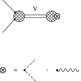
Figure 2: The general single vector meson exchange graph attached to baryons (straight lines) and pions (dashed lines) or external sources (wiggly lines) like e.g. the photon. The shaded areas denote the loop expansion of the respective vertices. Notice that the circle-cross is completely embedded in the shaded area on the right.

There is no a priori reason why multi–loop graphs can not even modify the lowest order results, see also ref.[1]. We will now show that in the tensor and in the vector formulation, these type of graphs only contribute to subleading orders, i.e. they do neither modify the Weinberg term nor the leading contributions to the anomalous magnetic moments of the octet baryons. This is intimately related to the form of the $V\phi\phi$ and $V_{\mu}A^{\mu}$ couplings.

Consider first the vector formulation. The two–pion–vector vertex is proportional to

$$(p^{\prime}-p)_{\nu}\,(k+p^{\prime}-p)^{\nu}\,k^{\mu}$$ (53)

Figure 3: Momentum flow in the $V\phi\phi$–vertex.

where the vector carries momentum $p^{\prime}-p$ and the in–coming (out–going) pion $k$ ($k+p^{\prime}-p$), see Fig.3. This obviously vanishes in forward direction, $p^{\prime}\to p$. Similarly, the photon–vector meson vertex is proportional to $(p^{\prime}-p)_{\nu}(p^{\prime}-p)_{\mu}$, which is at least of order $q^{2}$ and thus can not contribute to the leading order anomalous magnetic moment term. In the tensor field formulation, the vector–two–pion vertex is proprtional to

$$k_{\mu}\,(k+p^{\prime}-p)_{\nu}=k_{\mu}\,(p^{\prime}-p)_{\nu}\,\,\,,$$ (54)

for the same routing of momenta as above and we have made use of the antisymmetry of the tensor field propagator under $\mu\leftrightarrow\nu$ interchange. Thus, there is no contribution to the Weinberg term but only to subleading corrections. The eventual differences appearing in these subleading orders can be absorbed by proper redefinitions of the LECs $(G,H\ldots,T,U)_{D/F}$.

6 Short Summary

In this paper, we have considered the coupling of massive spin–1 fields to the effective field theory of the Goldstone bosons and the ground state baryon octet. The corresponding Lagrangian is parametrized beyond leading order in terms of so–called low–energy constants. These can be estimated by $s$–channel baryonic and $t$–channel mesonic excitations. For the latter type of contributions, massive spin–1 fields (in particular vector mesons) play an important role. If one does not assume any particular underlying dynamics for these fields but only their transformation properties under non–linearly realized chiral symmetry, one is left with two possibilities, namely to represent the three degrees of freedom by a conventional vector or a properly constrained antisymmetric tensor field. One expects these two representations to be equivalent. That is indeed what we have shown here. For that, we have constructed the effective action of the Goldstone boson–baryon-spin–1 system for both types of spin–1 representations. These in general differ by local (contact) terms with a priori undetermined coefficients. The study of the baryon electromagnetic form factors allowed us to pin down these local terms, which have to be added in the vector field formulation, and to determine their corresponding coefficients. We also clarified the situation concerning the so–called Weinberg term of relevance to low energy pion–nucleon scattering. In the approach discussed here, it arises from the chiral covariant derivative acting on the baryons and not from vector meson exchange. The latter type of process contributes at next–to–leading order, as specifed above. In summary, the situation is very similar to the one in the meson sector were some local contact terms of dimension four have to be added in case of the vector field approach to achieve e.g. a satisfactory description of the pion electromagnetic form factor at next–to–leading order [10] (or, to be precise, the electromagnetic radius of the pion). Finally, we have briefly discussed some problems related to loops in the presence of massive particles. These, however, do not alter any of our conclusions.

Appendix A Construction Principles

Here, we collect a few useful formulae which are needed to construct the effective Lagrangians ${\cal L}^{(1)}_{B\phi W}$ and ${\cal L}^{(1)}_{B\phi V}$. To the order we are working, we can make use of the equation of motion for the baryon fields derived from ${\cal L}^{(1)}_{B\phi}$

$$i\gamma^{\mu}[D_{\mu},B]-mB+\frac{1}{2}D\gamma^{\mu}\gamma_{5}\{u_{\mu},B\}+\frac{1}{2}F\gamma^{\mu}\gamma_{5}[u_{\mu},B]=0\,\,.$$ (A.1)

In fact, only the chiral–covariant kinetic and the mass terms will be of relevance to the order we are working. It is worth to stress that we only consider processes with at most two external pions or one external vector source, like e.g. single vector–meson exchange in Goldstone boson–baryon scattering or $t$–channel vector meson exciations contributing to the baryon electromagnetic form factors. It is straightforward to generalize our considerations to more complicated processes. In what follows, we frequently employ our short–hand notation $(A,B)$ meaning either $[A,B]$ or $\{A,B\}$.

Consider first the tensor field formulation. We want to construct terms which contain one antisymmetric tensor and at most two covariant derivatives since in the low energy domain

$$[D_{\mu},[D_{\nu},W_{\lambda\kappa}]]={\cal O}(q^{2})\,\,\,.$$ (A.2)

Because of the antisymmetry of $W_{\mu\nu}$, many terms vanish. We give one example

$${\rm Tr}\,\biggl{[}\bar{B}\biggl{(}[D^{\mu},[D^{\nu},W_{\mu\nu}]\,,\,B\biggr{)}\biggr{]}\sim{\rm Tr}\,\biggl{[}\bar{B}\biggl{(}[u^{\mu},u^{\nu}],W_{\mu\nu}]\,,\,B\biggr{)}\biggr{]}=0\,\,\,,$$ (A.3)

for the processes under consideration. The term on the right–hand–side of Eq.(A.3) gives rise to e.g. a vector-two-pion-baryon seagull term and is thus of no relevance here. The discrete symmetries $P$, $C$ and $T$ as well as hermiticity and Lorentz and chiral invariance strongly constrain the possible terms. Consider e.g. charge conjugation. We have

$$C:\quad W_{\mu\nu}^{c}=-W_{\mu\nu}^{T}\,\,,\,B^{c}=C\,\bar{B}^{T}\,\,,\,\bar{B}^{c}=B^{T}\,C\,\,,\,D_{\mu}^{c}=-D_{\mu}^{T}\,\,,$$ (A.4)

and the standard transformation properties for the Dirac matrices. This eliminates for example a term like

$${\rm Tr}\,\biggl{[}\bar{B}\gamma^{\mu}\biggl{(}D^{2}W\,,\,D^{3}B\biggr{)}\biggr{]}^{c}\simeq-{\rm Tr}\,\biggl{[}\bar{B}\gamma^{\mu}\biggl{(}(D^{2},W)\,,\,D^{3}B\biggr{)}\biggr{]}\,\,\,,$$ (A.5)

in symbolic notation (i.e. dropping all unnecessary indices). The ’$\simeq$’ means that we have dropped terms of higher order which arise when one moves the covariant derivatives around. Under parity transformations

$$P: \quad P\,W_{\mu\nu}(x)\,P^{\dagger}=W^{\mu\nu}(\tilde{x})\,\,,\,P\,D_{\mu}(x)\,P^{\dagger}=D^{\mu}(\tilde{x})\,\,,$$ (A.6)

$$\quad P\,B(x)\,P^{\dagger}=\gamma_{0}\,B(\tilde{x})\,\,,\,P\,\bar{B}(x)\,P^{\dagger}=\bar{B}(\tilde{x})\,\gamma_{0}\,\,\,,$$

with $\tilde{x}^{\mu}=x_{\mu}$. We also note that while $W_{\mu\nu}$ is hermitean, $W_{\mu\nu}^{\dagger}=W_{\mu\nu}$, the covariant derivative is anti-hermitean, $D_{\mu}^{\dagger}=-D_{\mu}$. With these tools at hand, one readily constructs the effective Lagrangian Eq.(19).

For the vector field formulation, one can proceed similarly. Here, however, it is helpful to remember the standard $\rho$–meson–nucleon vector and tensor couplings,

$${\cal L}_{\rho N}=\frac{g}{2}\,\bar{\Psi}_{N}\,\biggl{[}\gamma^{\mu}\,\vec{\rho}_{\mu}\cdot\vec{\tau}-\frac{\kappa_{\rho}}{2m}\,\sigma^{\mu\nu}\,\partial_{\nu}\,\vec{\rho}_{\mu}\cdot\vec{\tau}\biggr{]}\,\Psi_{N}\,\,\,.$$ (A.7)

These terms can easily be transcribed into SU(3) vector meson-baryon couplings (in the vector field formulation) of the type

$${\rm Tr}\,\bigl{[}\bar{B}\,\gamma^{\mu}\,(V_{\mu}\,,\,B)\,\bigr{]}\,\,\quad{\rm and}\quad{\rm Tr}\,\bigl{[}\bar{B}\,\sigma^{\mu\nu}\,(D_{\nu}V_{\mu}\,,\,B)\,\bigr{]}\,\,\,.$$ (A.8)

Furthermore, up to order $q^{4}$ and for diagrams with one baryon line running through, because of momentum conservation we have $[D_{\mu},V^{\mu}]=0$. This argument holds e.g. for elastic forward scattering. More generally, such terms do not contribute to the effective action since

$$\partial^{x}_{\mu}\,\partial^{\lambda,y}\,G_{\nu\lambda}(x)-\partial^{x}_{\nu}\,\partial^{\lambda,y}\,G_{\mu\lambda}(x)=0\,\,\,$$ (A.9)

This condition eliminates a large class of possible terms. To arrive at the terms shown in Eq.(31), one makes use of the antisymmetry of $V_{\mu\nu}$ and uses the equations of motion to let the covariant derivative act on the baryon fields as much as possible. Of course, the discrete symmetries, hermiticity and so on have to be obeyed. These are more standard in the vector field formulation and we thus refrain from discsussing these in detail here.

The last point we want to address are the terms in ${\cal L}_{B\phi V}$ which contain the symmetric tensor $\bar{V}_{\mu\nu}$. One example is the last term in Eq.(31), another such term is e.g. given by

$${\rm Tr}\,\biggl{[}\bar{B}\,\gamma^{\mu}\,\biggl{(}[D_{\lambda},\bar{V}_{\mu\nu}]\,,\,[D^{\lambda},[D^{\nu},B]]\,\biggl{)}\biggl{]}\,\,.$$ (A.10)

In the effective action, it leads to the following four–point function (to be precise, the derivative of it),

$$-i\,\Delta^{\dagger}_{\mu\nu,\rho\sigma}(x,y)=$$ (A.11)

$$\partial^{x}_{\nu}\,\partial^{y}_{\sigma}\,G_{\mu\rho}(x,y)+\partial^{x}_{\nu}\,\partial^{y}_{\rho}\,G_{\mu\sigma}(x,y)-\partial^{x}_{\mu}\,\partial^{y}_{\sigma}\,G_{\nu\rho}(x,y)-\partial^{x}_{\mu}\,\partial^{y}_{\rho}\,G_{\nu\sigma}(x,y)$$

$$= -i\int\frac{d^{4}k}{(2\pi)^{4}}\frac{{\rm e}^{-ik\cdot(x-y)}}{k^{2}-M_{V}^{2}+i\epsilon}\,\biggl{\{}g_{\mu\rho}k_{\nu}k_{\sigma}+g_{\mu\sigma}k_{\nu}k_{\rho}-g_{\nu\rho}k_{\mu}k_{\sigma}-g_{\nu\sigma}k_{\mu}k_{\rho}\,\biggr{\}}\,\,,$$

which is symmetric under $\rho\leftrightarrow\sigma$. Therefore, such a term or the last one in Eq.(31) do not seem to have analoga in the antisymmetric tensor field formulation. If that were to be true, then already at tree level one would have an inequivalence between the two representations for the massive spin–1 fields starting at order ${\cal O}(q^{4})$. However, setting (see also appendix B)

$$V_{\nu}=-\frac{1}{M_{V}^{2}}\,D^{\lambda}\,V_{\lambda\nu}$$ (A.12)

one can rewrite $\bar{V}_{\mu\nu}$ in the following way

$$\bar{V}_{\mu\nu}=-\frac{1}{M_{V}^{2}}\,\bigl{(}D_{\mu}\,D^{\lambda}\,V_{\lambda\nu}+D_{\nu}\,D^{\lambda}\,V_{\lambda\mu}\,\bigr{)}\,\,\,.$$ (A.13)

This latter object is up to an irrelevant prefactor similar to the tensor field combination

$$D_{\mu}\,D^{\lambda}\,W_{\lambda\nu}+D_{\nu}\,D^{\lambda}\,W_{\lambda\mu}\,\,\,\,,$$ (A.14)

which after using the equations of motion for $W_{\mu\nu}$ can be recast into the form

$$2D_{\mu}\,D^{\lambda}\,W_{\lambda\nu}+M_{V}^{2}\,W_{\mu\nu}\,\,\,\,.$$ (A.15)

Consequently, if we decompose $\bar{V}_{\mu\nu}$ as

$$\bar{V}_{\mu\nu}=2\,D_{\mu}\,V_{\nu}-V_{\mu\nu}\,\,\,\,,$$ (A.16)

one realizes that the seemingly inequivalent terms containing the symmetric tensor $\bar{V}_{\mu\nu}$ are also appearing in the tensor field formulation for appropriate combinations of $W_{\mu\nu}$ and the covariant derivatives (like e.g. given in Eq.(A.15)).

Appendix B On the Equivalence from Dual Transformations

Here, we wish to critically examine the approach of Ref.[13], were it was argued that the equivalence between the tensor and vector field formulations can be shown formally by using path integral methods and a set of dual transformations as motivated by e.g. Refs.[26],[27]. The starting point of Ref.[13] is the generating functional in the presence of Goldstone bosons and external vector and axial–vector sources,

$${\cal Z}[u_{\mu},f^{+}_{\mu\nu}]=\int[DV_{\mu}]\,\delta(\partial_{\mu}V^{\mu}){\rm e}^{i\int d^{4}x\,{\cal L}_{V}}\,\,\,,$$ (B.1)

where ${\cal L}_{V}$ denotes the meson Lagrangian of Goldstone bosons chirally coupled to massive spin–1 fields in the vector formulation. First, we wish to examine the role of the $\delta$–function which ensures transversality of the vector field. From the free part of the Lagrangian, Eq.(24), we derive the equation of motion (eom), the well–known Proca equation,

$$\Box\,V_{\nu}^{a}-\partial_{\nu}\,(\partial\cdot V^{a})+M_{V}^{2}\,V_{\nu}^{a}=0\,\,\,,$$ (B.2)

which for $M_{V}\neq 0$ clearly leads to the transversality condition, $\partial\cdot V^{a}=0$. Let us now examine the generating functional more closely. Denote by $V_{\mu}^{0}$ the field which fulfills the equation of motion (we drop the flavor index ${}^{\prime}a^{\prime}$). One finds for the effective action expanded aroung the classical solution

$$S[V_{\mu}] = \int d^{4}x\,{\cal L}_{V}=S[V_{\mu}^{0}]+\int d^{4}x\,(V_{\mu}-V_{\mu}^{0})\,\frac{\delta S}{\delta V_{\mu}}\biggl{|}_{V_{\mu}^{0}}$$ (B.3)

$$+ \frac{1}{2}\,\int d^{4}x\,d^{4}y\,(V_{\mu}-V_{\mu}^{0})(x)\,(V_{\nu}-V_{\nu}^{0})(y)\,\frac{\delta^{2}S}{\delta V_{\mu}\delta V_{\nu}}(x,y)\biggr{|}_{V_{\mu}^{0}}\,\,,$$

which using the eom leads to the generating functional

$${\cal Z}[u_{\mu},f^{+}_{\mu\nu}]=\exp\bigl{(}iS[V_{\mu}^{0}]\bigr{)}\,{\rm det}({\cal M})^{-1/2}\,\,\,,$$ (B.4)

with ${\cal M}=(-i/2)[(\Box+M_{V}^{2})g^{\mu\nu}-\partial^{\mu}\partial^{\nu}]$. Neglecting loops with spin–1 mesons, we have det$\,{\cal M}=1$ and arrive at

$${\cal Z}[u_{\mu},f^{+}_{\mu\nu}]=\exp\bigl{(}iS[V_{\mu}^{0}]\bigr{)}=\int[DV_{\mu}]\,\delta(V_{\mu}-V_{\mu}^{0})\,{\rm e}^{i\int d^{4}x\,{\cal L}_{V}}\,\,\,,$$ (B.5)

which differs from Eq.(B.1) by the argument of the $\delta$–function. To further sharpen this constrast, let us perform the following substitution

$$V^{\mu}\to{V^{\mu}}^{\prime}=V^{\mu}+\frac{f_{V}}{\sqrt{2}M_{V}^{2}}\partial_{\nu}f_{+}^{\nu\mu}+\frac{ig_{V}}{\sqrt{2}M_{V}^{2}}\partial_{\nu}[u^{\nu},u^{\mu}]\,\,\,,$$ (B.6)

which also defines a transverse field and differs in the eom from the original one by terms of order ${\cal O}(q^{5})$ (and higher). To the order we are working and for the processes we are considering, one has

$${\cal L}(V_{\mu})={\cal L}({V_{\mu}}^{\prime})$$ (B.7)

so that the generating functional can also be cast in the form

$${\cal Z}[u_{\mu},f^{+}_{\mu\nu}]=\int[DV_{\mu}]\,\delta\bigl{(}(\Box+M_{V}^{2})\,V_{\mu}-\partial_{\mu}\partial\cdot V\bigr{)}\,{\rm e}^{i\int d^{4}x\,{\cal L}_{V}}\,\,\,.$$ (B.8)

The two representations, Eq.(B.5) and Eq.(B.8), are obviously equivalent as long as $V_{\mu}$ and $V_{\mu}^{\prime}$ fulfill the respective eom. This also ensures tranversality. However, the argument can not be reversed, not any field which obeys $\partial\cdot V=0$ is a solution of the eom. This is in contrast to the starting point of Ref.[13], Eq.(B.1).

We can also make contact to the tensor field formulation. We observe that

$$\delta\bigl{(}(\Box+M_{V}^{2})\,V_{\mu}-\partial_{\mu}\partial\cdot V\bigr{)} = \delta(\partial^{\nu}V_{\nu\mu}+M_{V}^{2}\,V_{\mu})$$ (B.9)

$$\sim \delta\biggl{(}V_{\mu}+\frac{1}{M_{V}^{2}}\,\partial^{\lambda}\,V_{\lambda\mu}\biggr{)}\,\,\,.$$

Consider now $V_{\mu\nu}$ as the fundamental degree of freedom (instead of $V_{\mu}$). This leads to the following generating functional

$$\exp\,\bigl{(}-i\,S[V^{0}_{\mu\nu}]\,\bigr{)}=\int[DV_{\mu}]\,\delta\biggl{(}V_{\mu}+\frac{1}{M_{V}^{2}}\,\partial^{\lambda}\,V_{\lambda\mu}\biggr{)}\,{\rm e}^{-i\int d^{4}x\,{\cal L}_{V}}\,\,,$$ (B.10)

with (it is straightforward to generalize this argument and include the covariant instead of the partial derivative, $\partial_{\mu}\to D_{\mu}$)

$${\cal L}[V_{\mu\nu}]=-\frac{1}{4}{\rm Tr}\,\biggl{(}V_{\mu\nu}V^{\mu\nu}\biggr{)} + \frac{1}{2M_{V}^{2}}\,{\rm Tr}\,\biggl{(}D_{\lambda}V^{\lambda\mu}D^{\rho}V_{\rho\mu}\biggr{)}-{\rm Tr}\,\biggl{(}V_{\mu\nu}\,J^{\mu\nu}\biggr{)}\,.$$

We make the field redefinition

$$\tilde{W}_{\mu\nu}\equiv\frac{1}{M_{V}}\,V_{\mu\nu}$$ (B.12)

where $\tilde{W}_{\mu\nu}$ fulfills the following eom,

$$\partial^{\mu}\,\biggl{\{}\partial_{\mu}\partial^{\rho}\,\tilde{W}_{\rho\nu}-\partial_{\nu}\partial^{\rho}\,\tilde{W}_{\rho\mu}+M_{V}^{2}\,\tilde{W}_{\mu\nu}\,\biggr{\}}=0\,\,\,.$$ (B.13)

The term in the curly brackets is nothing but the eom for the antisymmetric tensor field, cf. the appendix of Ref.[9]. This can be used to show the formal (symbolic) equivalence

$${\cal Z}[u_{\mu},f^{+}_{\mu\nu}]=\exp\,\bigl{(}\,i\,S[V_{\mu}^{0}]\,\bigr{)}=\exp\,\bigl{(}\,i\,S^{\prime}[\tilde{W}_{\mu\nu}^{0}]\,\bigr{)}\,\,\,,$$ (B.14)

provided one substitutes the vector field and its respective field strength tensor in the Lagrangian as follows

$${\cal L}_{V}[V_{\mu},V_{\mu\nu}]\to-{\cal L}_{V}\biggl{[}-\frac{1}{M_{V}}D^{\lambda}\tilde{W}_{\lambda\mu},M_{V}\,\tilde{W}_{\mu\nu}\biggr{]}\,\,\,.$$ (B.15)

Therefore, the rather conventional treatment of the path integral presented here leads to

$${\cal Z}[u_{\mu},f^{+}_{\mu\nu}]=\int[DV_{\mu}]\,\delta\biggl{(}\,V_{\mu}+\frac{1}{M_{V}^{2}}\,D^{\lambda}V_{\lambda\mu}\,\biggr{)}\,{\rm e}^{\,i\int d^{4}x\,{\cal L}_{V}}\,\,\,.$$ (B.16)

In Ref.[13], an extra integration over the field $H_{\mu\nu}$, $\int[DH_{\mu\nu}]$, is performed. This additional integration allows to produce additional constant terms in the Goldstone boson–spin–1 Lagrangian and is at the heart of the formal equivalence. However, the coefficients of the local contact terms can only be fixed since it is known that the tensor formulation indeed gives the correct result (for e.g. the pion radius). We remark here that in the papers on dual transformations, the components of the field strength tensor are in general not treated as a degrees of freedom independent of the vector field components. Let us summarize our observations. Starting from Eq.(B.16) and considering $V_{\mu\nu}$ as the fundamental object, we could introduce (by rescaling) the field ${\tilde{W}}_{\mu\nu}$ which obeys the eom of the antisymmetric tensor field. Furthermore, the Lagrangian can be shown to be identical to the one in tensor field formulation. This allows to identify ${\tilde{W}}_{\mu\nu}$ with the fundamental antisymmetric tensor field $W_{\mu\nu}$ up to an overall constant which can be absorbed in the coupling constants appearing in the current $J_{\mu\nu}$. This equivalence is, however, formal. The complete equivalence as discussed in Ref.[13] can only be achieved if one treats the vector field $V_{\mu}$ and the vector $D^{\rho}H_{\rho\mu}$ appearing in the dual transfomation as independent degrees of freedom. Again, this does not fix the coefficients of the local contact terms, for doing that, arguments like in Ref.[10] have to be invoked.

References

- [1] J. Gasser, M.E. Sainio and A. varc, Nucl. Phys. B307 (1988) 779
- [2] E. Jenkins and A.V. Manohar, Phys. Lett. B255 (1991) 558
- [3] E. Jenkins and A.V. Manohar, in “Effective Field Theories of the Standard Model”, ed. Ulf-G. Meißner, World Scientific, Singapore, 1992
- [4] V. Bernard, N. Kaiser, J. Kambor and Ulf-G. Meißner, Nucl. Phys. B388 (1992) 315
- [5] V. Bernard, N. Kaiser and Ulf-G. Meißner, Int. J. Mod. Phys. E4 (1995) 193
- [6] S. Weinberg, Physica 96A (1979) 327
- [7] J. Gasser and H. Leutwyler, Ann. Phys. (N.Y.) 158 (1984) 142
- [8] J. Gasser and H. Leutwyler, Nucl. Phys. B250 (1985) 465
- [9] G. Ecker, J. Gasser, A. Pich and E. de Rafael, Nucl. Phys. B321 (1989) 311
- [10] G. Ecker, J. Gasser, H. Leutwyler, A. Pich and E. de Rafael, Phys. Lett. B223 (1989) 425
- [11] J.F. Donoghue, C. Ramirez and G. Valencia, Phys. Rev. D39 (1989) 1947
- [12] Ulf-G. Meißner, Phys. Rep. 161 (1988) 213
- [13] J. Bijnens and E. Pallante, preprint NORDITA-95/63 [hep-ph/9510338]
- [14] G. Ecker, Phys. Lett. B336 (1994) 508
- [15] G. Ecker and M. Mojzis, Wien preprint UWThPh-1995-22 [hep-ph/9508204]
- [16] A. Krause, Helv. Physica Acta 63 (1990) 3
- [17] S. Weinberg, Phys. Rev. 166 (1968) 1568
- [18] V. Bernard, N. Kaiser and Ulf-G. Meißner, Phys. Lett. B309 (1993) 421
- [19] V. Bernard, N. Kaiser and Ulf-G. Meißner, Nucl. Phys. B457 (1995) 147
- [20] Ulf-G. Meißner, in “Chiral Dynamics: Theory and Experiment”, A.M. Bernstein and B.R. Holstein (eds.), Springer, Berlin, 1995
- [21] Ulf-G. Meißner, Int. J. Mod. Phys. E1 (1992) 561
-
[22]
K. Kawarabayashi and M. Suzuki, Phys. Rev. Lett. 16 (1966) 255;
Fayyazuddin and Riazuddin, Phys. Rev. 147 (1966) 1071 - [23] V. Bernard, N. Kaiser and Ulf-G. Meißner, Z. Phys. C60 (1993) 111
- [24] M. Bando, T. Kugo and K. Yamawaki, Phys. Rep. 164 (1988) 217
- [25] P. Mergell, Ulf-G. Meißner and D. Drechsel, preprint MKPH-T-95-07 and TK 95-15, 1995, Nucl. Phys. A (in print) [hep-ph/9506375]
- [26] P.K. Townsend, K. Pilch and P. van Nieuwenhuizen, Phys.Lett. B136 (1984) 38
- [27] S. Deser and R. Jackiw, Phys.Lett. B139 (1984) 371