Semi-Inclusive Deeply Inelastic Scattering at Small ${q_{T}}$

Abstract

Measurement of the distribution of hadronic energy in the final state in deeply inelastic electron scattering at HERA can provide a good test of our understanding of perturbative QCD. For this purpose, we consider the energy distribution function, which can be computed without needing final state parton fragmentation functions. We compute this distribution function for finite transverse momentum ${q_{T}}$ at order $\alpha_{s}$, and use the results to sum the perturbation series to obtain a result valid for both large and small values of transverse momentum.

I Introduction

This paper concerns the energy distribution in the final state of deeply inelastic lepton scattering. Using a naive parton model, one would predict that the scattered parton appears as a single narrow jet at a certain angle $(\theta_{*},\phi_{*})$ in the detector. Taking hard QCD interactions into account, one predicts a much richer structure for the final state energy distribution. In a previous paper${}^{\cite[cite]{[\@@bibref{Number}{mos}{}{}]}}$ (henceforth referred to as I), we investigated this structure, using an energy distribution function defined in analogy to the energy-energy correlation function in $e^{+}e^{-}$ annihilation.${}^{\cite[cite]{[\@@bibref{Number}{energycor,ellis}{}{}]}}$ We studied this energy distribution as a function of angle $(\theta_{B},\phi_{B})$ in the detector in the region not too near to the direction $(\theta_{*},\phi_{*})$. In this region, simple QCD perturbation theory is applicable, and we presented calculations at order $\alpha_{s}$. In this paper, we extend the analysis to the region of $(\theta_{B},\phi_{B})$ near to $(\theta_{*},\phi_{*})$ . Here, multiple soft gluon radiation is important. Thus we use a summation of perturbation theory.

A The energy distribution function

There is extensive literature on semi-inclusive deeply inelastic scattering;${}^{\cite[cite]{[\@@bibref{Number}{early,late,todd,mirkes,graudenz,peccei,morfin}{}{}]}}$ a brief history and complete set of references can be found in paper I. We begin here with a concise review of how the energy distribution function is defined, and then discuss how we sum the contributions that are important in the region $(\theta_{B},\phi_{B})\simeq(\theta_{*},\phi_{*})$ to obtain a result which is valid for all values of $(\theta_{B},\phi_{B})$.

The reaction that we study is $e+{\rm A}\to e+{\rm B}+{\rm X}$ at the HERA electron-proton collider.${}^{\cite[cite]{[\@@bibref{Number}{wsmith}{}{}]}}$ Let us describe the particles by their energies and angles in the HERA laboratory frame, with the positive z-axis chosen in the direction of the proton beam and the negative z-axis in the direction of the electron beam. In completely inclusive deeply inelastic scattering, one measures only $E^{\prime}$ and $\theta^{\prime}$, the energy and angle of the scattered electron. In the semi-inclusive case studied in this paper, one also measures some basic features of the hadronic final state. In principle, one can measure the energy $E_{B}$ and the angles $(\theta_{B},\phi_{B})$ of the outgoing hadron B. However, it is much simpler to perform a purely calorimetric measurement, in which only the total energy coming into a calorimeter cell at angles $(\theta_{B},\phi_{B})$ is measured. This calorimetric measurement gives the energy distribution

$${d\Sigma\over dE^{\prime}\ d\cos\theta^{\prime}\ d\cos\theta_{B}\ d\phi_{B}}=\sum_{B}\int dE_{B}\ (1-\cos\theta_{B})E_{B}\ {d\sigma(e+A\to B+X)\over dE^{\prime}\ d\cos\theta^{\prime}\ dE_{B}\ d\cos\theta_{B}\ d\phi_{B}}\ .$$ (1)

The sum runs over all species of produced hadrons B. We have included a factor $(1-\cos\theta_{B})$ in the definition because this factor is part of the Lorentz invariant dot product $P_{A,\mu}P_{B}^{\mu}=E_{A}E_{B}(1-\cos\theta_{B})$.

Notice that $d\Sigma$ measures the distribution of energy in the final state as a function of angle without asking how that energy is split into individual hadrons moving in the same direction.${}^{\cite[cite]{[\@@bibref{Number}{feynman}{}{}]}}$ For this reason, the theoretical expression for $d\Sigma$ will not involve parton decay functions that describe how partons decay into hadrons.

B Partonic variables and their relation to HERA lab frame

At the Born level, the hard scattering process for the reaction is $electron+quark\to electron+quark$ by means of virtual photon or ${\rm Z}_{0}$ exchange. At order $\alpha_{s}$, one can have virtual corrections to the Born graph. In addition, one can have processes in which there are two scattered partons in the final state. Then the initial parton can be either a quark (or antiquark) or a gluon, while the observed hadron can come from the decay of either of the final state partons. Some of these possibilities are illustrated in Fig. 1, Fig. 2, and Fig. 3.

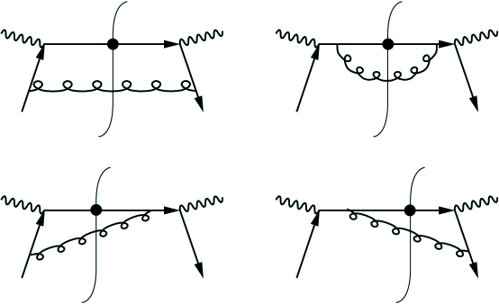
FIG. 1.: Feynman diagrams for quark initiated process with a quark jet observed. The observed parton is the upper line, indicated with a dot.

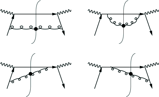
FIG. 2.: Feynman diagrams for quark initiated process with a gluon jet observed. The observed parton is the lower line, indicated with a dot.

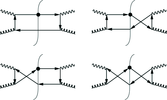
FIG. 3.: Feynman diagrams for gluon initiated process with a quark jet observed. The observed parton is the upper line, indicated with a dot.

Let us consider the effect of the emission of the additional, unobserved, “bremsstrahlung” parton. We can define the part of the vector boson momentum $q^{\mu}$ that is transverse to the momentum of the incoming hadron $P_{A}^{\mu}$ and to the momentum of the outgoing hadron $P_{B}^{\mu}$. One merely subtracts from $q^{\mu}$ its projections along $P_{A}^{\mu}$ and $P_{B}^{\mu}$ (taking $P_{A}^{2}=P_{B}^{2}=0$),

$$q_{T}^{\mu} = q^{\mu}-{\displaystyle{q\cdot P_{B}\over P_{A}\cdot P_{B}}}\,P_{A}^{\mu}-{\displaystyle{q\cdot P_{A}\over P_{A}\cdot P_{B}}}\,P_{B}^{\mu}\quad.$$ (2)

We let ${q_{T}}=[-q_{T}^{\mu}\cdot{{q_{T}}}_{\mu}]^{1/2}$ represent the magnitude of the transverse momentum. It is ${q_{T}}$ that is analogous to the transverse momentum of produced W’s and Z’s or lepton pairs in the Drell Yan process. In the naive parton model, there are no bremsstrahlung partons and all parton momenta are exactly collinear with the corresponding hadron momenta, so one has ${q_{T}}=0$. At order $\alpha_{s}$, unobserved parton emission allows ${q_{T}}$ to be nonzero.

In order to properly describe the parton kinematics we need four more variables besides ${q_{T}}$. Two are the standard variables for deeply inelastic scattering, $Q^{2}=-q^{\mu}q_{\mu}$ and $x=Q^{2}/(2q\cdot P_{A})$. The third is a momentum fraction for the outgoing hadron $B$,

$$z={P_{B}\cdot P_{A}\over q\cdot P_{A}}\qquad.$$ (3)

(Thus the integration over the energy of hadron $B$ in definition (1) of the energy distribution is equivalent to an integration over $z$.) The fourth variable is an azimuthal angle $\phi$. To define $\phi$, we choose a frame, called the hadron frame, Fig. 4, in which the incoming hadron $A$ has its three-momentum $P_{A}$ along the positive $z$-axis and the virtual photon four-momentum $q^{\mu}$ lies along the negative $z$-axis. Then as long as ${q_{T}}\not=0$, hadron $B$ has some transverse momentum, and we align the $x$- and $y$-axes so that $P_{B}^{x}>0$ and $P_{B}^{y}=0$. We now define $\phi$ as the azimuthal angle of the incoming lepton in the hadron frame. These variables are described more fully in paper I, and relevant formulas are given in the Appendix of this paper.

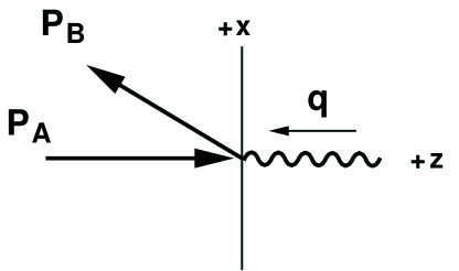
FIG. 4.: The hadron frame. The initial hadron $P_{A}$ lies along the positive $z$-axis, and the vector boson $q$ lies along the negative $z$-axis. The next-to-leading order QCD corrections can give the final state hadron $P_{B}$ a non-zero $x$-component.

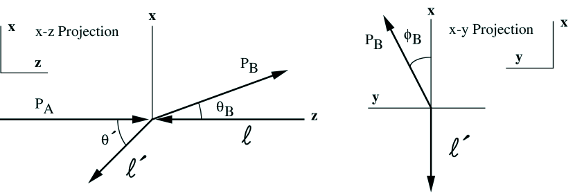
FIG. 5.: The HERA lab frame for the process: $e^{-}(\ell)+A(P_{A})\to e^{-}(\ell^{\prime})+B(P_{B})+X$. The final state leption $e^{-}(\ell^{\prime})$ lies in the $x$-$z$–plane, and the final state hadron $B(P_{B})$ has a non-zero $y$-component if $\phi_{B}$ is non-zero.

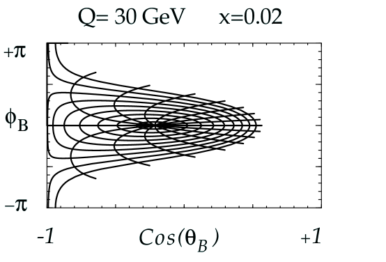
FIG. 6.: Contours in $\phi_{B}$ and $\cos(\theta_{B})$ for $Q=30\,{{\rm GeV}}$ and $x=0.02$. The circular rings are contours of constant ${q_{T}}$ in steps of 3 GeV, and the radial arcs are contours of constant $\phi$ in steps of $\pi/8$.

The variables ${q_{T}}$ and $\phi$ can be translated to the observables of the HERA lab frame, Fig. 5. In the naive parton model, the outgoing hadron $B$ (along with all the other hadrons arising from the decay of the struck quark) emerges in the plane defined by the incoming and outgoing electrons at a precisely defined angle $(\theta_{*},\phi_{*})$, which can be computed from the incoming particle momenta and the momentum of the scattered electron. The point ${q_{T}}=0$ corresponds to $(\theta_{B},\phi_{B})=(\theta_{*},\phi_{*})$. We choose our $x$-axis such that $\phi_{*}=0$. Lines of constant positive ${q_{T}}$ are curves in the $(\theta_{B},\phi_{B})$ plane that encircle the point $(\theta_{*},\phi_{*})$. Lines of constant $\phi$ radiate out of the point $(\theta_{*},\phi_{*})$, crossing the lines of constant ${q_{T}}$. This is illustrated in Fig. 6. The precise formulas for the map relating $(\theta_{B},\phi_{B})$ and $({q_{T}},\phi)$ are given in the Appendix.

In paper I and in this paper, we find it convenient to convert from the laboratory frame variables $\{E^{\prime},\theta^{\prime}\}$ of the scattered lepton and $\{\theta_{B},\phi_{B}\}$ of the observed hadron to $\{x,Q^{2}\}$ for the lepton and $\{{q_{T}},\phi\}$ for the observed hadron. We also convert from $E_{B}$ to $z$. With this change of variables, Eq. (1) becomes

$${d\Sigma\over dx\,dQ^{2}\,d{q_{T}^{2}}\,d\phi}=\sum_{B}\int\,dz\,z\ \left({\displaystyle{Q^{2}\over 2x\,E_{A}}}\right)\ {d\sigma\over dx\,dQ^{2}\,d{q_{T}^{2}}\,d\phi\,dz}\ .$$ (4)

C The Sudakov summation of logarithms of ${q_{T}}$

The main object of study in this paper is the distribution of energy as a function of ${q_{T}}$ for ${q_{T}^{2}}\ll Q^{2}$. In paper I, we applied straightforward perturbation theory to analyze the energy distribution in the region ${q_{T}^{2}}\sim Q^{2}$, and $\alpha_{s}(Q^{2})\ll 1$. Here there is a rich structure as a function of the angles that relate the hadron momenta to the lepton momenta. In fact, a complete description requires nine structure functions.

When one examines the region ${q_{T}^{2}}\ll Q^{2}$, one finds that the angular structure simplifies greatly. However, the dependence on ${q_{T}}$ becomes richer than the dependence on ${q_{T}}$ of the lowest order graphs. By summing the most important parts of graphs at arbitrarily high order, one finds a structure that is sensitive to the fact that QCD is a gauge theory.

Briefly, the physical picture${}^{\cite[cite]{[\@@bibref{Number}{parisi}{}{}]}}$ is as follows. At the Born level of deeply inelastic scattering, a quark in the incoming proton enters the scattering with momentum $\xi P_{A}^{\mu}$ that is precisely along the beam axis. This quark is scattered by a virtual photon, $Z$- or $W$-boson. Its momentum $\xi P_{A}^{\mu}+q^{\mu}$ is in a direction $(\theta_{*},\phi_{*})$ that can be reconstructed by knowing the lepton momenta. However at higher orders of perturbation theory, the momentum of the final state parton is

$$(\xi P_{A}^{\mu}+q^{\mu})-(k_{1}^{\mu}+k_{2}^{\mu}+\cdots+k_{N}^{\mu})\qquad,$$ (5)

where the $k_{i}^{\mu}$ are momenta of gluons that emitted in the process. In a renormalizable field theory, it is very easy to emit gluons that are nearly collinear to either the initial or final parton directions. In addition, in a gauge theory such as QCD, it is very easy to emit gluons that are soft ($k^{\mu}\ll Q$). Each gluon emission displaces ${q_{T}}$ by a small amount, so that one may think of the parton as undergoing a random walk in the space of transverse momenta. With one gluon emission, one finds a cross section that is singular as ${q_{T}}\to 0$:

$${d\sigma\over d\,q_{T}^{2}}\ \propto\ \alpha_{s}\,{a+b\log(q_{T}^{2}/Q^{2})\over q_{T}^{2}}\ .$$ (6)

At order $\alpha_{s}^{N}$ the $1/q_{T}^{2}$ singularity is multiplied by a polynomial in $\log(q_{T}^{2}/Q^{2})$ of order $2N-1$. This series sums to a function of $q_{T}$ that is peaked at $q_{T}=0$ but is not singular there. The width of this distribution is much bigger than the $300\ {\rm MeV}$ that one would guess based on experience with soft hadronic physics. On the other hand the width is quite small compared to the hard momentum scale $Q$.

Essentially this same physics has been studied in the two crossed versions of the process $e+A\to e+B+X$ that can be studied at HERA. In electron-positron annihilation, $e+\bar{e}\to A+B+X$, one looks at the energy-energy correlation function for hadrons $A$ and $B$ nearly back-to-back.${}^{\cite[cite]{[\@@bibref{Number}{CSS,eedata,LEPSLC}{}{}]}}$ In $A+B\to\ell+\bar{\ell}+X$, one studies the distribution of the lepton pair as a function of its transverse momentum $q_{T}$ with respect to the beam axis.${}^{\cite[cite]{[\@@bibref{Number}{CSS,DWS,drellyan,qiu,fnalexp,naexp,MirkesOhnemus}{}{}]}}$ The same analysis applies also to the distribution of the transverse momentum of $W$ or $Z$ bosons produced in hadron colliders.${}^{\cite[cite]{[\@@bibref{Number}{altarelliwzpt,wzpt,ArnoldKauffman,yuanladinsky}{}{}]}}$

From these studies, the following picture emerges. First, the leading logs ($n=2N-1$) can be summed to all orders, and dominate the perturbation theory in the region $\alpha_{s}(Q^{2})\ll 1$ and $\alpha_{s}(Q^{2})\,\ln^{2}(Q^{2}/{q_{T}^{2}}){\lower 2.15277pt\hbox{$\stackrel{{\scriptstyle<}}{{\sim}}$}}1$. Unfortunately, most of the interesting physics, and most of the data, lie outside this region of validity of the leading logarithm approximation. Fortunately, one can go beyond the leading logarithm summation to obtain a result that is valid even when $\alpha_{s}(Q^{2})\ln^{2}(Q^{2}/{q_{T}^{2}})$ is large.${}^{\cite[cite]{[\@@bibref{Number}{CSS,ArnoldKauffman}{}{}]}}$

The plan for the remainder of the paper is as follows. In Sec. 2, we use our $\alpha_{s}$ calculation in paper I to calculate the asymptotic form of the energy distribution functions in the ${q_{T}}\to 0$ limit. In Sec. 3, we introduce the Sudakov form factor which sums the soft gluon radiation in the limit ${q_{T}}\to 0$. In Sec. 4, we compare the asymptotic form of the energy distribution functions to extract the order $\alpha_{s}$ contributions to the perturbative coefficients $A$, $B$, $C^{\rm IN}$ and $C^{\rm OUT}$. In Sec. 5, we address the issue of matching the small ${q_{T}}$ region to the large ${q_{T}}$ region. In Sec. 6 we investigate the form of the non-perturbative corrections in the small ${q_{T}}$ region, and relate these to the Drell-Yan and $e^{+}e^{-}$ processes. In Sec. 7, we review the principle steps in the calculation. In Sec. 8, we present results for the energy distribution functions throughout the full ${q_{T}}$ range. Conclusions are presented in Sec. 9, and the Appendix contains a set of relevant formulas.

II The Energy Distribution Functions

In this section we review the order $\alpha_{s}$ perturbative results of paper I in order to extract the terms in $d\Sigma/dx\,dQ^{2}\,dq_{T}^{2}\,d\phi$ that behave like $1/q_{T}^{2}$ times logs as $q_{T}\to 0$. In Sec. 3, we display the structure of $d\Sigma/dx\,dQ^{2}\,dq_{T}^{2}\,d\phi$ with the Sudakov summation of logarithms. Then in Sec. 4, by comparing the summed form with the order $\alpha_{s}$ form of $d\Sigma/dx\,dQ^{2}\,dq_{T}^{2}\,d\phi$, we will be able to extract the coefficients that appear in the summed form.

A Energy Distribution Formulas

The process we consider is $e^{-}+A\to e^{-}+B+X$, and the fundamental formula for the energy distribution is:

$${d\Sigma\over dx\,dQ^{2}\,d{q_{T}^{2}}\,d\phi} = \sum_{k=1}^{9}\ {\cal A}_{k}(\psi,\phi)\sum_{V_{1},V_{2}}\ \sum_{j,j^{\prime}}\ \Sigma_{0}(Q^{2};V_{1},V_{2},j,j^{\prime},k)\ \Gamma_{k}(x,Q^{2},q_{T}^{2};j,j^{\prime})\qquad.$$ (7)

The hyperbolic boost angle, $\psi$, that connects the natural hadron and lepton frame is given by${}^{\cite[cite]{[\@@bibref{Number}{angulartheory}{}{}]}}$

$${{\rm cosh}}\psi = \frac{2xs}{Q^{2}}-1\qquad,$$ (8)

and $\phi$ is the azimuthal angle in the hadron frame. The nine angular functions ${\cal A}_{k}(\psi,\phi)$ arise from hyperbolic $D^{1}(\psi,\phi)$ rotation matrices. The complete set of ${\cal A}_{k}(\psi,\phi)$ are listed in the Appendix, but the two we shall focus on are

$${\cal A}_{1}(\psi,\phi) = 1+{{\rm cosh}}^{2}(\psi)$$ (9)

$${\cal A}_{6}(\psi,\phi) = 2\ {{\rm cosh}}(\psi)\qquad.$$ (10)

We sum over the intermediate vector bosons $\{V_{1},V_{2}\}=\{\gamma,Z^{0}\}$ or $\{W^{\pm}\}$, as appropriate, and we also sum over the initial and final partons, $\{j,j^{\prime}\}$. The factor $\Sigma_{0}(Q^{2};V_{1},V_{2},j,j^{\prime},k)$ contains the leptonic and partonic couplings, the boson propagators, and numerical factors; it is defined in the Appendix, Eq. (B2). It is the hadronic energy distribution functions, $\Gamma_{k}(x,Q^{2},q_{T}^{2};j,j^{\prime})$, that we shall calculate.

If we expand the $\Gamma_{k}$ in the form of perturbative coefficients convoluted with parton distribution functions, then two of the functions $\Gamma_{k}$, namely $\Gamma_{1}$ and $\Gamma_{6}$, behave like $\log^{n}({q_{T}^{2}}/Q^{2})/{q_{T}^{2}}$ with $n\geq 0$ for ${q_{T}}\to 0$. The others behave like $1/{q_{T}}$ or $1$ times possible logarithms. In this paper we are interested in small ${q_{T}}$ behavior, so we concentrate our attention on $\Gamma_{1}$ and $\Gamma_{6}$.

What of the less singular structure functions $\Gamma_{2}$, $\Gamma_{3}$, $\Gamma_{4}$, $\Gamma_{5}$, $\Gamma_{7}$, $\Gamma_{8}$ and $\Gamma_{9}$? Fixed order perturbation theory is not applicable for the calculation of these $\Gamma_{k}$ for small $q_{T}$. We note, on the grounds of analyticity, that these $\Gamma_{k}$ must be finite or, for certain $k$, vanish as $q_{T}\to 0$, even though they have weak singularities in finite order perturbation theory. Our perturbative results in the region of moderate $q_{T}$ indicate that the fraction of $d\Sigma/dx\,dQ^{2}\,dq_{T}^{2}\,d\phi$ contributed by these $\Gamma_{k}$ is small and dropping as $q_{T}$ decreases. We thus conclude that these contributions would be hard to detect experimentally for small $q_{T}$. For this reason, we do not address the problem of summing perturbation theory for $\Gamma_{2}$, $\Gamma_{3}$, $\Gamma_{4}$, $\Gamma_{5}$, $\Gamma_{7}$, $\Gamma_{8}$ and $\Gamma_{9}$.

Applying the methods of Refs. [28, 14] to deeply inelastic scattering, we write $\Gamma_{1}$ in the form

$$\Gamma_{1}(x,Q^{2},{q_{T}^{2}};j,j^{\prime}) = \Gamma_{1}^{Pert}(x,Q^{2},{q_{T}^{2}};j,j^{\prime})-\Gamma_{1}^{Asym}(x,Q^{2},{q_{T}^{2}};j,j^{\prime})+W(x,Q^{2},q_{T}^{2};j,j^{\prime})\quad.$$ (11)

Here $W(x,Q^{2},q_{T}^{2};j,j^{\prime})$ sums the singular terms to all orders, and contains the leading behavior of $\Gamma_{1}$ as ${q_{T}}\to 0$. $\Gamma_{1}^{Pert}(x,Q^{2},{q_{T}^{2}};j,j^{\prime})$ is simply $\Gamma_{1}(x,Q^{2},{q_{T}^{2}};j,j^{\prime})$ evaluated at a finite order ($\alpha_{s}^{1}$ for our purpose) in perturbation theory. $\Gamma_{1}^{Asym}(x,Q^{2},{q_{T}^{2}};j,j^{\prime})$ equals $W(x,Q^{2},q_{T}^{2};j,j^{\prime})$ truncated at a finite order of $\alpha_{s}$ in perturbation theory. Specifically, if we expand $W(x,Q^{2},q_{T}^{2};j,j^{\prime})$ in the form of perturbative coefficients convoluted with parton distribution functions, then the coefficients have the form of $\log^{n}({q_{T}^{2}}/Q^{2})/{q_{T}^{2}}$ with $n\geq 0$. There are, by definition, no terms that behave like $({q_{T}^{2}}/Q^{2})^{p}$ times possible logarithms for $p>-1$. Such terms exist in $\Gamma_{1}$, but they are associated with $(\Gamma_{1}^{Pert}-\Gamma_{1}^{Asym})$ in Eq. (LABEL:eq:smallqTdecompose).

The angular function ${\cal A}_{1}(\psi,\phi)=1+{{\rm cosh}}^{2}(\psi)$ that multiplies $W$ in the small ${q_{T}}$ limit arises from the numerator factor

$${\rm Tr}\{{{\ell\kern-4.6pt\raise 2.0pt\hbox{/}}}\gamma_{\mu}{{\ell\kern-4.6pt\raise 2.0pt\hbox{/}}}^{\prime}\gamma_{\nu}\}\ {\rm Tr}\{{{P\kern-6.5pt\raise 2.0pt\hbox{/}}}_{\!\!A}\gamma^{\mu}{{P\kern-6.5pt\raise 2.0pt\hbox{/}}}_{\!\!B}\gamma^{\nu}\}\qquad.$$ (13)

Here ${\rm Tr}\{{{\ell\kern-4.6pt\raise 2.0pt\hbox{/}}}\gamma_{\mu}{{\ell\kern-4.6pt\raise 2.0pt\hbox{/}}}^{\prime}\gamma_{\nu}\}$ is associated with the lepton scattering, and the factor ${{P\kern-6.5pt\raise 2.0pt\hbox{/}}}_{\!\!A}\cdots{{P\kern-6.5pt\raise 2.0pt\hbox{/}}}_{\!\!B}$ gives the Dirac structure of the hadronic part of the cut diagram in Fig. 7(b) in the limit ${q_{T}}\to 0$. We will discuss Fig. 7 further in Sec. VI.

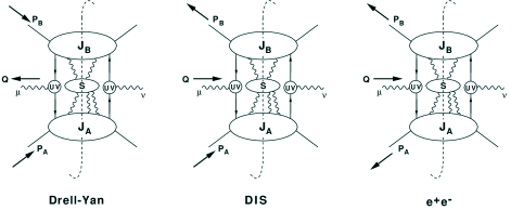
FIG. 7.: Dominant integration regions leading to the non-perturbative contributions to (a) Drell-Yan, (b) DIS, and (c) $e^{+}e^{-}$. These three processes are related via a crossing symmetry. $J_{A}$ and $J_{B}$ represent the jet subgraphs associated with the collinear partons from hadron $A(P_{A})$ and $B(P_{B})$, respectively. $S$ represents the subgraph of soft gluons and quarks which are connected to the rest of the process by soft gluons (but not soft quarks). The double-logarithms arise from $J_{A}$ and $J_{B}$.

The weak currents also contain $\gamma_{5}\gamma^{\mu}$ terms. This gives the possibility of another angular function in the small ${q_{T}}$ limit. With the same limiting hadronic structure, ${{P\kern-6.5pt\raise 2.0pt\hbox{/}}}_{\!\!A}\cdots{{P\kern-6.5pt\raise 2.0pt\hbox{/}}}_{\!\!B}$ we can have

$${\rm Tr}\{{{\ell\kern-4.6pt\raise 2.0pt\hbox{/}}}\gamma_{5}\gamma_{\mu}{{\ell\kern-4.6pt\raise 2.0pt\hbox{/}}}^{\prime}\gamma_{\nu}\}\ {\rm Tr}\{{{P\kern-6.5pt\raise 2.0pt\hbox{/}}}_{\!\!A}\gamma_{5}\gamma^{\mu}{{P\kern-6.5pt\raise 2.0pt\hbox{/}}}_{\!\!B}\gamma^{\nu}\},\\$$ (14)

which is proportional to the angular function ${\cal A}_{6}(\psi,\phi)=2\,{{\rm cosh}}(\psi)$ at ${q_{T}}=0$. (Note that both ${\cal A}_{1}(\psi,\phi)$ and ${\cal A}_{6}(\psi,\phi)$ are independent of the azimuthal angle $\phi$.) Thus $\Gamma_{6}$ has the structure

$$\Gamma_{6}(x,Q^{2},{q_{T}^{2}};j,j^{\prime}) = \Gamma_{6}^{Pert}(x,Q^{2},{q_{T}^{2}};j,j^{\prime})-\Gamma_{6}^{Asym}(x,Q^{2},{q_{T}^{2}};j,j^{\prime})+(-1)W(x,Q^{2},q_{T}^{2};j,j^{\prime}),$$ (15)

with the same function $W$ as in Eq. (LABEL:eq:smallqTdecompose). Again $W$ contains the terms that behave like $\log^{n}({q_{T}^{2}}/Q^{2})/{q_{T}^{2}}$ in perturbation theory, while $(\Gamma_{6}^{Pert}-\Gamma_{6}^{Asym})$ contain the less singular terms. Our object now will be to study the small ${q_{T}}$ function $W$.

B Parton Level Distributions

The above hadronic process takes place via the partonic sub-process $V(q)+a(k_{a})\to b(k_{b})+X$ where $V$ is an intermediate vector boson, and $a$ and $b$ denote parton species. The hadron structure function $W(x,Q^{2},{q_{T}^{2}};j,j^{\prime})$ is related to a perturbatively calculable parton level structure function $w_{a}({\widehat{x}},Q^{2},{q_{T}^{2}};j,j^{\prime})$ via

$$W(x,Q^{2},{q_{T}^{2}};j,j^{\prime}) = f_{a/A}\otimes w_{a}=\int_{x}^{1}{d\xi\over\xi}\ \sum_{a}f_{a/A}(\xi,\mu)\ w_{a}({\widehat{x}},Q^{2},{q_{T}^{2}};j,j^{\prime})\qquad,$$ (17)

with $\xi_{a}=k_{a}^{+}/P_{A}^{+}$ and ${\widehat{x}}=x/\xi_{a}$. Here $f_{a/A}$ is the  MS  parton distribution function. Note that the decay distribution function $d_{B/b}(\xi_{b},\mu)$ is absent since we have used the extra $\int z\,dz$ and the sum over hadrons from the definition of the energy distribution to integrate out the $d_{B/b}(\xi_{b},\mu)$ via the momentum sum rule,

$$\sum_{B}\ \int\ d\xi_{b}\ \xi_{b}\ d_{B/b}(\xi_{b},\mu) = 1\qquad.$$ (18)

The partonic structure function, $w_{a}({\widehat{x}},Q^{2},{q_{T}^{2}};j,j^{\prime})$, is obtained by first computing the partonic tensor

$$w^{\mu\nu}(k_{a},k_{b},q) = {\displaystyle{1\over 2}}\,\sum_{X,s,s^{\prime}}\ \int\ d^{4}x\ e^{-iq\cdot x}\ \langle k_{a},s|j^{\nu}(0)|k_{b},s^{\prime};X\rangle\ \langle k_{b},s^{\prime};X|j^{\mu}(0)|k_{a},s\rangle,$$ (19)

which is a matrix element of current operators. We then project out the appropriate angular component (cf., paper I), and extract the leading term in the ${q_{T}}\to 0$ limit. Explicit calculation will show that these limits (up to overall factors) are identical for the projection of the 1 and 6 tensors. In the small ${q_{T}}$ limit, the energy distribution function is then given by:

$${d\Sigma\over dx\ dQ^{2}\ d{q_{T}^{2}}\ d\phi} \simeq {\cal A}_{1}(\psi,\phi)\ \sum_{V_{1},V_{2}}\ \sum_{j,j^{\prime}}\ \Sigma_{0}(Q^{2};V_{1},V_{2},j,j^{\prime},1)\ \sum_{a}\ f_{a/A}(\xi,\mu)\otimes w_{a}({\widehat{x}},Q^{2},{q_{T}^{2}};j,j^{\prime})$$ (20)

$$- {\cal A}_{6}(\psi,\phi)\ \sum_{V_{1},V_{2}}\ \sum_{j,j^{\prime}}\ \Sigma_{0}(Q^{2};V_{1},V_{2},j,j^{\prime},6)\ \sum_{a}\ f_{a/A}(\xi,\mu)\otimes w_{a}({\widehat{x}},Q^{2},{q_{T}^{2}};j,j^{\prime})$$ (21)

$$+ {\rm\ plus\ terms\ less\ singular\ than\ 1/{q_{T}^{2}}}\qquad.$$ (22)

Again, the relative minus sign is simply due to the definition of ${\cal A}_{k}(\psi,\phi)$ and $\Sigma_{0}(Q^{2};V_{1},V_{2},j,j^{\prime},k)$.

C The Asymptotic Energy Distribution Functions

We observe (from the results of paper I) that the perturbative $\Gamma_{1}^{Pert}(x,Q^{2},q_{T}^{2};j,j^{\prime})$ and $\Gamma_{6}^{Pert}(x,Q^{2},q_{T}^{2};j,j^{\prime})$ diverge as $1/{q_{T}^{2}}$ for ${q_{T}}\to 0$. To identify the singular terms, we can expand the on-shell delta function for small ${q_{T}}$ using

$$\ 2\pi\ \delta\!\left[(q^{\mu}+k_{a}^{\mu}-k_{b}^{\mu})^{2}\right] = {2\pi{\widehat{x}}\over Q^{2}}\ \Biggl{\{}\ln\left({Q^{2}\over{q_{T}^{2}}}\right)\delta(1-{\widehat{x}})\ \delta(1-{\widehat{z}})+{\delta(1-{\widehat{z}})\over(1-{\widehat{x}})_{+}}+{\delta(1-{\widehat{x}})\over(1-{\widehat{z}})_{+}}\Biggr{\}},$$ (23)

where the “$+$”-prescriptions is defined as usual by:

$$\int_{z}^{1}dy\ {\displaystyle{G(y)\over(1-y)_{+}}} = G(1)\ln(1-z)+\int_{z}^{1}dy\ {\displaystyle{[G(y)-G(1)]\over(1-y)}}\qquad.$$ (25)

Taking the ${q_{T}}\to 0$ limit for the results of paper I, we find the partonic energy distribution to be

$$w_{a}^{Asym}({\widehat{x}},Q^{2},{q_{T}^{2}};j,j^{\prime}) = \left[{\displaystyle{16\pi^{2}\,\alpha_{s}\over{q_{T}^{2}}}}\right]\ \Biggl{\{}\delta_{a,j}\,\delta(1-{\widehat{x}})\ C_{F}\ \left[2\ln\left({\displaystyle{Q^{2}\over{q_{T}^{2}}}}\right)-3\right]$$ (26)

$$+ \delta_{a,j}\ C_{F}\ \left[{\displaystyle{1+{\widehat{x}}^{2}\over 1-{\widehat{x}}}}\right]_{+}\ +\delta_{a,g}\ \left[{\displaystyle{{\widehat{x}}^{2}+(1-{\widehat{x}})^{2}\over 2}}\right]\Biggl{\}}\qquad,$$ (27)

where we use $\delta_{a,j}$ and $\delta_{a,g}$ for the quark and gluon contributions, respectively. For convenience, we denote the asymptotic limit ${q_{T}}\to 0$ of $w_{a}$ by $w_{a}^{Asym}$.

In this limit, we can greatly simplify this expression by identifying the QCD splitting functions. We present the result for the hadronic structure function convoluted with the parton distributions, (cf., Eq. (17)):

$$\Gamma^{Asym}(x,Q^{2},{q_{T}^{2}};j,j^{\prime}) = \left[{\displaystyle{16\pi^{2}\,\alpha_{s}\over{q_{T}^{2}}}}\right]\ \Bigl{\{}f_{j/A}(x)\ C_{F}\ \left[2\ \ln\left({\displaystyle{Q^{2}\over{q_{T}^{2}}}}\right)-3\right]$$ (28)

$$+ f_{j/A}\otimes P_{q/q}+f_{g/A}\otimes P_{q/g}\Bigr{\}}\qquad,$$ (29)

where $\otimes$ represents a convolution in ${\widehat{x}}$. In the simple form above, it is easy to identify the separate contributions. The last two terms arise from the collinear singularities, and are proportional to the appropriate first order splitting kernel, $P_{q/q}$ and $P_{q/g}$. It is the remaining term in which we are interested as these arise from the soft gluon processes. We note that $\Gamma^{Asym}$ is defined such that the combination $\Gamma^{Pert}-\Gamma^{Asym}$ has only logarithmic singularities as ${q_{T}}\to 0$.

III Sudakov Form Factor

In this section, we display the structure of $d\Sigma/dx\,dQ^{2}\,dq_{T}^{2}\,d\phi$ with the Sudakov summation of logarithms. This provides the basis a formula that includes nonperturbative effects, developed in Sec. 6. In addition, in Sec. 4 we compare the summed form of this section with the order $\alpha_{s}$ form of $d\Sigma/dx\,dQ^{2}\,dq_{T}^{2}\,d\phi$ from Sec. 2, in order to extract the coefficients that appear in the summed form.

A Bessel Transform of $w_{a}({\widehat{x}},Q^{2},{q_{T}^{2}};j,j^{\prime})$

It proves convenient to introduce a Fourier transform between transverse momentum space (${q_{T}}$) and impact parameter space ($b$),

$$w_{a}({\widehat{x}},Q^{2},{q_{T}^{2}};j,j^{\prime}) = \int{d^{2}b\over(2\pi)^{2}}\ e^{i{q_{T}}\cdot b}\ \widetilde{w}_{a}({\widehat{x}},Q^{2},b^{2};j,j^{\prime})$$ (30)

$$= \int_{0}^{\infty}{db\over 2\pi}\ b\ J_{0}(b\,{q_{T}})\ \widetilde{w}_{a}({\widehat{x}},Q^{2},b^{2};j,j^{\prime})\qquad,$$ (31)

as $\widetilde{w}_{a}({\widehat{x}},Q^{2},b^{2};j,j^{\prime})$ will have a simple structure.${}^{\cite[cite]{[\@@bibref{Number}{CSS}{}{}]}}$ Effectively, we make use of the renormalization group equation to sum the logs of $Q^{2}$, and gauge invariance to sum the logs of ${q_{T}}\sim 1/b$. The Fourier transform also maps the ${q_{T}}$ singularities at the origin to the large $b$ behavior of $\widetilde{w}_{a}({\widehat{x}},Q^{2},b^{2};j,j^{\prime})$; we will take advantage of this when we consider non-perturbative contributions.

B Sudakov Form Factor

The structure function in impact parameter space $\widetilde{w}_{a}({\widehat{x}},Q^{2},b^{2};j,j^{\prime})$ has the factorized form:

$$\widetilde{w}_{a}({\widehat{x}},Q^{2},b^{2};j,j^{\prime}) = C^{IN}_{ja}\big{(}{\widehat{x}},b\mu\big{)}\ \sum_{a^{\prime}}\int\,d{\widehat{z}}\,{\widehat{z}}\ C^{OUT}_{a^{\prime}\,j^{\prime}}\big{(}{\widehat{z}},b\mu\big{)}\ e^{-S(b)}\qquad.$$ (32)

This form is from references [28] and [14] applied to the DIS process, and generalized to include vector bosons other than the photon. The last exponential factor is the Sudakov form factor:

$$S(b) = \int_{C_{1}^{2}/b^{2}}^{C_{2}^{2}Q^{2}}\ {d\mu^{2}\over\mu^{2}}\left\{\ln\left[{C_{2}^{2}Q^{2}\over\mu^{2}}\right]A(\alpha_{s}(\mu))+B(\alpha_{s}(\mu))\right\}\qquad.$$ (33)

The logarithm in the exponential is characteristic of the gauge theory. It arises from the soft gluon summation in QCD at the low transverse momentum ${q_{T}^{2}}\ll Q^{2}$. The arbitrary constants $\{C_{1},C_{2}\}$ reflect the freedom in the choice of renormalization scale. We choose $\{C_{1},C_{2}\}$ to be

$$C_{1} = 2e^{-\gamma_{E}}$$ (34)

$$C_{2} = 1\qquad.$$ (35)

The functions $A$, $B$ and the hard scattering functions $C$’s are simple power series in the strong coupling constant $\alpha_{s}$ with numerical coefficients:

$$A(\alpha_{s}(\mu)) = \sum_{N=1}^{\infty}\ \left\{{\alpha_{s}(\mu)\over(2)\pi}\right\}^{N}\ A_{N}$$ (36)

$$B(\alpha_{s}(\mu)) = \sum_{N=1}^{\infty}\ \left\{{\alpha_{s}(\mu)\over(2)\pi}\right\}^{N}\ B_{N}$$ (37)

$$C_{ja}^{IN}({\widehat{x}},b\mu) = \delta(1-{\widehat{x}})\,\delta_{ja}+\sum_{N=1}^{\infty}\ C_{ja}^{IN(N)}({\widehat{x}},b\mu)\ \left\{{\alpha_{s}(\mu)\over(2)\pi}\right\}^{N}$$ (38)

$$C_{a^{\prime}j^{\prime}}^{OUT}({\widehat{z}},b\mu) = \delta(1-{\widehat{z}})\,\delta_{a^{\prime}j^{\prime}}+\sum_{N=1}^{\infty}\ C_{a^{\prime}j^{\prime}}^{OUT(N)}({\widehat{z}},b\mu)\ \left\{{\alpha_{s}(\mu)\over(2)\pi}\right\}^{N}\qquad.$$ (39)

The normalization has been chosen such that each hard scattering function $C$ equals a $\delta$-function at leading order.

As noted in reference [14], in the limit $Q\to\infty$, all logarithms may be counted as being equally large. Therefore, to evaluate the cross section at ${q_{T}}\simeq 0$ to an approximation of “degree $N$,” one must evaluate $A$ to order ${\alpha_{s}}^{N+2}$, $B$ to order ${\alpha_{s}}^{N+1}$, $C^{IN}$ and $C^{OUT}$ to order ${\alpha_{s}}^{N}$, and the $\beta$ function order ${\alpha_{s}}^{N+2}$. In particular, an extra order in $A$ is necessary due to the extra logarithmic factor in Eq. (33). For the present calculation, we evaluate $A$ to order ${\alpha_{s}}^{2}$, $B$ to order ${\alpha_{s}}^{1}$, $C^{IN}$ and $C^{OUT}$ to order ${\alpha_{s}}^{1}$, and the $\beta$ function to order ${\alpha_{s}}^{2}$. This yields the cross section to order ${\alpha_{s}}^{1}$ for large ${q_{T}}$, to order ${\alpha_{s}}^{0}$ for small ${q_{T}}$, and the cross section integrated over ${q_{T}}$ to ${\alpha_{s}}^{1}$.

C Perturbative Expansion of the Sudakov Form Factor

We can extract the $A_{i}$ and $B_{i}$ coefficients of the Sudakov factor by expanding $\widetilde{w}_{a}({\widehat{x}},Q^{2},b^{2};j,j^{\prime})$ of Eq. (32) in ${\alpha_{s}}$, and comparing with the perturbative calculation of paper I. Here, we take a fixed momentum scale $\mu_{0}$ in $\alpha_{s}(\mu_{0})$ as the running of $\alpha_{s}(\mu)$ contributes only to higher orders. We can now compute the integral over $\mu^{2}$ analytically to obtain:

$$S(b) = \int_{C_{1}^{2}/b^{2}}^{C_{2}^{2}Q^{2}}\ {d\mu^{2}\over\mu^{2}}\ \left[\ln\left[{C_{2}^{2}Q^{2}\over\mu^{2}}\right]A(\alpha_{s}(\mu))+B(\alpha_{s}(\mu))\right]$$ (40)

$$\simeq {\alpha_{s}(\mu_{0})\over(2)\,\pi}\left[A_{1}\,{L^{2}\over 2}+B_{1}L\right]\qquad,$$ (41)

where

$$L = \ln\left[{C_{2}^{2}\over C_{1}^{2}}\ b^{2}\,Q^{2}\right]\qquad.$$ (42)

We expand the Sudakov exponential out to order ${\alpha_{s}}^{1}$,

$$e^{-S(b)} \simeq 1-S(b)+{\cal O}({\alpha_{s}}^{2})\qquad,$$ (43)

and perform the Bessel transform of $\widetilde{w}_{a}({\widehat{x}},Q^{2},b^{2};j,j^{\prime})$ (cf., Eq. (32)) to obtain the partonic structure function in momentum space:

$$w_{a}({\widehat{x}},Q^{2},{q_{T}^{2}};j,j^{\prime}) = \int_{0}^{\infty}{db\over 2\pi}\ b\ J_{0}(b\,{q_{T}})\ \left[\delta_{a,j}\,\delta(1-{\widehat{x}})+{\displaystyle{{\alpha_{s}}(\mu)\over(2)\pi}}\ C_{a,j}^{IN\,(1)}({\widehat{x}},b\mu)\right]$$ (44)

$$\times \sum_{a^{\prime}}\ \left[\delta_{a^{\prime},j^{\prime}}+\int_{0}^{1}\,{\widehat{z}}\,d{\widehat{z}}\ {\displaystyle{{\alpha_{s}}(\mu)\over(2)\pi}}\ C_{a^{\prime},j^{\prime}}^{OUT\,(1)}({\widehat{z}},b\mu)\right]$$ (45)

$$\times \left[1-S(b)+{\cal O}({\alpha_{s}}^{2})\right]\qquad,$$ (46)

where we have used the first order expressions for $C^{IN\,(N)}_{jk}({\widehat{x}},\mu b)$ and $C^{OUT\,(N)}_{jk}({\widehat{z}},\mu b)$.

Finally, we integrate to obtain the ${\cal O}({\alpha_{s}}^{1})$ terms for finite ${q_{T}}$:

$$w_{a}({\widehat{x}},Q^{2},{q_{T}^{2}};j,j^{\prime}) \simeq \left[{\displaystyle{16\pi^{2}\,\alpha_{s}\over{q_{T}^{2}}}}\right]\ \Biggl{\{}\delta_{a,j}\,\delta(1-{\widehat{x}})\ \left[{\displaystyle{2A_{1}\over(2)}}\,\left\{\ln\left({\displaystyle{Q^{2}\over{q_{T}^{2}}}}\right)-2\ln\left({\displaystyle{e^{\gamma_{E}}C_{1}\over 2C_{2}}}\right)\right\}+{\displaystyle{2B_{1}\over(2)}}\right]\,$$ (49)

$$\qquad\qquad\qquad+\ \delta_{a,j}\ P_{q/q}(x)+\ \delta_{a,g}\ P_{q/g}(x)$$

$$\qquad\qquad\qquad+{\rm\ terms\ proportional\ to\ }\delta({q_{T}^{2}})\Biggl{\}}\qquad.$$

Here, we have use the fact that the renormalization group equation tells us the form of $C^{IN(1)}({\widehat{x}},\mu b)$ and $C^{OUT(1)}({\widehat{z}},\mu b)$ must be a splitting kernel times $\log[\mu b]$, plus a function independent of $\mu$ and $b$. Equivalently, for the hadronic structure function, we find:

$$W(x,Q^{2},{q_{T}^{2}};j,j^{\prime}) \simeq \left[{\displaystyle{16\pi^{2}\,\alpha_{s}\over{q_{T}^{2}}}}\right]\ \Biggl{\{}f_{j/A}(x)\ \left[{\displaystyle{2A_{1}\over(2)}}\,\left\{\ln\left({\displaystyle{Q^{2}\over{q_{T}^{2}}}}\right)-2\ln\left({\displaystyle{e^{\gamma_{E}}C_{1}\over 2C_{2}}}\right)\right\}+{\displaystyle{2B_{1}\over(2)}}\right]\,$$ (52)

$$\qquad\qquad\qquad+\ f_{j/A}\otimes\ P_{q/q}+\ f_{g/A}\otimes\ P_{q/g}$$

$$\qquad\qquad\qquad+{\rm\ terms\ proportional\ to\ }\delta({q_{T}^{2}})\Biggl{\}}\qquad.$$

We will compare the first-order expansions in Eq. (49) and Eq. (52) with the asymptotic limit of the perturbative calculations of Sec. II to extract the desired $A_{1}$ and $B_{1}$ coefficients.

IV Comparing Asymptotic and Sudakov Contributions

In this section, we compare the summed form of $d\Sigma/dx\,dQ^{2}\,dq_{T}^{2}\,d\phi$ with the order $\alpha_{s}$ form, and thus extract the coefficients that appear in the summed form.

A Extraction of $A$ and $B$

Comparing the expansion of the Sudakov expression [Eq. (52)] with the asymptotic results [Eq. (29)], we obtain the order $\alpha_{s}^{1}$ coefficients $A_{1}$ and $B_{1}$,

$$A_{1} = (2)\ C_{F}$$ (53)

$$B_{1} = (2)\ 2\,C_{F}\,\ln\left[{C_{1}\over 2C_{2}}\,e^{\gamma_{E}-(3/4)}\right]\qquad.$$ (54)

With our particular choice of the arbitrary constants $\{C_{1},C_{2}\}$ in Eq. (35), we have:

$$A_{1} = (2)\ C_{F}$$ (55)

$$B_{1} = (2)\ \left[{\displaystyle{-3\over\phantom{-}2}}\right]\ C_{F}\qquad.$$ (56)

We find that the results for $A_{1}$ and $B_{1}$ obtained above are identical to those found in reference [28] for Drell-Yan production, as well as those found in reference [15] for $e^{+}\,e^{-}$ annihilation. This apparent crossing symmetry has been demonstrated at order $\alpha_{s}^{2}$ by Trentadue.${}^{\cite[cite]{[\@@bibref{Number}{trentadue}{}{}]}}$ In light of this result, we shall make use of the $A_{2}$ coefficient${}^{\cite[cite]{[\@@bibref{Number}{trentadue}{}{}]}}$

$$A_{2} = (4)\left\{{67\over 9}-{\pi^{2}\over 3}-{10\over 27}\,N_{f}+{2\over 9}(33-2N_{f})\ln\left({C_{1}\over 2\,e^{-\gamma_{E}}}\right)\right\}\qquad.$$ (57)

The extra order in the $A_{i}$ expansion will compensate extra logarithm $L$ which is not present for the $B_{i}$ terms.

B Expansion of $C^{IN}$ and $C^{OUT}$

$C^{IN}$ and $C^{OUT}$ terms are obtained by comparing the terms in the perturbative expansion proportional to $\delta({q_{T}})$ with the expanded summed form. Since the virtual graphs yield contributions only proportional to $\delta({q_{T}})$, they will only enter $C^{IN}$ and $C^{OUT}$. The real graphs yield both zero and finite ${q_{T}}$ terms; therefore, they will contribute to both $A_{i}$, $B_{i}$, and the $C^{IN}$ and $C^{OUT}$ coefficients. The calculation of the virtual graphs has been performed by Meng,${}^{\cite[cite]{[\@@bibref{Number}{meng}{}{}]}}$ and we make use of those results.

We have defined the $C({\widehat{x}},\mu b)$ coefficients such that at leading order, they are

$$C^{IN\,(0)}_{jk}({\widehat{x}},\mu b) = \delta_{jk}\,\delta(1-{\widehat{x}})$$ (58)

$$C^{OUT\,(0)}_{jk}({\widehat{z}},\mu b) = \delta_{jk}\,\delta(1-{\widehat{z}})$$ (59)

$$C^{IN\,(0)}_{jg}({\widehat{x}},\mu b) = C^{OUT\,(0)}_{gk}({\widehat{z}},\mu b)=0\qquad.$$ (60)

(Here, $j$ and $k$ denote quarks and anti-quarks, and $g$ denotes gluons.) At next to leading order, we find that $C^{IN\,(1)}({\widehat{x}},\mu b)$ match those calculated by CS for the Drell-Yan process:${}^{\cite[cite]{[\@@bibref{Number}{CS}{}{}]}}$

$$C^{IN\,(1)}_{jk}({\widehat{x}},\mu b) = \delta_{jk}\Biggl{\{}{2\over 3}(1-{\widehat{x}})+P_{q/q}({\widehat{x}})\ \ln\left({\lambda\over\mu b}\right)$$ (61)

$$+ \delta(1-{\widehat{x}})\ \Biggl{[}-C_{F}\,\ln^{2}\left({C_{1}\ e^{-3/4}\over C_{2}\,\lambda}\right)+{\pi^{2}\over 3}-{23\over 12}\Biggr{]}\Biggr{\}}$$ (62)

$$C^{IN\,(1)}_{jg}({\widehat{x}},\mu b) = {1\over 2}{\widehat{x}}(1-{\widehat{x}})+P_{j/g}({\widehat{x}})\ \ln\left({\lambda\over\mu b}\right)\qquad.$$ (63)

The $C^{OUT\,(1)}({\widehat{z}},\mu b)$ are simply those for $e^{+}e^{-}$ as given in reference [15]:

$$C^{OUT\,(1)}_{jk}({\widehat{z}},\mu b) = \delta_{jk}\Biggl{\{}{2\over 3}(1-{\widehat{z}})+P_{q/q}({\widehat{z}})\ \ln\left({\lambda\over\mu b}\right)$$ (64)

$$+ \delta(1-{\widehat{z}})\ \Biggl{[}-C_{F}\,\ln^{2}\left({C_{1}\ e^{-3/4}\over C_{2}\,\lambda}\right)+{\pi^{2}\over 3}-{29\over 12}\Biggr{]}\Biggr{\}}$$ (65)

$$C^{OUT\,(1)}_{gk}({\widehat{z}},\mu b) = {2\over 3}\,{\widehat{z}}+P_{g/k}({\widehat{z}})\ \ln\left({\lambda\over\mu b}\right)\qquad,$$ (66)

where we define $\lambda=2e^{-\gamma_{E}}$ to simplify the notation. Note that $C^{IN}$ and $C^{OUT}$ are only a function of the ratio $C_{1}/C_{2}$.

C Complete Expression

Now that we have obtained $A_{1}$, $A_{2}$, and $B_{1}$, we can substitute into equation Eq. (33) to obtain the complete Sudakov contribution (including the full $\alpha_{s}(\mu)$ dependence). We choose to perform the $\mu$ integral analytically, as the Bessel transform would be prohibitively CPU intensive if we did not. To facilitate this computation we provide an integral table in Appendix G including all the necessary terms We are now ready to combine the separate parts of the calculation.

V Matching

We now have computed the contributions to the energy distribution functions for the perturbative $\Gamma_{k}^{Pert}$ in paper I [Eq. (17)], the summed (or Sudakov) $W(x,Q^{2},q_{T}^{2};j,j^{\prime})$ in Eq. (52), and the asymptotic $\Gamma_{k}^{Asym}$ in Eq. (29). We can simply assemble these pieces to form the total structure functions via:

$$\Gamma_{1}(x,Q^{2},{q_{T}^{2}};j,j^{\prime}) = \Gamma_{1}^{Pert}(x,Q^{2},{q_{T}^{2}};j,j^{\prime})+\phantom{(-1)}W(x,Q^{2},q_{T}^{2};j,j^{\prime})-\Gamma_{1}^{Asym}(x,Q^{2},{q_{T}^{2}};j,j^{\prime})$$ (67)

$$\Gamma_{6}(x,Q^{2},{q_{T}^{2}};j,j^{\prime}) = \Gamma_{6}^{Pert}(x,Q^{2},{q_{T}^{2}};j,j^{\prime})+(-1)W(x,Q^{2},q_{T}^{2};j,j^{\prime})-\Gamma_{6}^{Asym}(x,Q^{2},{q_{T}^{2}};j,j^{\prime}).$$ (68)

Here, $\Gamma_{k}^{Pert}$ and $\Gamma_{k}^{Asym}$ are evaluated at order ${\alpha_{s}}^{1}$, while $W$ contains a summation of perturbation theory. In the limit ${q_{T}}\to 0$, $\Gamma_{k}^{Pert}$ and $\Gamma_{k}^{Asym}$ will cancel each other leaving $W$ as we desire. In the limit ${q_{T}}\simeq Q$, $W$ and $\Gamma_{k}^{Asym}$ will cancel to leading order in $\alpha_{s}$; however, the finite difference may not be negligible. To ensure that we recover the proper result ($\Gamma_{k}^{Pert}$) for large ${q_{T}}$, we define the total energy distribution function ($\Gamma_{k}$) to be:

$$\Gamma_{1}(x,Q^{2},{q_{T}^{2}};j,j^{\prime}) = \Gamma_{1}^{Pert}(x,Q^{2},{q_{T}^{2}};j,j^{\prime})$$ (70)

$$+ {\cal T}\left({\displaystyle{{q_{T}}\over Q}}\right)\left\{\phantom{(-1)}W(x,Q^{2},q_{T}^{2};j,j^{\prime})-\Gamma_{1}^{Asym}(x,Q^{2},{q_{T}^{2}};j,j^{\prime})\right\}$$ (71)

$$\Gamma_{6}(x,Q^{2},{q_{T}^{2}};j,j^{\prime}) = \Gamma_{6}^{Pert}(x,Q^{2},{q_{T}^{2}};j,j^{\prime})$$ (72)

$$+ {\cal T}\left({\displaystyle{{q_{T}}\over Q}}\right)\left\{(-1)W(x,Q^{2},q_{T}^{2};j,j^{\prime})-\Gamma_{6}^{Asym}(x,Q^{2},{q_{T}^{2}};j,j^{\prime})\right\}\qquad,$$ (73)

where we introduce the arbitrary function

$${\cal T}\left({{q_{T}}\over Q}\right) = {1\over 1+\left(\rho\,{\displaystyle{{q_{T}}\over Q}}\right)^{4}}\qquad.$$ (75)

The transition function ${\cal T}({q_{T}}/Q)$ serves to switch smoothly from the matched formulas to the perturbative formula, and $\rho$ is an arbitrary parameter which determines the details of the matching. Fig. 8 displays ${\cal T}({q_{T}}/Q)$ for a range of $\rho$ values. We will choose $\rho=5$ which ensures that $\Gamma_{k}\simeq\Gamma_{k}^{Pert}$ for ${q_{T}}/Q\,{\lower 2.15277pt\hbox{$\stackrel{{\scriptstyle>}}{{\sim}}$}}\,0.4$, a conservative value.

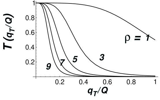
FIG. 8.: The matching function ${\cal T}({q_{T}}/Q)$ vs. $({q_{T}}/Q)$ for $\rho=\{1,3,5,7,9\}$. $\rho=1$ is the top curve, and $\rho=9$ is the bottom curve.

VI Non-Perturbative Contributions

In analogy with Eq. (17) and Eq. (32), the Bessel transform of the hadronic structure function is defined as:

$$W(x,Q^{2},q_{T}^{2};j,j^{\prime}) = \int\,{d^{2}b\over(2\pi)^{2}}\ e^{i{q_{T}}\cdot b}\ \widetilde{W}(x,Q^{2},b^{2};j,j^{\prime})\qquad.$$ (76)

When $b$ is small, we have:

$$\widetilde{W}(x,Q^{2},b^{2};j,j^{\prime}) = \int_{x}^{1}{\displaystyle{d\xi\over\xi}}\ \sum_{a}\ f_{a/A}(\xi,\mu)\ C^{IN}_{ja}\big{(}{\widehat{x}},b\mu\big{)}\ \sum_{a^{\prime}}\int\,d{\widehat{z}}\,{\widehat{z}}\ C^{OUT}_{a^{\prime}\,j^{\prime}}\big{(}{\widehat{z}},b\mu\big{)}\ e^{-S(b)}.$$ (77)

The perturbative calculation of $\widetilde{W}(x,Q^{2},b^{2};j,j^{\prime})$ is not reliable for $b{\lower 2.15277pt\hbox{$\stackrel{{\scriptstyle>}}{{\sim}}$}}1/\Lambda$. However, the integration over $b$ in Eq. (76) runs to infinitely large $b^{2}$, and the region $b{\lower 2.15277pt\hbox{$\stackrel{{\scriptstyle>}}{{\sim}}$}}1/\Lambda$ is important for values of $Q^{2}$ and ${q_{T}^{2}}$ of practical interest. In order to deal with the large $b^{2}$ region, we follow the method introduced in Refs. [28, 14]. We define a value $b_{\rm max}$ such that we can consider perturbation theory to be reliable for $b<b_{\rm max}$. (In our numerical examples, we take $1/b_{\rm max}=2\,{{\rm GeV}}$.) Then we define a function $b_{*}$ of $b$ such that $b_{*}\approx b$ for small $b$ and $b_{*}<b_{\rm max}$ for all $b$:

$$b_{*}={b\over\sqrt{1+b^{2}/b_{\rm max}^{2}}}\qquad.$$ (78)

We define a version of $\widetilde{W}(x,Q^{2},b^{2};j,j^{\prime})$ for which perturbation theory is always reliable by $\widetilde{W}(x,Q^{2},b_{*}^{2};j,j^{\prime})$. Note that for small $b$, the difference between $\widetilde{W}(b_{*})$ and $\widetilde{W}(b)$ is negligible because $b_{*}\approx b$. Conversely, perturbation theory is always applicable for the calculation of $\widetilde{W}(b_{*})$ because $b_{*}$ is small even when $b$ is large.

Next, we define a nonperturbative function $\exp(-S_{\rm NP}(b))$ as the ratio of $\widetilde{W}(b)$ and $\widetilde{W}(b_{*})$:

$$\widetilde{W}(x,Q^{2},b^{2};j,j^{\prime})=\widetilde{W}(x,Q^{2},b_{*}^{2};j,j^{\prime})\ e^{-S_{\rm NP}(x,Q^{2},b^{2};j,j^{\prime})}\qquad.$$ (79)

Ultimately, we will have to use nonperturbative information to determine $S_{\rm NP}(b)$. However, some important information is available to us. From Eq. (77), we see that

$${\displaystyle{\partial\log[\widetilde{W}(x,Q^{2},b^{2};j,j^{\prime})]\over\partial\log Q^{2}}}$$ (80)

is independent of $x,j,j^{\prime}$ and $Q^{2}$. This result is derived in perturbation theory, but at arbitrary order, so we presume that it holds even beyond perturbation theory. Then

$${\displaystyle{\partial S_{\rm NP}(x,Q^{2},b^{2};j,j^{\prime})\over\partial\log Q^{2}}}$$ (81)

is also independent of $x,j,j^{\prime},k$ and $Q^{2}$. That is, $S_{\rm NP}$ has the form

$$S_{\rm NP}(x,Q^{2},b^{2};j,j^{\prime})=\log\left(Q^{2}/Q_{0}^{2}\right)g_{1}(b)+\Delta S_{\rm NP}(x,b^{2};j,j^{\prime})\qquad.$$ (82)

(Here $Q_{0}$ is an arbitrary constant with dimensions of mass, inserted to keep the argument of the logarithm dimensionless.) Furthermore, in $\widetilde{W}$, the $x$ and $j$ dependence occurs in a separate factor from the $j^{\prime}$ dependence. Thus the second term in Eq. (82) above can be simplified to

$$S_{\rm NP}(x,Q^{2},b^{2};j,j^{\prime})=\log\left(Q^{2}/Q_{0}^{2}\right)g_{1}(b)+g_{A}(x,b^{2};j)+g_{B}(b^{2};j^{\prime})\qquad.$$ (83)

(Recall, we have integrated over ${\widehat{z}}$.)

Perturbation theory is not applicable for the calculation of the functions $g_{1}(b)$, $g_{A}(x,b^{2};j)$ and $g_{B}(b^{2};j^{\prime})$ for large $b$. For small $b$, perturbation theory tells us only that these functions approach 0 as $b\to 0$. This follows from Eq. (79), and the fact that $b_{*}/b\to 0$ when $b\to 0$. (See Ref. [14] for further discussion.) Since we learn little from perturbation theory, we turn to non-perturbative sources of information. Fortunately, the analogous functions in $e^{+}e^{-}$ annihilation and in the Drell-Yan process have been fit using experimental results.${}^{\cite[cite]{[\@@bibref{Number}{CS,DWS,yuanladinsky}{}{}]}}$

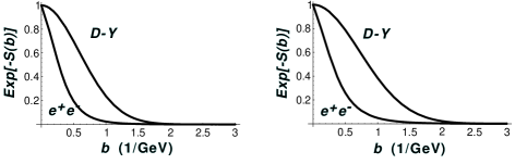
FIG. 9.: Comparison of the non-perturbative function $e^{-S_{NP}(b)}$ vs. $b$ for the Drell-Yan (Davies, Webber, and Stirling[17]) [upper line], and $e^{+}e^{-}$ (Collins and Soper[28]) [lower line], for $Q=30\,{{\rm GeV}}$ [Fig. (a)], and $Q=100\,{{\rm GeV}}$ [Fig. (b)].

We therefore ask whether the functions $g_{1}(b)$, $g_{A}(x,b^{2};j)$ and $g_{B}(b^{2};j^{\prime})$ in deeply inelastic scattering are related to the analogous functions in the other two processes. Consider first $g_{1}(b)$, the coefficient of $\log(Q^{2}/Q_{0}^{2})$. According to the analysis of Ref. [28], this function receives contributions from the two jet subdiagrams in Fig. 7(b). (In this figure, we use a space-like axial gauge.) The soft gluon connections in Fig. 7(b) affect $g_{A}(x,b^{2};j)$ and $g_{B}(b^{2};j^{\prime})$, but do not contribute “double logarithms,” and thus do not affect $g_{1}(b)$. Thus

$$g_{1}(b)\equiv g_{1}^{DIS}(b)=g_{1}^{\rm IN}(b)+g_{1}^{\rm OUT}(b)\qquad,$$ (84)

where $g_{1}^{\rm IN}(b)$ is associated with the incoming beam jet (the lower subdiagram in Fig. 7(b)) while $g_{1}^{\rm OUT}(b)$ is associated with the outgoing struck-quark jet (the upper subdiagram in Fig. 7(b)). In the Drell-Yan process, depicted in Fig. 7(a), there are two incoming beam jets and one has

$$g_{1}^{\rm DY}(b)=2g_{1}^{\rm IN}(b)\qquad.$$ (85)

In $e^{+}e^{-}$ annihilation, depicted in Fig. 7(c), there are two outgoing quark jets and one has

$$g_{1}^{e\bar{e}}(b)=2g_{1}^{\rm OUT}(b)\qquad.$$ (86)

Thus

$$g_{1}(b)\equiv g_{1}^{DIS}(b)=(1/2)\,g_{1}^{\rm DY}(b)+(1/2)\,g_{1}^{e\bar{e}}(b)\qquad.$$ (87)

In the following section, we show numerical results using Ref. [28] for $g_{1}^{e\bar{e}}(b)$ and Ref. [17] for $g_{1}^{\rm DY}(b)$.

The situation for $g_{A}(x,b^{2};j)$ and $g_{B}(b^{2};j^{\prime})$ is not so simple. Let us write

$$S_{\rm NP}^{\rm DY}(x,Q^{2},b^{2};j,j^{\prime})=\log\left(Q^{2}/Q_{0}^{2}\right)g_{1}^{\rm DY}(b)+g_{2}^{\rm DY}(x_{A},b^{2};j)+g_{2}^{\rm DY}(x_{B},b^{2};j^{\prime})\qquad.$$ (88)

for the Drell-Yan process and

$$S_{\rm NP}^{\bar{e}e}(x,Q^{2},b^{2};j,j^{\prime})=\log\left(Q^{2}/Q_{0}^{2}\right)g_{1}^{\bar{e}e}(b)+g_{2}^{\bar{e}e}(b^{2};j)+g_{2}^{\bar{e}e}(b^{2};j^{\prime})\qquad.$$ (89)

for the energy-energy correlation function in $e^{+}e^{-}$ annihilation. (Cf., Fig. 9.) One might like to assume that $g_{A}(x,b^{2};j)$ is the same function as $g_{2}^{\rm DY}(x,b^{2};j)$ while $g_{B}(b^{2};j^{\prime})$ is the same function as $g_{2}^{\bar{e}e}(b^{2};j^{\prime})$. However, this may not be true because all of these functions get contributions from the soft gluon exchanges that link the two jets in Fig. 7, (represented by the function $U(b)$ in Ref. [28]). Furthermore, the dependence of the functions $g_{2}^{\rm DY}(x,b^{2};j)$ and $g_{2}^{\bar{e}e}(b^{2};j^{\prime})$ on the flavors $j$ and $j^{\prime}$ has not been determined from experimental data. What we know are flavor averaged functions $g_{2}^{\rm DY}(x,b^{2})$ and $g_{2}^{\bar{e}e}(b^{2})$. Thus the best we can do is propose a model for the functions we need:

$$g_{A}(x,b^{2};j)+g_{B}(b^{2};j^{\prime})=t\,g_{2}^{\rm DY}(x,b^{2})+(1-t)\,g_{2}^{\bar{e}e}(b^{2})\qquad,$$ (90)

where $0<t<1$, with $g_{2}^{\bar{e}e}(b^{2})$ taken from Ref. [28] and $g_{2}^{\rm DY}(x,b^{2})$ taken from Ref. [17]. We vary the parameter $t$ between 0 and 1 to get an estimate of the uncertainty involved. (Cf., Fig. 10.)

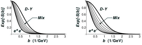
FIG. 10.: Interpolation of the non-perturbative function $e^{-S_{NP}(b)}$ vs. $b$ as a function of the $t$-parameter, $\{t=0,1/4,1/2,3/4,1\}$, for $Q=30\,{{\rm GeV}}$ [Fig. (a)], and $Q=100\,{{\rm GeV}}$ [Fig. (b)]. Note the variation of $e^{-S_{NP}(b)}$ as $t$ ranges over $[0,1]$ is narrower than the full range between the Drell-Yan and $e^{+}e^{-}$ case, (cf., Sec. VI).

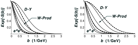
FIG. 11.: Comparison of the non-perturbative function $e^{-S_{NP}(b)}$ vs. $b$ for the case of Drell-Yan (Davies, Webber, and Stirling[17]) [upper dashed line], $e^{+}e^{-}$ (Collins and Soper[28]) [lower dashed line], and $W$-production (Ladinsky and Yuan[26]) [5 solid lines]. Fig. (a) is for $Q=10\,{{\rm GeV}}$ (left), and Fig. (b) is for $Q=100\,{{\rm GeV}}$ (right). The fits to $W$-production include an extra parameter $\tau=\hat{s}/s$; we allow $\tau$ to range over the values $\tau=\{10^{-3},10^{-2.75},10^{-2.5},10^{-2.25},10^{-2.0}\}$ where $\tau=10^{-2}$ is the upper curve, and $\tau=10^{-3}$ is the lower curve in $b$-space.

For comparison, we present the above parameterizations for the non-perturbative contributions with the recent fit by Ladinsky and Yuan${}^{\cite[cite]{[\@@bibref{Number}{yuanladinsky}{}{}]}}$ for W-production in Fig. 11. Ladinsky and Yuan introduce an extra degree of freedom by allowing for a $\tau=x_{A}\,x_{B}$ dependence. We present the comparison for a range of $\tau$; this allows one to gauge the effects of different non-perturbative estimates, and correlate the Ladinsky and Yuan parameterization with that presented in Eq. (82) and Eq. (90).

VII Reprise

For the benefit of the reader, we review the principal steps in the calculation of the energy distribution. The energy distribution is given by:

$${d\Sigma\over dx\,dQ^{2}\,d{q_{T}^{2}}\,d\phi} = \sum_{k=1}^{9}\ {d\Sigma_{k}\over dx\,dQ^{2}\,d{q_{T}^{2}}\,d\phi}$$ (91)

$$= \sum_{k=1}^{9}\ {\cal A}_{k}(\psi,\phi)\sum_{V_{1},V_{2}}\ \sum_{j,j^{\prime}}\ \Sigma_{0}(Q^{2};V_{1},V_{2},j,j^{\prime},k)\ \Gamma_{k}(x,Q^{2},q_{T}^{2};j,j^{\prime})\qquad,$$ (92)

where ${\cal A}_{k}(\psi,\phi)$ are the nine angular functions arising from hyperbolic $D^{1}(\psi,\phi)$ rotation matrices. The sum on $V_{1}$ and $V_{2}$ runs over vector boson types, $\{\gamma,Z\}$ or $\{W^{\pm}\}$ as appropriate. The sums over $j$ and $j^{\prime}$ include all quark flavors, $\{u,\bar{u},d,\bar{d},\dots\}$; for neutral currents, this sum is diagonal $(j=j^{\prime})$. The function $\Sigma_{0}(Q^{2};V_{1},V_{2},j,j^{\prime},k)$ includes factors for the coupling of the electron to the vector bosons as well as factors for the propagation of the vector bosons. The energy distribution function that we have computed is $\Gamma_{k}(x,Q^{2},q_{T}^{2};j,j^{\prime})$.

In the limit ${q_{T}}\to 0$, the $\Gamma_{1}$ and $\Gamma_{6}$ will contain the dominant singularities as their angular structure is proportional to the Born process. We define:

$$\Gamma_{1}(x,Q^{2},{q_{T}^{2}};j,j^{\prime}) = \Gamma_{1}^{Pert}(x,Q^{2},{q_{T}^{2}};j,j^{\prime})$$ (93)

$$+ {\cal T}\left({\displaystyle{{q_{T}}\over Q}}\right)\left\{\phantom{(-1)}W(x,Q^{2},q_{T}^{2};j,j^{\prime})-\Gamma_{1}^{Asym}(x,Q^{2},{q_{T}^{2}};j,j^{\prime})\right\}$$ (94)

$$\Gamma_{6}(x,Q^{2},{q_{T}^{2}};j,j^{\prime}) = \Gamma_{6}^{Pert}(x,Q^{2},{q_{T}^{2}};j,j^{\prime})$$ (95)

$$+ {\cal T}\left({\displaystyle{{q_{T}}\over Q}}\right)\left\{(-1)W(x,Q^{2},q_{T}^{2};j,j^{\prime})-\Gamma_{6}^{Asym}(x,Q^{2},{q_{T}^{2}};j,j^{\prime})\right\}$$ (96)

where the matching function ${\cal T}({q_{T}}/Q)$ [Eq. (75)] is provided to ensure proper behavior as ${q_{T}}\to Q$. $\Gamma_{k}^{Pert}$ represents the perturbative results of paper I [Eq. (17)] calculated at order ${\alpha_{s}}^{1}$, $\Gamma_{k}^{Asym}$ represents the asymptotic limit (${q_{T}}\to 0$) of $\Gamma_{k}^{Pert}$ [Eq. (29)], and $W(x,Q^{2},q_{T}^{2};j,j^{\prime})$ represents the summed (Sudakov) term [Eq. (32)] which is finite as ${q_{T}}\to 0$. Note the function $W(x,Q^{2},q_{T}^{2};j,j^{\prime})$ the same for both $\Gamma_{1}$ and $\Gamma_{6}$.

The form of the Sudakov structure function is particularly simple in impact parameter space:

$$W(x,Q^{2},q_{T}^{2};j,j^{\prime}) = \int\,{d^{2}b\over(2\pi)^{2}}\ e^{i{q_{T}}\cdot b}\ \widetilde{W}(x,Q^{2},b^{2};j,j^{\prime})\qquad.$$ (97)

To ensure that the calculation is reliable for large $b$ (small ${q_{T}}$), we introduce:

$$\widetilde{W}(x,Q^{2},b^{2};j,j^{\prime})=\widetilde{W}(x,Q^{2},b_{*}^{2};j,j^{\prime})\ e^{-S_{\rm NP}(x,Q^{2},b^{2};j,j^{\prime})}\qquad,$$ (98)

where $b_{*}\in[0,b_{max}]$ for $b\in[0,\infty]$.

The perturbative function $\widetilde{W}(x,Q^{2},b_{*}^{2};j,j^{\prime})$ is given by:

$$\widetilde{W}(x,Q^{2},b_{*}^{2};j,j^{\prime}) = \int_{x}^{1}{\displaystyle{d\xi\over\xi}}\ \sum_{a}\ f_{a/A}(\xi,\mu)\ C^{IN}_{ja}\big{(}{\widehat{x}},b_{*}\mu\big{)}\ \int\,d{\widehat{z}}\,{\widehat{z}}\ \sum_{a^{\prime}}\ C^{OUT}_{a^{\prime}\,j^{\prime}}\big{(}{\widehat{z}},b_{*}\mu\big{)}\ e^{-S(b_{*})},$$ (99)

where ${\widehat{x}}=x/\xi$. For the incoming particles, there is an integration over a parton momentum fraction $\xi$, a sum over parton types $a=g,u,\bar{u},d,\bar{d},\dots$, a parton distribution function $f_{a/A}$ and a set of perturbative coefficients $C^{\rm IN}$. For the outgoing partons, there is an integration over parton momentum fraction $\hat{z}$, weighted by $\hat{z}$, a sum over parton types $a^{\prime}=g,u,\bar{u},d,\bar{d},\dots$, and there are perturbative coefficients $C^{\rm OUT}$ associated with the outgoing states. The heart of the formula is the Sudakov factor $\exp[-S(b_{*})]$, defined as:

$$S(b_{*}) = \int_{C_{1}^{2}/b_{*}^{2}}^{C_{2}^{2}Q^{2}}\ {d\mu^{2}\over\mu^{2}}\left\{\ln\left[{C_{2}^{2}Q^{2}\over\mu^{2}}\right]A(\alpha_{s}(\mu))+B(\alpha_{s}(\mu))\right\}\qquad.$$ (101)

The functions $A$, $B$, as well as $C^{\rm IN}$ and $C^{\rm OUT}$, have perturbative expansions in powers of $\alpha_{s}$. We choose the arbitrary constants $\{C_{1},C_{2}\}$ as in Eq. (35).

The non-perturbative contribution is parameterized in terms of the fits to $e^{+}e^{-}$ and Drell-Yan data.${}^{\cite[cite]{[\@@bibref{Number}{eedata,CS,DWS}{}{}]}}$

$$S_{\rm NP}(x,Q^{2},b^{2};j,j^{\prime})=\log\left[{\displaystyle{Q^{2}\over Q_{0}^{2}}}\right]\left\{{\displaystyle{g_{1}^{\rm DY}(b)+g_{1}^{e\bar{e}}(b)\over 2}}\right\}+t\ g_{2}^{\rm DY}(x,b^{2})+(1-t)\ g_{2}^{\bar{e}e}(b^{2})\qquad.$$ (102)

The arbitrary parameter $t\in[0,1]$ interpolates between the $e^{+}e^{-}$ and Drell-Yan form.

VIII Results

We present numerical results of the energy distribution function for representative values of $\{x,Q^{2}\}$ using the CTEQ3 parton distributions.${}^{\cite[cite]{[\@@bibref{Number}{cteq3}{}{}]}}$ We present results only for the $\Gamma_{1}$ set of structure functions, as the $\Gamma_{6}$ set have the identical ${q_{T}}\to 0$ structure (up to a sign). Recall that the structure functions are given by:

$$\Gamma_{1}(x,Q^{2},{q_{T}^{2}};j,j^{\prime}) = \Gamma_{1}^{Pert}(x,Q^{2},{q_{T}^{2}};j,j^{\prime})$$ (103)

$$+ {\cal T}\left({\displaystyle{{q_{T}}\over Q}}\right)\left\{W(x,Q^{2},q_{T}^{2};j,j^{\prime})-\Gamma_{1}^{Asym}(x,Q^{2},{q_{T}^{2}};j,j^{\prime})\right\}\qquad.$$ (104)

Making use of Eq. (7), we have a parallel relation for the energy distribution function:

$${\displaystyle{d\Sigma_{1}(x,Q^{2},{q_{T}^{2}};j,j^{\prime})\over dx\,dQ^{2}\,d{q_{T}^{2}}\,d\phi}} = {\displaystyle{d\Sigma_{1}^{Pert}(x,Q^{2},{q_{T}^{2}};j,j^{\prime})\over dx\,dQ^{2}\,d{q_{T}^{2}}\,d\phi}}$$ (105)

$$+ {\cal T}\left({\displaystyle{{q_{T}}\over Q}}\right)\left\{{\displaystyle{d\Sigma_{1}^{Sum}(x,Q^{2},{q_{T}^{2}};j,j^{\prime})\over dx\,dQ^{2}\,d{q_{T}^{2}}\,d\phi}}-{\displaystyle{d\Sigma_{1}^{Asym}(x,Q^{2},{q_{T}^{2}};j,j^{\prime})\over dx\,dQ^{2}\,d{q_{T}^{2}}\,d\phi}}\right\},$$ (106)

where we use the “Sum” superscript to denote the summed Sudakov contribution derived from $W$. We will examine both the individual terms as well as the total in the following. We will use the shorthand $d\Sigma_{1}\equiv d\Sigma_{1}(x,Q^{2},{q_{T}^{2}};j,j^{\prime})/(dx\,dQ^{2}\,d{q_{T}^{2}}\,d\phi)$

A ${q_{T}}$ Distributions

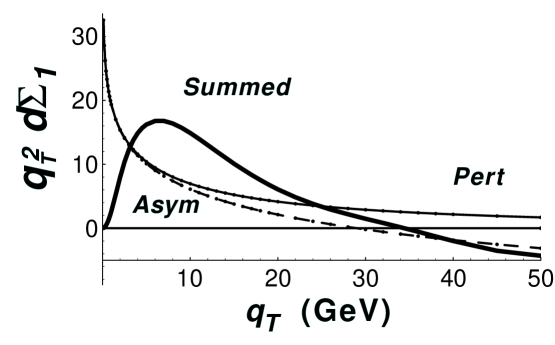
FIG. 12.: The contributions to the energy distribution function ${q_{T}^{2}}\,d\Sigma_{1}/(dx\,dQ^{2}\,d{q_{T}^{2}}\,d\phi)$ as a function of ${q_{T}}$, for $Q=100\,{{\rm GeV}}$, $x=0.3$. (Recall, $d\Sigma_{1}$ and $d\Sigma_{6}$ are independent of $\phi$.) Perturbative (thin), asymptotic (dashed), and summed (thick). Note how the perturbative and asymptotic cancel as ${q_{T}}\rightarrow 0$. For ${q_{T}}\rightarrow Q$, the asymptotic and summed cancel to leading order only. (A zero reference line is indicated.) $d\Sigma_{1}$ is in units of ${{\rm GeV}}^{-5}$, and is multiplied by $10^{9}$ for clarity of the plot.

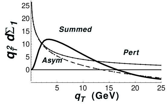
FIG. 13.: The contributions to the energy distribution function ${q_{T}^{2}}\,d\Sigma_{1}/(dx\,dQ^{2}\,d{q_{T}^{2}}\,d\phi)$ as a function of ${q_{T}}$, for $Q=30\,{{\rm GeV}}$, $x=0.1$. (Recall, $d\Sigma_{1}$ and $d\Sigma_{6}$ are independent of $\phi$.) Perturbative (thin), asymptotic (dashed), and summed (thick). Note how the perturbative and asymptotic cancel as ${q_{T}}\rightarrow 0$. For ${q_{T}}\rightarrow Q$, the asymptotic and summed cancel to leading order only. (A zero reference line is indicated.) $d\Sigma_{1}$ is in units of ${{\rm GeV}}^{-5}$, and is multiplied by $10^{6}$ for clarity of the plot.

In Fig. 12 and Fig. 13, we show the separate contributions to $d\Sigma_{1}$ as a function of ${q_{T}}$ for two choices of $\{x,Q^{2}\}$. We have included an extra factor of ${q_{T}^{2}}$ to make the features of the plot more legible. As anticipated, we see that $d\Sigma_{1}^{Pert}\simeq d\Sigma_{1}^{Asym}$ as ${q_{T}}\to 0$ leaving $d\Sigma_{1}\simeq d\Sigma_{1}^{Sum}$. For large ${q_{T}}$, we find $d\Sigma_{1}^{Sum}-d\Sigma_{1}^{Asym}\simeq 0$, but this cancellation is not as precise as the above because the relation $\Gamma^{Sum}-\Gamma^{Asym}\simeq 0$ holds only to first-order. Therefore, in the following figures we shall include the ${\cal T}({q_{T}^{2}}/Q^{2})$ factor to ensure that $d\Sigma_{1}^{Sum}-d\Sigma_{1}^{Asym}$ is smoothly turned off at large ${q_{T}}$. The fact that $d\Sigma_{1}^{Sum}$ and $d\Sigma_{1}^{Asym}$ become negative for large ${q_{T}}$ reminds us that these expressions were approximations valid only for ${q_{T}}\ll Q$.

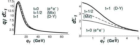
FIG. 14.: The total contribution to the energy distribution function $d\Sigma_{1}/(dx\,dQ^{2}\,d{q_{T}^{2}}\,d\phi)$ as a function of ${q_{T}}$ for different choices of the non-perturbative function, $S_{NP}(b)$, for $Q=100\,{{\rm GeV}}$, $x=0.3$. Fig. (a) has an extra factor of ${q_{T}^{2}}$ to make the plot more legible. Fig. (b) demonstrates that the summed contribution has a finite limit as ${q_{T}}\to 0$. We vary the $t$-parameter from $t=1$ (thick) corresponding to the Drell-Yan case, to $t=1/2$ (dashed) corresponding to the mixed case, to $t=0$ (thin) corresponding to the $e^{+}e^{-}$ case. For ${q_{T}}\rightarrow Q$, we use the function ${\cal T}({q_{T}}/Q)$ with $\rho=5$ to smoothly switch between large and small ${q_{T}}$. $d\Sigma_{1}$ is in units of ${{\rm GeV}}^{-5}$, and is multiplied by $10^{9}$ for clarity of the plot.

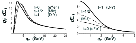
FIG. 15.: The total contribution to the energy distribution function $d\Sigma_{1}/(dx\,dQ^{2}\,d{q_{T}^{2}}\,d\phi)$ as a function of ${q_{T}}$ (scaled by $10^{9}$), for different choices of the non-perturbative function, $S_{NP}(b)$, for $Q=30\,{{\rm GeV}}$, $x=0.1$. Fig. (a) has an extra factor of ${q_{T}^{2}}$ to make the plot more legible. Fig. (b) demonstrates that the summed contribution has a finite limit as ${q_{T}}\to 0$. We vary the $t$-parameter from $t=1$ (thick) corresponding to the Drell-Yan case, to $t=1/2$ (dashed) corresponding to the mixed case, to $t=0$ (thin) corresponding to the $e^{+}e^{-}$ case. For ${q_{T}}\rightarrow Q$, we use the function ${\cal T}({q_{T}}/Q)$ with $\rho=5$ to smoothly switch between large and small ${q_{T}}$. $d\Sigma_{1}$ is in units of ${{\rm GeV}}^{-5}$, and is multiplied by $10^{6}$ for clarity of the plot.

Having examined the separate terms, we now turn our attention to the energy distribution function, $d\Sigma_{1}$. Again, we have included an extra factor of ${q_{T}^{2}}$ in Fig. 14(a) and Fig. 15(a) to make the features of the plot more legible. In Fig. 14(b) and Fig. 15(b), we plot $d\Sigma_{1}$ in the small ${q_{T}}$ region (without an extra ${q_{T}^{2}}$ factor) to demonstrate that the summed results approach a finite limit as ${q_{T}}\to 0$. We present the results for three choices of the non-perturbative function $S_{\rm NP}(x,Q^{2},b^{2};j,j^{\prime})$ as parameterized in Eq. (90). The choice $t=0$ corresponds to the $e^{+}e^{-}$ limit,${}^{\cite[cite]{[\@@bibref{Number}{CS}{}{}]}}$ while $t=1$ corresponds to the Drell-Yan limit,${}^{\cite[cite]{[\@@bibref{Number}{DWS}{}{}]}}$ and $t=1/2$ corresponds to an even mix of the above. The difference due to the non-perturbative contribution is quite significant for low ${q_{T}}$. The $t=0$ ($e^{+}e^{-}$) non-perturbative function, which is much narrower in $b$-space, yields a broader energy distribution; this is clearly evident in the figures as we see the peak move to lower ${q_{T}}$ values as we shift from the $t=0$ ($e^{+}e^{-}$) to $t=1$ (Drell-Yan). At large ${q_{T}}$, $d\Sigma_{1}$ is independent of the non-perturbative contributions, since it is dominated by $d\Sigma_{1}^{Pert}$.

Clearly, the HERA data should be able to distinguish between this range of distributions, particularly in the small ${q_{T}}$ regime where the span of the non-perturbative contributions are significant.${}^{\cite[cite]{[\@@bibref{Number}{wsmith,olnesstung}{}{}]}}$

IX Conclusions

Measurement of the distribution of hadronic energy in the final state in deeply inelastic electron scattering at HERA can provide a good test of our understanding of perturbative QCD. Furthermore, we can probe non-perturbative physics because the the energy distribution functions are sensitive to the non-perturbative Sudakov form factor $S_{{{\scriptscriptstyle N\kern-0.83336ptP}}}(b)$ in the small ${q_{T}}$ region.

We have evaluated the energy distribution function for finite transverse momentum ${q_{T}}$ at order $\alpha_{s}$ in paper I. Because the distribution is weighted by the final state hadron energy, this physical observable is infrared safe, and independent of the decay distribution functions. In this paper, we sum the soft gluon radiation into a Sudakov form factor to evaluate the energy distribution function in the small ${q_{T}}$ limit. By matching the small and large ${q_{T}}$ regions, we obtain a complete description throughout the kinematic range. This result is significant phenomenologically as a the bulk of the events occur at small ${q_{T}}$ values, where perturbation theory by itself is divergent. This technique can provide an incisive tool for the study of deeply inelastic scattering. Additionally, crossing relations allow us to relate the non-perturbative contribution in deeply inelastic scattering energy distributions to analogous quantities in the Drell-Yan and $e^{+}e^{-}$ annihilation processes.

A Kinematic Relations

We present some basic kinematic relations to facilitate the calculation. First we give the expressions to relate $\{E^{\prime},\theta^{\prime}\}$ to $\{x,Q^{2}\}$,

$$Q^{2} = -q\cdot q=2EE^{\prime}(1-\cos\theta^{\prime})$$ (A1)

$$x = {\displaystyle{Q^{2}\over 2q\cdot P_{A}}}={\displaystyle{EE^{\prime}(1-\cos\theta^{\prime})\over E_{A}[2E-E^{\prime}(1+\cos\theta^{\prime})]}}\qquad.$$ (A2)

Next, we give the expression for the Born scattering angle $\theta_{*}$,

$$\cot\left({\displaystyle{\theta_{*}\over 2}}\right) = {2xE_{A}\over Q}\left[1-{Q^{2}\over xs}\right]^{1/2}\qquad.$$ (A3)

The corresponding azimuthal angle, $\phi_{*}$ is trivial, and can be defined to be zero. Finally, we give the expressions to compute the natural variables of the Breit frame, $\{{q_{T}},\phi\}$:

$${q_{T}^{2}} = {8E^{2}-4E^{\prime}(2E-E^{\prime})(1+\cos\theta^{\prime})\over 1-\cos\theta_{B}}\ \left\{\sin^{2}\left[{\displaystyle{\theta_{B}-\theta_{*}\over 2}}\right]+\sin\theta_{B}\sin\theta_{*}\ \sin^{2}\left[{\displaystyle{\phi_{B}-\phi_{*}\over 2}}\right]\right\}$$ (A4)

$$\cos(\phi) = {Q\over 2{q_{T}}}\left[1-{Q^{2}\over xs}\right]^{-1/2}\ \left\{1-{Q^{2}\over xs}+{{q_{T}^{2}}\over Q^{2}}-\left({Q\over 2xE_{A}}\right)^{2}\cot\left({\displaystyle{\theta_{B}\over 2}}\right)\right\}\qquad.$$ (A6)

B Energy Distribution Formulas

We now give some explicit formulas for computation of the structure functions and energy distribution contributions. The process we consider is the hadronic process $e^{-}+A\to e^{-}+B+X$, and the fundamental formula for computation of the structure functions and energy distribution contributions is:

$${d\Sigma\over dx\,dQ^{2}\,d{q_{T}^{2}}\,d\phi} = \sum_{k=1}^{9}\ {\cal A}_{k}(\psi,\phi)\sum_{V_{1},V_{2}}\ \sum_{j,j^{\prime}}\ \Sigma_{0}(Q^{2};V_{1},V_{2},j,j^{\prime},k)\ \Gamma_{k}(x,Q^{2},q_{T}^{2};j,j^{\prime})\qquad.$$ (B1)

with

$$\Sigma_{0}(Q^{2};V_{1},V_{2},j,j^{\prime},k) = {\displaystyle{Q^{6}\over 2^{6}\pi x^{3}s^{2}E_{A}}}\ {\displaystyle{G_{k}^{q}(V_{1},V_{2};j,j^{\prime})\ G_{k}^{\ell}(V_{1},V_{2})\over(Q^{2}+M_{V_{1}}^{2})(Q^{2}+M_{V_{2}}^{2})}}\qquad.$$ (B2)

${\cal A}_{k}(\psi,\phi)$ represents the nine angular functions arising from the hyperbolic ${}^{1}D(\psi,\phi)$ rotation matrices. $G_{k}^{q}(V_{1},V_{2};j,j^{\prime})$ and $G_{k}^{\ell}(V_{1},V_{2})$ are the combinations of couplings from the leptonic and hadronic tensors, respectively, as defined in paper I. $(Q^{2}+M_{V_{i}}^{2})$ arise from the boson propagators, and $\Gamma_{k}(x,Q^{2},q_{T}^{2};j,j^{\prime})$ are the hadronic energy distribution function. We sum over the intermediate vector bosons $\{V_{1},V_{2}\}=\{\gamma,Z^{0}\}$ or $\{W^{\pm}\}$, as appropriate, and the parton species $\{j,j^{\prime}\}$.

$$\begin{array}[]{rcll}{\cal A}_{1}\,(\psi,\phi)&=&(+1)&[1+{{\rm cosh}}^{2}(\psi)]\\ {\cal A}_{2}\,(\psi,\phi)&=&(-2)&\\ {\cal A}_{3}\,(\psi,\phi)&=&(-1)\ \cos(\phi)&{{\rm sinh}}(2\psi)\\ {\cal A}_{4}\,(\psi,\phi)&=&(+1)\ \cos(2\phi)&{{\rm sinh}}^{2}(\psi)\\ {\cal A}_{5}\,(\psi,\phi)&=&(+2)\ \sin(\phi)&{{\rm sinh}}(\psi)\\ {\cal A}_{6}\,(\psi,\phi)&=&(+2)&{{\rm cosh}}(\psi)\\ {\cal A}_{7}\,(\psi,\phi)&=&(-2)\ \cos(\phi)&{{\rm sinh}}(\psi)\\ {\cal A}_{8}\,(\psi,\phi)&=&(-1)\ \sin(\phi)&{{\rm sinh}}(2\psi)\\ {\cal A}_{9}\,(\psi,\phi)&=&(+1)\ \sin(2\phi)&{{\rm sinh}}^{2}(\psi)\qquad.\end{array}$$ (B12)

Note, for instance, the analogy between the angular coefficient ${\cal A}_{1}=1+{{\rm cosh}}^{2}(\psi)$, which appears in the order $\alpha_{s}^{0}$ energy distribution, and the corresponding coefficient in the case of the Drell-Yan energy correlation, $1+\cos^{2}(\theta)$.${}^{\cite[cite]{[\@@bibref{Number}{angulartheory}{}{}]}}$

C Davies, Webber, & Stirling Parametrization

The form of the non-perturbative Sudakov function $S_{{{\scriptscriptstyle N\kern-0.83336ptP}}}(b)$, used by Davies, Webber, and Stirling to introduce the transverse momentum smearing in the Drell-Yan process is:

$$S_{{{\scriptscriptstyle N\kern-0.83336ptP}}}(b) = b^{2}\left[g_{1}+g_{2}\ \ln\left({\displaystyle{b_{max}Q\over 2}}\right)\right]$$ (C1)

with

$$g_{1} = 0.15\,{{\rm GeV}}^{2}$$ (C2)

$$g_{2} = 0.40\,{{\rm GeV}}^{2}$$ (C3)

$$b_{max} = (2\,{{\rm GeV}})^{-1}\qquad.$$ (C4)

D Collins & Soper Parametrization

The form of the non-perturbative function used by Collins and Soper to introduce the transverse momentum smearing in the $e^{+}\,e^{-}$ process is:

$$S_{{{\scriptscriptstyle N\kern-0.83336ptP}}}(b) = A\left\{4A_{1}\ {\alpha_{s}(\mu)\over\pi}\ \ln\left[C_{2}\,Q\,b_{max}\over C_{1}\right]\ \ln\left({b\over b_{*}}\right)\right\}+\Delta f_{1}(b)\ \ln\left({Q^{2}\over Q_{0}^{2}}\right)+\Delta f_{2}(b)$$ (D1)

with

$$\Delta f_{1}(b) = A_{11}\,b+A_{12}\,b^{2}$$ (D2)

$$\Delta f_{2}(b) = A_{21}\,b+A_{22}\,b^{2}\qquad.$$ (D3)

While the functional form allowed here is quite general, in practice, it was possible to obtain a good fit to the data using only the $A$ and $A_{21}$ parameters. Specifically,

$$A = 1.33$$ (D4)

$$A_{21} = 1.5$$ (D5)

$$A_{11} = A_{12}=A_{22}=0\qquad.$$ (D6)

Additional parameters and relations necessary are:

$$b_{max} = (2\,{{\rm GeV}})^{-1}$$ (D7)

$$Q_{0} = 27\,{{\rm GeV}}$$ (D8)

$$\mu = C_{1}/b_{*}$$ (D9)

$$A_{1} = 2\,C_{F}\qquad.$$ (D10)

E Ladinsky & Yuan Parametrization

The form of the non-perturbative Sudakov function $S_{{{\scriptscriptstyle N\kern-0.83336ptP}}}(b)$, used by Ladinsky and Yuan to introduce the transverse momentum smearing in the Drell-Yan process is:

$$S_{{{\scriptscriptstyle N\kern-0.83336ptP}}}(b) = \left[g_{1}\,b^{2}+g_{1}\,g_{3}\,b\ln[100\,\tau]+g_{2}\,b^{2}\ \ln\left({\displaystyle{Q\over 2\,Q_{0}}}\right)\right]$$ (E1)

with

$$g_{1} = 0.11\,{{\rm GeV}}^{2}$$ (E2)

$$g_{2} = 0.58\,{{\rm GeV}}^{2}$$ (E3)

$$g_{3} = -1.5\,{{\rm GeV}}^{-1}$$ (E4)

$$Q_{0} = 1.60\,{{\rm GeV}}^{2}$$ (E5)

$$b_{max} = (2\,{{\rm GeV}})^{-1}\qquad.$$ (E6)

F $\alpha_{s}$ at 1-Loop and 2-Loop

To properly compute the $\mu^{2}$ integral in the Sudakov form factor, it will be necessary to use the complete result for the running coupling at both 1- and 2-loops. The 2-loop result for $\alpha_{s}$ is:

$$\alpha_{s}(\mu^{2}) = {4\pi\over\beta_{1}\ln(\mu^{2}/\Lambda^{2})}-{4\pi\beta_{2}\,\ln[\,\ln(\mu^{2}/\Lambda^{2})\,]\over\beta_{1}^{3}\,\ln^{2}(\mu^{2}/\Lambda^{2})}$$ (F1)

where

$$\beta_{1} = {(11N_{c}-2N_{f})\over 3}\equiv{(33-2N_{f})\over 3}$$ (F2)

$$\beta_{2} = (102-{38N_{f}\over 3})\qquad.$$ (F3)

The 1-loop result is simply obtained by taking $\beta_{2}\to 0$.

G Integral Table

For simplicity and completeness, we list the integrals we shall encounter in the Sudakov form factor at the 1- and 2-loop level. We consider the logarithmic terms ($A_{i}$) and the constant terms ($B_{i}$) using the 2-loop expression for $\alpha_{s}$; the 1-loop expressions are easily re covered in the limit $\beta_{2}\to 0$. It will be convenient to define the following quantities:

$$L_{1} = \ln\left[{C_{1}^{2}\over b^{2}\Lambda^{2}}\right]$$ (G1)

$$L_{2} = \ln\left[{C_{1}^{2}\over b^{2}C_{2}^{2}Q^{2}}\right]\quad\equiv\quad L_{1}-L_{3}$$ (G2)

$$L_{3} = \ln\left[{C_{2}^{2}Q^{2}\over\Lambda^{2}}\right]\qquad.$$ (G3)

First, the $A_{1}$ term with the 2-loop expression for $\alpha_{s}$.

$$\int_{C_{1}^{2}/b_{*}^{2}}^{C_{2}^{2}Q^{2}}\ {d\mu^{2}\over\mu^{2}}\ln\left[{C_{2}^{2}Q^{2}\over\mu^{2}}\right]{\alpha_{s}(\mu;2)\over(2)\pi}\,A_{1}={4A_{1}\over(2)\beta_{1}}\ \left(L_{2}+L_{3}\ln\left[{L_{3}\over L_{1}}\right]\right)$$ (G4)

$$\qquad+{4A_{1}\beta_{2}\over(2)\beta_{1}^{3}}\left\{+{L_{2}\over L_{1}}-{L_{3}\ln[L_{1}]\over L_{1}}+\ln[L_{3}]+{\ln[L_{3}]^{2}-\ln[L_{1}]^{2}\over 2}\right\}\qquad.$$ (G5)

The $B_{1}$ term with the 2-loop expression for $\alpha_{s}$.

$$\int_{C_{1}^{2}/b_{*}^{2}}^{C_{2}^{2}Q^{2}}\ {d\mu^{2}\over\mu^{2}}{\alpha_{s}(\mu;2)\over(2)\pi}\,B_{1} = {4B_{1}\over(2)\beta_{1}}\ \ln\left[{L_{3}\over L_{1}}\right]$$ (G6)

$$+ {4\beta_{2}B_{1}\over(2)\beta_{1}^{3}L_{1}L_{2}}\left(L_{1}-L_{3}+L_{1}\ln[L_{3}]-L_{3}\ln[L_{1}]\right)\qquad.$$ (G7)

The $A_{2}$ term with the 1-loop expression for $\alpha_{s}$.

$$\int_{C_{1}^{2}/b_{*}^{2}}^{C_{2}^{2}Q^{2}}\ {d\mu^{2}\over\mu^{2}}\left({\alpha_{s}(\mu;1)\over(2)\pi}\right)^{2}\,A_{2} = {16A_{2}\over(4)\beta_{1}^{2}L_{1}}\ \left(-L_{2}-L_{1}\ln\left[{L_{3}\over L_{1}}\right]\right)\qquad.$$ (G8)

H Boson-fermion couplings

Fermions	$g_{v}(\gamma)$	$g_{a}(\gamma)$	$g_{v}(Z)$	$g_{a}(Z)$
$e^{-}$	$-e$	$0$	$-e\ {1-4\sin^{2}\theta_{W}\over 4\cos\theta_{W}\sin\theta_{W}}$	$+e\ {1\over 4\cos\theta_{W}\sin\theta_{W}}$
$u,c,t$	${2\over 3}\,e$	$0$	$+e\ {1-{8\over 3}\sin^{2}\theta_{W}\over 4\cos\theta_{W}\sin\theta_{W}}$	$-e\ {1\over 4\cos\theta_{W}\sin\theta_{W}}$
$d,s,b$	$-\,{1\over 3}\,e$	$0$	$-e\ {1-{4\over 3}\sin^{2}\theta_{W}\over 4\cos\theta_{W}\sin\theta_{W}}$	$+e\ {1\over 4\cos\theta_{W}\sin\theta_{W}}$

Table 1. Boson-fermion couplings.

REFERENCES

- [1] Rui-bin Meng, Fredrick I. Olness, Davison E. Soper, Nucl. Phys. B371, 79 (1992).
- [2] C.L. Basham, L.S. Brown, S.D. Ellis, and S.T. Love, Phys. Rev. Lett. 41, 1585 (1978); Phys. Rev. D19, 2018 (1979).
- [3] Keith A. Clay, Stephen D. Ellis, Phys. Rev. Lett. 74, 4392 (1995).
- [4] T. P. Cheng and A. Zee, Phys. Rev. D6, 885 (1972); F. Ravndal, Phys. Lett. 43B, 301 (1973); R. L. Kingsley, Phys. Rev. D10, 1580 (1974).
- [5] B Kopp, R. Maciejko, and P. M. Zerwas, Nucl. Phys. B144, 123 (1978); A. Mendez, Nucl. Phys. B145, 199 (1978); A. Mendez, A. Raychaudhuri, and V. J. Stenger, Nucl. Phys. B148, 499 (1979); A. Mendez and T. Weiler, Phys. Lett. 83B, 221 (1979);
- [6] K. Hagiwara, K. Hikasa, and N. Kai, Phys. Rev. D27, 84 (1983).
- [7] J. G. Korner, E. Mirkes, and Gerhard A. Schuler, Int. J. Mod. Phys. A4, 1781 (1989); T. Brodkorb, J. G. Korner, E. Mirkes, and G. A. Schuler, Zeit. Phys. C44, 415 (1989).
- [8] Dirk Graudenz, Hamburg University doctoral thesis, preprint DESY-T-90-01; Dirk Graudenz, Phys. Rev. D49, 3291 (1994).
- [9] R.D. Peccei and R. Ruckl, Nucl. Phys. B162, 125 (1980); Phys. Rev. D20, 1235 (1979); Phys. Lett. 84B, 95 (1979); M. Dechantsreiter, F. Halzen, and D.M. Scott, Zeit. Phys. 8, 85 (1981).
- [10] M. R. Adams, et al., (E665 Collaboration). In preparation.
- [11] - Collider Experiments and Physics, D. Atwood, et al. Proceedings of the 1990 DPF Summer Study on High Energy Physics: Research Directions for the Decade, Snowmass, CO, p. 531, (1992).
- [12] R. P. Feynman, “Photon-Hadron Interactions,” Benjamin, New York, 1972.
- [13] G. Parisi, R. Petronzio, Nucl. Phys. B154, 427 (1979); G. Altarelli, G. Parisi, R. Petronzio, Phys. Lett. 76B, 351 (1978).
- [14] John C. Collins, Davison E. Soper, Nucl. Phys. B250, 199 (1985); Shen-Chang Chao, Davison E. Soper, John C. Collins Nucl. Phys. B214, 513 (1983); John C. Collins, Davison E. Soper, Phys. Rev. D16, 2219 (1977).
- [15] PLUTO Collaboration, C. Berger, et al., Phys. Lett. 99B, 292 (1981); CELLO Collaboration, H.J. Behrend, et al., Zeit. Phys. C14, 95 (1982).
- [16] K. Abe et al., (SLD Collaboration) hep-ex/9510005, Oct 1995; R. Akers et al., (OPAL). Z. Phys. C63, 197 (1994); D. Buskulic et al., (ALEPH). Phys. Lett. B321, 168 (1994); P. Abreu et al., (DELPHI). Z. Phys. C59, 21 (1993); B. Adeva et al., (L3). Z. Phys. C55, 39 (1992).
- [17] C.T.H. Davies, B.R. Webber, and W.J. Stirling, Nucl. Phys. B256, 413 (1985).
- [18] S. D. Drell and T. M. Yan, Phys. Rev. Lett. 25, 316 (1970); Ann. Phys. (NY) 66, 578 (1971).
- [19] Csaba Balazs, Jian-wei Qiu, C.P. Yuan, Phys. Lett. B355, 548 (1995).
- [20] E-615 collab., J.S. Conway, et al., Phys. Rev. D39, 92 (1989); S. Palestini et al., Phys. Rev. Lett. 55, 2649 (1985).
- [21] NA10 collab., S. Falciano et al., Z. Phys. C31, 513 (1986); M. Guanziroli, et al., Z. Phys. C37, 545 (1988).
- [22] E. Mirkes, J. Ohnemus, Phys. Rev. D51, 4891 (1995); T. Brodkorb, E. Mirkes, Z. Phys. C66, 141 (1995); E. Mirkes, Nucl. Phys. B387, 3 (1992).
- [23] G. Altarelli, R.K. Ellis, M. Greco, and G. Martinelli, Nucl. Phys. B246, 12 (1984).
- [24] P. Arnold, R.K. Ellis, M.H. Reno Phys. Rev. D40, 912, (1989); Peter B. Arnold, M.Hall Reno, Nucl. Phys. B319, 37 (1989); Erratum-ibid., B330, 284 (1990).
- [25] Peter B. Arnold and Russel P. Kauffman, Nucl. Phys. B349, 381 (1991); R. P. Kauffman, Phys. Rev. D44, 1415 (1991); R.P. Kauffman, Phys. Rev. D45, 1512 (1992).
- [26] G.A. Ladinsky, C.P. Yuan, Phys. Rev. D50, 4239 (1994).
- [27] T. P. Cheng and Wu-Ki Tung, Phys. Rev. D3, 733 (1971); C.S. Lam and Wu-Ki Tung, Phys. Rev. D18, 2447 (1978); Fredrick Olness and Wu-Ki Tung, Phys. Rev. D35, 833 (1987);
- [28] John C. Collins, Davison E. Soper, Nucl. Phys. B284, 253 (1987); Acta Phys. Polon. B16, 1047 (1985); Phys. Rev. Lett. 48, 655 (1982); Nucl. Phys. B197, 446 (1982); Erratum, ibid. B213, 545 (1983); Nucl. Phys. B193, 381 (1981).
- [29] J. Kodaira, L. Trentadue, Phys. Lett. 112B, 66 (1982); Phys. Lett. 123B, 335 (1983); S. Catani, D. d’Emilio, L. Trentadue, Phys. Lett. 221B, 335 (1988).
- [30] Rui-Bin Meng (Oregon U.), UMI-89-11319-mc (microfiche), Dec 1988. Ph.D. Thesis.
- [31] J. Huston, E. Kovacs, S. Kuhlmann, H.L. Lai, J.F. Owens, W.K. Tung, Phys. Rev. D51, 6139 (1995).
- [32] F. Olness and W. Tung. Proceedings of the 1990 DPF Summer Study on High Energy Physics: Research Directions for the Decade, Snowmass, CO, p. 148, (1992).