KANAZAWA-95-18

October 1995

The Top-Bottom Hierarchy
from
Gauge-Yukawa Unification$\ {}^{{\dagger}}$

Abstract
The idea of Gauge-Yukawa Unification (GYU) based on the principle of reduction of couplings is elucidated. We show how the observed top-bottom mass hierarchy can be explained in terms of supersymmetric GYU by considering an example of the minimal supersymmetric GUT.

^† Presented by J.K. at the Yukawa International Seminar ’95, August 21-25, 1995, Kyoto, to appear in the proceedings.

^∗∗ Partially supported by C.E.C. projects, SC1-CT91-0729; CHRX-CT93-0319.

1 Introduction

Gauge-Yukawa Unification (GYU) is a functional relationship among the gauge and Yukawa couplings, which can be derived from some principle. Recall that the gauge and Yukawa sectors in Grand Unified Theories GUTs [1] are usually not related. But, in superstring and composite models for instance, such relations could be derived in principle. In the GYU scheme [2, 3, 4], which is based on the principle of finiteness [5, 6] and reduction of couplings [7], one can write down relations among the gauge and Yukawa couplings in a concrete fashion. These principles are formulated within the framework of perturbatively renormalizable field theory, and one can reduce the number of independent couplings without introducing necessarily a symmetry, thereby improving the calculability and predictive power of a given theory [7].

The consequence of GYU is that in the lowest order in perturbation theory the gauge and Yukawa couplings above the unification scale $M_{\rm GUT}$ are related in the form

$$g_{i} = \kappa_{i}\,g_{\rm GUT}~{},~{}i=1,2,3,e,\cdots,\tau,b,t~{},$$ (1)

where $g_{i}~{}(i=1,\cdots,t)$ stand for the gauge and Yukawa couplings, $g_{\rm GUT}$ for the unified coupling, and we have neglected the Cabibbo-Kobayashi-Maskawa mixing of the quarks. Eq. (1) exhibits a boundary condition on the renormalization group (RG) evolution for the effective theory below $M_{\rm GUT}$, which we assume to be the minimal supersymmetric standard model (MSSM). It has been recently found [3, 4] that various supersymmetric GUTs with GYU in the third generation can predict the bottom and top quark masses that are consistent with the experimental data. This means that the top-bottom hierarchy could be explained in these models, exactly in the same way as the hierarchy of the gauge couplings of the standard model (SM) can be explained if one assumes the existence of a unifying gauge symmetry above $M_{\rm GUT}$ [8].

Here we would like to outline the general idea of GYU which is based on the principle of reduction of couplings, and consider a concrete example [4] to illustrate it. Then we will briefly mention the idea of Dynamical Unification of Couplings (DUC) that has been recently proposed by one of us (J.K.) [9] to understand a possible, theoretical origin of reduction of couplings.

2 GYU based on the principle of reduction of couplings

Suppose we have a set of couplings $\{g_{0},\cdots,g_{N}\}$. (It is often convenient to work with $\alpha_{i}~{}\equiv~{}|g_{i}|^{2}/4\pi$.) The principle of reduction of couplings is to impose as many as possible RG invariant constraints which are compatible with renormalizability [7]. Such constraints in the space of couplings can be expressed in the implicit form as $\Phi(\alpha_{0},\cdots,\alpha_{N})~{}=~{}\mbox{const.}$, which has to satisfy the partial differential equation
${\vec{\beta}}\cdot{\vec{\nabla}}\,\Phi~{}=~{}\sum_{i=0}^{N}\,\beta_{i}\,(\partial\Phi/\partial g_{i})~{}=~{}0$, where $\beta_{i}$ is the $\beta$-function of $\alpha_{i}$. In general, there exist $N$ independent solutions of them, and they are equivalent to the solutions of the so-called reduction equations [7],

$$\beta\,\frac{d\alpha_{i}}{d\alpha} = \beta_{i}~{},~{}i=1,\cdots,N~{},$$ (2)

where $\alpha\equiv\alpha_{0}$ and $\beta\equiv\beta_{0}$. Since maximally $N$ independent RG invariant constraints in the $(N+1)$-dimensional space of couplings can be imposed by $\Phi_{i}$, one could in principle express all the couplings in terms of a single coupling $\alpha$ [7]. This is the basic observation to understand reduction of couplings.

We assume that the evolution equations of $\alpha$’s take the form

$$\frac{d\alpha}{dt} = -b^{(1)}\,\alpha^{2}+\cdots~{},$$

$$\frac{d\alpha_{i}}{dt} = -b^{(1)}_{i}\,\alpha_{i}\alpha+\sum_{j,k}b^{(1)}_{i,jk}\,\,\alpha_{j}\alpha_{k}+\cdots~{},$$ (3)

in perturbation theory, and then we derive from (2)

$$\alpha\frac{d\tilde{\alpha}_{i}}{d\alpha} = (\,-1+\frac{b^{(1)}_{i}}{b^{(1)}}\,)\,\tilde{\alpha}_{i}-\sum_{j,k}\,\frac{b^{(1)}_{i,jk}}{b^{(1)}}\,\tilde{\alpha}_{j}\,\tilde{\alpha}_{k}+\sum_{r=2}\,(\frac{\alpha}{\pi})^{r-1}\,\tilde{b}^{(r)}_{i}(\tilde{\alpha})~{},$$ (4)

where $\tilde{\alpha}_{i}\equiv\alpha_{i}/\alpha$ and $\tilde{b}^{(r)}_{i}(\tilde{\alpha})$ with $r=2,\cdots$ are power series of $\tilde{\alpha}_{i}$ and can be computed from the $r$-th loop $\beta$-functions ($i=1,\cdots,N$). We next solve the algebraic equations

$$(\,-1+\frac{b^{(1)}_{i}}{b^{(1)}}\,)\,\rho_{i}-\sum_{j,k}\frac{b^{(1)}_{i,jk}}{b^{(1)}}\,\rho_{j}\,\rho_{k} = 0~{},$$ (5)

and assuming that their solutions $\rho_{i}$’s have the form

$$\rho_{i} = 0~{}\mbox{for}~{}i=1,\cdots,N^{\prime}~{};~{}\rho_{j}~{}>0~{}\mbox{for}~{}j=N^{\prime}+1,\cdots,N~{},$$ (6)

we regard $\tilde{\alpha}_{i}$ with $i\leq N^{\prime}$ as small perturbations. The undisturbed system is defined by setting all $\tilde{\alpha}_{i}$ with $i\leq N^{\prime}$ equal to zero. It is possible [7] to verify at the one-loop level the existence of the unique power series solutions

$$\tilde{\alpha}_{j} = \rho_{j}+\sum_{r=2}\rho^{(r)}_{j}\,(\frac{\alpha}{\pi})^{r-1}~{},~{}j=N^{\prime}+1,\cdots,N~{}$$ (7)

to the reduction equations (2) to all orders in the undisturbed system. These are the RG invariant relations among couplings that keep formally perturbative renormalizability of the undisturbed system. We emphasize that the more vanishing $\rho_{i}$’s a solution contains, the less is its predictive power in general. We, therefore, search for predictive solutions in a systematic fashion.

The small perturbations caused by nonvanishing $\tilde{\alpha}_{i}$’s with $i\leq N^{\prime}$ defined above enter in such a way that the reduced couplings, i.e., $\tilde{\alpha}_{i}$ with $i>N^{\prime}$, become functions not only of $\alpha$ but also of $\tilde{\alpha}_{i}$ with $i\leq N^{\prime}$. It turned out [17, 4] that, to investigate such partially reduced systems, it is most convenient to work with a set of partial differential equations

$$\{~{}~{}\tilde{\beta}\,\frac{\partial}{\partial\alpha}+\sum_{k=1}^{N^{\prime}}\,\tilde{\beta_{k}}\,\frac{\partial}{\partial\tilde{\alpha}_{k}}~{}~{}\}~{}\tilde{\alpha}_{j}(\alpha,\tilde{\alpha}) = \tilde{\beta}_{j}(\alpha,\tilde{\alpha})~{},{}~{}j=N^{\prime}+1,\cdots,N,~{},$$ (8)

$$\tilde{\beta}~{}\equiv~{}\frac{\beta}{\alpha}~{}~{},~{}~{}\tilde{\beta}_{i} = \frac{\beta_{i}}{\alpha^{2}}-\frac{\beta}{\alpha^{2}}~{}\tilde{\alpha}_{i}~{},~{}i=1,\cdots,N~{}.$$

The partial differential equations (8) are equivalent to the reduction equations (2), and we look for their solutions in the form

$$\tilde{\alpha}_{j} = \rho_{j}+\sum_{r=2}\,(\frac{\alpha}{\pi})^{r-1}\,f^{(r)}_{j}(\tilde{\alpha}_{i})~{},$$ (9)

where $f^{(r)}_{j}$ are supposed to be power series of $\tilde{\alpha}_{i}~{},~{}i=1,\cdots,N^{\prime}$. This particular type of solutions can be motivated by requiring that in the limit of vanishing perturbations we obtain the undisturbed solutions (7), i.e., $f_{j}^{(r)}(0)=\rho_{j}^{(r)}~{}\mbox{for}~{}r\geq 2$. Again it is possible to obtain the sufficient conditions for the uniqueness of $f^{(r)}_{j}$ in terms of the lowest order coefficients.

So this is the machinery to build gauge-Yukawa unified models. In the next section, we consider an explicit example.

3 An example: The minimal susy $SU(5)$ GUT

To illustrate our method of GYU, we consider [17] the minimal $N=1$ supersymmetric GUT based on the group $SU(5)$ [10]. As well-known, three generations of quarks and leptons are accommodated by three chiral supermultiplets in $\Psi^{I}({\bf 10})$ and $\Phi^{I}(\overline{\bf 5})$, where $I$ runs over the three generations. One uses a $\Sigma({\bf 24})$ to break $SU(5)$ down to $SU(3)_{\rm C}\times SU(2)_{\rm L}\times U(1)_{\rm Y}$, and $H({\bf 5})$ and $\overline{H}({\overline{\bf 5}})$ to describe the two Higgs supermultiplets appropriate for electroweak symmetry breaking. The superpotential of the model is given by

$$W = \frac{g_{t}}{4}\,\epsilon^{\alpha\beta\gamma\delta\tau}\,\Psi^{3}_{\alpha\beta}\Psi^{3}_{\gamma\delta}H_{\tau}+g_{b}\,\overline{H}^{\alpha}\Psi^{3}_{\alpha\beta}\Phi^{3\beta}++\frac{g_{\lambda}}{3}\,\Sigma_{\alpha}^{\beta}\Sigma_{\beta}^{\gamma}\Sigma_{\gamma}^{\alpha}+g_{f}\,\overline{H}^{\alpha}\Sigma_{\alpha}^{\beta}H_{\beta}$$ (10)

$$+m_{1}\,\Sigma_{\alpha}^{\gamma}\Sigma_{\gamma}^{\alpha}++m_{2}\,\overline{H}^{\alpha}H_{\alpha}~{},$$

where $\alpha,\beta,\cdots$ are the $SU(5)$ indices, and we have suppressed the Yukawa couplings of the first two generations. The one-loop $\beta$-functions of the couplings in $W$ are found to be

$$\beta^{(1)} = -\frac{3}{16\pi^{2}}\,g^{3}~{},$$

$$\beta^{(1)}_{t} = \frac{1}{16\pi^{2}}\,[\,-\frac{96}{5}\,g^{2}+9\,g_{t}^{2}+\frac{24}{5}\,g_{f}^{2}+4\,g_{b}^{2}\,]\,g_{t}~{},$$

$$\beta^{(1)}_{b} = \frac{1}{16\pi^{2}}\,[\,-\frac{84}{5}\,g^{2}+3\,g_{t}^{2}+\frac{24}{5}\,g_{f}^{2}+10\,g_{b}^{2}\,]\,g_{b}~{},$$ (11)

$$\beta^{(1)}_{\lambda} = \frac{1}{16\pi^{2}}\,[\,-30\,g^{2}+\frac{63}{5}\,g_{\lambda}^{2}+3\,g_{f}^{2}\,]\,g_{\lambda}~{},$$

$$\beta^{(1)}_{f} = \frac{1}{16\pi^{2}}\,[\,-\frac{98}{5}\,g^{2}+3\,g_{t}^{2}+4\,g_{b}^{2}+\frac{53}{5}\,g_{f}^{2}+\frac{21}{5}\,g_{\lambda}^{2}\,]\,g_{f}~{}.$$

According to the notation introduced in the previous section, we define
$\tilde{\alpha}_{i}~{}\equiv~{}\alpha_{i}/\alpha~{},~{}\alpha_{i}~{}=~{}|g_{i}|^{2}/4\pi~{},~{}i=t,b,\lambda,f$.

There may exist in principle $2^{4}=16$ non-degenerate solutions to the algebraic equations (5), corresponding to vanishing $\rho$’s as well as nonvanishing ones as given in (6). Here we require the solutions to be most predictive ($\rho_{t},\rho_{b}\neq 0$) and to describe an asymptotically free system. One finds [17] that there exist exactly two solutions that satisfy these requirements:

$$1 : \rho_{t}=\frac{2533}{2605}~{},~{}\rho_{b}=\frac{1491}{2605}~{},~{}\rho_{\lambda}=0~{},~{}\rho_{f}=\frac{560}{521}~{},$$ (12)

$$2 : \rho_{t}=\frac{89}{65}~{},~{}\rho_{b}=\frac{63}{65}~{},~{}\rho_{\lambda}=0~{},~{}\rho_{f}=0~{}.$$

On can also show that for both cases the corresponding power series solutions of the form (7) uniquely exist.

Further, according to the previous section, both solutions give the possibility to obtain partial reductions, where $\tilde{\alpha}_{\lambda}$ has to be regarded as the small perturbation in the case of solution 1, and $\tilde{\alpha}_{\lambda}$ and $\tilde{\alpha}_{f}$ are those for solution 2. Corrections in lower orders are found to be

$$\tilde{\alpha}_{j} = \rho_{j}+f^{(r_{\lambda}=1)}_{j}\,\tilde{\alpha}_{\lambda}+f^{(r_{\lambda}=2)}_{j}\,\tilde{\alpha}_{\lambda}^{2}+\cdots~{}~{},~{}j=t,b,f~{},$$ (13)

for solution $1$, where

$$f^{(r_{\lambda}=1)}_{t,b,f} \simeq 0.018~{},~{}0.012~{},~{}-0.131~{},~{}f^{(r_{\lambda}=2)}_{t,b,f}\simeq 0.005~{},~{}0.004~{},~{}-0.021~{},$$

and for solution $2$,

$$\tilde{\alpha}_{j} = \rho_{j}+f^{(r_{f}=1)}_{j}\,\tilde{\alpha}_{f}+f^{(r_{\lambda}=1)}_{j}\,\tilde{\alpha}_{\lambda}+f^{(r_{f}=1,r_{\lambda}=1)}_{j}\,\tilde{\alpha}_{f}\,\tilde{\alpha}_{\lambda}$$ (14)

$$+f^{(r_{f}=2)}_{j}\,\tilde{\alpha}_{f}^{2}+f^{(r_{\lambda}=2)}_{j}\,\tilde{\alpha}_{\lambda}^{2}\cdots~{}~{},~{}j=t,b~{},$$

where

$$f^{(r_{\lambda}=1)}_{j} = f^{(r_{\lambda}=2)}_{j}~{}=~{}0~{},~{}f^{(r_{f}=1)}_{t,b}\simeq-0.258~{},~{}-0.213~{},$$

$$f^{(r_{f}=2)}_{t,b} \simeq -0.055~{},~{}-0.050~{},~{}f^{(r_{f}=1,r_{\lambda}=1)}_{t,b}\simeq-0.021~{},~{}-0.018~{}.$$

A detailed analysis [17] shows that to keep asymptotic freedom in the case of solution 2, the $\tilde{\alpha}_{\lambda}$ is allowed to vary from $0$ to $15/7$ while the $\tilde{\alpha}_{f}$ may vary from $0$ to a maximal value which depends on $\tilde{\alpha}_{\lambda}$ (in the one-loop approximation). One furthermore finds that solution 1 is the boundary of solution 2 so that both solutions belong to the same RG invariant, asymptotically free surface. This is shown in Fig. 1.

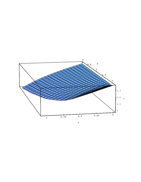
Figure 1: Asymptotically free surface, where the $x,~{}y$ and $z$ axes correspond to $\tilde{\alpha}_{f},~{}\tilde{\alpha}_{\lambda}$ and $\tilde{\alpha}_{t}$, respectively.

Eq. (14) defines GYU boundary conditions holding at $M_{\rm GUT}$. Note that they remain unaffected by soft supersymmetry breaking terms, because the $\beta$-functions are not altered by these terms. To predict observable parameters from GYU, we apply the well-known RG technique. We assume that below $M_{\rm GUT}$ the evolution of couplings is governed by the MSSM and that there exists a unique threshold $M_{\rm SUSY}$ for all superpartners of the MSSM so that below $M_{\rm SUSY}$ the SM is the correct effective theory.

We emphasize that with a GYU boundary condition alone the value of $\tan\beta$ can not be determined. Usually, it is determined in the Higgs sector, which however strongly depends on the supersymmetry braking terms. Here we avoid this by using the tau mass $M_{\tau}$ as an input. As the input data we use $M_{\tau}=1.777~{}\mbox{GeV}~{},~{}M_{Z}=91.188~{}\mbox{GeV}~{},~{}\alpha_{\rm em}^{-1}(M_{Z})=127.9+(8/9\pi)\,\log(M_{t}/M_{Z})~{},~{}\sin^{2}\theta_{\rm W}(M_{Z})=0.2319-3.03\times 10^{-5}T-8.4\times 10^{-8}T^{2}$, where $T=M_{t}/[\mbox{GeV}]-165$. As we can see from (14), the $\tilde{\alpha}_{\lambda}$-dependence of $\tilde{\alpha}_{t}$ and $\tilde{\alpha}_{b}$ are rather weak, and so we present in Table 1 the predictions for three different values of $\tilde{\alpha}_{f}$ with $\tilde{\alpha}_{\lambda}$ fixed at zero only ($M_{\rm SUSY}=500$ GeV):

Fig. 1

$\tilde{\alpha}_{f}$	$\tilde{\alpha}_{t}$	$\tilde{\alpha}_{b}$	$\alpha_{3}(M_{Z})$	$\tan\beta$	$M_{\rm GUT}$ [GeV]	$m_{b}(M_{b})$ [GeV]	$M_{t}$ [GeV]
$0$	$1.369$	$0.969$	$0.1217$	$52.6$	$1.76\times 10^{16}$	$4.59$	$182.6$
$0.6$	$1.187$	$0.816$	$0.1216$	$51.1$	$1.75\times 10^{16}$	$4.64$	$181.0$
$1.075$	$0.972$	$0.572$	$0.1216$	$47.9$	$1.73\times 10^{16}$	$4.72$	$179.0$

$M_{t,b}$ are the pole masses while $m_{b}(M_{b})$ is the running bottom quark mass at its pole mass. The values for $m_{b}(M_{b})$ may suffer from a relatively large correction coming from the superpartner contribution which is not included above. Because of the infrared behavior of the Yukawa couplings [11], the value of $M_{t}$ may be insensitive against the change of $\tilde{\alpha}_{t}$. In Fig. 2 we plot $M_{t}$ against $\tilde{\alpha}_{t}$ with $\tilde{\alpha}_{b}=0.642$ and $M_{\rm SUSY}=500$ GeV fixed, where the reduction solution corresponds to $\tilde{\alpha}_{t}=1.0$.

Figure 2: $M_{t}$ versus $\tilde{\alpha}_{t}$ with fixed $\tilde{\alpha}_{b}$ and $M_{\rm SUSY}$. The reduction solution corresponds to $\tilde{\alpha}_{t}=1$.

From Fig. 2 we see that with increasing experimental accuracy of $M_{t}$ it may become possible to test various GYU models. Detailed studies on this problem will be published elsewhere [13].

Finally we would like to turn our discussion to proton decay. Since the couplings in the minimal model with GYU are strongly constrained, the parameter space for proton decay is also constrained. To see this, we recall that if one includes the threshold effects of superheavy particles [14], the GUT scale $M_{\rm GUT}$ at which $\alpha_{1}$ and $\alpha_{2}$ meet is related to the mass of the superheavy $SU(3)_{C}$-triplet Higgs supermultiplets contained in $H$ and $\overline{H}$ by

$$M_{H} = [\tilde{\alpha}_{f}]^{15/28}\,[\tilde{\alpha}_{\lambda}]^{-5/28}\,M_{\rm GUT}~{}.$$ (15)

This mass $M_{H}$ controls the nucleon decay which is mediated by dimension five operators [15], and non-observation of the nucleon decay requires $M_{H}\mathrel{\mathchoice{\vbox{\offinterlineskip\halign{$\m@th\displaystyle\hfil#\hfil$\cr>\crcr\sim\crcr} }}{\vbox{\offinterlineskip\halign{$\m@th\textstyle\hfil#\hfil$\cr>\crcr\sim\crcr} }}{\vbox{\offinterlineskip\halign{$\m@th\scriptstyle\hfil#\hfil$\cr>\crcr\sim\crcr} }}{\vbox{\offinterlineskip\halign{$\m@th\scriptscriptstyle\hfil#\hfil$\cr>\crcr\sim\crcr} }}}10^{17}$ GeV for $\tan\beta\sim 50$ [16]. Since $M_{\rm GUT}\sim 1.7\times 10^{16}$ GeV and $\tilde{\alpha}_{f}\mathrel{\mathchoice{\vbox{\offinterlineskip\halign{$\m@th\displaystyle\hfil#\hfil$\cr<\crcr\sim\crcr} }}{\vbox{\offinterlineskip\halign{$\m@th\textstyle\hfil#\hfil$\cr<\crcr\sim\crcr} }}{\vbox{\offinterlineskip\halign{$\m@th\scriptstyle\hfil#\hfil$\cr<\crcr\sim\crcr} }}{\vbox{\offinterlineskip\halign{$\m@th\scriptscriptstyle\hfil#\hfil$\cr<\crcr\sim\crcr} }}}1.1$ as one can see from eq. (14) and Table 1, the value of $\tilde{\alpha}_{\lambda}$ has to be less than $\sim 4.4\times 10^{-5}$. Therefore, the reduction solutions that are consistent with the nucleon decay constraint are very close to solution 1, so to the boundary of the asymptotically surface shown in Fig. 2.

4 Dynamical Unification of Couplings

As we have seen, we can construct gauge-Yukawa unified models by applying the principle of reduction of couplings. Though there are certain successes of these models, the reduction principle is associated with no intuitive, physical meaning. Dynamical Unification of Couplings [9], which we are going to explain, could give a reduction of couplings a simple, theoretical meaning. There exists already an example of DUC: Triviality of gauged Higgs-Yukawa systems is widely expected, unless they are completely asymptotically free. It was found[17] that by imposing a certain relation among the gauge, Higgs and Yukawa couplings which are consistent with perturbative renormalizability, it is possible to make the $SU(3)$-gauged Higgs-Yukawa system completely asymptotically free and hence nontrivial. This RG invariant relation among couplings is a consequence of the reduction of couplings. A DUC appears if the couplings in a theory are forced in a dynamically consistent fashion to be related with each other in order for the theory to remain well-defined in the ultraviolet limit.

Figure 3: The evolution of $\alpha$ above $M_{\rm GUT}$; in the $\overline{\rm MS}$ scheme (dashed) and in OPT (solid line).

However, most grand unified theories become asymptotically nonfree, if one attempts to obtain a desired symmetry breaking pattern and a realistic fermion mass matrix by introducing more Higgs fields. The common wisdom is that such theories develop a Landau pole at a high energy scale, a fact which inevitably suggests that the theory is trivial, unless some new physics is entering before the couplings blow up. There exist, however, arguments [20, 9] based on optimized perturbation theory (OPT) [21], indicating that non-abelian gauge theories can have a nontrivial fixed point.. If this is the case, the idea of DUC could be applied to asymptotically nonfree theories, too.

Unification of the gauge couplings in asymptotically nonfree extensions of the SM were previously considered [23]. In contrast to the present idea, it was assumed that the gauge couplings asymptotically diverge so that if one requires the couplings to become strong simultaneously at a certain energy scale, one can predict their low energy values. The difference of two approaches may be illustrated in Fig. 3, which shows the three-loop evolution of the gauge coupling $\alpha$ above $M_{\rm GUT}$ scale in the $\overline{\rm MS}$ scheme and in optimized perturbation theory in the $SO(10)$-gauge theory with $30$ Dirac fermions in the fundamental representation. The existence of a nontrivial fixed point found in OPT and also the possibility of DUC have to be independently verified in different approaches, of course.

References

- [1] J. C. Pati and A. Salam, Phys. Rev. Lett. 31 (1973) 661; H. Georgi and S. L. Glashow, Phys. Rev. Lett. 32 (1974) 438.
- [2] J. Kubo, K. Sibold and W. Zimmermann, Nucl. Phys. B259 (1985) 331.
- [3] D. Kapetanakis, M. Mondragón and G. Zoupanos, Z. Phys. C60 (1993) 181; M. Mondragón and G. Zoupanos, Nucl. Phys. B (Proc. Suppl) 37 C (1995) 98.
- [4] J. Kubo, M. Mondragón and G. Zoupanos, Nucl. Phys. B424 (1994) 291.
- [5] A. J. Parkes and P. C. West, Phys. Lett. 138B (1984) 99; Nucl. Phys. B256 (1985) 340; D. R. T. Jones and A. J. Parkes, Phys. Lett. B160 (1985) 267; D. R. T. Jones and L. Mezinescu, Phys. Lett. B136 (1984) 242; B138 (1984) 293; A. J. Parkes, Phys. Lett. B156 (1985) 73; S. Hamidi, J. Patera and J. H. Schwarz, Phys. Lett. B141 (1984) 349; D. R. T. Jones and S. Raby, Phys. Lett. B143 (1984) 137; S. Hamidi and J. H. Schwarz, Phys. Lett. B147 (1984) 301; J. E. Björkman, D. R. T. Jones and S. Raby, Nucl. Phys. B259 (1985) 503; J. León et al, Phys. Lett. B156 (1985) 66; X. D. Jiang and X. J. Zhou, Phys. Lett. B197 (1987) 156; B216 (1989) 160; I. Jack and D. R. T. Jones, Phys. Lett. B333 (1994) 372.
- [6] A. V. Ermushev, D. I. Kazakov and O. V. Tarasov, Nucl. Phys. B281 (1987) 72; D. I. Kazakov, Mod. Phys. Lett. A2 (1987) 663; Phys. Lett. B179 (1986) 352; C. Lucchesi, O. Piguet and K. Sibold, Helv. Phys. Acta. 61 (1988) 321.
- [7] W. Zimmermann, Commun. Math. Phys. 97 (1985) 211; R. Oehme and W. Zimmermann, Commun. Math. Phys. 97 (1985) 569.
- [8] H. Georgi, H. Quinn, S. Weinberg, Phys. Rev. Lett. 33 (1974) 451.
- [9] J. Kubo, Nontrivial Asymptotically Nonfree Gauge Theories and Dynamical Unification of Couplings, to appear in Phys. Rev. D.
- [10] S. Dimopoulos and H. Georgi, Nucl. Phys. B193 (1981) 150; N. Sakai, Z. Phys. C11 (1981) 153.
- [11] C. T. Hill, Phys. Rev. D24 (1981) 691; C. T. Hill, C. N. Leung and S. Rao, Nucl. Phys. B262 (1985) 517; W. A. Bardeen, M. Carena, S. Pokorski and C. E. M. Wagner, Phys. Lett. B320 (1994) 110.
- [12] M. Bando, T. Kugo, N. Maekawa and H. Nakano, Mod. Phys. Lett. A7 (1992) 3379.
- [13] J. Kubo, M. Mondragón, M. Olechowski and G. Zoupanos, to appear.
- [14] J. Hisano, H. Murayama and T. Yanagida, Phys. Rev. Lett. 69 (1993) 1992; J. Ellis,S. Kelley and D. V. Nanopoulos, Nucl. Phys. B373 (1992) 55; Y. Yamada, Z. Phys. C60 (1993) 83.
- [15] N. Sakai and T. Yanagida, Nucl. Phy. B197 (1982) 533; S. Weinberg, Phys. Rev. D26 (1982) 287.
- [16] J. Hisano, H. Murayama and T. Yanagida, Nucl. Phys. B402 (1993) 46.
- [17] J. Kubo, K. Sibold and W. Zimmermann, Phys. Lett. 220B (1989) 185; J. Kubo, Phys. Lett. 262B (1991) 472.
- [18] M. Harada et al., Prog. Theor. Phys. 92, (1994) 1161.
- [19] K. -I. Kondo, M. Tanabashi and K. Yamawaki, Prog. Theor. Phys. 89 (1993)1249; K. -I. Kondo et al., Prog. Theor. Phys. 91 (1994) 541.
- [20] A. C. Mattingly and P. M. Stevenson, Phys. Rev. Lett. 69 (1992) 1320; Phys. Rev. D D49 (1994) 47.
- [21] P. M. Stevenson, Phys. Rev. D23 (1981) 2916; J. Kubo, S. Sakakibara and P. M. Stevenson, Phys. Rev. D29, 1682 (1984).
- [22] B. Holdom, Phys. Lett. 150B (1985) 301; K. Yamawaki, M. Bando and K. Matumoto, Phys. Rev. Lett. 56 (1986) 1335; T. Akiba, and T. Yanagida, Phys. Lett. 169B (1986) 432; T. Appelquist, D. Karabali and L. C. R. Wijewardhana, Phys. Rev. Lett. 57 (1986) 957.
- [23] L. Maiani, G. Parisi and R. Petronzio, Nucl. Phys. B136 (1978) 115; N. Cabibo and G. R. Farrar, Phys. Lett. 110B (1982) 107; L. Maiani and R. Petronzio, Phys. Lett. B176 (1986) 12; G. Grunberg, Phys. Rev. Lett. 58 (1987) 1180; S. Theisen, N. D. Tracas and G. Zoupanos, Z. Phys. C37 (1988) 597; C. Alacoque, C. Deom and J. Pestieau, Phys. Lett. B228 (1989) 370; D. Kapetanakis, S. Theisen and G. Zoupanos, Phys. Lett. B229 (1989) 248; P. Q Hung, Phys. Rev. D38 (1988) 377; J. P. Derendinger, R. Kaiser and M. Roncadelli, Phys. Lett. B220 (1989) 164; G. Leontaris, C. E. Vayonakis and N. D. Tracas, Mod. Phys. Lett. A4 (1989) 2429; T. Mori, H. Murayama and T. Yanagida, Phys. Rev. D48 (1993) 2995; B. Brahmachari, U. Sarkar and K. Sridhar, Mod. Phys. Lett. A8 (1993) 3349.