UL–NTZ 29/95
The equivalent photon approximation for coherent processes at colliders

Abstract

We consider coherent electromagnetic processes for colliders with short bunches, in particular the coherent bremsstrahlung (CBS). CBS is the radiation of one bunch particles in the collective field of the oncoming bunch. It can be a potential tool for optimizing collisions and for measuring beam parameters. A new simple and transparent method to calculate CBS is presented based on the equivalent photon approximation for this collective field. The results are applied to the $\phi$–factory $DA\Phi NE$. For this collider about $5\cdot 10^{14}dE_{\gamma}/E_{\gamma}$ photons per second are expected in the photon energy $E_{\gamma}$ range from the visible light up to 25 eV.

1 Introduction

One of the important processes at colliding beams is the bremsstrahlung. In the last years, besides of the well-known ordinary (incoherent) bremsstrahlung the coherent radiation at colliders has been widely discussed [1]–[6].

For definiteness, we consider the photon emission by electrons moving through a proton bunch. The ordinary bremsstrahlung dominates for large enough photon energies. If the photon energy becomes sufficiently small, the radiation is determined by the interaction of the electrons with the collective electromagnetic field of the proton bunch. It is known (see, e.g. §77 in [7]) that the properties of this coherent radiation are quite different for electron deflection angles $\theta_{d}$ much larger or much smaller than the typical radiation angle $\theta_{r}\sim 1/\gamma_{e}$ where $\gamma_{e}$ is the electron Lorentz factor.

It is easy to estimate the ratio of these angles. The electric E and magnetic B fields of the proton bunch are approximately equal in magnitude, $|{\bf E}|\approx|{\bf B}|\sim eN_{p}/(l\sigma_{x})$. These fields are transverse and they deflect the electron into the same direction. In such fields the electron moves around a circumference of radius $R\sim\gamma_{e}m_{e}c^{2}/(eB)$ and gets the deflection angle $\theta_{d}\sim l/R$. On the other hand, the radiation angle $\theta_{r}$ corresponds to a length $l_{R}=R/\gamma_{e}\sim m_{e}c^{2}/(eB)$. Therefore, the ratio of these angles is determined by the parameter $\eta$

$$\eta={r_{e}N_{p}\over\sigma_{x}}\sim{\theta_{d}\over\theta_{r}}\sim{l\over l_{R}}\ .$$ (1)

Let us call the proton bunch long if $\eta\gg 1$. The corresponding radiation is usually called beamstrahlung. Its properties are similar to those of the ordinary synchrotron radiation in an uniform magnetic field (see, e.g. [2]).

The proton bunch is called short if $\eta\ll 1$. In this case the electron trajectory remains practically unchanged during the collision. In some respect, the radiation in the short bunch fields is similar to the ordinary bremsstrahlung, therefore we call it coherent bremsstrahlung (CBS). It differs substantially from the beamstrahlung. In most of the colliders the ratio $\eta$ is either much smaller than one (all the $pp$, $\bar{p}p$ and relativistic heavy-ion colliders, some $e^{+}e^{-}$ colliders and B–factories) or of the order of one (e.g. LEP, TRISTAN). Only linear $e^{+}e^{-}$ colliders have $\eta\gg 1$. Therefore, the CBS has a very wide region of applicability.

In the following we discuss for our example the characteristic features of the CBS. In the usual bremsstrahlung the number of photons emitted by electrons is proportional to the number of electrons and protons:

$$dN_{\gamma}\;\propto\;N_{e}\;N_{p}\;{dE_{\gamma}\over E_{\gamma}}\ .$$ (2)

With decreasing photon energies the coherence length $\sim 4\gamma^{2}_{e}\hbar c/E_{\gamma}$ becomes comparable to the length of the proton bunch $l$. At photon energies

$$E_{\gamma}\stackrel{{\scriptstyle<}}{{\sim}}E_{c}=4{\gamma^{2}_{e}\hbar c\over l}$$ (3)

the radiation arises from the interaction of the electron with the proton bunch as a whole, but not with each proton separately. The quantity $E_{c}$ is called the critical photon energy. Therefore the proton bunch is similar to a “particle” with the huge charge $eN_{p}$ and with an internal structure described by the form factor of the bunch. The radiation probability is proportional to $N_{p}^{2}$ and the number of the emitted photons is given by

$$dN_{\gamma}\;\propto\;N_{e}\;N^{2}_{p}\;{dE_{\gamma}\over E_{\gamma}}\ .$$ (4)

The CBS differs strongly from the beamstrahlung in the soft part of its spectrum. As one can see from (4) the total number of CBS photons diverges in contrast to the beamstrahlung for which (as well as for the synchrotron radiation) the total number of photons is finite.

It is useful to discuss shortly the experimental status and possible applications of this new kind of radiation. The ordinary bremsstrahlung is a well-known process. Its large cross section and small angular spread of photons allows to use this radiation for measuring one of the important parameters of a collider – the luminosity (for example, at HERA and LEP). The beamstrahlung has been observed in a single experiment at SLC [3], and it has been demonstrated that it can be used for measuring the transverse bunch size. The main characteristics of the CBS have been calculated recently [4]–[6], and an experiment for its observation is planned in Novosibirsk. It seems that CBS can be a potential tool for optimizing collisions and for measuring beam parameters. Indeed, the bunch length $l$ can be found from the CBS spectrum, because the critical energy (3) is proportional to $1/l$; the horizontal transverse bunch size $\sigma_{x}$ is related to the photon rate $dN_{\gamma}\propto 1/\sigma_{x}^{2}$. Besides, CBS may be very useful for a fast control over an impact parameter between the colliding bunch axes because a dependence of the photon rate on this parameter has a very specific behaviour.

As examples we give here the numbers of CBS photons for a single bunch collision at the $pp$ collider LHC

$$dN_{\gamma}\sim 10^{4}{dE_{\gamma}\over E_{\gamma}}\ \ \ \mbox{at}\ \ \ E_{\gamma}\stackrel{{\scriptstyle<}}{{\sim}}E_{c}=590\ \mbox{eV}\$$ (5)

and at the B–factory KEKB (for $E_{e}=3.5$ GeV)

$$dN_{\gamma}\sim 10^{7}{dE_{\gamma}\over E_{\gamma}}\ \ \ \mbox{at}\ \ \ E_{\gamma}\stackrel{{\scriptstyle<}}{{\sim}}E_{c}=7\ \mbox{keV}\ .$$ (6)

A classical approach to CBS was given in [1]. A quantum treatment of CBS based on the rigorous concept of colliding wave packets and some applications of CBS to modern colliders were considered in [4]–[6]. In this paper we present a new method to calculate the coherent bremsstrahlung at colliding beams based on the equivalent photon approximation (EPA) for the collective electromagnetic field of the oncoming bunch. This method is much more simple and transparent as that previously discussed. Our method allows to calculate not only the classical radiation but to take into account quantum effects in CBS as well. Here we restrict ourselves to applications in the classical limit. CBS is also interesting for relativistic heavy ion colliders, this topic will be discussed in a forthcoming publication [8]. Quantum effects for CBS and coherent pair production will be considered elsewhere [9].

In section 2 we present a qualitative description of the effect. In the next section we derive the expressions for the collective field of a charged bunch as well as the number of equivalent photons. The luminosity and the polarization are discussed in section 4 followed by expressions for the spectrum in the next chapter. In section 6 we apply the obtained formulae for CBS to the case of the $\phi$–factory $DA\Phi NE$.

2 Qualitative description of CBS

We start with the standard calculation of the bremsstrahlung (see [10], §93 and §97) at $ep$ collisions. This process is defined by the block diagram of Fig. 1a, which gives the radiation of the electron.

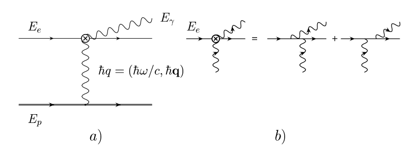
Figure 1: Feynman diagrams for the $ep\to ep\gamma$ process: a) block diagram for bremsstrahlung photon emission by the electron, b) Compton scattering of equivalent photons on the electron.

We denote by $\hbar q$ the 4–momentum of the virtual photon. The main contribution to the cross section is given by the region of small values $(-q^{2})$. In this region the given reaction can be represented as a Compton scattering of the equivalent photon (radiated by the proton) on the electron - Fig. 1b. Therefore, one obtains

$$d\sigma_{ep\to ep\gamma}=dN_{EP}(\omega,E_{p})\,d\sigma_{e\gamma}(\omega,E_{e},E_{\gamma}).$$ (7)

Here $dN_{EP}$ is the number of equivalent photons (EP) generated by the proton

$$dN_{EP}(\omega,E_{p}) \approx {\alpha\over\pi}{d\omega\over\omega}\int^{(-q^{2})_{\max}}_{(-q^{2})_{\min}}{d(-q^{2})\over(-q^{2})}$$ (8)

$$\approx {\alpha\over\pi}{d\omega\over\omega}\ln{m^{2}_{e}\over(m_{p}\hbar\omega/E_{p})^{2}}\ ,$$

where

$$(-q^{2})_{\min}={(m_{p}c)^{2}\omega^{2}\over E_{p}(E_{p}-\hbar\omega)}\approx\left({m_{p}c\omega\over E_{p}}\right)^{2}$$ (9)

is determined by kinematics and $(-q^{2})_{\max}\sim(m_{e}c/\hbar)^{2}$ is given by the dynamical cut–off of the Compton cross section. Therefore, the accuracy of this approximation is logarithmic.

The Compton cross section is of the order of

$$d\sigma_{e\gamma}\sim 2\pi\alpha r^{2}_{e}\;{\omega_{\min}\over\omega}{dE_{\gamma}\over E_{\gamma}}$$ (10)

with the minimal energy of the equivalent photon

$$\hbar\omega_{\min}={m^{2}_{e}c^{4}\over 4E_{e}(E_{e}-E_{\gamma})}\;E_{\gamma}\ .$$ (11)

For the cross section (7) we obtain the estimate

$$d\sigma_{ep\to ep\gamma} \sim 4\alpha r^{2}_{e}{dE_{\gamma}\over E_{\gamma}}\int^{\infty}_{\omega_{\min}}\;d\omega\;{\omega_{\min}\over\omega^{2}}\ln{E_{p}m_{e}\over m_{p}\hbar\omega}$$ (12)

$$\sim 4\alpha r^{2}_{e}\ln{{4E_{e}E_{p}(E_{e}-E_{\gamma})\over m_{e}m_{p}c^{4}\,E_{\gamma}}}\;{dE_{\gamma}\over E_{\gamma}}\ .$$

Just as in the standard calculations we can estimate the number of CBS photons using EPA. Taking into account that the number of EP increases by a factor $\sim N_{p}$ compared to the ordinary bremsstrahlung we get (using $d(-q^{2})\to d^{2}q_{\bot}/\pi$)

$$dN_{EP}\sim N_{p}\;{\alpha\over\pi^{2}}\;{d\omega\over\omega}\;{d^{2}q_{\bot}\over q_{\bot}^{2}}.$$ (13)

Since the impact parameter $\varrho$ is of the order of

$$\varrho_{x}\sim{1\over q_{x}},\ \ \varrho_{y}\sim{1\over q_{y}}$$ (14)

we can rewrite this expression in another form

$$dN_{EP}\sim N_{p}\;{\alpha\over\pi^{2}}\;{d\omega\over\omega}\;{d^{2}\varrho\over\varrho^{2}}\ .$$ (15)

To perform the integration over $\varrho$ we estimate the main integration region as follows. The region of small impact paramaters $|\varrho_{x}|\ll\sigma_{x}$ and $|\varrho_{y}|\ll\sigma_{y}$ does not give a significant contribution because the electromagnetic field vanishes in the centre of a symmetric bunch. The region of large impact parameter $|\varrho_{x}|\gg\sigma_{x}$ and $|\varrho_{y}|\gg\sigma_{y}$ also does not contribute significantly since the proton bunch form factor decreases rapidly. Therefore, the region which gives the main contribution is

$$|\varrho_{x}|\sim|1/q_{x}|\sim\sigma_{x},\;\;\;|\varrho_{y}|\sim|1/q_{y}|\sim\sigma_{y}\ .$$ (16)

Integrating over this region we obtain

$$dN_{EP}\sim N_{p}\;{\alpha\over\pi}\;{d\omega\over\omega}\;{\sigma_{x}\sigma_{y}\over\sigma_{x}^{2}+\sigma_{y}^{2}}\ .$$ (17)

As a result the “effective cross section”  for CBS is of the order of

$$d\sigma_{\rm eff}\sim N_{p}\,\alpha\,r_{e}^{2}\;{\sigma_{x}\sigma_{y}\over\sigma_{x}^{2}+\sigma_{y}^{2}}{dE_{\gamma}\over E_{\gamma}}.$$ (18)

In particular, for flat beams $\sigma_{y}\ll\sigma_{x}$ one has

$$d\sigma_{\rm eff}\sim N_{p}\,\alpha\,r_{e}^{2}\;{\sigma_{y}\over\sigma_{x}}{dE_{\gamma}\over E_{\gamma}}.$$ (19)

To illustrate the transition from the ordinary bremsstrahlung to CBS we present in Fig. 2 qualitatively the photon spectrum for the HERA collider using the results of the last paper in [4].

Figure 2: Effective cross section for the emission of bremsstrahlung photons at HERA as function of the photon energy. The huge increase at low photon energies is due to the coherent bremsstrahlung effect, the high energy tail corresponds to ordinary (incoherent) bremsstrahlung.

In the region of $E_{\gamma}\sim 10$ keV the number of photons dramatically increases by about 9 orders of magnitude.

3 The collective electromagnetic field of a charged bunch and the number of equivalent photons

To define a coordinate frame we choose the $z$–axis along the momentum of the initial electron, the $x$– and $y$–axes in the transverse horizontal and vertical directions, respectively. The possible changes in the transverse sizes of the bunches during the collision are neglected.

The electromagnetic field of a single proton moving with the constant velocity ${\bf v}$ (along $(-z)$–axis) can be found for example in [7], §64. An expansion of this field in plane waves has the form

$${\bf E_{q}}(t) = -4\pi ie{{\bf q}-{\bf v}({\bf qv})/c^{2}\over{\bf q}^{2}-({\bf qv}/c)^{2}}\ \mbox{e}^{-i{\bf qv}t};$$

$${\bf B_{q}}(t) = {{\bf v}\over c}\times{\bf E_{q}}(t).$$ (20)

From that expression one can see that the wave with the wave vector ${\bf q}$ has the frequency

$$\omega={\bf qv}\ .$$ (21)

For such a wave we put in correspondence an equivalent photon with the 4-momentum $\hbar q=(\hbar\omega/c,\hbar{\bf q})$.

Now we consider the field of the whole bunch of protons. If the particle distribution does not change considerably during the collision, the proton density $n_{p}({\bf r},t)$ depends on ${\bf r}$ and $t$ in the following combination only

$$n_{p}({\bf r},t) = n_{p}({\bf r}-{\bf v}t)=n_{p}({\mbox{\boldmath$\varrho$}},z+vt);$$

$${\bf r} = (\mbox{\boldmath$\varrho$},z)=(\varrho_{x},\varrho_{y},z)\ .$$ (22)

Let us define the form factor of the proton bunch density at $t=0$

$$F_{p}({\bf q})=\int n_{p}({\bf r})\;\mbox{e}^{-i{\bf qr}}\;d^{3}r$$ (23)

with its normalization

$$F_{p}(0)=\int n_{p}({\bf r})\;d^{3}r=N_{p}\ .$$ (24)

We find the electric and magnetic fields of the proton bunch analogous to the calculation in the problem of §64 in [7]

$${\bf E}({\bf r},t) = \int{\bf E_{q}}(t)\;F_{p}({\bf q})\ \mbox{e}^{i{\bf qr}}\;{d^{3}q\over(2\pi)^{3}};$$

$${\bf B}({\bf r},t) = {{\bf v}\over c}\times{\bf E}({\bf r},t)$$ (25)

where ${\bf E_{q}}(t)$ is the same as in (20). The spectral expansion of the proton bunch field contains the same frequencies (21). The spectral components of these fields are

$${\bf B}_{\omega}({\bf r})=\int{\bf B}({\bf r},t)\ \mbox{e}^{i\omega t}\;dt=\frac{{\bf v}}{c}\times{\bf E}_{\omega}({\bf r})\ ;$$ (26)

$${\bf E}_{\omega}({\bf r}) = -{4\pi ie\over v}\ \mbox{e}^{iq_{z}z}$$

$$\times \int{{\bf q}-{\bf v}\omega/c^{2}\over{\bf q}_{\bot}^{2}+\omega^{2}/(v\gamma_{p})^{2}}\;F_{p}({\bf q})\ \mbox{e}^{i{\bf q}_{\bot}\mbox{\scriptsize\boldmath$\varrho$}}\;{d^{2}q_{\bot}\over(2\pi)^{2}};$$

$$\gamma_{p} = {1\over\sqrt{1-(v/c)^{2}}}.$$ (27)

The form factor $F_{p}({\bf q})$ decreases rapidly when the components of ${\bf q}$ become larger than the inverse proton bunch sizes. This means that the characteristic values of $\omega/(v\gamma_{p})\sim 1/(l\gamma_{p})$ are much less than those of $q_{\bot}\sim 1/\sigma_{y}$. Therefore, one can omit the quantity $\omega^{2}/(v\gamma_{p})^{2}$ in the integrand of (27).

The electromagnetic field is dominated by its transverse components. For the transverse electric field

$${\bf E}_{\bot}({\bf r},t)=-4\pi ie\int{{\bf q}_{\bot}\over{\bf q}^{2}-(\omega/c)^{2}}\;F_{p}({\bf q})\ \mbox{e}^{i({\bf qr}-\omega t)}\;{d^{3}q\over(2\pi)^{3}}$$

(28)

its spectral component (in which we omit an irrelevant phase factor exp$(iq_{z}z)$ ) has the form

$${\bf E}_{\omega}({\mbox{\boldmath$\varrho$}})=-{4\pi ie\over v}\ \int{{\bf q}_{\bot}\over{\bf q}^{2}_{\bot}}\;F_{p}({\bf q})\ \mbox{e}^{i{\bf q}_{\bot}{\mbox{\scriptsize\boldmath$\varrho$}}}\;{d^{2}q_{\bot}\over(2\pi)^{2}}\ .$$ (29)

The field ${\bf E}_{\bot}({\bf r},t)$ is real, hence $|{\bf E}_{-\omega}({\mbox{\boldmath$\varrho$}})|=|{\bf E}_{\omega}^{*}({\mbox{\boldmath$\varrho$}})|$ from which we get the relation

$$\int^{\infty}_{-\infty}\mid{\bf E}_{\bot}({\bf r},t)\mid^{2}\;dt=2\int^{\infty}_{0}\mid{\bf E}_{\omega}(\mbox{\boldmath$\varrho$})\mid^{2}\;{d\omega\over 2\pi}.$$ (30)

Having calculated the electromagnetic field of the proton bunch we calculate now the number of equivalent photons. The main idea of EPA is that the electromagnetic interaction of an electron with the complicated field of the proton bunch is replaced by a more simple Compton scattering of this electron with the flux of EP generated by the proton bunch.

To perform such a reduction, let us remind a few facts about the collisions of two beams. It is well–known (see, e.g. §12 in [7]) that a number of events for a process with the cross section $\sigma_{12}$ is equal to

$$dN=dL_{12}\ d\sigma_{12};\;\;dL_{12}=(v_{1}+v_{2})n_{1}n_{2}\;d^{3}r\;dt$$ (31)

where $n_{j}$ is the particle density of the $j$-th bunch, $v_{j}$ its velocity and $L_{12}$ the luminosity for a single head–on collision of the bunches. If these densities are of the form (22)

$$n_{1}=n_{1}({\mbox{\boldmath$\varrho$}},z-v_{1}t);\;\;n_{2}=n_{2}({\mbox{\boldmath$\varrho$}},z+v_{2}t)$$ (32)

one can replace $z,\;t$ by the new variables $z-v_{1}t,\;z+v_{2}t$ and integrate the expression (31) independently over these new variables. After these integrations the luminosity depends on the so called “transverse densities”

$$n_{j}({\mbox{\boldmath$\varrho$}})=\int n_{j}\;dz\ .$$ (33)

The transverse density is equal to the total number of corresponding particles which cross a unit area around the impact parameter $\varrho$ during the collision. As a result, the luminosity is

$$dL_{12}=n_{1}({\mbox{\boldmath$\varrho$}})\;n_{2}({\mbox{\boldmath$\varrho$}})\;d^{2}\varrho\ .$$ (34)

Now we can apply these formulae for CBS considering it as the scattering of electrons (index 1) on the electromagnetic field of the proton bunch. Replacing this field by the flux of EP (index 2) with some spectrum we obtain the number of the produced CBS photons in the form

$$dN_{\gamma} = dL_{e\gamma}(\omega)\ d\sigma_{e\gamma}(\omega,E_{\gamma});$$

$$dL_{e\gamma}(\omega) = n_{e}({\mbox{\boldmath$\varrho$}})\ n_{\gamma}({\mbox{\boldmath$\varrho$}},\omega)\ d\omega\ \;d^{2}\varrho\ .$$ (35)

Here $n_{e}({\mbox{\boldmath$\varrho$}})$ is the transverse electron density, $n_{\gamma}({\mbox{\boldmath$\varrho$}},\omega)d\omega$ the transverse density of EP with frequencies in the interval from $\omega$ to $\omega+d\omega$. $dL_{e\gamma}(\omega)$ denotes the differential luminosity for the collisions of electrons and EP and $d\sigma_{e\gamma}(\omega,E_{\gamma})$ is the cross section of the Compton scattering of the electron on the equivalent photon with the frequency $\omega$.

In our case of ultrarelativistic protons ($\gamma_{p}\gg 1$, $v\approx c$) the electric and magnetic fields of the proton bunch (25) are approximately equal, transverse and orthogonal to each other

$${\bf E}\approx{\bf E}_{\bot}\ ,\ \ {\bf B}\approx{\bf B}_{\bot}\ ,\ \ |{\bf E}|\approx|{\bf B}|\ ,\ \ {\bf E\cdot B}=0\ .$$ (36)

Therefore, they are similar to the usual fields describing waves of light. We obtain for the flux of the electromagnetic energy through the unit area around the impact parameter $\varrho$ the known expression

$${c\over 4\pi}\;\int^{\infty}_{-\infty}\mid{\bf E}_{\bot}({\bf r},t)\mid^{2}\;dt\ .$$ (37)

It can be rewritten as the total energy of EP crossing the same area during the collision

$$\int^{\infty}_{0}\hbar\omega\ n_{\gamma}({\mbox{\boldmath$\varrho$}},\omega)\;d\omega\ .$$ (38)

Using (30) we obtain the transverse density of the EP

$$n_{\gamma}({\mbox{\boldmath$\varrho$}},\omega)\;d\omega = {c\over 4\pi^{2}}\;\mid{\bf E}_{\omega}({\mbox{\boldmath$\varrho$}})\mid^{2}\;{d\omega\over\hbar\omega}$$ (39)

$$= 4\alpha\;{d\omega\over\omega}\left|\int{{\bf q}_{\bot}\over{\bf q}^{2}_{\bot}}\;F_{p}({\bf q})\ \mbox{e}^{i{\bf q}_{\bot}\mbox{\scriptsize\boldmath$\varrho$}}\;{d^{2}q_{\bot}\over(2\pi)^{2}}\right|^{2}.$$

It should be noticed that the integration over ${\bf q}_{\bot}$ can be extended to $\infty$ even at $\varrho\to 0$ due to the proper behaviour of the form factor. It provides a high accuracy of our method compared to the usual Weizsäcker–Williams approximation (discussed in section 2) which is correct only logarithmically.

4 Luminosity $L_{e\gamma}$ and polarization of EP

Based on the obtained expression for the equivalent photon number we can calculate the luminosity $L_{e\gamma}$. Substituting (39) into (35) and performing the integration over $\varrho$ we express the luminosity in the form

$$dL_{e\gamma}(\omega)={{\alpha}\over{\pi}}{d\omega\over\omega}J(\omega)$$ (40)

with the function $J(\omega)$ containing both the electron $F_{e}$ and the proton $F_{p}$ bunch form factors

$$J(\omega)=4\pi\int{{\bf q}_{\perp}{\bf q}^{\prime}_{\perp}\over{\bf q}^{2}_{\perp}{{\bf q}^{\prime}_{\perp}}{}^{2}}\;F_{p}({\bf q})F^{*}_{p}({\bf q}^{\prime})F_{e}({\bf q}^{\prime}-{\bf q})\;{d^{2}q_{\perp}d^{2}q^{\prime}_{\perp}\over(2\pi)^{4}}$$

(41)

and

$$q_{z}=q^{\prime}_{z}=-\omega/c.$$ (42)

It is useful to consider in detail the important case of Gaussian beams since usually it is assumed that near the interaction point the particle distribution of the bunches is Gaussian like. In this case the density $n_{p}({\bf r})$ can be represented as a product of the transverse $n_{p}({\mbox{\boldmath$\varrho$}})$ and longitudinal $n_{p}(z)$ densities

$$n_{p}({\bf r}) = n_{p}({\mbox{\boldmath$\varrho$}})\cdot n_{p}(z);\;n_{p}(z)={1\over\sqrt{2\pi}\sigma_{pz}}\;\mbox{exp}\left(-{z^{2}\over 2\sigma^{2}_{pz}}\right);$$

$$l \equiv \sigma_{pz};$$ (43)

$$n_{p}({\mbox{\boldmath$\varrho$}})={N_{p}\over 2\pi\sigma_{px}\sigma_{py}}\;\mbox{exp}\left(-{\varrho_{x}^{2}\over 2\sigma_{px}^{2}}-{\varrho_{y}^{2}\over 2\sigma_{py}^{2}}\right),$$ (44)

and the form factor of the proton bunch is

$$F_{p}({\bf q})=N_{p}\;\mbox{exp}\left[-{1\over 2}(q_{x}\sigma_{px})^{2}-{1\over 2}(q_{y}\sigma_{py})^{2}-{1\over 2}(\omega l/c)^{2}\right].$$

(45)

Analogous formulae take place for the electron bunch replacing the index $p\to e$. In the general case, when the electron bunch axis is shifted by a distance ${\bf R}=(R_{x},R_{y})$ from the proton bunch axis the electron bunch form factor in Eqs. (41), (50) is equal to

$$F_{e}({\bf q}^{\prime}-{\bf q})=N_{e}\;\mbox{exp}\bigg{[}-{1\over 2}(q_{x}^{\prime}-q_{x})^{2}\sigma_{ex}^{2}$$

$$-{1\over 2}(q_{y}^{\prime}-q_{y})^{2}\sigma_{ey}^{2}-i({\bf q}^{\prime}_{\bot}-{\bf q}_{\bot}){\bf R}\bigg{]}\ .$$ (46)

From these expressions we immediately obtain the important relation

$${J(\omega)\over J(0)} = \left|\int n_{p}(z)\mbox{exp}(-iq_{z}z)dz\right|^{2}$$ (47)

$$= \mbox{exp}[-(\omega l/c)^{2}]\ .$$

Now we discuss the polarization of EP. The local polarization of EP is determined by the field ${\bf E}_{\omega}({\mbox{\boldmath$\varrho$}})$. In particular, the unit vector

$${\bf e}={{\bf E}_{\omega}({\mbox{\boldmath$\varrho$}})\over\mid{\bf E}_{\omega}({\mbox{\boldmath$\varrho$}})\mid}$$ (48)

is the local polarization vector of EP, and the matrix $e_{i}e_{k}^{*}$ is the local density matrix of EP. To obtain the average density matrix one has to integrate this local matrix with the luminosity (35) over the impact parameter $\varrho$ and normalize it. With this procedure we obtain

$$<e_{i}e_{k}^{*}>={J_{ik}\over J(\omega)};\;\;i,k=x,y;\;\;J(\omega)=J_{xx}+J_{yy};$$ (49)

$$J_{ik}=4\pi\int{q_{i}q^{\prime}_{k}\over{\bf q}^{2}_{\perp}{{\bf q}^{\prime}_{\perp}}{}^{2}}\;F_{p}({\bf q})F^{*}_{p}({\bf q}^{\prime})F_{e}({\bf q}^{\prime}-{\bf q})\;{d^{2}q_{\perp}d^{2}q^{\prime}_{\perp}\over(2\pi)^{4}}\ .$$

(50)

From the expression (49) we obtain the average Stokes parameters of the equivalent photons describing their linear polarization

$$\xi_{1}={J_{xy}+J_{yx}\over J(\omega)}\ ;\ \ \ \xi_{3}={J_{xx}-J_{yy}\over J(\omega)}\ .$$ (51)

Eqs. (40–42,49,50) are the basic formulae to calculate the CBS. Their accuracy can be estimated in the framework of the general approach developed in [5]. Here we only point out the necessary conditions for their application, namely the bunches should be short and their sizes should not change considerably during the collisions.

To obtain the energy and the angular distribution of the CBS photons and their polarization it is sufficient to calculate the quantities $J(0)$ and $<e_{i}e_{k}^{*}>$. Such a calculation for Gaussian beams has been performed in [5] and below we will use it.

5 Spectrum of CBS photons

To calculate the number of CBS photons as given in Eqs. (35,40) one has to use the known Compton cross section (e.g. , from [11])

$$d\sigma_{e\gamma}=2r_{e}^{2}\ {dE_{\gamma}\over E_{\gamma}}\ {d\varphi\over(1+z)^{3}}\big{[}1+z^{2}$$

$$-2z(\xi_{3}\cos 2\varphi-\xi_{1}\sin 2\varphi)\big{]}\$$ (52)

where

$$z\;=\;(\gamma_{e}\theta)^{2}\ .$$ (53)

Here $\theta$ and $\varphi$ are the polar and azimuthal angles of the CBS photons, respectively. The EP energy $\hbar\omega$ is related to the energy $E_{\gamma}$ and the emission angle $\theta$ of the CBS photon by a simple kinematical relation

$$\hbar\omega=(1+z){E_{\gamma}\over 4\gamma_{e}^{2}(1-E_{\gamma}/E_{e})}\;\ .$$ (54)

Introducing the constant $N_{0}$

$$N_{0}={8\over 3}\;\alpha\;r_{e}^{2}\;J(0)$$ (55)

we obtain the angular–energy distribution for the CBS photons (for unpolarized electrons and after integrating over the azimuthal angle $\varphi$)

$$dN_{\gamma} = {3\over 2}N_{0}{dE_{\gamma}\over E_{\gamma}}{dz\over(1+z)^{2}}$$ (56)

$$\times \left[{1+z^{2}\over(1+z)^{2}}\left(1-{E_{\gamma}\over E_{e}}\right)+{E_{\gamma}^{2}\over 2E_{e}^{2}}\right]\ {J(\omega)\over J(0)}\ .$$

The energy spectrum of CBS photons is obtained by integrating (56) over $z$

$$dN_{\gamma}=N_{0}\;\Phi(E_{\gamma},E_{e})\;{dE_{\gamma}\over E_{\gamma}};$$ (57)

$$\Phi(E_{\gamma},E_{e}) = {3\over 2}\int_{0}^{\infty}{dz\over(1+z)^{2}}$$ (58)

$$\times \left[{1+z^{2}\over(1+z)^{2}}\left(1-{E_{\gamma}\over E_{e}}\right)+{E_{\gamma}^{2}\over 2E_{e}^{2}}\right]\cdot{J(\omega)\over J(0)}\ .$$

The spectral function $\Phi(E_{\gamma},E_{e})$ is normalized by the condition

$$\Phi(0,E_{e})=1\ .$$ (59)

The properties of this spectral function are determined by the ratio $J(\omega)/J(0)$. For Gaussian beams this ratio depends on the longitudinal density of the proton bunch (see Eq. (47)). The constant $N_{0}$ depends on the transverse densities of the electron and proton bunches only.

Now we consider the important case of flat Gaussian beams ($a_{y}^{2}=\sigma_{ey}^{2}+\sigma_{py}^{2}\ll a_{x}^{2}=\sigma_{ex}^{2}+\sigma_{px}^{2}$). In that case the constant $N_{0}$ is equal to [5]

$$N_{0} = {8\over 3\pi}\;\alpha N_{e}\left({r_{e}N_{p}\over a_{x}}\right)^{2}$$ (60)

$$\times {\arcsin(\sigma_{ex}/a_{x})^{2}+\arcsin(\sigma_{ey}/a_{y})^{2}\over[1-(\sigma_{ex}/a_{x})^{4}]^{1/2}},$$

in particular, for flat and identical beams ($\sigma_{x}=\sigma_{ex,px}$, $\sigma_{y}=\sigma_{ey,py}$)

$$N_{0}={8\over 9\sqrt{3}}\;\alpha N_{e}\left({r_{e}N_{p}\over\sigma_{x}}\right)^{2}.$$ (61)

Integrating Eq. (34) over $d^{2}\varrho$ we find the luminosity of $ep$ collisions

$$L_{ep}({\bf R}) = L_{ep}(0)\ \mbox{exp}\left(-{R_{x}^{2}\over 2a^{2}_{x}}-{R_{y}^{2}\over 2a^{2}_{y}}\right);$$

$$L_{ep}(0) = {N_{e}N_{p}\over 2\pi a_{x}a_{y}}$$ (62)

and define the “effective cross section”

$$d\sigma_{\rm eff}={dN_{\gamma}\over L_{ep}}\ .$$ (63)

For the case of identical flat beams and at $R=0$ this quantity is of the form

$$d\sigma_{\rm eff}={32\pi\over 9\sqrt{3}}N_{p}\,\alpha\,r_{e}^{2}\;{\sigma_{y}\over\sigma_{x}}\ \Phi(E_{\gamma},E_{e})\ {dE_{\gamma}\over E_{\gamma}}$$ (64)

in accordance with the estimate (19).

All obtained formulae are valid both in the classical ($E_{c}\ll E_{e}$) and in the quantum ($E_{c}\gg E_{e}$) cases. Below we consider only the classical limit which is valid for all the existing colliders. The quantum effects being at the moment of mainly theoretical interest will be studied in [9].

In the classical case the energy of the CBS photons is $E_{\gamma}\stackrel{{\scriptstyle<}}{{\sim}}E_{c}$. The angular–energy distribution (56) simplifies to the expression

$$dN_{\gamma}={3\over 2}N_{0}{dE_{\gamma}\over E_{\gamma}}\;dz\;{1+z^{2}\over(1+z)^{4}}\ {J(\omega)\over J(0)};$$ (65)

$$\omega={E_{\gamma}\over 4\gamma_{e}^{2}\hbar}\;(1+z)=\frac{E_{\gamma}}{E_{c}}\frac{c}{l}(1+z)\ .$$ (66)

6 Application of CBS to the $DA\Phi NE$ collider

The $DA\Phi NE$ $e^{+}e^{-}$ collider has been proposed in 1990 and it is now under construction at Frascati [12]. The collider is planned to run in 1997 at cms energy of the $\phi$ meson with an initial luminosity of $10^{32}$ cm^-2s^-1. The expected collider parameters are the following [12, 13]

$$N_{e} = N_{e^{+}}=0.89\cdot 10^{11}\ ,\ \ \sigma_{z}=3\ \mbox{cm}\ ,\ \ \sigma_{x}=2\ \mbox{mm}\ ,$$

$$\sigma_{y} = 0.02\ \mbox{mm}\ ,\ \ E_{e}=0.5\ \mbox{GeV}\ .$$ (67)

The parameter $\eta$ from (1) is equal to

$$\eta=0.12$$ (68)

from which follows that $DA\Phi NE$ belongs to the colliders with short bunches for which the photon radiation at small energies is the coherent bremsstrahlung.

6.1 Spectrum of CBS photons

Using the formulae (3) and (61) we find the critical energy $E_{c}$ of CBS photons and the constant $N_{0}$

$$E_{c}=25\ \mbox{eV}\ ,\ \ N_{0}=5.2\cdot 10^{6}\ .$$ (69)

The number of CBS photons for a single collision of the beams is

$$dN_{\gamma}=N_{0}\ \Phi(E_{\gamma}/E_{c}){dE_{\gamma}\over E_{\gamma}}$$ (70)

where the function $\Phi(x)$ is obtained from (58) in the classical limit $E_{c}\ll E_{e}$

$$\Phi(x)={3\over 2}\;\int_{0}^{\infty}{1+z^{2}\over(1+z)^{4}}\;\mbox{exp}[-x^{2}(1+z)^{2}]\;dz\ ,$$ (71)

$$\Phi(x) = 1\;\;\mbox{at}\;\;x\ll 1;$$

$$\Phi(x) = (0.75/x^{2})\cdot\mbox{e}^{-x^{2}}\;\;\mbox{at}\;\;x\gg 1\ .$$ (72)

Some values of this function are: $\Phi(x)=$ 0.80, 0.65, 0.36, 0.10, 0.0023 for $x=$ 0.1, 0.2, 0.5, 1, 2.

It may be convenient for $DA\Phi NE$ to use the CBS photons in the range of the visible light $E_{\gamma}\sim 2-3$ eV $\ll$ 25 eV. In this region the rate of photons is expected to be

$${dN_{\gamma}\over\tau}\approx 5\cdot 10^{14}\;{dE_{\gamma}\over E_{\gamma}}\;\;\;\mbox{photons$\;$ per $\;$ second}$$ (73)

where $\tau=0.0108\;\mu$s is the time between collisions of the bunches at a given interaction region. Additionally, in this energy region the photon polarization should be easily measurable.

To use the CBS photons for monitoring the beams a special window should be installed in the beam pipe. A serious problem for the observation and application of CBS may be the background due to synchrotron radiation on the external magnetic field of the accelerator. This background strongly depends on the details of the magnetic layout of the collider.

6.2 Collisions with a non–zero impact parameter of the bunches

If the electron bunch axis is shifted in the horizontal (vertical) direction by a distance $R_{x}$ ($R_{y}$) from the positron bunch axis, the luminosity decreases exponentially (see Eq. (62)). On the contrary, in the case of a vertical displacement the number of CBS photons increases almost two times (by $92\%$ at $R_{y}=4.0\,\sigma_{y}$). After that, the rate of photons decreases, but even at $R_{y}=15\,\sigma_{y}$ the normalized photon rate reaches $\approx 1.65$. The corresponding curve is presented in Fig. 3.

Figure 3: Normalized photon emission rate at $DA\Phi NE$ in dependence on the displacement $R_{i}$ of the bunch axes. The full and the dotted curves correspond to a displacement in the vertical and horizontal direction, respectively.

The effect does not depend on the photon energy and it can be explained as follows. At $R_{y}=0$ a considerable portion of the electrons moves in the region of small impact parameters where the electric and magnetic fields of the positron bunch are small. For $R_{y}$ in the range of $\sigma_{y}^{2}\ll R_{y}^{2}\ll\sigma_{x}^{2}$ the electrons fly through a stronger electromagnetic field of the positron bunch, therefore, the number of the emitted photons increases. At large $R_{y}$ (for $\sigma_{x}^{2}\ll R_{y}^{2}\ll l^{2}$, not shown in the Fig.), the fields of the positron bunch are $|{\bf E}|\approx|{\bf B}|\propto\;|1/R_{y}|$ which leads to $dN_{\gamma}\propto\;1/R_{y}^{2}$. In that region the number of emitted photons decreases, but very slowly compared with the luminosity.

Shifting the electron bunch axis in the horizontal direction, the positron bunch fields immediately become weaker and the photon rate decreases (see the dotted curve in Fig. 3). However, this decrease is not so strong as that of the luminosity. For example, $dN_{\gamma}(R_{x})/dN_{\gamma}(0)=0.091$ at $R_{x}=5\,\sigma_{x}$, but the luminosity drops by three orders of magnitude.

Such an unusual dependence of the CBS photon rate on ${\bf R}$ can be used for a fast control over impact parameters between beams and over transverse beam sizes. For the case of long round bunches, such an experiment has already been successfully performed at the SLC collider [3].

6.3 Azimuthal asymmetry and polarization

Taking into account the angular distribution of the final photons in the Compton cross section (52), we obtain instead of Eq. (56) the following distribution of CBS photons

$$dN_{\gamma}={3\over 2}N_{0}{dE_{\gamma}\over E_{\gamma}}{dz\over(1+z)^{4}}\ {d\varphi\over 2\pi}\ [1+z^{2}-2z(\xi_{3}\cos{2\varphi}$$

$$-\xi_{1}\sin{2\varphi})]\mbox{exp}\left[-\left((1+z){E_{\gamma}\over E_{c}}\right)^{2}\right]\ .$$ (74)

If the impact parameter between beams ${\bf R}$ is non–zero, an azimuthal asymmetry of the CBS photons appears, which can be used for an additional control over the beams. For increasing $R_{x}$ ($R_{y}$) the electron bunch is shifted into the region where the electric field of the positron bunch is directed almost horizontally (vertically). As a result, the equivalent photons become linearly polarized in the direction of the field. In general, the average degree of the linear polarization is defined by

$$P_{l}=\sqrt{\xi_{1}^{2}+\xi_{3}^{2}}\ .$$ (75)

For identical beams and horizontal or vertical displacements one gets from (51,50) that $\xi_{1}=0$. In Fig. 4, the average longitudinal polarization for $DA\Phi NE$ is presented.

Figure 4: Average longitudinal polarization $P_{l}$ of equivalent photons at $DA\Phi NE$ vs. the displacement $R_{i}$ of the bunch axes. The full and the dotted curves correspond to vertical and horizontal shifts.

Let us define the azimuthal asymmetry of the emitted photons by the relation

$$A={dN_{\gamma}(\varphi=0)-dN_{\gamma}(\varphi=\pi/2)\over dN_{\gamma}(\varphi=0)+dN_{\gamma}(\varphi=\pi/2)}$$ (76)

where the azimuthal angle $\varphi$ is measured with respect to the horizontal plane. It is not difficult to obtain that this quantity does not depend on the photon energy and it is equal to

$$A=\mp{2(\gamma_{e}\theta)^{2}\over 1+(\gamma_{e}\theta)^{4}}\;|\xi_{3}|$$ (77)

for the horizontal (vertical) displacement of the beams (here $\theta$ is the polar angle of the emitted photon). From Fig. 4 one can see that with increasing $R_{x}$ ($R_{y}$) the fraction of photons emitted in the vertical (horizontal) direction becomes greater than the fraction of photons emitted in the horizontal (vertical) direction.

For any displacements the equivalent photons are linearly polarized with the degree $P_{l}$, the CBS photons are also linearly polarized in the same direction. Denoting by $P_{l}^{CBS}$ the average degree of CBS photon polarization, the ratio $P^{CBS}_{l}/P_{l}$ varies in the interval from 0.5 to 1 when $E_{\gamma}$ increases [6] (see the Table 1).

Table 1: Average degree of the polarization of CBS photons for different energies.

$E_{\gamma}/E_{c}$	0	0.2	0.4	0.6
$P^{CBS}_{l}/P_{l}$	0.5	0.7	0.81	0.86
$E_{\gamma}/E_{c}$	0.8	1	1.5	2
$P^{CBS}_{l}/P_{l}$	0.89	0.94	0.96	0.97

Acknowledgements
V.G. Serbo acknowledges support of the Sächsisches Staatsministerium für Wissenschaft und Kunst, of the Naturwissenschaftlich–Theoretisches Zentrum of the Leipzig University and of the Russian Fond of Fundamental Research. R. Engel is supported by the Deutsche Forschungsgemeinschaft under grant Schi 422/1-2.

References

• [1] M. Bassetti, J. Bosser, M. Gygi-Hanney, A. Hoffmann, E. Keil and R. Coisson: IEEE Trans. on Nucl. Science NS-30 (1983) 2182.
• [2] P. Chen: in “An Introduction to Beamstrahlung and Disruption”, ed. by M. Month and S. Turner, Lectures Notes in Physics 296, Berlin, Heidelberg, New York: Springer 1988
• [3] G. Bonvicini et al.: Phys. Rev. Lett. 62 (1989) 2381
• [4] I.F. Ginzburg, G.L. Kotkin, S.I. Polityko and V.G. Serbo: Phys. Rev. Lett. 68 (1992) 788; Phys. Lett. B286 (1992) 392; Z. Phys. C60 (1993) 737
• [5] I.F. Ginzburg, G.L. Kotkin, S.I. Polityko and V.G. Serbo: Yadernaya Fizika (in Russian) 55 (1992) 3310 and 3324
• [6] S.I. Polityko and V.G. Serbo: Phys. Rev E51 (1995) 2493
• [7] L.D. Landau and E.M. Lifshitz: The Classical Theory of Fields, Moscow: Nauka 1988
• [8] R. Engel, A. Schiller and V.G. Serbo: Leipzig University preprint UL–NTZ 30/95 (1995)
• [9] R. Engel, A. Schiller and V.G. Serbo: in preparation
• [10] V.B. Berestetskii, E.M. Lifshitz and L.P. Pitaevskii: Quantum Electrodynamics, Moscow: Nauka 1989
• [11] I.F. Ginzburg, G.L. Kotkin, S.L. Panfil, V.G. Serbo and V.I. Telnov: Nucl. Instr. Meth. 219 (1984) 5
• [12] M. Agnello et al.: Status of the FINUDA Experiment, in The second $DA\Phi NE$ physics handbook (L. Maiani, G. Pancheri, N. Paver Eds.), SIS Laboratori Nazionali di Frascati, Italy 1995
• [13] The Particle Data Group: Review of Particle Properties, Phys. Rev. D50 (1994) 1197