Abstract

We study the effects of the anomalous chromoelectric and chromomagnetic dipole moments of the top quark on the top-pair production, on the top-pair plus 1jet production, and on their ratios, as well as their dependence on the transverse momenta of the top quark and the jet. We also construct CP-odd and $\hat{T}$-odd observables to probe the dispersive part of the chromoelectric form factor of the top quark, and compare their sensitivities in both top-pair and top-pair plus 1 jet production.

I Introduction

The year 1995 with the discovery of the sixth quark – the top quark [1, 2] marks the triumph for the standard model (SM). The future will be an era of looking for physics beyond the SM. There have been many theories that are pointing to different directions. Only new signs of experimental evidence can point to the right theory. After the discovery of the top quark studies of the properties of the top quark will be the major goal of the Tevatron in the next 10 years. In the next run of the Tevatron both the center of mass energy and the luminosity will be upgraded. The center of mass energy will be at $\sqrt{s}=2$ TeV and the yearly luminosity could be as much as 1–5 fb^-1 [3]. After the Tevatron the Large Hadron Collider (LHC) will further examine the properties of the top quark with much higher statistics, and will begin to investigate the ultimate mechanism for the electroweak symmetry breaking.

The top is so heavy that it provides interesting avenues to new physics, via the production [4, 5, 6, 7, 8], decays [9], and their scattering [10]. One interesting property of the top quark is its anomalous chromomagnetic (CMDM) and chromoelectric (CEDM) dipole moments, which will affect the production, decays, and the interactions of the top quark with other particles. In this work we concentrate on the production channel in a $p\bar{p}$ collider to probe the anomalous dipole moments of the top quark in a model-independent way, using an effective Lagrangain approach. The effects of the anomalous dipole moments on top quark production at hadronic colliders have been studied in some details [4, 6, 7, 8]. The study of CP-violating effects in top-pair production due to the CEDM of the top quark were carried out in Refs. [4, 6]. However, it was first suggested by Atwood, Kagan, and Rizzo [7] to use the total cross sections and transverse momentum distributions of top-pair production to constrain the CMDM of the top quark, and later extended in Ref. [8] to include the CEDM also. Here we extend the study to the production of $t\bar{t}$ pair plus 1 jet (denoted by $t\bar{t}j$), and the ratio of $t\bar{t}j$ to $t\bar{t}$ production, as well as their dependence on the transverse momenta of the top quark and the extra jet. This is the first purpose of the paper. The advantages of studying the ratio include (i) the elimination of systematic uncertainties arising from experimental detections, higher order corrections, and the factorization scale, and (ii) the possibility of studying the dependence on the transverse momentum of the extra jet. In this work we use the parameters of the next run at the Tevatron, i.e., $\sqrt{s}=2$ TeV and yearly luminosity of order of a few fb^-1 [3], and throughout the paper we choose the top mass $m_{t}=176$ GeV [1].

The measurement of the electric dipole moments of neutrons and electrons has been a major effort in pursuing CP-violation other than in the kaon system because a nonzero electric dipole moment is a clean signal of CP-violation. Since the top quark is heavy, it can have potentially large couplings to the Higgs bosons of the underlying theory (e.g. multi-Higgs doublet model [11]) that naturally contains CP-violating phases other than the usual CKM phase, and, therefore, the CEDM of the top quark can be potentially large. Thus, probing the CEDM of the top quark is important in searching for CP-violation, and it requires a CP-odd observable. CP-odd observables can further be classified by their $\hat{T}$ behavior, where $\hat{T}$ is the naive time reversal that transforms the kinematic observables according to the time reversal ($t\to-t$) but without interchanging the initial and final states. A CP-odd and $\hat{T}$-even observable can probe the imaginary part of the CEDM form factor of the top quark, while a CP-odd and $\hat{T}$-odd observable can probe the dispersive part [12]. The simplest example of CP-odd and $\hat{T}$-odd observables will be a triple product of 3-momenta. Since at $p\bar{p}$ machines the initial state is a CP eigenstate, a non-zero expectation value for a CP-odd observable is an indication of CP-violation. The second purpose of the paper is to examine the expectation values for some CP-odd and $\hat{T}$-odd observables in $t\bar{t}$ and $t\bar{t}j$ production, and compare their sensitivities.

The organization of the paper is as follows. In Sec. II we write down the effective Lagrangian and detail the calculation method. In Sec. III we show the results of the total and differential cross sections for $t\bar{t}$ and $t\bar{t}j$ production. In Sec. IV we discuss some CP-odd observables that are sensitive to the CEDM of the top quark. We shall conclude in Sec. V. Detail helicity formulas for the calculations are given in the appendix. Finally, we also emphasize that a similar study on the present data of $b$ quark production should be useful in constraining the anomalous dipole moments of the $b$ quark.

II Effective Lagrangian

The effective Lagrangian for the interactions between the top quark and gluons that include the CEDM and CMDM form factors is

$${\cal L}_{\rm eff}=g_{s}\bar{t}T^{a}\left[-\gamma^{\mu}G_{\mu}^{a}+\frac{F_{2}(q^{2})}{4m_{t}}\sigma^{\mu\nu}G_{\mu\nu}^{a}-\frac{iF_{3}(q^{2})}{4m_{t}}\sigma^{\mu\nu}\gamma^{5}G_{\mu\nu}^{a}\right]t\;,$$ (1)

where $T^{a}$ is the SU(3) color matrices, $G_{\mu\nu}^{a}$ is the gluon field strength, $\sigma^{\mu\nu}=\frac{i}{2}[\gamma^{\mu},\gamma^{\nu}]$, and $F_{2}(q^{2})$ and $F_{3}(q^{2})$ are, respectively, the CMDM and CEDM forms factors of the top quark. Since such CEDM and CMDM interactions are not renormalizable, they must originate from some loop exchanges, and they are $q^{2}$ dependent and can develop imaginary parts. But the imaginary parts must vanish at zero momentum transfer, so the imaginary parts are related to terms of dimension greater than five in the effective Lagrangian. Therefore, for our purposes we only consider these form factors to be real, as displayed in Eq. (1). Assuming $|q^{2}|\ll\Lambda$, where $\Lambda$ is the scale of new physics, the form factors can be approximated by

$$F_{2}(q^{2})\approx\kappa,\qquad F_{3}(q^{2})\approx\tilde{\kappa}\qquad{\rm for}\;|q^{2}|\ll\Lambda\;,$$ (2)

where $\kappa$ and $\tilde{\kappa}$ are independent of $q^{2}$. The CEDM of the top quark is then given by $g_{s}\tilde{\kappa}/(2m_{t})$, while CMDM is $g_{s}\kappa/(2m_{t})$. For $\tilde{\kappa}=1$ and $m_{t}=176$ GeV, the CEDM of the top quark is about $5.6\times 10^{-17}g_{s}\cdot{\rm cm}$. In terms of $\kappa$ and $\tilde{\kappa}$ the effective Lagrangian becomes

$${\cal L}_{\rm eff}=g_{s}\bar{t}T^{a}\left[-\gamma^{\mu}G_{\mu}^{a}+\frac{\kappa}{4m_{t}}\sigma^{\mu\nu}G_{\mu\nu}^{a}-\frac{i\tilde{\kappa}}{4m_{t}}\sigma^{\mu\nu}\gamma^{5}G_{\mu\nu}^{a}\right]t\;.$$ (3)

We can then derive the effective interaction of the $ttg$ vertex

$${\cal L}_{t_{i}t_{j}g}=-g_{s}\bar{t}_{j}T^{a}_{ji}\left[\gamma^{\mu}+\frac{i}{2m_{t}}\sigma^{\mu\nu}q_{\nu}(\kappa-i\tilde{\kappa}\gamma^{5})\right]t_{i}\;G_{\mu}^{a}\;,$$ (4)

where $t_{i}(t_{j})$ is the incoming (outgoing) top quark and $q_{\nu}$ is the 4-momentum of the outgoing gluon. The Lagrangian in Eq. (3) also induces a $ttgg$ interaction given by

$${\cal L}_{t_{i}t_{j}gg}=\frac{ig_{s}^{2}}{4m_{t}}\bar{t}_{j}(T^{b}T^{c}-T^{c}T^{b})_{ji}\sigma^{\mu\nu}(\kappa-i\tilde{\kappa}\gamma^{5})t_{i}G_{\mu}^{b}G_{\nu}^{c}\;,$$ (5)

which is absent in the SM. All the ingredients are now ready for the calculation of the parton level cross sections for the production of $t\bar{t}$ and $t\bar{t}j$.

A $t\bar{t}$ Production

The parton-level processes,

$$\begin{array}[]{rcl}q\bar{q}&\rightarrow&t\bar{t}\\ gg&\rightarrow&t\bar{t}\end{array}$$ (6)

including the CEDM and CMDM interactions have been calculated in Ref. [4, 6, 8]. We did an independent calculation and confirmed the analytic results of Ref. [8]. The contributing Feynman diagrams are shown in Fig. 1, where the dressed vertices corresponding to the $ttg$ and $ttgg$ interactions of Eq. (4) and Eq. (5) are marked by a dot. For convenience we present the parton-level cross sections here

$$\frac{d\hat{\sigma}_{q\bar{q}\to t\bar{t}}}{d\hat{t}} = \frac{8\pi\alpha_{s}^{2}}{9\hat{s}^{2}}\left[\frac{1}{2}-v+z-\kappa+\frac{1}{4}(\kappa^{2}-\tilde{\kappa}^{2})+\frac{v}{4z}(\kappa^{2}+\tilde{\kappa}^{2})\right]$$ (7)

$$\frac{d\hat{\sigma}_{gg\to t\bar{t}}}{d\hat{t}} = \frac{\pi\alpha_{s}^{2}}{12\hat{s}^{2}}\biggr{[}\left(\frac{4}{v}-9\right)\left(\frac{1}{2}-v+2z(1-\frac{z}{v})-\kappa(1-\frac{\kappa}{2})\right)$$ (8)

$$+ \frac{1}{4}(\kappa^{2}+\tilde{\kappa}^{2})\left(\frac{7}{z}(1-\kappa)+\frac{1}{2v}(1+\frac{5\kappa}{2})\right)+\frac{1}{16}(\kappa^{2}+\tilde{\kappa}^{2})^{2}\left(-\frac{1}{z}+\frac{1}{v}+\frac{4v}{z^{2}}\right)\biggr{]}\;.$$ (9)

We shall examine the effects of $\kappa$ and $\tilde{\kappa}$ on $t\bar{t}$ production in the next section.

B $t\bar{t}$ plus 1 jet Production

The $t\bar{t}j$ production including the effects of the CEDM and CMDM couplings of the top quark is a new calculation. The reason to extend the $t\bar{t}$ production to $t\bar{t}j$ production is the richer kinematics that can be constructed in the final state. Also, the kick-out of a high $p_{T}$ gluon enables one to probe the $ttg$ vertex in different phase space region. The contributing subprocesses are

1. $q\bar{q}\to t\bar{t}g$

2. $gg\to t\bar{t}g$

3. $q(\bar{q})g\to t\bar{t}q(\bar{q})$

where $q$ denotes a light parton ($u,d,s,c$, or $b$). The contributing Feynman diagrams for the subprocesses (i) and (ii) are shown in Fig. 2 and Fig. 3, respectively. The subprocess (iii) can be obtained from subprocess (i) by a crossing of the $\bar{q}$ in the initial state with the $g$ in the final state. Since the number of diagrams is large in this case it is convenient to use the helicity-amplitude method to sum and square the amplitudes. We use the helicity-amplitude method of Ref. [13]. The expressions for the helicity amplitudes are given in the appendix. We have checked the gauge invariance of the total amplitude and the Lorentz invariance of the amplitude squared. Moreover, by setting $\tilde{\kappa}=\kappa=0$ in our calculations our results agree with the SM results generated by MADGRAPH [14], and the results of Ref. [15].

Before we leave this section, we specify other inputs in our calculations. We use the parton distribution functions of CTEQ (v.3) [16] of which we chose the leading order fit. We also used a simple 1-loop formula for the running coupling constant $\alpha_{s}$ as follows

$$\alpha_{s}(\mu)=\frac{\alpha_{s}(m_{Z})}{1+\frac{33-2n_{f}}{6\pi}\;\alpha_{s}(m_{Z})\;\log\left(\frac{\mu}{m_{Z}}\right)}\;,$$ (10)

where $\alpha_{s}(m_{Z})=0.117$ [17] and $n_{f}$ is the number of active flavors at the scale $\mu$. The scale used in the parton distribution functions and the running coupling constant is chosen to be $\sqrt{m_{t}^{2}+p_{T}^{2}({\rm top})}$. For $t\bar{t}$ production we used the expressions in Eqs. (7) – (8) for the subprocess cross sections, while for $t\bar{t}j$ production we used the helicity amplitudes listed in the appendix. The decays of the top and anti-top quarks can be included with full spin correlation using the helicity amplitude method [13]. The formulas are also given in the appendix.

III Results

A Total cross sections

The total cross sections for $t\bar{t}$ production at the $\sqrt{s}=2$ TeV $p\bar{p}$ collider are shown in Fig. 4, as a contour plot in $\tilde{\kappa}$ and $\kappa$. The SM value given by $\tilde{\kappa}=\kappa=0$ is about 5.2 pb. From Fig. 4 the cross section is symmetric about $\tilde{\kappa}=0$ because $\tilde{\kappa}$ only appears as even powers in the total cross section. This is easy to understand because the total cross section is not a CP-violating observable to separate the CP-violating form factor $\tilde{\kappa}$. Also, the total cross section increases when $\tilde{\kappa}$ moves away from zero. On the other hand, the cross section is not symmetric about $\kappa=0$, but instead, about $\kappa\simeq 0.8$, due to terms linearly proportional to $\kappa$ in the total cross section. Measurements of the total cross section at the Tevatron (Run II) can impose constraints on $(\tilde{\kappa},\kappa)$ plane.

Figure 5 shows the contours of the cross sections of the $t\bar{t}j$ production with $p_{T}(j)>5,10,20$ GeV, respectively, in (a), (b), and (c). Qualitative behaviors are very similar to that of $t\bar{t}$ production. The SM cross sections with $p_{T}(j)>5,10,20$ GeV are 4, 2.5, and 1.3 pb, respectively. Therefore, measurements of $t\bar{t}j$ cross sections can further impose constraints on the $(\tilde{\kappa},{\kappa})$ plane.

The more interesting quantity is the ratio of the two cross sections: $\sigma(t\bar{t}j)/\sigma(t\bar{t})$ with various $p_{T}(j)$ cuts. This ratio is shown in Fig. 6(a), (b), and (c) for $p_{T}(j)>5,10,20$ GeV, respectively. From Fig. 6(a)–(c) we can see that the ratio is smallest around the region ($\tilde{\kappa}=0,{\kappa}=0$). Though the quantitative behaviors of $t\bar{t}j$ production are very similar to $t\bar{t}$ production, there are regions on $(\tilde{\kappa},\kappa)$ plane that the $t\bar{t}j$ production increases proportionately much more than $t\bar{t}$ production, as shown by, e.g., the contours with ratio greater than 1 in Fig. 6(a). This is not unexpected because of extra dressed $ttg$ and $ttgg$ vertices in $t\bar{t}j$ production. Presumably, if a jet of 5 GeV or more can be identified, a very interesting constraint on $(\tilde{\kappa},\kappa)$ plane can be obtained by requiring the cross section of $t\bar{t}j$ production to be less than $t\bar{t}$ production, i.e., by requiring the ratio to be less than 1. More importantly, by requiring $\sigma(t\bar{t}j)$ with a $p_{T}(j)$ cut to be less than a certain fraction of $\sigma(t\bar{t})$, of which both cross sections can be measured in experiments, $(\tilde{\kappa},\kappa)$ can be further constrained.

B Differential Cross Sections

We shall next examine the effects of $\tilde{\kappa}$ and $\kappa$ on differential cross sections. We first show in Fig. 7 the spectra of the transverse momentum of the top quark for some typical values of $(\tilde{\kappa},\kappa)=[(0,0),(1,0),(0,1),(0,-0.5),(1,1)]$. Part (a) is for $t\bar{t}$ production, while (b), (c), and (d) are for $t\bar{t}j$ production with $p_{T}(j)>5,10$, and 20 GeV, respectively. From Fig. 7 we observe the following common features for both $t\bar{t}$ and $t\bar{t}j$ production. The shape of the transverse momentum $p_{T}$ spectrum of the top quark are not sensitive to the CEDM form factor $\tilde{\kappa}$, which only affects the normalization, as indicated by comparing the $(\tilde{\kappa},\kappa)=(0,0)$ and $(1,0)$ curves and by comparing $(0,1)$ and $(1,1)$ curves. It is understood that the simple $p_{T}$ distribution is CP-conserving and, therefore, not sensitive to the CP-violating CEDM form factor $\tilde{\kappa}$. We have also verified that negative and positive $\tilde{\kappa}$’s with the same magnitude produce the same $p_{T}$ spectrum. However, the CMDM form factor $\kappa$ affects the shape of the $p_{T}$ spectrum in a non-trivial way. A positive $\kappa$ enhances the $p_{T}$ spectrum in the large $p_{T}$ region, thus, making the $p_{T}$ spectrum significantly harder than the SM result that should be detectable, as shown by the $(\tilde{\kappa},\kappa)=(0,1),(1,1)$ curves in Fig. 7. On the other hand, a negative $\kappa$ does not affect the shape of the $p_{T}$ spectrum appreciably, as shown by the $(0,-0.5)$ curve. Therefore, by measuring the $p_{T}$ spectrum information on $\kappa$ can be obtained. We also note that the relative shapes of the $p_{T}$ spectra are the same for $t\bar{t}$ and $t\bar{t}j$ production with different $p_{T}(j)$ cuts. In other words, the effects of CEDM and CMDM form factors on the $p_{T}$ spectrum of $t\bar{t}$ production are about the same whether or not an extra jet is tagged. In Fig. 8 we show the rapidity distribution of the top quark for the same set of $(\tilde{\kappa},\kappa)$. The shape of the rapidity spectrum of the top quark is not sensitive to both $\tilde{\kappa}$ and $\kappa$ that only the normalization is affected, as indicated in Fig. 8. Also, the relative positions of the $y$ spectra are about the same for $t\bar{t}$ and $t\bar{t}j$ production with various $p_{T}(j)$ cuts. In Fig. 9 we show the transverse momentum and rapidity distributions of the jet in the $t\bar{t}j$ production, with the same set of $(\tilde{\kappa},\kappa)$. Qualitatively, the various $(\tilde{\kappa},\kappa)$ curves of the $p_{T}(j)$ and $y(j)$ distributions are similar in shape. This fact explains why the relative shapes of the $p_{T}$ spectra in Fig. 7 and the relative positions of the $y$ spectra in Fig. 8 are about the same for $t\bar{t}$ production and $t\bar{t}j$ production with different $p_{T}(j)$ cuts.

The conclusion of studying the total cross sections and differential distributions is that we did not gain better sensitivities to $\tilde{\kappa}$ and $\kappa$ by tagging an extra jet in $t\bar{t}$ production. However, by requiring the cross section of $t\bar{t}j$ production to be less than a certain fraction of $t\bar{t}$ production under a $p_{T}(j)$ cut, of which both cross sections can be measured in experiments, one can constrain $(\tilde{\kappa},\kappa)$.

IV CP-Observables

In the last section, we have shown that the distributions for CP-even observables such as $p_{T}$ are not sensitive to $\tilde{\kappa}$. Moreover, higher order corrections can render the detection by such distributions useless. Only unless $\tilde{\kappa}$ is very large can the effects be detected. Thus, in this section we shall look at some CP-odd observables, which should be sensitive to the CEDM of the top quark and safe from higher order corrections. A nonzero expectation value for such a CP-odd observable at the Tevatron should be a signal for CP-violation, because the initial state $p\bar{p}$ is a CP eigenstate and, also, its expectation value is not affected by the CP-even higher order corrections.

In our effective Lagrangian, since we have assumed $\tilde{\kappa}$ to be real only those CP-odd and $\hat{T}$-odd variables can probe $\tilde{\kappa}$. CP-odd and $\hat{T}$-even variables can only probe the imaginary part of $\tilde{\kappa}$, but such an imaginary part must vanish at zero momentum transfer, so it must be related to terms of higher dimension ($>5$) in the effective Lagrangian.

In the last section, the cross sections for $t\bar{t}$ and $t\bar{t}j$ production are shown for the case that the top helicities are summed. From Eqs. (7)–(8) or from the contour plots we can see that the total cross sections do not contain terms linearly proportional to $\tilde{\kappa}$. Therefore, the total cross section is not sensitive to CP-odd observables when the top helicities are summed. However, it was shown in Ref. [4] that when the top helicities are not summed the cross section does have terms linearly proportional to $\tilde{\kappa}$. In other words, in order to detect the CP-violating effects due to $\tilde{\kappa}$ one needs to have information about the top helicities. Fortunately, the top is so heavy that it decays before hadronization takes place [18] and, therefore, the spin information of the top quark is retained in the decay products. The top helicities or polarizations are not directly measured but can be realized in its weak decay [12, 19], because of the left-handed nature of the weak interaction. Since the top is heavy, in its rest frame the top quark first decays into a $b$ quark and $W^{+}$ boson, with the $b$ preferentially left-handed and the $W^{+}$ boson predominately longitudinal. Due to angular momentum conservation the longitudinal $W^{+}$ boson is preferentially produced along with the direction of the top quark polarization. Therefore, the anti-lepton $\ell^{+}$ produced in the $W^{+}$ decay also prefers to be in the direction of the top polarization. Similarly, the momentum of the lepton $\ell^{-}$ produced in the anti-top decay prefers to be in the opposite direction of the anti-top polarization. Thus, by discriminating the directions of the lepton and anti-lepton one can select particular polarizations of the top and anti-top. Similarly, this argument can also be applied to the $b$ quark and $\bar{b}$ antiquark. We shall look at the following variables [4, 6]:

$$v_{1} = {\bf\hat{p}}\cdot({\bf l^{+}}\times{\bf l^{-}})\;{\bf\hat{p}}\cdot({\bf l^{+}}-{\bf l^{-}})/m_{t}^{3}\;,$$ (11)

$$v_{2} = ({\bf l^{+}}-{\bf l^{-}})\cdot({\bf b}\times{\bf\bar{b}})/m_{t}^{3}\;,$$ (12)

$$v_{3} = \epsilon_{\mu\nu\rho\sigma}\,{\ell^{+}}^{\mu}\,{\ell^{-}}^{\nu}\,b^{\rho}\,\bar{b}^{\sigma}/m_{t}^{4}\;,$$ (13)

$$v_{4} = {\bf\hat{p}}\cdot({\bf b}\times{\bf\bar{b}})\;{\bf\hat{p}}\cdot({\bf b}-{\bf\bar{b}})/m_{t}^{3}\;,$$ (14)

where $\epsilon_{0123}=-1$, and ${\bf l^{+},l^{-},b,\bar{b}}$ represent the 3-momenta of the leptons and quarks , and $\ell^{+},\ell^{-},b,\bar{b}$ represent the 4-momenta of the leptons and quarks, and ${\bf\hat{p}}$ is the unit vector of the proton. Since the initial state of the collision is $p\bar{p}$, which is a CP-eigenstate, nonzero expectation values for these variables are signals of CP-violation. Some of these variables, as signals of CP-violation due to the CEDM of the top, have been demonstrated for $t\bar{t}$ production in Ref. [4, 6]. Our aim is to compare the sensitivities of the $t\bar{t}$ and $t\bar{t}j$ production to these CP-odd observables. We shall put $\kappa=0$ in the following, as it does not affect the expectation value of these CP-odd observables.

We put in the semileptonic decays of the top and anti-top using the helicity amplitude method with full spin correlation (described in the appendix.) In order to detect the leptons and quarks we impose a set of minimal cuts:

$$p_{T}(\ell,b)>5\;{\rm GeV}\qquad|y(\ell,b)|<2\;.$$ (15)

We calculate numerically the expectation values of these observables for $\tilde{\kappa}$ between $-1$ and 1 with an increment of 0.1 or 0.2. The asymmetry $A_{v}$ for a variable $v$ is defined as

$$A_{v}=\frac{\langle v\rangle}{\sqrt{\langle v^{2}\rangle}}$$ (16)

where the expectation value $\langle v\rangle=\int v\frac{d\sigma}{dv}dv/\int\frac{d\sigma}{dv}dv$. Therefore, the expectation values $\langle v\rangle$ and $\langle v^{2}\rangle$ do not scale with the total cross sections or with the branching ratios of the top and anti-top quarks.  The number of signal events due to this asymmetry is $NA_{v}$, where $N$ is the total number of events, and $\sqrt{N}$ is the standard deviation of statistical fluctuation. Therefore, the condition for the signal of the asymmetry to have a $\eta$ sigma significance is given by

$$\sqrt{N}\,A_{v}\geq\eta\qquad{\rm or}\qquad\sqrt{N}\,\frac{\langle v\rangle}{\sqrt{\langle v^{2}\rangle}}\geq\eta\;.$$ (17)

We shall first give the results for $t\bar{t}$ production. For $\tilde{\kappa}$ between $-1$ and 1, the expectation values $\langle v_{i}\rangle$ and $\sqrt{\langle v_{i}^{2}\rangle}$ can be expressed as

$$\begin{array}[]{rcl}\langle v_{1}\rangle=-0.0037\tilde{\kappa}+7.3\times 10^{-5}\tilde{\kappa}^{2}+0.0015\tilde{\kappa}^{3}\,,&&\sqrt{\langle v_{1}^{2}\rangle}\simeq 0.046\;,\\ \langle v_{2}\rangle=0.0040\tilde{\kappa}-1.7\times 10^{-5}\tilde{\kappa}^{2}-0.0015\tilde{\kappa}^{3}\,,&&\sqrt{\langle v_{2}^{2}\rangle}\simeq 0.11\;,\\ \langle v_{3}\rangle=0.0056\tilde{\kappa}-7.6\times 10^{-5}\tilde{\kappa}^{2}-0.0021\tilde{\kappa}^{3}\,,&&\sqrt{\langle v_{3}^{2}\rangle}\simeq 0.07\;,\\ \langle v_{4}\rangle=-0.0018\tilde{\kappa}+7.4\times 10^{-5}\tilde{\kappa}^{2}+0.00075\tilde{\kappa}^{3}\,,&&\sqrt{\langle v_{4}^{2}\rangle}\simeq 0.09\;,\end{array}$$ (18)

where we fitted the numerical results using a polynomial in $\tilde{\kappa}$ up to $\tilde{\kappa}^{3}$. For sufficiently small $\tilde{\kappa}$ only the first term linear in $\tilde{\kappa}$ is important. The $\sqrt{\langle v_{i}^{2}\rangle}$ are roughly independent of $\tilde{\kappa}$ for $\tilde{\kappa}$ between $-1$ and 1. To test the sensitivity of each observable to $\tilde{\kappa}$ we require a 1 sigma effect ($\eta=1$) of the signal, and by Eq. (17) $|\tilde{\kappa}|$ must be larger than a minimum value, given by

$$|\tilde{\kappa}|\geq\left\{\begin{array}[]{ll}\frac{12}{\sqrt{N}}&{\rm for}\;v_{1}\\ \frac{27}{\sqrt{N}}&{\rm for}\;v_{2}\\ \frac{12}{\sqrt{N}}&{\rm for}\;v_{3}\\ \frac{50}{\sqrt{N}}&{\rm for}\;v_{4}\end{array}\right.\;,$$ (19)

where we assumed only the linear term in $\tilde{\kappa}$ in Eq. (18). We can immediately see that the observables $v_{1}$ and $v_{3}$ are about the same in sensitivity to $\tilde{\kappa}$, and more sensitive than $v_{2}$ and $v_{4}$.

For $t\bar{t}j$ production we only give results on $v_{1}$ and $v_{3}$ with $p_{T}(j)>5,10,20$ GeV. The results for the expectation values of $v_{1}$ and $v_{3}$ are:

$$\langle v_{1}\rangle=\left\{\begin{array}[]{ll}-0.0032\tilde{\kappa}-1.4\times 10^{-4}\tilde{\kappa}^{2}+0.0020\tilde{\kappa}^{3}&{\rm for}\;p_{T}(j)>5\,{\rm GeV}\\ -0.0028\tilde{\kappa}-2.1\times 10^{-4}\tilde{\kappa}^{2}+0.0016\tilde{\kappa}^{3}&{\rm for}\;p_{T}(j)>10\,{\rm GeV}\\ -0.0030\tilde{\kappa}-7.7\times 10^{-6}\tilde{\kappa}^{2}+0.0019\tilde{\kappa}^{3}&{\rm for}\;p_{T}(j)>20\,{\rm GeV}\end{array}\right.,\qquad\sqrt{\langle v_{1}^{2}\rangle}\simeq 0.046$$ (20)

$$\langle v_{3}\rangle=\left\{\begin{array}[]{ll}0.0032\tilde{\kappa}-3.6\times 10^{-4}\tilde{\kappa}^{2}-0.0015\tilde{\kappa}^{3}&{\rm for}\;p_{T}(j)>5\,{\rm GeV}\\ 0.0033\tilde{\kappa}-3.7\times 10^{-4}\tilde{\kappa}^{2}-0.0018\tilde{\kappa}^{3}&{\rm for}\;p_{T}(j)>10\,{\rm GeV}\\ 0.0032\tilde{\kappa}-3.6\times 10^{-4}\tilde{\kappa}^{2}-0.0018\tilde{\kappa}^{3}&{\rm for}\;p_{T}(j)>20\,{\rm GeV}\end{array}\right.\qquad\sqrt{\langle v_{3}^{2}\rangle}\simeq 0.07$$ (21)

We can see that the sensitivities of $\langle v_{1}\rangle$ and $\langle v_{3}\rangle$ are about the same for various $p_{T}(j)$ cuts at small $\tilde{\kappa}$ . But, both $\langle v_{1}\rangle$ and $\langle v_{3}\rangle$ are less sensitive to $\tilde{\kappa}$ in $t\bar{t}j$ production than in $t\bar{t}$ production, since the expectation value $\langle v\rangle$ is getting smaller while $\sqrt{\langle v^{2}\rangle}$ remains the same. We have also verified that $v_{2}$ and $v_{4}$ have similar behavior. In general, the sensitivities of the CP-odd observables under consideration decrease when going from $t\bar{t}$ production to $t\bar{t}j$ production, especially, for the observables $v_{2}$, $v_{3}$, and $v_{4}$ that require the $b$ quark and $\bar{b}$ antiquark momenta.

V Conclusions

In this paper, we have studied the effects of the CEDM and CMDM couplings of the top quark on the $t\bar{t}$ and $t\bar{t}j$ production, as well as the ratio of these two cross sections at the Tevatron with $\sqrt{s}=2$ TeV. We found that by demanding $\sigma(t\bar{t}j)$ to be less than a certain fraction of $\sigma(t\bar{t})$ we can obtain constraints on $\tilde{\kappa}$ and $\kappa$. We have also shown that the shape of the differential distributions ($p_{T}$ and $y$) is not sensitive to the CEDM form factor $\tilde{\kappa}$ because these distributions are CP-even. However, the $p_{T}$ distribution is very sensitive to the sign of the CMDM form factor $\kappa$. A positive $\kappa$ significantly hardens the $p_{T}$ spectrum while a negative $\kappa$ does not. Therefore, by measuring the $p_{T}$ spectrum of the top quark we can put bounds on $\kappa$.

Furthermore, we have also studied the effects of $\tilde{\kappa}$ on the expectation values of some CP-odd and $\hat{T}$-odd observables in both $t\bar{t}$ and $t\bar{t}j$ production. The asymmetry $A_{v}$ obtained for these observables ranges between $(2-8)\times 10^{-2}\tilde{\kappa}$. The SM cross section for $t\bar{t}$ production with both the top and anti-top decaying semileptonically is about 0.25 pb. With a luminosity of, say, 5 fb^-1, there are totally of order 1200 events. Using 1-sigma effect as the discovery criterion, it can probe the region $|\tilde{\kappa}|\gtrsim 0.35$ (using Eq. (19)). In other words, if no effect is observed, we can constrain $|\tilde{\kappa}|\lesssim 0.35$. Also, we found that the sensitivities obtained in $t\bar{t}j$ production are smaller than in $t\bar{t}$ production. Therefore, it is not advantageous to tag an extra jet in $t\bar{t}$ production with respect to these CP-odd observables. Since it is very often to have extra jets in $t\bar{t}$ production, the results obtained for the CP-odd observables in $t\bar{t}$ production will be very often contaminated by the smaller results of the $t\bar{t}j$ production. In reality, the experimental measurement will be somewhere in between the results of $t\bar{t}$ and $t\bar{t}j$ production. In this work, we do not consider the effects of gluon radiating off the decay products of the top quark. These effects will also be complicated by the finite width of the top quark. However, we do not expect any significant changes on our conclusions.

A

In this appendix we shall list all helicity amplitudes for the processes (i) $q\bar{q}\to Q\bar{Q}g$, and (ii) $gg\to Q\bar{Q}g$, where $Q$ stands for $t$ or $b$.

1 $q_{i}(p_{1})\;\bar{q}_{j}(p_{2})\;\to Q_{k}(k_{1})\bar{Q}_{l}(k_{2})g_{a}(g)$

The momenta of the particles are labeled in the parentheses and the subscripts denote the color indices of the quarks and the gluon. The contributing Feynman diagrams are shown in Fig. 2. We list the helicity amplitudes for each diagram but without the color factors, which we shall sum later. We use the following short-hand notations:

$$\hat{s}=(p_{1}+p_{2})^{2}\,,\qquad\hat{s}^{\prime}=(k_{1}+k_{2})^{2}\,,\qquad J_{\rho}=\bar{v}(p_{2})\gamma_{\rho}u(p_{1})\;,$$ (A1)

$$\Gamma_{\mu}(p,q;\epsilon_{1},\epsilon_{2})=(p-q)_{\mu}\,\epsilon_{1}\cdot\epsilon_{2}+(p+2q)\cdot\epsilon_{1}\;\epsilon_{2\mu}-(2p+q)\cdot\epsilon_{2}\;\epsilon_{1\mu}\;.$$ (A2)

We also define the following

$$S(p,q)=\overlay{/}{p}+\frac{1}{4m_{Q}}\left(\overlay{/}{p}\overlay{/}{q}-\overlay{/}{q}\overlay{/}{p}\right)\left(\kappa-i\tilde{\kappa}\gamma^{5}\right)$$ (A3)

where $p,q$ are 4-vectors, or if $p$ or $q$ is an index it represents a gamma matrix. The helicity amplitudes are given by

$${\cal M}_{a} = \frac{g_{s}^{3}}{\hat{s}}\bar{u}(k_{1})\,S(\epsilon(g),-g)\,\frac{\overlay{/}{k}_{1}+\overlay{/}{g}+m_{Q}}{(k_{1}+g)^{2}-m_{Q}^{2}}\,S(\rho,p_{1}+p_{2})\,v(k_{2})\;J_{\rho}\;,$$ (A4)

$${\cal M}_{b} = \frac{g_{s}^{3}}{\hat{s}}\bar{u}(k_{1})\,S(\rho,p_{1}+p_{2})\,\frac{-\overlay{/}{k}_{2}-\overlay{/}{g}+m_{Q}}{(k_{2}+g)^{2}-m_{Q}^{2}}\,S(\epsilon(g),-g)\,v(k_{2})\;J_{\rho}\;,$$ (A5)

$${\cal M}_{c} = \frac{g_{s}^{3}}{\hat{s}\hat{s}^{\prime}}\bar{u}(k_{1})\,S(\rho,k_{1}+k_{2})\,v(k_{2})\;\Gamma_{\rho}\left(p_{1}+p_{2},-g;J,\epsilon(g)\right)\;,$$ (A6)

$${\cal M}_{d} = \frac{g_{s}^{3}}{\hat{s}^{\prime}}\bar{u}(k_{1})\,S(\rho,k_{1}+k_{2})\,v(k_{2})\;\bar{v}(p_{2})\gamma_{\rho}\,\frac{\overlay{/}{p}_{1}-\overlay{/}{g}}{(p_{1}-g)^{2}}\,\overlay{/}{\epsilon}(g)\,u(p_{1})\;,$$ (A7)

$${\cal M}_{e} = \frac{g_{s}^{3}}{\hat{s}^{\prime}}\bar{u}(k_{1})\,S(\rho,k_{1}+k_{2})\,v(k_{2})\;\bar{v}(p_{2})\,\overlay{/}{\epsilon}(g)\,\frac{-\overlay{/}{p}_{2}+\overlay{/}{g}}{(-p_{2}+g)^{2}}\,\gamma_{\rho}\,u(p_{1})\;,$$ (A8)

$${\cal M}_{f} = \frac{g_{s}^{3}}{4m_{Q}\hat{s}}\bar{u}(k_{1})\,\left(\overlay{/}{\epsilon}(g)\gamma^{\rho}-\gamma^{\rho}\overlay{/}{\epsilon}(g)\right)\left(\kappa-i\tilde{\kappa}\gamma^{5}\right)\,v(k_{2})\;J_{\rho}\;,$$ (A9)

where $\epsilon(g)$ is the polarization 4-vector of the gluon. Taking into account the color factors the total amplitude can be written as

$${\cal M}=\sum_{\alpha=1}^{4}O_{\alpha}{\cal M}_{\alpha}$$

with

$$O_{1}=(T^{a}T^{b})_{kl}T^{b}_{ji}\,, O_{3}=T^{b}_{kl}(T^{b}T^{a})_{ji}\,,$$ (A10)

$$O_{2}=(T^{b}T^{a})_{kl}T^{b}_{ji}\,, O_{4}=T^{b}_{kl}(T^{a}T^{b})_{ji}\,,$$ (A11)

and

$${\cal M}_{1}={\cal M}_{a}+{\cal M}_{f}\,, {\cal M}_{3}={\cal M}_{d}-{\cal M}_{c}\,,$$ (A12)

$${\cal M}_{2}={\cal M}_{b}-{\cal M}_{f}\,, {\cal M}_{4}={\cal M}_{e}+{\cal M}_{c}\,.$$ (A13)

After squaring and summing all the color factors we have

$$\sum_{\rm color}|{\cal M}|^{2} = \frac{8}{3}\left(|{\cal M}_{1}|^{2}+|{\cal M}_{2}|^{2}+|{\cal M}_{3}|^{2}+|{\cal M}_{4}|^{2}\right)$$ (A14)

$$+ \frac{7}{3}\left({\cal M}_{1}{\cal M}_{3}^{*}+{\cal M}_{1}^{*}{\cal M}_{3}+{\cal M}_{2}{\cal M}_{4}^{*}+{\cal M}_{2}^{*}{\cal M}_{4}\right)$$ (A15)

$$- \frac{2}{3}\left({\cal M}_{1}{\cal M}_{4}^{*}+{\cal M}_{1}^{*}{\cal M}_{4}+{\cal M}_{2}{\cal M}_{3}^{*}+{\cal M}_{2}^{*}{\cal M}_{3}\right)$$ (A16)

$$- \frac{1}{3}\left({\cal M}_{1}{\cal M}_{2}^{*}+{\cal M}_{1}^{*}{\cal M}_{2}+{\cal M}_{3}{\cal M}_{4}^{*}+{\cal M}_{3}^{*}{\cal M}_{4}\right)$$ (A17)

2 $g_{a}(g_{1})\,g_{b}(g_{2})\,\to Q_{i}(k_{1})\,\bar{Q}_{j}(k_{2})\,g_{c}(g)$

The contributing Feynman diagrams are shown in Fig. 3. The helicity amplitudes without the color factors for each diagram are given by

$${\cal M}_{a} = -g_{s}^{3}\bar{u}(k_{1})\,S(\epsilon(g),-g)\,\frac{\overlay{/}{k}_{1}+\overlay{/}{g}+m_{Q}}{(k_{1}+g)^{2}-m_{Q}^{2}}\,S(\epsilon(g_{1}),g_{1})\,\frac{-\overlay{/}{k}_{2}+\overlay{/}{g}_{2}+m_{Q}}{(k_{2}-g_{2})^{2}-m_{Q}^{2}}\,S(\epsilon(g_{2}),g_{2})\,v(k_{2})\;,$$ (A18)

$${\cal M}_{b} = -g_{s}^{3}\bar{u}(k_{1})\,S(\epsilon(g_{1}),g_{1})\,\frac{\overlay{/}{k}_{1}-\overlay{/}{g}_{1}+m_{Q}}{(k_{1}-g_{1})^{2}-m_{Q}^{2}}\,S(\epsilon(g),-g)\,\frac{-\overlay{/}{k}_{2}+\overlay{/}{g}_{2}+m_{Q}}{(k_{2}-g_{2})^{2}-m_{Q}^{2}}\,S(\epsilon(g_{2}),g_{2})\,v(k_{2})\;,$$ (A19)

$${\cal M}_{c} = -g_{s}^{3}\bar{u}(k_{1})\,S(\epsilon(g_{1}),g_{1})\,\frac{\overlay{/}{k}_{1}-\overlay{/}{g}_{1}+m_{Q}}{(k_{1}-g_{1})^{2}-m_{Q}^{2}}\,S(\epsilon(g_{2}),g_{2})\,\frac{-\overlay{/}{k}_{2}-\overlay{/}{g}+m_{Q}}{(k_{2}+g)^{2}-m_{Q}^{2}}\,S(\epsilon(g),-g)\,v(k_{2})\;,$$ (A20)

$${\cal M}_{d} = -\frac{g_{s}^{3}}{(g_{1}-g)^{2}}\,\bar{u}(k_{1})\,S(\rho,g_{1}-g)\,\frac{-\overlay{/}{k}_{2}+\overlay{/}{g}_{2}+m_{Q}}{(k_{2}-g_{2})^{2}-m_{Q}^{2}}\,S(\epsilon(g_{2}),g_{2})\,v(k_{2})\;\Gamma_{\rho}(g_{1},-g;\epsilon(g_{1}),\epsilon(g))\;,$$ (A21)

$${\cal M}_{e} = -\frac{g_{s}^{3}}{(g_{2}-g)^{2}}\,\bar{u}(k_{1})\,S(\epsilon(g_{1}),g_{1})\,\frac{\overlay{/}{k}_{1}-\overlay{/}{g}_{1}+m_{Q}}{(k_{1}-g_{1})^{2}-m_{Q}^{2}}\,S(\rho,g_{2}-g)\,v(k_{2})\;\Gamma_{\rho}(g_{2},-g;\epsilon(g_{2}),\epsilon(g))\;,$$ (A22)

$${\cal M}_{f} = -\frac{g_{s}^{3}}{4m_{Q}}\,\bar{u}(k_{1})\,\left(\overlay{/}{\epsilon}(g)\overlay{/}{\epsilon}(g_{1})-\overlay{/}{\epsilon}(g_{1})\overlay{/}{\epsilon}(g)\right)\left(\kappa-i\tilde{\kappa}\gamma^{5}\right)\,\frac{-\overlay{/}{k}_{2}+\overlay{/}{g}_{2}+m_{Q}}{(k_{2}-g_{2})^{2}-m_{Q}^{2}}\,S(\epsilon(g_{2}),g_{2})\,v(k_{2})\;$$ (A23)

$${\cal M}_{g} = -\frac{g_{s}^{3}}{4m_{Q}}\,\bar{u}(k_{1})\,S(\epsilon(g_{1}),g_{1})\,\frac{\overlay{/}{k}_{1}-\overlay{/}{g}_{1}+m_{Q}}{(k_{1}-g_{1})^{2}-m_{Q}^{2}}\,\left(\overlay{/}{\epsilon}(g_{2})\overlay{/}{\epsilon}(g)-\overlay{/}{\epsilon}(g)\overlay{/}{\epsilon}(g_{2})\right)\left(\kappa-i\tilde{\kappa}\gamma^{5}\right)\,v(k_{2})\;$$ (A24)

$${\cal M}_{h} = -\frac{g_{s}^{3}}{(g_{1}+g_{2})^{2}}\,\bar{u}(k_{1})\,S(\epsilon(g),-g)\,\frac{\overlay{/}{k}_{1}+\overlay{/}{g}+m_{Q}}{(k_{1}+g)^{2}-m_{Q}^{2}}\,S(\rho,g_{1}+g_{2})\,v(k_{2})\;\Gamma_{\rho}(g_{1},g_{2};\epsilon(g_{1}),\epsilon(g_{2}))\;,$$ (A25)

$${\cal M}_{i} = -\frac{g_{s}^{3}}{(g_{1}+g_{2})^{2}}\,\bar{u}(k_{1})\,S(\rho,g_{1}+g_{2})\,\frac{-\overlay{/}{k}_{2}-\overlay{/}{g}+m_{Q}}{(k_{2}+g)^{2}-m_{Q}^{2}}\,S(\epsilon(g),-g)\,v(k_{2})\;\Gamma_{\rho}(g_{1},g_{2};\epsilon(g_{1}),\epsilon(g_{2}))\;,$$ (A26)

$${\cal M}_{j} = -\frac{g_{s}^{3}}{4m_{Q}(g_{1}+g_{2})^{2}}\,\bar{u}(k_{1})\,\left(\gamma^{\rho}\overlay{/}{\epsilon}(g)-\overlay{/}{\epsilon}(g)\gamma^{\rho}\right)\left(\kappa-i\tilde{\kappa}\gamma^{5}\right)\,v(k_{2})\;\Gamma_{\rho}(g_{1},g_{2};\epsilon(g_{1}),\epsilon(g_{2}))\;,$$ (A27)

$${\cal M}_{k} = -\frac{g_{s}^{3}}{(k_{1}+k_{2})^{2}(g_{1}+g_{2})^{2}}\,\bar{u}(k_{1})\,S(\rho,k_{1}+k_{2})\,v(k_{2})\;\Gamma_{\rho}(-g,g_{1}+g_{2};\epsilon(g),\Gamma_{1})\;,$$ (A29)

$$\qquad\qquad\qquad\qquad{\rm with}\;\Gamma_{1\mu}=\Gamma_{\mu}(g_{1},g_{2};\epsilon(g_{1}),\epsilon(g_{2}))$$

$${\cal M}_{l} = -\frac{g_{s}^{3}}{(k_{1}+k_{2})^{2}(g_{1}-g)^{2}}\,\bar{u}(k_{1})\,S(\rho,k_{1}+k_{2})\,v(k_{2})\;\Gamma_{\rho}(g_{2},g_{1}-g;\epsilon(g_{2}),\Gamma_{2})\;,$$ (A31)

$$\qquad\qquad\qquad\qquad{\rm with}\;\Gamma_{2\mu}=\Gamma_{\mu}(g_{1},-g;\epsilon(g_{1}),\epsilon(g))$$

$${\cal M}_{m} = -\frac{g_{s}^{3}}{(k_{1}+k_{2})^{2}(g_{2}-g)^{2}}\,\bar{u}(k_{1})\,S(\rho,k_{1}+k_{2})\,v(k_{2})\;\Gamma_{\rho}(g_{1},g_{2}-g;\epsilon(g_{1}),\Gamma_{3})\;,$$ (A33)

$$\qquad\qquad\qquad\qquad{\rm with}\;\Gamma_{3\mu}=\Gamma_{\mu}(g_{2},-g;\epsilon(g_{2}),\epsilon(g))$$

$${\cal M}_{n_{1}} = -\frac{g_{s}^{3}}{(k_{1}+k_{2})^{2}}\,\bar{u}(k_{1})\,S(\rho,k_{1}+k_{2})\,v(k_{2})\;\epsilon(g_{1})\cdot\epsilon(g)\,\epsilon(g_{2})_{\rho}\;,$$ (A34)

$${\cal M}_{n_{2}} = -\frac{g_{s}^{3}}{(k_{1}+k_{2})^{2}}\,\bar{u}(k_{1})\,S(\rho,k_{1}+k_{2})\,v(k_{2})\;\epsilon(g_{2})\cdot\epsilon(g)\,\epsilon(g_{1})_{\rho}\;,$$ (A35)

$${\cal M}_{n_{3}} = -\frac{g_{s}^{3}}{(k_{1}+k_{2})^{2}}\,\bar{u}(k_{1})\,S(\rho,k_{1}+k_{2})\,v(k_{2})\;\epsilon(g_{1})\cdot\epsilon(g_{2})\,\epsilon(g)_{\rho}\;,$$ (A36)

$${\cal M}_{o} = -\frac{g_{s}^{3}}{4m_{Q}}\,\bar{u}(k_{1})\,S(\epsilon(g),-g)\,\frac{\overlay{/}{k}_{1}+\overlay{/}{g}+m_{Q}}{(k_{1}+g)^{2}-m_{Q}^{2}}\,\left(\overlay{/}{\epsilon}(g_{1})\overlay{/}{\epsilon}(g_{2})-\overlay{/}{\epsilon}(g_{2})\overlay{/}{\epsilon}(g_{1})\right)\left(\kappa-i\tilde{\kappa}\gamma^{5}\right)\,v(k_{2})\;$$ (A37)

$${\cal M}_{p} = -\frac{g_{s}^{3}}{4m_{Q}}\,\bar{u}(k_{1})\,\left(\overlay{/}{\epsilon}(g_{1})\overlay{/}{\epsilon}(g_{2})-\overlay{/}{\epsilon}(g_{2})\overlay{/}{\epsilon}(g_{1})\right)\left(\kappa-i\tilde{\kappa}\gamma^{5}\right)\,\frac{-\overlay{/}{k}_{2}-\overlay{/}{g}+m_{Q}}{(k_{2}+g)^{2}-m_{Q}^{2}}\,S(\epsilon(g),-g)\,v(k_{2})\;$$ (A38)

$${\cal M}_{q} = -\frac{g_{s}^{3}}{4m_{Q}(g_{1}-g)^{2}}\,\bar{u}(k_{1})\,\left(\gamma^{\rho}\overlay{/}{\epsilon}(g_{2})-\overlay{/}{\epsilon}(g_{2})\gamma^{\rho}\right)\left(\kappa-i\tilde{\kappa}\gamma^{5}\right)\,v(k_{2})\;\Gamma_{\rho}(g_{1},-g;\epsilon(g_{1}),\epsilon(g))\;,$$ (A39)

$${\cal M}_{r} = -\frac{g_{s}^{3}}{4m_{Q}(g_{2}-g)^{2}}\,\bar{u}(k_{1})\,\left(\overlay{/}{\epsilon}(g_{1})\gamma^{\rho}-\gamma^{\rho}\overlay{/}{\epsilon}(g_{1})\right)\left(\kappa-i\tilde{\kappa}\gamma^{5}\right)\,v(k_{2})\;\Gamma_{\rho}(g_{2},-g;\epsilon(g_{2}),\epsilon(g))\;,$$ (A40)

where $\epsilon(g_{1})$ and $\epsilon(g_{2})$ are the polarization 4-vectors of the gluons. Also, we have to interchange the incoming gluons in diagrams (a)–(g) to make the complete set of Feynman diagrams:

$${\cal M}^{\prime}_{x=a,b,c,d,e,f,g}={\cal M}_{x}\,(g_{1}\leftrightarrow g_{2})\,.$$ (A41)

Since the diagram (n) has a quartic gluon vertex it is more convenient to decompose it into 3 terms as we have ${\cal M}_{n_{1}},\,{\cal M}_{n_{2}},\,{\cal M}_{n_{3}}$. The complete amplitude including the color factors is given by

$${\cal M}=\sum_{\alpha=1}^{6}O_{\alpha}{\cal M}_{\alpha}\;,$$

where

$$O_{1}=(T^{c}T^{a}T^{b})_{ij}\,, O_{4}=(T^{c}T^{b}T^{a})_{ij}\,,$$ (A42)

$$O_{2}=(T^{a}T^{c}T^{b})_{ij}\,, O_{5}=(T^{b}T^{c}T^{a})_{ij}\,,$$ (A43)

$$O_{3}=(T^{a}T^{b}T^{c})_{ij}\,, O_{6}=(T^{b}T^{a}T^{c})_{ij}\,,$$ (A44)

and

$${\cal M}_{1} = {\cal M}_{a}-{\cal M}_{d}+{\cal M}_{f}+{\cal M}_{h}-{\cal M}_{j}+{\cal M}_{k}+{\cal M}_{l}-{\cal M}_{n_{1}}+2{\cal M}_{n_{2}}-{\cal M}_{n_{3}}+{\cal M}_{o}-{\cal M}_{q}$$ (A45)

$${\cal M}_{2} = {\cal M}_{b}+{\cal M}_{d}-{\cal M}_{e}-{\cal M}_{f}-{\cal M}_{g}-{\cal M}_{l}-{\cal M}_{m}-{\cal M}_{n_{1}}-{\cal M}_{n_{2}}+2{\cal M}_{n_{3}}+{\cal M}_{q}-{\cal M}_{r}$$ (A46)

$${\cal M}_{3} = {\cal M}_{c}+{\cal M}_{e}+{\cal M}_{g}+{\cal M}_{i}+{\cal M}_{j}-{\cal M}_{k}+{\cal M}_{m}+2{\cal M}_{n_{1}}-{\cal M}_{n_{2}}-{\cal M}_{n_{3}}+{\cal M}_{p}+{\cal M}_{r}$$ (A47)

$${\cal M}_{4} = -{\cal M}_{h}+{\cal M}_{j}-{\cal M}_{k}+{\cal M}_{m}+2{\cal M}_{n_{1}}-{\cal M}_{n_{2}}-{\cal M}_{n_{3}}-{\cal M}_{o}+{\cal M}_{r}+{\cal M}_{a}^{\prime}-{\cal M}_{d}^{\prime}+{\cal M}_{f}^{\prime}$$ (A48)

$${\cal M}_{5} = -{\cal M}_{l}-{\cal M}_{m}-{\cal M}_{n_{1}}-{\cal M}_{n_{2}}+2{\cal M}_{n_{3}}+{\cal M}_{q}-{\cal M}_{r}+{\cal M}_{b}^{\prime}+{\cal M}_{d}^{\prime}-{\cal M}_{e}^{\prime}-{\cal M}_{f}^{\prime}-{\cal M}_{g}^{\prime}$$ (A49)

$${\cal M}_{6} = -{\cal M}_{i}-{\cal M}_{j}+{\cal M}_{k}+{\cal M}_{l}-{\cal M}_{n_{1}}+2{\cal M}_{n_{2}}-{\cal M}_{n_{3}}-{\cal M}_{p}-{\cal M}_{q}+{\cal M}_{c}^{\prime}+{\cal M}_{e}^{\prime}+{\cal M}_{g}^{\prime}$$ (A50)

After squaring and summing the color factors, we have

$$\sum_{\rm color}|{\cal M}|^{2} = \frac{64}{9}\left(|{\cal M}_{1}|^{2}+|{\cal M}_{2}|^{2}+|{\cal M}_{3}|^{2}+|{\cal M}_{4}|^{2}+|{\cal M}_{5}|^{2}+|{\cal M}_{6}|^{2}\right)$$ (A52)

$$- \frac{8}{9}\biggr{(}{\cal M}_{1}{\cal M}_{2}^{*}+{\cal M}_{1}^{*}{\cal M}_{2}+{\cal M}_{3}{\cal M}_{6}^{*}+{\cal M}_{3}^{*}{\cal M}_{6}+{\cal M}_{4}{\cal M}_{5}^{*}+{\cal M}_{4}^{*}{\cal M}_{5}$$ (A54)

$$+{\cal M}_{1}{\cal M}_{4}^{*}+{\cal M}_{1}^{*}{\cal M}_{4}+{\cal M}_{2}{\cal M}_{3}^{*}+{\cal M}_{2}^{*}{\cal M}_{3}+{\cal M}_{5}{\cal M}_{6}^{*}+{\cal M}_{5}^{*}{\cal M}_{6}\biggr{)}$$

$$+ \frac{10}{9}\biggr{(}{\cal M}_{1}{\cal M}_{6}^{*}+{\cal M}_{1}^{*}{\cal M}_{6}+{\cal M}_{3}{\cal M}_{4}^{*}+{\cal M}_{3}^{*}{\cal M}_{4}+{\cal M}_{2}{\cal M}_{5}^{*}+{\cal M}_{2}^{*}{\cal M}_{5}\biggr{)}$$ (A55)

$$+ \frac{1}{9}\biggr{(}{\cal M}_{1}{\cal M}_{3}^{*}+{\cal M}_{1}^{*}{\cal M}_{3}+{\cal M}_{2}{\cal M}_{4}^{*}+{\cal M}_{2}^{*}{\cal M}_{4}+{\cal M}_{3}{\cal M}_{5}^{*}+{\cal M}_{3}^{*}{\cal M}_{5}$$ (A57)

$$+{\cal M}_{1}{\cal M}_{5}^{*}+{\cal M}_{1}^{*}{\cal M}_{5}+{\cal M}_{2}{\cal M}_{6}^{*}+{\cal M}_{2}^{*}{\cal M}_{6}+{\cal M}_{4}{\cal M}_{6}^{*}+{\cal M}_{4}^{*}{\cal M}_{6}\biggr{)}$$

3 $t\to b\ell^{+}\nu$ and $\bar{t}\to\bar{b}\ell^{-}\bar{\nu}$

These decays can be included with full spin correlation using the helicity amplitude method, by replacing

$$\bar{u}(t) \to -\frac{g^{2}}{8}\,\frac{1}{t^{2}-m_{t}^{2}+i\Gamma_{t}m_{t}}\,\frac{1}{W^{2}-m_{W}^{2}+i\Gamma_{W}m_{W}}\;\bar{u}(b)\,\overlay{/}{J}\,(1-\gamma^{5})\,(\overlay{/}{t}+m_{t})\;,$$ (A58)

$$v(\bar{t}) \to -\frac{g^{2}}{8}\,\frac{1}{\bar{t}^{2}-m_{t}^{2}+i\Gamma_{t}m_{t}}\,\frac{1}{W^{2}-m_{W}^{2}+i\Gamma_{W}m_{W}}\;(-\overlay{/}{\bar{t}}+m_{t})\,\overlay{/}{J^{\prime}}\,(1-\gamma^{5})\,v(\bar{b})\;,$$ (A59)

where

$$J_{\mu} = \bar{u}(\nu)\,\gamma_{\mu}\,(1-\gamma^{5})\,v(\ell^{+})\,$$ (A60)

$$J^{\prime}_{\mu} = \bar{u}(\ell^{-})\,\gamma_{\mu}\,(1-\gamma^{5})\,v(\bar{\nu})\;,$$ (A61)

and the momentum of each particle is labeled by the particle itself. We use the narrow width approximation for the top and $W$ propagators.

Figure Captions

1. Feynman diagrams for the process (a) $q\bar{q}\to Q\bar{Q}$, and (b) $gg\to Q\bar{Q}$ with $Q=t$.

2. Contributing Feynman diagrams for the process $q\bar{q}\to Q\bar{Q}g$ ($Q=t$).

3. Contributing Feynman diagrams for the process $gg\to Q\bar{Q}g$ ($Q=t$). Diagrams (a)–(g) with the incoming gluons interchanged have to be included to make the complete set of diagrams.

4. Contours of the $t\bar{t}$ cross sections in pb on the $(\tilde{\kappa},\kappa)$ plane.

5. Contours of the $t\bar{t}j$ cross sections in pb on the $(\tilde{\kappa},\kappa)$ plane, with $p_{T}(j)>5,10,20$ GeV in (a), (b), and (c), respectively.

6. Contours of the ratio $\sigma(t\bar{t}j)/\sigma(t\bar{t})$ on the $(\tilde{\kappa},\kappa)$ plane, with $p_{T}(j)>5,10,20$ GeV in (a), (b), and (c), respectively. Though the contours are rough, especially, in part (a) due to some technical difficulties, the shape of the contours are rather clear.

7. Differential cross section $d\sigma/dp_{T}$ versus the transverse momentum of the top quark in (a) $t\bar{t}$ production, and in $t\bar{t}j$ production with (b) $p_{T}(j)>5$ GeV, (c) $p_{T}(j)>10$ GeV, and (d) $p_{T}(j)>20$ GeV. We show $(\tilde{\kappa},\kappa)=(0,0)$ in solid, $(1,0)$ in dashes, $(0,1)$ in dots, $(0,-0.5)$ in dash-dot, and $(1,1)$ in dash-dot-dot.

8. Differential cross section $d\sigma/dy$ versus the rapidity of the top quark in (a) $t\bar{t}$ production, and in $t\bar{t}j$ production with (b) $p_{T}(j)>5$ GeV, (c) $p_{T}(j)>10$ GeV, and (d) $p_{T}(j)>20$ GeV. We show $(\tilde{\kappa},\kappa)=(0,0)$ in solid, $(1,0)$ in dashes, $(0,1)$ in dots, $(0,-0.5)$ in dash-dot, and $(1,1)$ in dash-dot-dot.

9. (a) Differential cross section $d\sigma/dp_{T}$ versus the transverse momentum of the jet, and (b) differential cross section $d\sigma/dy$ versus the rapidity of the jet in $t\bar{t}j$ production.

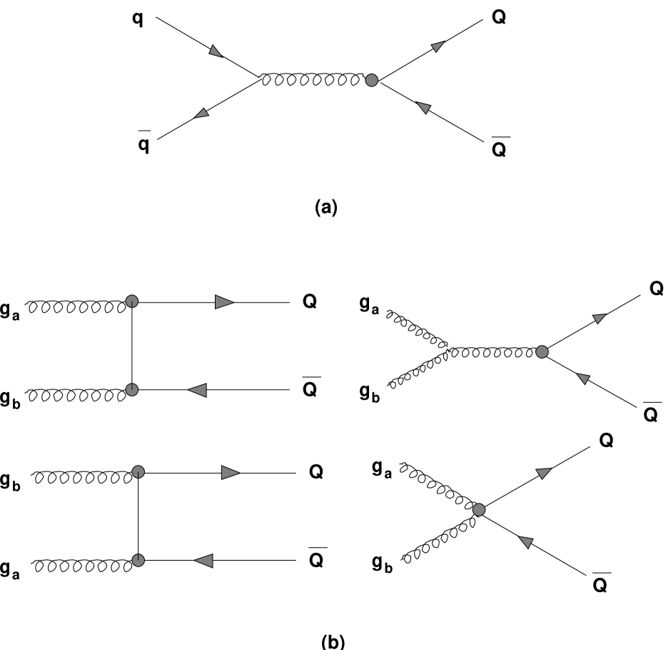
FIG. 1.:

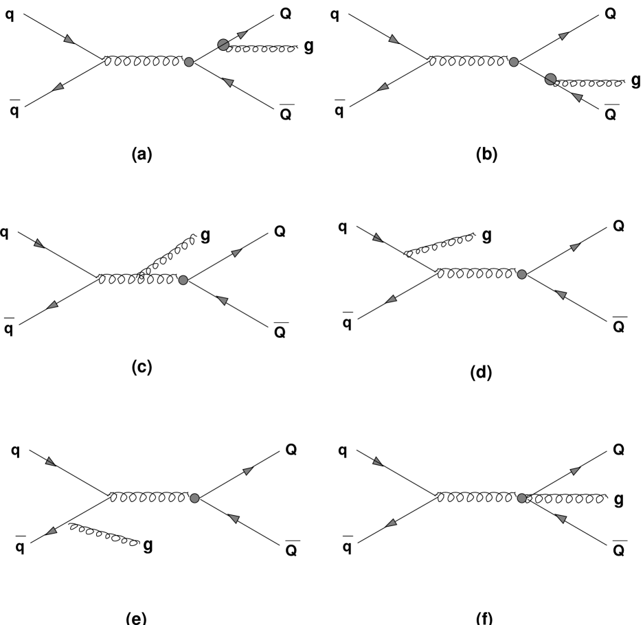
FIG. 2.:

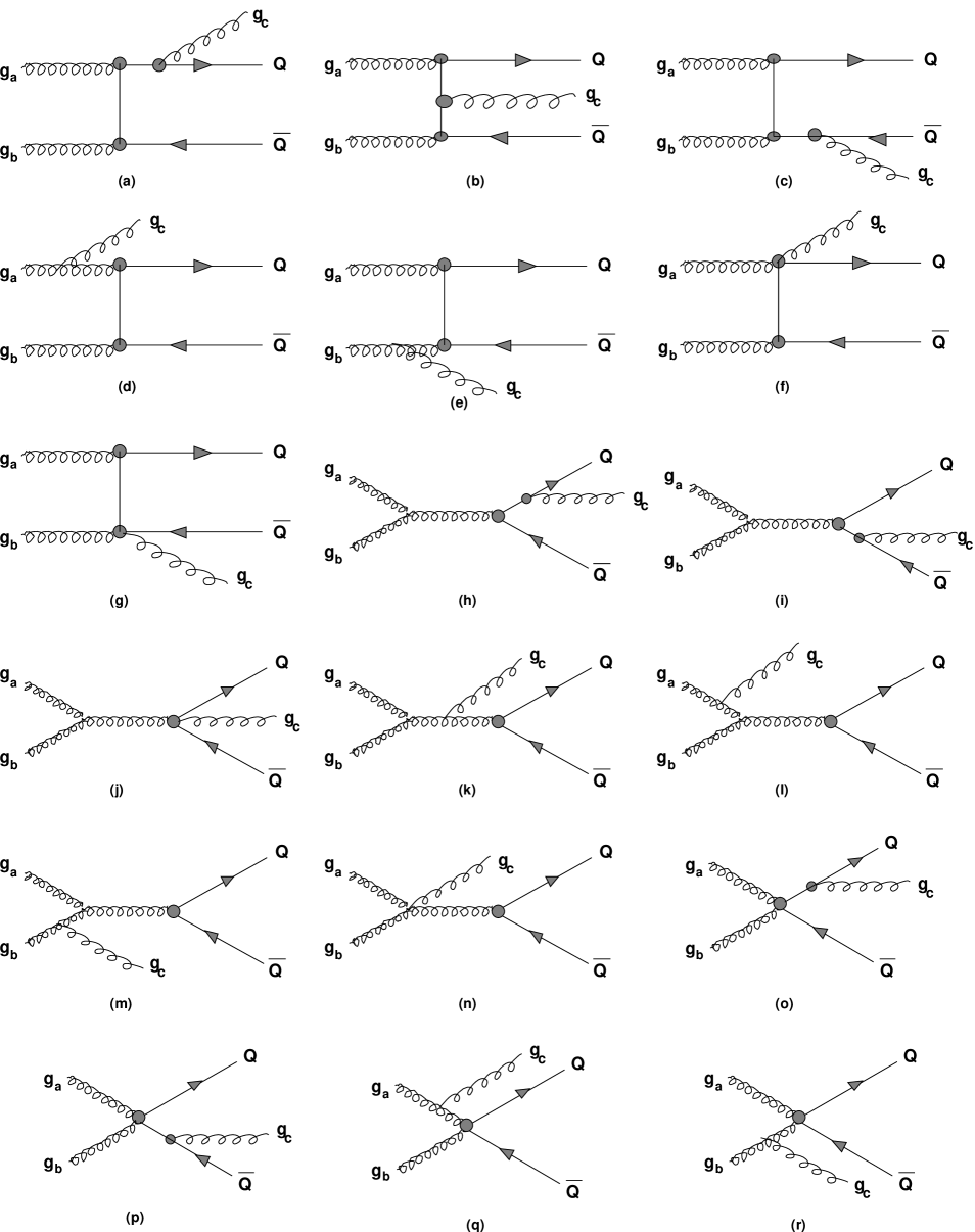
FIG. 3.:

FIG. 4.:

FIG. 5.:

FIG. 6.:

FIG. 7.:

FIG. 8.:

FIG. 9.:

REFERENCES

- [1] F. Abe et al. (CDF Collaboration), Phys. Rev. Lett. 74, 2626 (1995).
- [2] S. Abachi et al. (D0 Collaboration), Phys. Rev. Lett. 74, 2632 (1995).
- [3] S. Willenbrock, talk presented at the International Symposium on Particle Theory and Phenomenology, Iowa State University, hep-ph/9508212 (Aug 1995); T.M. Liss, talk given at the conference EPS95, Brussels, 1995, hep-ph/9510274.
- [4] D. Atwood, A. Aeppli, and A. Soni, Phys. Rev. Lett. 69, 2754 (1992).
- [5] G. Kane, G. Ladinsky, and C.P. Yuan, Phys. Rev. D45, 1531 (1992).
- [6] A. Brandenburg and J.P. Ma, Phys. Lett. B298, 211 (1993).
- [7] D. Atwood, A. Kagan, and T.G. Rizzo, Phys. Rev. D52, 6264 (1995); T.G. Rizzo, SLAC-PUB-95-6758, hep-ph/9506351 (Jun 1995).
- [8] P. Haberl, O. Nachtmann, and A. Wilch, HD-THEP-95-25, hep-ph/9505409 (May 1995).
- [9] B. Grzadkowski and J. Gunion, Phys. Lett. B287, 237 (1992).
- [10] K. Cheung, CPP-95-10, hep-ph/9507411 (Jul 1995).
- [11] S. Weinberg, Phys. Rev. Lett. 37, 657 (1976); Phys. Rev. Lett. 63, 2333 (1989); Phys. Rev. D42, 860 (1990).
- [12] D. Chang, W.-Y. Keung, and I. Phillips, Nucl. Phys. B408, 286 (1993); ERRATUM-ibid. B429, 255 (1994).
- [13] V. Barger, A Stange, and R.J.N. Phillips, Phys. Rev. D44, 1987 (1991).
- [14] T. Stelzer and W.F. Long, Comput. Phys. Commun. 81, 357, (1994).
- [15] R.K. Ellis and J.C. Sexton, Nucl. Phys. B282, 642 (1987).
- [16] H.L. Lai et al. (CTEQ Collaboration), Phys. Rev. D51, 4763 (1995).
- [17] Particle Data Group, Phys. Rev. D50, 1173 (1994).
- [18] I. Bigi et al., Phys. Lett. B181, 157 (1986).
- [19] C.R. Schmidt and M. Peskin, Phys. Rev. Lett. 69, 410 (1992).