On the QCD perturbative expansion for $e^{+}e^{-}\to$ hadrons

Abstract

We study the perturbative QCD series for the hadronic width of the $Z$ boson. We sum a class of large “$\pi^{2}$ terms” and reorganize the series so as to minimize “renormalon” effects. We also consider the renormalization scheme-scale ambiguity of the perturbative results. We find that, with three nontrivial known terms in the perturbative expansion, the treatment of the $\pi^{2}$ terms is quite important, while renormalon effects are less important. The measured hadronic width of the $Z$ is often used to determine the value of $\alpha_{s}(M_{Z}^{2})$. A standard method is to use the perturbative expansion for the width truncated at order $\alpha_{s}^{3}$ in the $\overline{\rm MS}$ scheme with scale $\mu=M_{Z}$. We estimate that the determined value of $\alpha_{s}(M_{Z}^{2})$ should be increased by 0.6% compared to the value extracted with this standard method. After this adjustment for $\pi^{2}$ and renormalon effects, we estimate that the uncertainty in $\alpha_{s}(M_{Z}^{2})$ arising from QCD theory is about $0.4\%$. This is, of course, much less than the experimental uncertainty of about 5%.

I Introduction

The width for $Z\to{\rm hadrons}$ is conventionally described by the ratio $R$ of this width to the width for $Z\to e^{+}e^{-}$. The $Z$ boson need not be on-shell: for theoretical purposes, we can consider $R$ as a function $R(s)$ of the c.m. energy $s$ of the $e^{+}e^{-}$ annihilation that produces the $Z$. Then the measured $R$ is $R(M_{Z}^{2})$. One way of measuring the strong coupling $\alpha_{s}$ is to compare theory and experiment for $R(M_{Z}^{2})$. The purpose of this paper is to discuss some aspects of the theoretical evaluation of $R(s)$: the effect of “$\pi^{2}$ terms” and “renormalons” on the determination of $R$ from the calculated terms in its perturbative expansion in powers of $\alpha_{s}$. Our goal is to suggest ways of evaluating $R(s)$ as precisely as possible from the knowledge of the first three terms in its perturbative expansion and then to estimate the theoretical error in this evaluation. We pose the question of whether $\alpha_{s}(M_{Z}^{2})$ could be extracted at a precision of a few parts per mill from $R(M_{Z}^{2})$ in the hypothetical case that infinitely accurate data were available and uncertainties in the electroweak part of the calculation were zero.

We will conclude that a QCD theoretical error on $\alpha_{s}(M_{Z}^{2})$ of about four parts per mill is possible if one understands this as a one $\sigma$ error estimate: the QCD error is probably about this size. An estimate of the QCD theoretical error at the 95% confidence level would be quite a lot larger because it should include the possibility that certain hypotheses – guesses really – about the behavior of the perturbative expansion are simply wrong. We will try to make clear the nature of the required hypotheses and let the reader form his or her own judgment.

In this paper, we adopt a simplified theoretical framework so that we can concentrate on the QCD effects. We consider $Z\to{\rm hadrons}$ at the Born level in the electroweak interactions. We take the $u$, $d$, $s$, $c$ and $b$ quarks to be exactly massless. We include contributions from virtual top quarks that behave like $\log^{n}(m_{t}^{2}/M_{Z}^{2})$, dropping terms that behave like $(M_{Z}^{2}/m_{t}^{2})^{n}$ as $m_{t}\to\infty$.

Given this theoretical framework, the theoretical expression for $R(M_{Z}^{2})$ has the form

$$R(M_{Z}^{2})=R_{0}\left\{1+{\cal R}(M_{Z}^{2})\right\}.$$ (1)

Here $R_{0}$ is the value of $R$ in the parton model, without perturbative QCD corrections. The QCD corrections are contained in ${\cal R}(M_{Z}^{2})=\alpha_{s}(M_{Z}^{2})/\pi+{\cal O}(\alpha_{s}^{2})$, which is often denoted $\delta_{\rm QCD}$. We study ${\cal R}(M_{Z}^{2})$ and try to estimate the theoretical uncertainty in ${\cal R}(M_{Z}^{2})$ caused by evaluating it in perturbation theory truncated at order $\alpha_{s}^{3}$. For this purpose, we use a nominal value $\overline{\alpha}_{s}(M_{Z}^{2})=0.120$ of the $\overline{\rm MS}$ strong coupling evaluated at $M_{Z}$. If an experimental value for ${\cal R}(M_{Z}^{2})$ were used to extract $\overline{\alpha}_{s}(M_{Z}^{2})$, then the fractional theoretical uncertainty in ${\cal R}(M_{Z}^{2})$ would translate into a fractional uncertainty of the same size for $\alpha_{s}(M_{Z}^{2})$.

When we present numerical results, we choose $M_{Z}=91.188{\ \rm GeV}$ and $\sin^{2}\theta_{W}=0.2319$. We take the top quark pole mass to be 170 GeV, as estimated in Ref. [1] from the CDF and D0 results [2].

The scope of this paper is limited, and in fact we do not attempt to evaluate ${\cal R}(M_{Z}^{2})$ at the level of precision that we are discussing. Such an evaluation involves careful consideration of a large number of small effects. Among these are electroweak effects beyond the Born level [3], effects of non-zero masses for the light quarks [4] and $(M_{Z}^{2}/m_{t}^{2})^{n}$ contributions from virtual loops containing the top quark [5]. We review the status of some of these issues in the appendix to this paper.

II The running coupling and top mass

In this paper we denote by $\alpha_{s}(s)$ the running coupling in a renormalization scheme that may or may not be the $\overline{\rm MS}$ scheme [6]. We denote by $\overline{\alpha}_{s}(s)$ the running coupling as defined by the $\overline{\rm MS}$ scheme with five flavors of light quarks.

The dependence of $\alpha_{s}(se^{t})$ on $t$ is given by the renormalization group equation

$${d\over dt}\left(\pi\over\alpha_{s}(se^{t})\right) = -{\pi^{2}\over\alpha_{s}^{2}(se^{t})}\ \beta(\alpha_{s}(se^{t}))$$ (2)

$$= \beta_{0}+\beta_{1}\ {\alpha_{s}(se^{t})\over\pi}+\beta_{2}\left(\alpha_{s}(se^{t})\over\pi\right)^{2}+\cdots.$$ (3)

We use this equation to derive an approximation for ${\pi/\alpha_{s}(se^{t})}$. We find

$${\pi\over\alpha_{s}(se^{t})} = {\pi\over\alpha_{s}(s)}\,(1+x)+{\beta_{1}\over\beta_{0}}\log(1+x)$$ (6)

$$+{\alpha_{s}(s)\over\pi}\left({\beta_{0}\beta_{2}-\beta_{1}^{2}\over\beta_{0}^{2}}\ {x\over 1+x}+{\beta_{1}^{2}\over\beta_{0}^{2}}\ {\log(1+x)\over 1+x}\right)$$

$$+\cdots,$$

where

$$x=\beta_{0}t\,{\alpha_{s}(s)\over\pi}.$$ (7)

Further terms in this series involve higher powers of $\alpha_{s}(s)/\pi$ times functions of $x$ that are proportional to $x$ for small $x$. We do not include any more terms because the next term involves the coefficient $\beta_{3}$, which is unknown. If we wanted to recover the ordinary perturbative expansion of ${\pi/\alpha_{s}(se^{t})}$ up to order $\alpha_{s}(s)^{2}$, we would note that $x$ is proportional to $\alpha_{s}$ and expand in powers of $x$, then omit terms beyond $x^{2}$ or $x\alpha_{s}$. Eq. (6) is better than the purely perturbative expansion because it is a valid expansion in powers of $\alpha_{s}(s)$ when $x$ is fixed at some finite value. Thus it is useful when $\beta_{0}t$ is as large as $\pi/\alpha_{s}(s)$.

We shall sometimes want to examine the dependence of the results of calculations on the renormalization scheme used in the calculation (Cf. Ref. [7]). For this purpose, we define an $\alpha_{s}$ in a renormalization scheme that may not be the $\overline{\rm MS}$ scheme by

$$\alpha_{s}(s)=\overline{\alpha}_{s}(s)+c_{2}\,\overline{\alpha}_{s}(s)^{2}+c_{3}\,\overline{\alpha}_{s}(s)^{3}+\cdots.$$ (8)

Then one can use $\alpha_{s}(s)$ as the expansion parameter of the theory. Since the perturbative formulas used are inevitably truncated at some order of perturbation theory, the results depend on the coefficients $c_{i}$ that specify the scheme. We will want to find out how much the results depend on the $c_{i}$. There are two purposes to this. First, the choice of renormalization scheme represents an ambiguity of the theory, and we want to have an estimate of the numerical importance of this ambiguity. Second, there are uncalculated higher order terms that are, by necessity, omitted from the calculation. Parts of these terms serve to cancel the dependence of the results on the $c_{i}$. Thus the observed size of the dependence of the result on the $c_{i}$ serves as a rough indicator of the size of the uncalculated higher order terms.

The coefficient $c_{2}$ can be simply absorbed into a change of the scale of the running coupling:

$$\alpha_{s}(s)=\overline{\alpha}_{s}(se^{\delta t})+c_{3}^{\prime}\,\overline{\alpha}_{s}^{3}(se^{\delta t})+\cdots.$$ (9)

That is, using Eq. (6) on the right hand side of Eq. (9) reproduces Eq. (8). The term in Eq. (9) proportional to $\overline{\alpha}_{s}^{3}$ results in a change of the coefficient $\beta_{2}$ in the $\beta$ function that describes the running of $\alpha_{s}$. (Recall that $\beta_{0}$ and $\beta_{1}$ are scheme independent.) Let us parameterize this change as

$$\beta_{2}=\overline{\beta}_{2}+\delta\beta_{2}\,,$$ (10)

where $\overline{\beta}_{2}$ is the third coefficient of the $\beta$ function in the $\overline{\rm MS}$ scheme and other MS-type schemes. Then the relation between $\alpha_{s}$ and $\overline{\alpha}_{s}$ can be written as

$${\alpha_{s}(s)\over\pi}={\overline{\alpha}_{s}(se^{\delta t})\over\pi}+{\delta\beta_{2}\over\beta_{0}}\,\left(\overline{\alpha}_{s}(se^{\delta t})\over\pi\right)^{3}+\cdots.$$ (11)

We shall use $\delta t$ and $\delta\beta_{2}$ to parameterize the choice of scheme.

By combining Eq. (6) with Eq. (11), we see that $\alpha_{s}(s)$ can be expanded in terms of $\overline{\alpha}_{s}(s)$ by using

$${\pi\over\alpha_{s}(s)} = {\pi\over\overline{\alpha}_{s}(s)}\,(1+\delta x)+{\beta_{1}\over\beta_{0}}\log(1+\delta x)$$ (14)

$$+{\overline{\alpha}_{s}(s)\over\pi}\left({\beta_{0}\overline{\beta}_{2}-\beta_{1}^{2}\over\beta_{0}^{2}}\ {\delta x\over 1+\delta x}+{\beta_{1}^{2}\over\beta_{0}^{2}}\ {\log(1+\delta x)\over 1+\delta x}-{\delta\beta_{2}\over\beta_{0}}{1\over 1+\delta x}\right)$$

$$+\cdots.$$

Here,

$$\delta x=\beta_{0}\,\delta t\,{\overline{\alpha}_{s}(s)\over\pi}.$$ (15)

In the framework of this paper (except for the appendix), light quark masses do not appear in $R(s)$ because they are set to zero. However, the top quark mass does appear, starting at order $\alpha_{s}^{2}$. Thus it is necessary to state carefully how we define $m_{t}$. We let $\overline{m}_{t}(s)$ be the running top quark mass within the $\overline{\rm MS}$ scheme. At the level of perturbation theory at which we work, we need the one loop evolution of $\overline{m}_{t}(s)$, which we write as

$$\overline{m}_{t}^{2}(s)\approx\overline{m}_{t}^{2}(M_{Z}^{2})\ \exp\!\left(2\gamma_{0}\int^{s}_{M_{Z}^{2}}{d\mu^{2}\over\mu^{2}}\ {\overline{\alpha}_{s}(\mu^{2})\over\pi}\right)\approx m_{t}^{2}(M_{Z}^{2})\ \left({\overline{\alpha}_{s}(M_{Z}^{2})\over\overline{\alpha}_{s}(s)}\right)^{2\gamma_{0}/\beta_{0}}$$ (16)

with

$$\gamma_{0}=-1.$$ (17)

(See, for instance, Ref. [8]). One can, of course, use a different scheme and define a running mass

$$m_{t}^{2}(s)=\overline{m}_{t}^{2}(s)\,[1+C_{1}\overline{\alpha}_{s}(s)+\cdots].$$ (18)

We do so, absorbing the first coefficient $C_{1}$ into a change of scale by an amount $\delta t_{m}$. Thus we define

$$m_{t}^{2}(s)\approx\overline{m}_{t}^{2}(s)\ \left({\overline{\alpha}_{s}(s)\over\overline{\alpha}_{s}(se^{\delta t_{m}})}\right)^{2\gamma_{0}/\beta_{0}}.$$ (19)

The parameter $\delta t_{m}$ can be chosen independently from the scaling parameter $\delta t$ in the definition (11) of the coupling.

The dependence of ${\cal R}(s)$ on the top quark mass is quite small, so the dependence of ${\cal R}(s)$ on $\delta t_{m}$ is also small. In fact, we find that ${\cal R}(M_{Z}^{2})$ varies by only 0.3 parts per mill for $-4<\delta t_{m}<4$. In order to limit the parameter space to be explored in our numerical examples, we therefore set

$$\delta t_{m}=0.$$ (20)

Thus the running top mass at $s=M_{Z}^{2}$ in our examples is simply the $\overline{\rm MS}$ running top mass $\overline{m}_{t}(M_{Z}^{2})$. We take $\overline{m}_{t}(M_{Z}^{2})=170.2{\ \rm GeV}$, which corresponds to a pole mass of $\tilde{m}_{t}=170{\ \rm GeV}$ after use of

$$\overline{m}_{t}^{2}(M_{Z}^{2})\approx\tilde{m}_{t}^{2}\ \exp\!\left(-{8\over 3}\,{\overline{\alpha}_{s}(\tilde{m}_{t}^{2})\over\pi}\right)\left({\overline{\alpha}_{s}(\tilde{m}_{t}^{2})\over\overline{\alpha}_{s}(M_{Z}^{2})}\right)^{2\gamma_{0}/\beta_{0}}.$$ (21)

(See, for instance, Ref. [8]). The value 170 GeV is estimated in Ref. [1] from the CDF and D0 results [2].

III Perturbative expansions

With the theoretical framework defined in Sec. I, the theoretical expression for $R(s)$ has the form

$$R(s)=R_{0}\left\{1+{\cal R}(s)\right\}.$$ (22)

Here $R_{0}$ is the value of $R(s)$ in the parton model, without perturbative QCD corrections. The QCD corrections are contained in ${\cal R}(s)$,

$${\cal R}(s)={\cal R}_{1}\ {\alpha_{s}(s)\over\pi}+{\cal R}_{2}\left(\alpha_{s}(s)\over\pi\right)^{2}+{\cal R}_{3}\left(\alpha_{s}(s)\over\pi\right)^{3}+\cdots.$$ (23)

The value of ${\cal R}(s)$ calculated in finite order perturbation theory depends on the parameters $\delta t$, $\delta\beta_{2}$ and $\delta t_{m}$ that define the renormalization scheme. We keep these parameters arbitrary in this analysis in order to be able to test the sensitivity of the calculated value of ${\cal R}(s)$ to their choice. As already noted, the dependence of ${\cal R}(s)$ on $\delta t_{m}$ is negligible.

The $t$ dependence of $\alpha_{s}(se^{t})$ is given by the renormalization group equation (3). The coefficients of the $\beta$ function that appears in this equation are [9]

$$\beta_{0} = (33-2\,N_{f})/12,$$ (24)

$$\beta_{1} = (306-38\,N_{f})/48,$$ (25)

$$\beta_{2} = (77139-15099\,N_{f}+325\,N_{f}^{2})/3456+\delta\beta_{2}\,,$$ (26)

where $N_{f}=5$ is the number of light quark flavors used throughout this paper.

The coefficients ${\cal R}_{1},{\cal R}_{2},{\cal R}_{3}$ are [10, 11]

$${\cal R}_{1} = 1,$$ (27)

$${\cal R}_{2} = {365\over 24}-11\,\zeta(3)-N_{f}\left[{11\over 12}-{2\,\zeta(3)\over 3}\right]-{1\over\sum_{i}(v_{i}^{2}+a_{i}^{2})}\ \left[{37\over 12}+\log\!\left(m_{t}(s)^{2}\over M_{Z}^{2}\right)\right]$$ (29)

$$+\beta_{0}\,\delta t,$$

$${\cal R}_{3} = {87029\over 288}-{1103\,\zeta(3)\over 4}+{275\,\zeta(5)\over 6}-{\beta_{0}^{2}\pi^{2}\over 3}$$ (34)

$$+N_{f}\left[-{7847\over 216}+{262\,\zeta(3)\over 9}-{25\,\zeta(5)\over 9}\right]+N_{f}^{2}\left[{151\over 162}-{19\,\zeta(3)\over 27}\right]$$

$$+{\left(\sum_{i}v_{i}\right)^{2}\over\sum_{i}(v_{i}^{2}+a_{i}^{2})}\left[{55\over 72}-{5\,\zeta(3)\over 3}\right]$$

$$+{1\over\sum_{i}(v_{i}^{2}+a_{i}^{2})}\left[-18.65440-{31\over 18}\,\log\!\left(m_{t}(s)^{2}\over M_{Z}^{2}\right)+{23\over 12}\,\log^{2}\!\left(m_{t}(s)^{2}\over M_{Z}^{2}\right)+2\gamma_{0}\,\delta t_{m}\right]$$

$$+\beta_{0}^{2}\,(\delta t)^{2}+\left[\beta_{1}+2\beta_{0}{\cal R}_{2,0}\right]\,\delta t-{\delta\beta_{2}\over\beta_{0}}.$$

Here $(v_{i},a_{i})$ with $i=u,d,s,c,b$ is the (vector, axial vector) coupling of the quark of flavor $i$ to the $Z$ boson, as specified in the appendix. We use ${\cal R}_{2,0}$ to denote ${\cal R}_{2}$ with $\delta t=0$. We recall that the mass anomalous dimension is $\gamma_{0}=-1$ and that the parameters $\delta t$, $\delta\beta_{2}$ and $\delta t_{m}$ give the scheme dependence, as described in Sec. II.

The numerical values are

$$\beta_{0} \approx 1.92,$$ (35)

$$\beta_{1} \approx 2.42,$$ (36)

$$\beta_{2} \approx 2.83+\delta\beta_{2},$$ (37)

and (with $\delta t_{m}=0$ and $m_{t}(s)=\overline{m}_{t}(M_{Z}^{2})$)

$${\cal R}_{1} = 1,$$ (38)

$${\cal R}_{2} \approx 0.76+1.92\,\delta t,$$ (39)

$${\cal R}_{3} \approx -15.73+5.35\,\delta t+3.67\,(\delta t)^{2}-0.52\,\delta\beta_{2}.$$ (40)

In this paper, we will define various approximations ${\cal R}_{A}$ to ${\cal R}$. The first of these is the simple third order perturbative approximation:

$${\cal R}_{A}(s;{\rm Pert})=\sum_{j=1}^{3}{\cal R}_{j}\left(\alpha_{s}(s)\over\pi\right)^{j}.$$ (41)

As discussed in Sec. II, the renormalization scheme ambiguity can provide an estimate, or at least a lower bound, on the theoretical uncertainty produced by truncating perturbation theory at order $\alpha_{s}^{3}$. To investigate this ambiguity, we show in Fig. 1 a contour plot of ${\cal R}_{A}(M_{Z}^{2};{\rm Pert})$ as a function of $\delta t$ and $\delta\beta_{2}$, with $\delta t_{m}=0$. The range shown for the scale parameter, $-4<\delta t<4$, corresponds to scales $\mu=[se^{t}]^{1/2}$ in the range $0.14\,M_{Z}\approx M_{Z}e^{-2}<\mu<M_{Z}e^{2}\approx 7.4\,M_{Z}$ in Eq. (11). The range shown for $\delta\beta_{2}$ corresponds to schemes with $-1.2\approx\overline{\beta}_{2}-4<\beta_{2}<\overline{\beta}_{2}+4\approx 6.8$.

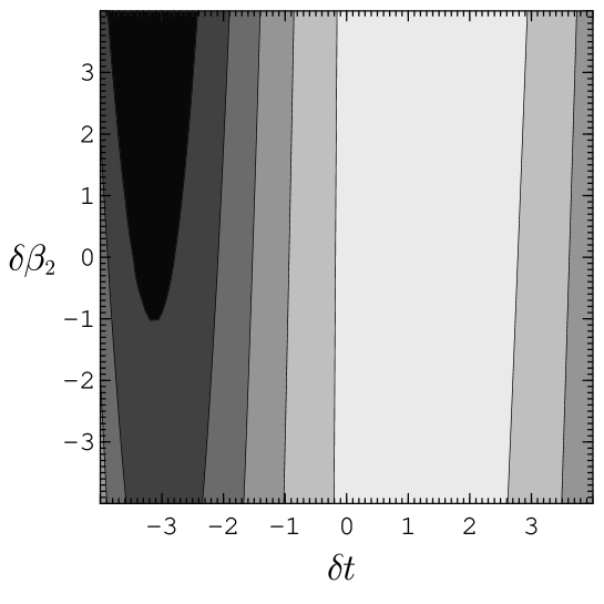
FIG. 1.: Contour plot of the simple third order perturbative approximant ${\cal R}_{A}(M_{Z}^{2};{\rm Pert})$, Eq. (41), versus the scheme fixing parameters $\delta t$ and $\delta\beta_{2}$, with $\delta t_{m}=0$.

We learn from Fig. 1 that ${\cal R}_{A}(M_{Z}^{2};{\rm Pert})$ is not very sensitive to $\delta\beta_{2}$. Accordingly, we set $\delta\beta_{2}=0$ and plot ${\cal R}_{A}(M_{Z}^{2};{\rm Pert})$ versus $\delta t$ in Fig. 2. We note that ${\cal R}_{A}(M_{Z}^{2};{\rm Pert})$ varies by about 2.6% between its local maximum and its local minimum. We conclude that ${\cal R}(M_{Z}^{2})$ probably lies within this 2.6% range. Thus we ascribe a theoretical error of $\pm 2.6\%/2=\pm 1.3\%$ to the value of ${\cal R}(M_{Z}^{2})$. In the remainder of this paper, we attempt to reduce this error by using more sophisticated methods than simply taking the first three perturbative terms in ${\cal R}(M_{Z}^{2})$.

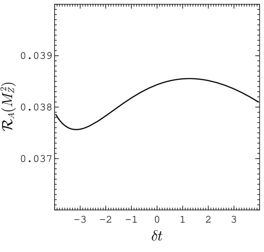
FIG. 2.: Plot of the usual third order perturbative approximant ${\cal R}_{A}(M_{Z}^{2};{\rm Pert})$ versus the scheme fixing parameter $\delta t$ with $\delta\beta_{2}=0$ and $\delta t_{m}=0$.

The perturbative series for ${\cal R}(M_{Z}^{2})$ provides our starting point. We see that the series for $\beta(\alpha_{s})$ is nicely behaved, but that the series for ${\cal R}(s)$ not as well behaved, with a large value for ${\cal R}_{3}$ at $\delta t=\delta\beta_{2}=\delta t_{m}=0$. In fact, this large value can be attributed to the term $-\beta_{0}^{2}\pi^{2}/3\approx-12.1$.

IV $\pi^{2}$ terms

The offending $\pi^{2}$ term in ${\cal R}_{3}$ arises, at a rather mechanical calculational level, because factors of $\log(-s\pm i\epsilon)=\log(s)\pm i\pi$ occur in the calculation, leading to powers of $\pi$ in the result. In order to see what happens at higher orders of perturbation theory, we write $R(s)$ as a discontinuity:

$$R(s)={C\over 2\pi i}\left\{\Pi(-s+i\epsilon,\mu^{2})-\Pi(-s-i\epsilon,\mu^{2})\right\}.$$ (42)

Here $C$ is a normalization constant and $\Pi(Q^{2},\mu^{2})$ is the standard $Z$ boson self-energy function including the QCD contribution. It is proportional to the Fourier transform of the time ordered product of two weak current operators. The current operators carry momentum $q^{\mu}$. We define $Q^{2}=-q^{\mu}q_{\mu}$, so that $Q^{2}>0$ if the momentum $q^{\mu}$ is spacelike. The function $\Pi$ depends on the renormalization scale $\mu^{2}$. However the function

$$D(Q^{2})=-Q^{2}{\partial\over\partial Q^{2}}\Pi(Q^{2},\mu^{2})$$ (43)

is a renormalization group invariant. The derivative here avoids the overall renormalization in $\Pi$. For this reason, it is standard practice to work with $D(Q^{2})$.

We may write the perturbative expansion of $D(Q^{2})$ in the form

$$D(Q^{2})=D_{0}\left\{1+{\cal D}(Q^{2})\right\},$$ (44)

where $D_{0}$ is the value of $D$ in the parton model and where

$${\cal D}(Q^{2})={\cal D}_{1}\ {\alpha_{s}(Q^{2})\over\pi}+{\cal D}_{2}\left(\alpha_{s}(Q^{2})\over\pi\right)^{2}+{\cal D}_{3}\left(\alpha_{s}(Q^{2})\over\pi\right)^{3}+\cdots.$$ (45)

The first three coefficients ${\cal D}_{n}$ are the same as the corresponding ${\cal R}_{n}$ in Eq. (29) if one substitutes $Q^{2}$ for $s$, except that ${\cal D}_{3}$ lacks the term $-\beta_{0}^{2}\pi^{2}/3$. The numerical values (with $\delta t_{m}=0$ and $m_{t}(s)=\overline{m}_{t}(M_{Z}^{2})$) are

$${\cal D}_{1} = 1,$$ (46)

$${\cal D}_{2} \approx 0.76+1.92\,\delta t,$$ (47)

$${\cal D}_{3} \approx -3.65+5.35\,\delta t+3.67\,(\delta t)^{2}-0.52\,\delta\beta_{2}.$$ (48)

If we stay near $\delta t=0$, this series appears to be quite nicely behaved. We believe on the basis of general arguments (to be discussed in the next section) that the coefficients ${\cal D}_{n}$ will eventually grow for large $n$. However, that growth is not apparent in the first three terms.

The function $D(Q^{2})$ is calculated using Euclidean quantum field theory, in which only very weak infrared singularities occur near the contour of the internal momentum integrations. On the other hand, a direct calculation of $R(s)$ involves Minkowski momentum integrations over regions in which various internal particles can go on shell. Only some delicate cancellations prevent $R(s)$ from being infinite. Surely $D(Q^{2})$ should be better behaved than $R(s)$. This observation leads to the following

Hypothesis 1. The perturbative expansion of $D(Q^{2})$ remains well behaved beyond the three terms that are known, subject only to the eventual growth of the ${\cal D}_{n}$ dictated by the standard renormalon and instanton ideas.

We adopt this hypothesis here, although it is criticised in Ref. [12] on the grounds that there could be other sources of large perturbative coefficients in ${\cal D}(s)$.

We are interested in the observable function $R(s)$. If we accept this Hypothesis 1, then instead of calculating $R(s)$ directly, we should relate it to the nicely behaved function $D(Q^{2})$. From Eqs. (42) and (43) we obtain

$${\cal R}(s)={1\over 2\pi}\int_{-\pi}^{\pi}d\theta\ {\cal D}(se^{i\theta}).$$ (49)

In the following section, we will deal with the expected large order behavior of the ${\cal D}_{n}$ by following the standard practice of using the Borel transform $\tilde{\cal D}$ of ${\cal D}$:

$${\cal D}(Q^{2})=\int_{0}^{\infty}\!dz\ \exp\!\left(-{\pi z\over\alpha_{s}(Q^{2})}\right)\ \tilde{\cal D}(z).$$ (50)

If we write the perturbative expansion of $\tilde{\cal D}(z)$ as

$$\tilde{\cal D}(z)=\tilde{\cal D}_{0}+\tilde{\cal D}_{1}\ z+\tilde{\cal D}_{2}\ z^{2}+\cdots,$$ (51)

then

$$\tilde{\cal D}_{n}={{\cal D}_{n+1}\over n!}.$$ (52)

Because of the $1/n!$ factor, the perturbative expansion of $\tilde{\cal D}$ in powers of $z$ is much nicer than that of $\tilde{\cal D}$ in powers of $\alpha_{s}/\pi$. In fact, one expects $\tilde{\cal D}(z)$ to be analytic near $z=0$. As discussed, for example, in Ref. [13], there are singularities expected in the complex $z$ plane, including some on the integration contour along the positive $z$-axis. In addition $\tilde{\cal D}(z)$ is not expected to be well behaved as $z\to\infty$. Thus the meaning of the integration in Eq. (50) is ambiguous. In this section, we simply leave it as ambiguous.

We can relate ${\cal R}(s)$ to $\tilde{\cal D}$ by inserting Eq. (50) into Eq. (49):

$${\cal R}(s)=\int_{0}^{\infty}\!dz\ \exp\!\left(-{\pi z\over\alpha_{s}(s)}\right)\ F(\alpha_{s}(s),z)\ \tilde{\cal D}(z),$$ (53)

where

$$F(\alpha_{s},z)={1\over 2\pi}\int_{-\pi}^{\pi}d\theta\ \exp\!\left(-zG(\alpha_{s},\theta)\right),$$ (54)

with

$$G(\alpha_{s}(s),\theta)={\pi\over\alpha_{s}(se^{i\theta})}-{\pi\over\alpha_{s}(s)}.$$ (55)

Eq. (53) is the basis for the analysis in this paper. We note that the factor $\pi/\alpha_{s}(s)$ in the exponent in Eq. (53) is big, about 30 for $\alpha_{s}\approx 0.12$. Therefore the integral over $z$ is dominated by small $z$, $\beta_{0}z\lesssim\beta_{0}\alpha_{s}/\pi\approx 0.06$. Thus we will be primarily concerned with the expansion of $\tilde{\cal D}(z)$ in powers of $z$.

Before addressing $\tilde{\cal D}(z)$, however, we need a good approximation for $F(\alpha_{s},z)$. Since small $z$ is important, we are particularly interested in the small $z$ region. However, it is rather easy to find an approximation for $F(\alpha_{s},z)$ that is good for a wide range of $z$, based on the smallness of its argument $\alpha_{s}$. We use the solution (6) of the renormalization group equation (3) for $\pi/\alpha_{s}$ in order to derive an approximation for $G(\alpha_{s},\theta)$. We find $G(\alpha_{s},\theta)\approx G_{A}(\alpha_{s},\theta)$ where

$$G_{A}(\alpha_{s},\theta) = i\beta_{0}\theta+{\beta_{1}\over\beta_{0}}\log(1+y)$$ (57)

$$+{\alpha_{s}\over\pi}\left({\beta_{0}\beta_{2}-\beta_{1}^{2}\over\beta_{0}^{2}}\ {y\over 1+y}+{\beta_{1}^{2}\over\beta_{0}^{2}}\ {\log(1+y)\over 1+y}\right),$$

where

$$y=i\beta_{0}\theta\,{\alpha_{s}\over\pi}.$$ (58)

Further terms in this series involve higher powers of $\alpha_{s}/\pi$ times functions of $y$ that vanish for $y\to 0$. The ordinary perturbative expansion of $G(s)$ results from expanding in powers of $y$, which is proportional to $\alpha_{s}$, then omitting terms beyond $y^{2}$ or $y\alpha_{s}$. However, $\alpha_{s}(s)/\pi\approx 1/30$ while $|y|\approx 1/5$ at $\theta=\pi$. Thus $\alpha_{s}(s)/\pi$ is a much better expansion parameter than $y$. Since we don’t have to expand in $y$, we don’t.

We now have an approximation $G_{A}(\alpha_{s},\theta)$ for $G(\alpha_{s},\theta)$. Our corresponding approximation $F_{A}(\alpha_{s},z)$ for $F(\alpha_{s},z)$ is

$$F_{A}(\alpha_{s},z)={1\over 2\pi}\int_{-\pi}^{\pi}d\theta\ \exp\!\left(-zG_{A}(\alpha_{s},\theta)\right),$$ (59)

with the integral computed to sufficient accuracy by numerical methods. In Fig. 3 we show a graph of $F_{A}(\alpha_{s},z)$ versus $\beta_{0}z$ superimposed on a graph of $\exp(-\pi z/\alpha_{s})$, all with $\alpha_{s}=0.12$.

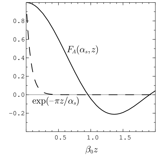
FIG. 3.: Graph of $F_{A}(\alpha_{s},z)$ and $\exp(-\pi z/\alpha_{s})$ versus $\beta_{0}z$ with $\alpha_{s}=0.12$

How good is our approximation $F_{A}(\alpha_{s},z)$? The first omitted term in $G(\alpha_{s},\theta)$ is, in the $\overline{\rm MS}$ scheme,

$$\Delta G(\alpha_{s})=\left(\alpha_{s}\over\pi\right)^{2}h(x),$$ (60)

where

$$h(x) = -{\beta_{1}^{3}\over 2\beta_{0}^{3}}{\log^{2}(1+x)\over(1+x)^{2}}+{\beta_{1}\beta_{2}\over\beta_{0}^{2}}{\log(1+x)\over(1+x)^{2}}$$ (62)

$$+{\beta_{1}^{3}\over 2\beta_{0}^{3}}{x^{2}\over(1+x)^{2}}-{\beta_{1}\beta_{2}\over\beta_{0}^{2}}{x\over(1+x)}+{\beta_{3}\over 2\beta_{0}}{x(x+2)\over(1+x)^{2}}.$$

This term contains a factor $(\alpha_{s}/\pi)^{2}\approx 10^{-3}$ for $\alpha_{s}\approx 0.1$. This factor multiplies $h(x)$, which cannot be evaluated because it contains the unknown coefficient $\beta_{3}$. However, we can see from the structure of $h(x)$ that it is not large unless $\beta_{3}$ is large. We can get a quantitative idea of the effect of $\Delta G$ by choosing some plausible values for $\beta_{3}$ and then calculating ${\cal R}(s)$ with $\Delta G$ included. We find that, taking $\beta_{3}$ in the range $-10<\beta_{3}<10$, the fractional change ${\cal R}(M_{Z}^{2})$ induced by including $\Delta G(\alpha_{s})$ is no larger than $2\times 10^{-5}$. Since this error is small compared to our target error of a few per mill, we can safely neglect it.

We thus obtain an approximation for $\cal R$ that uses third order perturbation theory but sums certain “$\pi^{2}$” effects to all orders:

$${\cal R}_{A}(s;\pi^{2})=\int_{0}^{\infty}\!dz\ \exp\!\left(-{\pi z\over\alpha_{s}(s)}\right)\ F_{A}(\alpha_{s}(s),z)\ \tilde{\cal D}_{A}(z),$$ (63)

where $F_{A}$ is given in Eq. (59) and $\tilde{\cal D}_{A}(z)$ is simply $\tilde{\cal D}(z)$, Eq. (51), expanded to second order in $z$.

This treatment of $\pi^{2}$ terms is similar in spirit to that of Le Diberder and Pich [14], who expand ${\cal D}(se^{i\theta})$ in Eq. (49) in perturbation theory, use Eq. (6) for $\alpha_{s}(se^{i\theta})$, and perform the $\theta$ integral exactly. We simply embed this approach into the Borel transform.

In Fig. 4 we plot ${\cal R}_{A}(M_{Z}^{2};\pi^{2})$ versus the scheme parameter $\delta t$ with the other scheme parameters set to $\delta\beta_{2}=0$ and $\delta t_{m}=0$. We overlay the plot of ${\cal R}_{A}(M_{Z}^{2};{\rm Pert})$ from Fig. 2. We note that ${\cal R}_{A}(M_{Z}^{2};\pi^{2})$ varies by about 0.32% between its local maximum and its local minimum. This is a much smaller variation than that of ${\cal R}_{A}(M_{Z}^{2};{\rm Pert})$. A very optimistic view would be that ${\cal R}(M_{Z}^{2})$ probably lies within this 0.32% range, so that one would ascribe a theoretical error of $\pm 0.32\%/2=\pm 0.16\%$ to the value of ${\cal R}(M_{Z}^{2})$. However, this error estimate is smaller than other error estimates that we will develop later. We therefore regard the flatness of the curve for ${\cal R}_{A}(M_{Z}^{2};\pi^{2})$ as being partially the result of an accidental cancellation, and refrain from taking 0.16% as a reasonable error estimate.

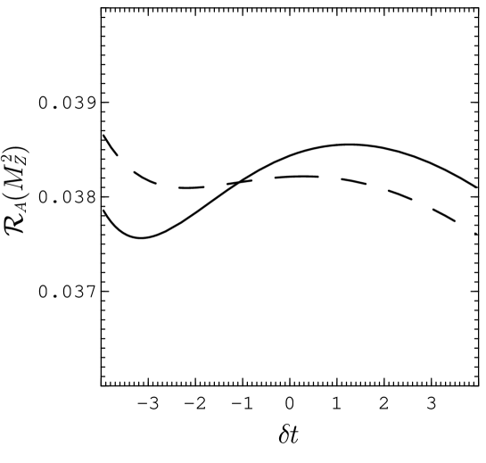
FIG. 4.: Plot of $\pi^{2}$-summed approximant ${\cal R}_{A}(M_{Z}^{2};\pi^{2})$, Eq. (63), (dashed line), versus the scheme fixing parameter $\delta t$ with $\delta\beta_{2}=0$ and $\delta t_{m}=0$. We also show ${\cal R}_{A}(M_{Z}^{2};{\rm Pert})$ from Fig. 2 (full line).

We close this section by emphasizing the observation that the straightforward perturbative expansion of ${\cal R}(s)$ is, in part, an expansion in powers of $\beta_{0}\theta\,[{\alpha_{s}(s)/\pi}]$, with $\theta\sim\pi$, instead of an expansion in powers of $[\alpha_{s}(s)/\pi]\approx 1/30$. One can attribute the appearance of “$\pi^{2}$” terms in ${\cal R}(s)$ to this phenomenon. This observation helps to make Hypothesis 1 plausible. Unfortunately, this argument is only suggestive, since one can not be sure that there are not “bad expansion parameters” lurking somewhere in the calculation of ${\cal D}(Q^{2})$. In the next section, we turn to the behavior of the perturbative coefficients in $\tilde{\cal D}(z)$, assuming that the evidence for a bad expansion parameter is not, in fact, lurking just beyond the last calculated coefficient.

V Truncation of the integral

If we do not expand $\tilde{\cal D}(z)$ in powers of $z$, then at this point we have an approximation for $\cal R$ of the form

$${\cal R}(s)\approx\int_{0}^{\infty}\!dz\ \exp\!\left(-{\pi z\over\alpha_{s}(s)}\right)\ F_{A}(\alpha_{s}(s),z)\ \tilde{\cal D}(z),$$ (64)

with $F_{A}$ given in Eq. (59). Since $\alpha_{s}(s)$ is small, the dominant integration region is $z\ll 1$. Indeed, taking $\alpha_{s}\approx 0.12$, we have $\exp\!\left(-{\pi z/\alpha_{s}}\right)<10^{-3}$ for $\beta_{0}z>0.51$. Thus it is useful to write ${\cal R}$ in the form

$${\cal R}(s)\approx\int_{0}^{z_{\rm max}}\!dz\ \exp\!\left(-{\pi z\over\alpha_{s}(s)}\right)\ F_{A}(\alpha_{s}(s),z)\ \tilde{\cal D}(z)+{\cal R}_{R}(s)$$ (65)

with $\beta_{0}z_{\rm max}\gtrsim 0.5$. The fundamental question of how the “sum of perturbation theory” is precisely defined relates to the definition of ${\cal R}_{R}$. In turn, this question is related to how the renormalon and instanton singularities are treated and to the question of the convergence of the integral at large $z$. However, our purpose here is at once more modest and more practical. We adopt

Hypothesis 2. It is safe to ignore the large $z$ part of the Borel integral when calculating ${\cal R}(s)$ for $s\sim M_{Z}$, even though this part of the integral is ill defined.

We thus neglect ${\cal R}_{R}$ and concentrate on the integral up to $z_{\rm max}$ in Eq. (65). The advantage is that we can use approximations for $\tilde{\cal D}(z)$ that have singularities on the positive $z$ axis outside of the region of integration.

We can test the sensitivity of the computed value of $\cal R$ to $z_{\rm max}$ by replacing $\tilde{\cal D}(z)$ by its second order expansion in powers of $z$. Then the ratio of the two terms in Eq. (65) with $z_{\rm max}=0.5$ (for $s=M_{Z}^{2},\ \delta t=\delta t_{m}=\delta\beta_{3}=0$) is ${\cal R}_{R}(s)/{\cal R}_{A}(s;\pi^{2})\approx 6\times 10^{-4}$.

VI Accounting for renormalons

We now turn to the perturbative expansion

$$\tilde{\cal D}(z)=\sum_{0}^{\infty}\tilde{\cal D}_{n}\,z^{n}.$$ (66)

The coefficients $\tilde{\cal D}_{n}$ can be expressed as an integral,

$$\tilde{\cal D}_{n}={1\over 2\pi i}\int_{\cal C}dz\ z^{-n-1}\tilde{\cal D}(z).$$ (67)

The contour $\cal C$ encloses the point $z=0$ but excludes any singularities of $\tilde{\cal D}(z)$. Thus the behavior of the ${\cal D}_{n}$ at large order $n$ is controlled by the part of the contour that lies nearest to $z=0$, which in turn is controlled by the singularities of $\tilde{\cal D}(z)$ that are nearest to $z=0$. A singularity of the form $(z-z_{0})^{-A}$ makes a contribution to ${\cal D}_{n}$ that is proportional to $z_{0}^{-n}\,n^{A-1}$. Thus the most important determinant of the singularity’s contribution to the $\tilde{\cal D}_{n}$ at large $n$ is its location, $z_{0}$. A small $z_{0}$ produces large coefficients. The next most important determinant is the strength of the singularity, $A$. A large positive value of $A$ produces large coefficients.

The nearest singularities are thought to be the first two ultraviolet renormalon singularities at $\beta_{0}z=-1$ and $-2$ and the first infrared renormalon singularity at $\beta_{0}z=+2$ [13, 15]. In this section, we use the available information on these singularities to obtain a perturbative expansion that has better convergence properties. Of course, “better convergence properties” refers to the perturbative coefficients for large $n$. It is problematical whether convergence improvement helps already after only three terms of the series.

The first ultraviolet renormalon singularity is at $\beta_{0}z=-1$. This is the singularity that is closest to the origin (at least so far as anyone knows). It thus controls the large order behavior of the perturbative series. Unfortunately, the theory of the ultraviolet renormalon singularities is not as simple or as well developed as that for the infrared renormalon singularities. (See, however, Ref. [16]). For instance, the strength of the singularity is not known.

The first infrared renormalon singularity is at $\beta_{0}z=+2$. There are other singularities farther away from the origin along the positive real $z$-axis, but we need not be concerned with them: since they lie farther from $z=0$, their contribution to the large order behavior of the perturbative coefficients is weaker than that of the first singularity. It is significant that there is no infrared renormalon singularity at $\beta_{0}z=+1$. The first infrared renormalon singularity has a power behavior,

$$\tilde{\cal D}(z)\sim c\left[1-{\beta_{0}z\over 2}\right]^{-1-2\beta_{1}/\beta_{0}^{2}},$$ (68)

where $c$ is a constant [13, 15]. Numerically, the exponent is ${-1-2\beta_{1}/\beta_{0}^{2}}\approx-2.3$.

We can make use of this information. Consider the function

$$\tilde{\cal C}(z)=\tilde{\cal D}(z)\left[1-{\beta_{0}z\over 2}\right]^{1+2\beta_{1}/\beta_{0}^{2}}.$$ (69)

The factor multiplying $\tilde{\cal D}(z)$ cancels its divergence as $\beta_{0}z\to 2$. The function $\tilde{\cal C}(z)$ is still singular at $\beta_{0}z=2$, since if we multiply a term in $\tilde{\cal D}(z)$ that is analytic at $\beta_{0}z=2$ by the nonanalytic factor, we create a nonanalytic term. However, singularity is much weaker than it was, behaving like

$$\tilde{\cal C}(z)\sim c\left[1-{\beta_{0}z\over 2}\right]^{1+2\beta_{1}/\beta_{0}^{2}}.$$ (70)

Thus the perturbative expansion of $\tilde{\cal C}(z)$ would be better behaved than that of $\tilde{\cal D}(z)$ at large order if it were not for the fact that the leading ultraviolet renormalon singularity at $\beta_{0}z=-1$ dominates the large order behavior.

We can, however, improve the large order behavior arising from the leading ultraviolet renormalon by merely moving it out of the way by means of a good choice of variable. Following Mueller [15] we define a new variable $\zeta$ by

$$\beta_{0}z={\beta_{0}\zeta\over(1-\beta_{0}\zeta/4)^{2}}\ ,\hskip 28.45274pt\beta_{0}\zeta=4\,{\sqrt{1+\beta_{0}z}-1\over\sqrt{1+\beta_{0}z}+1}.$$ (71)

This transformation maps the origin of the $z$-plane onto the origin of the $\zeta$-plane. We have chosen the normalization of $\zeta$ such that

$$\zeta\sim z+{\cal O}(z^{2}).$$ (72)

near $z=0$. The map treats specially the interval $\beta_{0}z<-1$ on the negative $z$-axis that contains the ultraviolet renormalon singularities. The whole complex $z$-plane except for this interval is mapped to the interior of the disk $|\beta_{0}\zeta|<4$ in the $\zeta$-plane. The singularity-free interval $-1<\beta_{0}z<0$ in the negative $z$-axis is mapped onto the interval $-4<\beta_{0}\zeta<0$ of the negative $\zeta$-axis while the interval $0<\beta_{0}z<\infty$ on the positive $z$-axis, which contains the infrared renormalon and instanton singularities, is mapped into the interval $0<\beta_{0}\zeta<4$ of the positive $\zeta$-axis.

We consider the function

$$\tilde{\cal B}(\zeta)=\tilde{\cal C}(z(\zeta)).$$ (73)

The singularity of $\tilde{\cal B}(\zeta)$ that is nearest to the origin of the $\zeta$-plane is the first infrared renormalon singularity, which is at

$$\beta_{0}\zeta=4{\sqrt{3}-1\over\sqrt{3}+1}\approx 1.1.$$ (74)

Thus moving the ultraviolet renormalon singularity away has had a price. We have moved the infrared renormalon singularity closer to the origin. However, we have previously softened the infrared renormalon singularity, so the price is not too great. The net effect should be an improvement.

The effect of singularity mapping has been investigated recently by Altarelli et al. [12]. However, these authors did not also soften the infrared renormalon singularity. They found that there was no gain in this method.

In order to use the singularity softening and mapping, we use the first three terms in the perturbative expansion of $\tilde{\cal D}(z)$,

$$\tilde{\cal D}(z) = 1+\biggl{[}\,0.40+1.00\,\delta t\biggr{]}\,(\beta_{0}z)$$ (76)

$$\ \ +\ \biggl{[}-0.50+0.73\,\delta t+0.50\,(\delta t)^{2}\biggr{]}\,(\beta_{0}z)^{2}+\cdots,$$

to calculate the first three terms in the perturbative expansion of $\tilde{\cal B}(\zeta)$. The result is

$$\tilde{\cal B}(\zeta) = 1+\biggl{[}-0.76+1.00\,\delta t\biggr{]}\,(\beta_{0}\zeta)$$ (78)

$$\ \ +\ \biggl{[}-0.96+0.07\,\delta t+0.50\,(\delta t)^{2}\biggr{]}\,(\beta_{0}\zeta)^{2}+\cdots.$$

(Here we have displayed the coefficients numerically, with the choices $\delta\beta_{2}=\delta t_{m}=0$ and $m_{t}(s)=\overline{m}_{t}(M_{Z}^{2})$.)

This perturbative series for $\tilde{\cal B}(\zeta)$ is supposed to be better behaved at large orders than was the perturbative series for $\tilde{\cal D}(z)$. The expected improvement is not, however, visible in the first three terms. In fact, we started with a series that was quite well behaved, and we have applied a rather mild improvement program. As long as the infrared and untraviolet renormalon singularities are as described in this section, this program may be expected to make the perturbative coefficients smaller at high order, but one cannot expect too much to happen at order two.

An example of this procedure applied to a simple model may be useful as an illustration of what happens at high order. Suppose that

$$\tilde{\cal D}(z)={z\over\left[1+\beta_{0}z\right]}+{1\over\left[1-\beta_{0}z/2\right]^{p}}$$ (79)

with $p={1+2\beta_{1}/\beta_{0}^{2}}$. Then the perturbative expansion of $\tilde{\cal D}(z)$ is

$$\tilde{\cal D}(z) = 1+1.68\,\beta_{0}z+0.44\,(\beta_{0}z)^{2}+1.21\,(\beta_{0}z)^{3}$$ (81)

$$-0.06\,(\beta_{0}z)^{4}+0.81\,(\beta_{0}z)^{5}-0.35\,(\beta_{0}z)^{6}+\cdots.$$

Applying the renormalon improvement procedure gives the function $\tilde{\cal B}(\zeta)$ with a perturbative expansion

$$\tilde{\cal B}(\zeta) = 1+0.52\,\beta_{0}\zeta-0.87\,(\beta_{0}\zeta)^{2}+0.30\,(\beta_{0}\zeta)^{3}$$ (83)

$$-0.02\,(\beta_{0}\zeta)^{4}+0.06\,(\beta_{0}\zeta)^{5}-0.01\,(\beta_{0}\zeta)^{6}+\cdots.$$

The series for $\tilde{\cal B}$ is clearly better behaved at high orders than the series for $\tilde{\cal D}$ . One might claim to see an improvement beginning with the fourth term, which corresponds to the first uncalculated term in the case of the real $\tilde{\cal D}$ and $\tilde{\cal B}$ functions. However, at this quite low order of expansion, the improvement is marginal.

The procedure for singularity softening and mapping may be summarized as follows. We calculate the first $N$ terms in the expansion of $\tilde{\cal B}(\zeta)$ according to Eqs. (69) and (73), where for us $N=3$. Then we instead of using

$$\tilde{\cal D}_{A}(z)\equiv\sum_{n=0}^{2}\tilde{\cal D}_{n}z^{n}$$ (84)

for $\tilde{\cal D}(z)$ in Eq. (65), we use

$$\tilde{\cal D}_{A^{\prime}}(z)\equiv\left[1-{\beta_{0}z\over 2}\right]^{-1-2\beta_{1}/\beta_{0}^{2}}\,\sum_{n=0}^{2}\tilde{\cal B}_{n}\ \left[\zeta(z)\right]^{n}.$$ (85)

This gives an approximation for ${\cal R}(s)$ that we may call ${\cal R}_{A}(s;\pi^{2},{\rm R\hbox{'}lons})$:

$${\cal R}_{A}(s;\pi^{2},{\rm R\hbox{'}lons})=\int_{0}^{z_{\rm max}}\!dz\ \exp\!\left(-{\pi z\over\alpha_{s}(s)}\right)\ F_{A}(\alpha_{s}(s),z)\ {\sum_{n=0}^{2}\tilde{\cal B}_{n}\ \left[\zeta(z)\right]^{n}\over\left[1-{\beta_{0}z/2}\right]^{1+2\beta_{1}/\beta_{0}^{2}}\,}.$$ (86)

The replacement of $\tilde{\cal D}_{A}(z)$ by $\tilde{\cal D}_{A^{\prime}}(z)$ does not modify the integrand much. In Fig. 5, we show the ratio $\tilde{\cal D}_{A^{\prime}}(z)/\tilde{\cal D}_{A}(z)$ as a function of $\beta_{0}z$. We see that this ratio is nearly 1.0 in the important integration region $\beta_{0}z<0.2$.

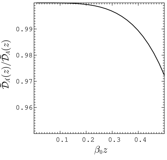
FIG. 5.: Modification of the Borel integrand to account for renormalons. We plot $\tilde{\cal D}_{A^{\prime}}(z)/\tilde{\cal D}_{A}(z)$, Eqs. (84) and (85), versus $\beta_{0}z$. We set $s=M_{Z}^{2}$ and choose the scheme fixing parameters $\delta t=\delta\beta_{2}=\delta t_{m}=0$.

VII Results

We have developed an approximation to ${\cal R}(s)$ that takes $\pi^{2}$ contributions into account and uses information about the leading renormalon singularities to try to improve the convergence of the perturbative expansion for $\tilde{\cal D}(z)$. In Fig. 6 we plot this approximation, ${\cal R}_{A}(s;\pi^{2},{\rm R\hbox{'}lons})$, versus the scheme parameter $\delta t$ with the other scheme parameters set to $\delta\beta_{2}=\delta t_{m}=0$. We overlay the plots of the pure perturbative function, ${\cal R}_{A}(M_{Z}^{2};{\rm Pert})$, and the approximation that simply takes $\pi^{2}$ contributions into account, ${\cal R}_{A}(M_{Z}^{2};\pi^{2})$. We note that ${\cal R}_{A}(s;\pi^{2},{\rm R\hbox{'}lons})$ varies by about 0.8% between its local maximum and its local minimum. This suggests that ${\cal R}(M_{Z}^{2})$ probably lies within this 0.8% range, so that one would ascribe a theoretical error of $\pm 0.8\%/2=\pm 0.4\%$ to the value of ${\cal R}(M_{Z}^{2})$.

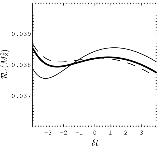
FIG. 6.: Plot of approximant ${\cal R}_{A}(s;\pi^{2},{\rm R\hbox{'}lons})$, Eq. (86), versus the scheme fixing parameter $\delta t$ with $\delta\beta_{2}=0$ and $\delta t_{m}=0$ (heavy line). We also show ${\cal R}_{A}(M_{Z}^{2};{\rm Pert})$ from Fig. 2 (light line) and ${\cal R}_{A}(M_{Z}^{2};\pi^{2})$ from Fig. 4 (dashed line).

We can take another approach to error estimation. We note that the first three coefficients of $(\beta_{0}\zeta)^{n}$ in Eq. (78) are all of order 1. That the coefficients do not appear to be growing or shrinking with $n$ is normal since the series is expected to have a radius of convergence of about 1 in the variable $\beta_{0}\zeta$. We thus expect that the uncalculated coefficient of $(\beta_{0}\zeta)^{3}$ will also be of order 1. If we add a term $1\times(\beta_{0}\zeta)^{3}$ to the series in Eq. (86), ${\cal R}_{A}(M_{Z}^{2})$ changes by an amount $\delta{\cal R}_{A}$ that can serve as an error estimate. We find ${\delta{\cal R}_{A}/{\cal R}_{A}(M_{Z}^{2};\pi^{2},{\rm R\hbox{'}lons})}\approx 0.2\%.$

We thus have three error estimates. From the $\delta t$ dependence of ${\cal R}_{A}(M_{Z}^{2};\pi^{2})$ we estimated a 0.16% error. From consideration of the likely size of the next term in $\tilde{\cal B}(\zeta)$ we estimated a 0.2% error. From the $\delta t$ dependence of ${\cal R}_{A}(M_{Z}^{2};\pi^{2},{\rm R\hbox{'}lons})$ we estimated a 0.4% error. We take the largest of these values, 0.4%, as a reasonable estimate of the theoretical error (in the spirit of a “1 $\sigma$” error).

For the central value, we take the value of ${\cal R}_{A}(s;\pi^{2},{\rm R\hbox{'}lons})$ at $\delta t=0$, which is almost exactly also the value of ${\cal R}_{A}(s;\pi^{2})$ at $\delta t=0$. This value is

$${\cal R}_{A}(M_{Z}^{2};\pi^{2},{\rm R\hbox{'}lons})_{\delta t=0}\approx(1-0.006)\times{\cal R}_{A}(M_{Z}^{2};{\rm Pert})_{\delta t=0}.$$ (87)

That is, our best estimate for $\cal R$ is renormalized down by 0.6% compared to the standard $\overline{\rm MS}$ value with a scale choice $\mu=M_{Z}$.

One often uses a measurement of ${\cal R}(M_{Z}^{2})$ to extract a value of $\overline{\alpha}_{s}(M_{Z}^{2})$. Recall that, to a good approximation, ${\cal R}(M_{Z}^{2})\propto\overline{\alpha}_{s}(M_{Z}^{2})$. Thus the value of $\overline{\alpha}_{s}(M_{Z}^{2})$ extracted from data using the “standard” $\overline{\rm MS}$ expression for $\cal R$ (with a scale choice $\mu=M_{Z}$) would be renormalized up by 0.6% if one uses the “improved” version of $\cal R$ presented here:

$$[\overline{\alpha}_{s}(M_{Z}^{2})]_{\rm improved}\approx 1.006\ [\overline{\alpha}_{s}(M_{Z}^{2})]_{\rm standard}.$$ (88)

The fractional error to be ascribed to $\overline{\alpha}_{s}(M_{Z}^{2})$ from uncertainties in the QCD perturbation theory is just the fractional error in ${\cal R}_{A}(M_{Z}^{2};\pi^{2},{\rm R\hbox{'}lons})$ estimated above as 0.4%. This is one third of the 1.3% error that we would ascribe to $\overline{\alpha}_{s}(M_{Z}^{2})$ extracted using the standard perturbative approximant ${\cal R}_{A}(M_{Z}^{2};{\rm Pert})$. The shift in Eq. (88) is about the same size as the estimated theoretical error, so it is marginally significant.

We note that the experimental error for the extraction of $\alpha_{s}$ by this method is about 5% [17], much larger than the QCD theoretical error that we estimate above. There are also sources of theoretical error not associated with QCD. According to the estimates of Hebbeker, Martinez, Passarino and Quast [18], the most important of these are a $\pm 2\%$ uncertainly from electroweak corrections and a $\pm 2\%$ uncertainly from not knowing the Higgs boson mass.

Present status of perturbative QCD evaluation of Z decay rates

The decay rate of the $Z$ boson into quark antiquark pair can be written in the following form:

$$\Gamma_{Z\rightarrow\mbox{hadrons}}=\frac{G_{F}M_{Z}^{3}}{8\sqrt{2}\pi}$$ (92)

$$\times\Biggl{\{}\sum_{f}\biggl{(}\rho_{f}v_{f}^{2}\biggl{[}(1+2X_{f})\sqrt{1-4X_{f}}+\delta_{\mbox{QCD}}^{\mbox{V}}(\alpha_{s},X_{f},X_{t})+\delta_{\mbox{QED}}^{\mbox{V}}(\alpha,\alpha_{s},X_{f})\biggr{]}$$

$$\hskip 42.67912pt+\rho_{f}a_{f}^{2}\biggl{[}(1-4X_{f})^{3/2}+\delta_{\mbox{QCD}}^{\mbox{A}}(\alpha_{s},X_{f},X_{t})+\delta_{\mbox{QED}}^{\mbox{A}}(\alpha,\alpha_{s},X_{f})\biggr{]}\biggr{)}$$

$$\quad+\ {\cal L}^{\mbox{V}}+{\cal L}^{\mbox{A}}\Biggr{\}}.$$

Here there is a sum over light quark flavors $f=u,d,s,c,b$. We define $X_{f}=m_{f}(M_{Z})^{2}/M_{Z}^{2}$ and $X_{t}=m_{t}(M_{Z})^{2}/M_{Z}^{2}$. (We use the $\overline{\rm MS}$ definition of masses.)

The vector and axial couplings of quark $f$ to the $Z$ boson are $v_{f}=\{2I_{f}^{(3)}-4e_{f}\sin^{2}\theta_{\mbox{W}}k_{f}\}$ and $a_{f}=\,2I_{f}^{(3)}$. The electroweak self-energy and vertex corrections are absorbed in the factors $\rho_{f}$ and $k_{f}$. The current status of the electroweak contributions has been discussed in detail in Ref. [3]. The small QED corrections in vector and axial channels have the form

$$\delta_{\mbox{QED}}^{\mbox{V}}=\frac{3}{4}\,e_{f}^{2}\,\frac{\alpha}{\pi}\,[1+12X_{f}+O(X_{f}^{2})]+O(\alpha^{2})+O(\alpha\alpha_{s}),$$ (93)

$$\delta_{\mbox{QED}}^{\mbox{A}}=\frac{3}{4}\,e_{f}^{2}\,\frac{\alpha}{\pi}\,[1-6X_{f}-12X_{f}\log X_{f}+O(X_{f}^{2})]+O(\alpha^{2})+O(\alpha\alpha_{s}).$$ (94)

The corrections of order $\alpha^{2}$ and $\alpha\alpha_{s}$ are discussed in Ref. [19].

It is convenient to decompose the QCD contributions into singlet and non-singlet parts and further into vector ($V$) and axial vector ($A$) contributions. The nonsinglet parts are represented by the terms $\delta_{\mbox{QCD}}^{\mbox{V}}$ and $\delta_{\mbox{QCD}}^{\mbox{A}}$, and correspond to cut Feynman graphs in which a single quark loop of flavor $f$ connects the two electroweak current operators. The singlet contributions correspond to graphs with the electroweak currents in separate quark loops mediated by gluonic states. In the singlet contributions one does not have a single sum over a flavor $f$. These contributions are represented by the terms ${\cal L}^{\mbox{V}}$ and ${\cal L}^{\mbox{A}}$.

The nonsinglet QCD contribution in the vector channel to order $\alpha_{s}^{3}$ can be written in the form

$$\delta_{\mbox{QCD}}^{\mbox{V,ns}} = \frac{\alpha_{s}}{\pi}\,\left[1+12\,{X}_{f}\right]$$ (97)

$$+\biggl{(}\frac{\alpha_{s}}{\pi}\biggr{)}^{2}\left[1.40923+104.833\,{X}_{f}+\sum_{v}F^{(2)}(X_{v})+G^{(2)}(X_{t})\right]$$

$$+\biggl{(}\frac{\alpha_{s}}{\pi}\biggr{)}^{3}\left[-12.76706+547.879\,{X}_{f}+\sum_{v}F^{(3)}(X_{v})+G^{(3)}(X_{t})\right].$$

In this formula, $\alpha_{s}$ denotes the running $\overline{\rm MS}$ coupling in five flavor theory evaluated at $M_{Z}$. The transformation relation for different number of flavors and different scales, as well as the relation between the $\overline{\rm MS}$ running mass and the pole mass can be found in Ref. [20].

The order $\alpha_{s}^{2}$ and $\alpha_{s}^{3}$ terms have been evaluated in the limit of vanishing light quark masses and infinitely large top mass in Refs. [10, 11]. These contributions, $(\alpha_{s}/\pi)+1.40923\,(\alpha_{s}/\pi)^{2}-12.76706\,(\alpha_{s}/\pi)^{3}$, are the {vector,nonsinglet} part of the perturbative series analyzed in the main body of this paper.

The terms proportional to ${X}_{f}$ represent the leading corrections to the approximation $X_{f}=0$, as given in Ref. [4].

The function $F^{(2)}(X_{v})$ arises from three-loop diagrams containing an internal quark loop with a quark of flavor $v=u,d,s,c,b$ propagating in it (while the quark of flavor $f$ couples to the weak currents). This function represents the corrections to the approximation $X_{v}=0$. These contributions are already small, so it suffices to approximate $X_{f}$ by 0 in $F^{(2)}(X_{v})$. In fact, numerically [5],

$$F^{(2)}(X_{v})\approx{X}_{v}^{2}\times\left\{-0.474894-\log{X}_{v}+\sqrt{{X}_{v}}\left[-0.5324+0.0185\log{X}_{v}\right]\right\}$$ (98)

is so small that the whole function could be neglected.

The function $G^{(2)}(X_{t})$ represents the contribution of virtual top quark loops inside three-loop cut Feynman diagrams. These contributions are small since the top quark is nearly decoupled from the theory. Thus it suffices to approximate $X_{f}$ by 0 in $G^{(2)}(X_{t})$. Numerically, one finds [5]

$$G^{(2)}(X_{t})\approx{{X}_{t}^{-1}}\times\left\{{44\over 675}+{2\over 135}\log{X}_{t}-\sqrt{{X}_{t}^{-1}}\left[0.001226+0.001129\log{X}_{t}\right]\right\}.$$ (99)

The first two terms in the right hand side of eq.(99) have also been obtained using the large mass expansion method [21].

At order $\alpha_{s}^{3}$, there can be two internal quark loops. However, it suffices to consider only one loop with a nonzero light quark mass at a time, or one top quark loop with all light quark masses set to zero. Then we can define functions $F^{(3)}(X_{v})$ and $G^{(3)}(X_{t})$ analogously to $F^{(2)}(X_{v})$ and $G^{(2)}(X_{t})$. For $F^{(3)}(X_{v})$ the following small mass expansion is obtained in Ref. [4]:

$$F^{(3)}(X_{v})\approx-6.12623{X}_{f}.$$ (100)

For $G^{(3)}(X_{t})$ the following large mass expansion has been obtained in Ref [22]:

$$G^{(3)}(X_{t})\approx{{X}_{t}^{-1}}\times[-0.1737-0.2124\log{X}_{t}-0.0372\log^{2}{X}_{t}].$$ (101)

The nonsinglet contribution in the axial channel is the same as the one in the vector channel except that the contributions proportional to $X_{f}$ [4, 5] are different:

$$\delta_{\mbox{QCD}}^{\mbox{A,ns}} = \frac{\alpha_{s}}{\pi}\,\left[1-22\,{X}_{f}\right]$$ (104)

$$+\biggl{(}\frac{\alpha_{s}}{\pi}\biggr{)}^{2}\left[1.40923-85.7136\,{X}_{f}+\sum_{v}F^{(2)}(X_{v})+G^{(2)}(X_{t})\right]$$

$$+\biggl{(}\frac{\alpha_{s}}{\pi}\biggr{)}^{3}\left[-12.76706+(\mbox{unknown})\,{X}_{f}+\sum_{v}F^{(3)}(X_{v})+G^{(3)}(X_{t})\right].$$

We now turn to the singlet contributions, which start at order $\alpha_{s}^{2}$:

$${\cal L}^{\mbox{V/A}}={\cal L}_{2}^{\mbox{V/A}}\left(\alpha_{s}\over\pi\right)^{2}+{\cal L}_{3}^{\mbox{V/A}}\left(\alpha_{s}\over\pi\right)^{3}+\cdots.$$ (105)

At order $\alpha_{s}^{2}$, there is no vector contribution,

$${\cal L}_{2}^{\mbox{V}}=0,$$ (106)

while the axial contributions from $u$ and $d$ quarks and from $c$ and $s$ quarks vanish in the limit of vanishing quark masses. This is because in the Standard Model the quarks in a weak doublet couple with the opposite sign to the weak axial current. However, the contribution from the $t$,$b$ doublet is significant because of the large mass splitting [23]:

$${\cal L}_{2}^{\mbox{A}} = -\frac{37}{12}-\log X_{t}+\frac{7}{81}X_{t}^{-1}+0.013X_{t}^{-2}$$ (108)

$$+{X}_{b}\,(18+6\,\log X_{t})-\frac{{X}_{b}}{X_{t}}\,\biggl{(}\frac{80}{81}+\frac{5}{27}\log X_{t}\biggr{)}.$$

Here the corrections proportional to ${X}_{b}$ have been calculated in Ref. [24].

At order $\alpha_{s}^{3}$, both channels contribute. The vector contribution in the limit of massless light quarks is [11]

$${\cal L}_{3}^{\mbox{V}}=-0.41318\,\biggl{(}\sum_{f}v_{f}\biggr{)}^{2}+\left(0.02703\,{X}_{t}^{-1}+0.00364\,{X}_{t}^{-2}+O(X_{t}^{-3})\right)\,v_{t}\sum_{f}v_{f}.$$ (109)

The sums here run over light quark flavors $f=u,d,s,c,b$. The terms proportional ${X}_{t}^{-1},{X}_{t}^{-2}$ were computed in Ref. [22] and turn out to be negligible.

In the axial channel, the order $\alpha_{s}^{3}$ singlet contribution in the large top mass expansion reads [25, 22, 3]

$${\cal L}_{3}^{\mbox{A}}=-15.98773-\frac{67}{18}\log X_{t}+\frac{23}{12}\log^{2}X_{t}.$$ (110)

Corrections for a nonzero $b$ quark mass are not yet known. However, at the level of precision of this paper, they are not expected to be significant.

REFERENCES

[1] D. E. Soper in
QCD and High Energy Interactions,
Proceedings of the XXX Rencontre de Moriond, Les Arcs, 1995,
edited by J. Tran Thanh Van
(Editions Frontières, Gif-sur-Yvette Cedex, France, 1995,
to be published)
[2] CDF Collaboration,F. Abe et al.,
Phys. Rev. Lett. 74, 2626 (1995);
D0 Collaboration, F. Abe et al.,
Phys. Rev. Lett. 74, 2632 (1995);
[3] B. A. Kniehl,
Int. J. Mod. Phys. A10 (1995) 443.
[4] K. G. Chetyrkin and J. H. Kühn,
Phys. Lett. B248 (1990) 359;
K. G. Chetyrkin, J. H. Kühn and A. Kwiatkowski,
Phys. Lett. B282 (1992) 221;
L. R. Surguladze,
University of Oregon preprint OITS-554, 1994,
e-Print Archive: hep-ph /9410409.
[5] D. E. Soper and L. R. Surguladze,
Phys. Rev. Lett. 73, (1994) 2958;
B. A. Kniehl, Phys. Lett. B237 (1990) 127;
A. H. Hoang, M. Jezabek, J. H. Kühn, T. Teubner,
Phys. Lett. B 338, 330 (1994).
[6] G. t’Hooft, Nucl. Phys. B 61 (1973) 455;
W. Bardeen, et al., Phys. Rev. (1978) 18, 3998.
[7] P. M. Stevenson, Phys. Lett. B100 (1981) 61;
Phys. Rev. D23 (1981) 2916.
[8] L. R. Surguladze and M. A. Samuel, Rev. Mod. Phys. (to be published), e-print archive
hep-ph/9508351.
[9] O. V. Tarasov, A. A. Vladimirov, and A. Yu. Zharkov,
Phys. Lett. B 93 (1980) 429.
[10] K. G. Chetyrkin, A. L. Kataev and F. V. Tkachov,
Phys. Lett. B85 (1979) 277;
M. Dine and J. Sapirstein, Phys. Rev. Lett.,
43 (1979) 668;
W. Celmaster and R. Gonsalves, Phys. Rev. Lett.
44 (1980) 560.
[11] L. R. Surguladze and M. A. Samuel,
Phys. Rev. Lett. 66 (1991) 560;
S. G. Gorishny, A. L. Kataev and S. A. Larin,
Phys. Lett. B259 (1991) 144.
See also L. R. Surguladze and M. A. Samuel,
Phys. Lett. B309 (1993) 157;
[12]
G. Altarelli, P. Nason and G. Ridolfi, preprint CERN-TH-7537-94, 1994,
(e-Print Archive: hep-ph/9501240)
[13] A. H. Mueller, Nucl. Phys. B250 (1985) 327.
[14] F. Le Diberder and A. Pich,
Phys. Lett. B 286, 147 (1992).
[15] A. H. Mueller, in Proc. QCD 20 Years Later
(Aachen, Germany, 1992),
Ed. P. M. Zerwas and H. A. Kastrup, Vol.1, p.162.
[16] A. I. Vainshtein and V. I. Zakharov,
Phys. Rev. Lett. 73 (1994) 1207.
[17] J. Casaus in
QCD and High Energy Interactions,
Proceedings of the XXX Rencontre de Moriond, Les Arcs, 1995,
edited by J. Tran Thanh Van,
(Editions Frontières, Gif-sur-Yvette Cedex, France, 1995, to be
published).
[18] T. Hebbeker, M. Martinez, G. Passarino and G. Quast, Phys. Lett. B331, 165 (1994).
[19] A. L. Kataev, Phys. Let. B287 (1992) 209.
[20] L. R. Surguladze, Phys. Lett. B341 (1994) 60.
[21] K. G. Chetyrkin, Phys. Lett. B307 (1993) 169.
[22] S. A. Larin, T. van Ritbergen and J. A. M. Vermaseren,
Nucl. Phys., B438 (1995) 278.
[23] B. A. Kniehl and J. H. Kühn,
Phys. Lett. B224 (1989) 229;
Nucl. Phys. B329 (1990) 547.
[24] K. G. Chetyrkin and A. Kwiatkowski,
Phys. Lett. B305 (1993) 285.
[25] K. G. Chetyrkin and O. V. Tarasov,
Phys. Lett. B327 (1994) 114.