UdeM-TH-95

McGill/95-49

Brown-HET-1023

hep-ph/9511252

November 1995

PARTICLE PRODUCTION

IN A HADRON COLLIDER RAPIDITY GAP:

THE HIGGS CASE

JEAN-RENÉ CUDELL

Dept. of Physics, McGill University, Montréal QC, Canada H3A 2T8

and Dept. of Physics, Brown University , Providence RI 02906, U.S.A.

cudell@hep.physics.mcgill.ca

and

OSCAR F. HERNÁNDEZ

Labo. de Physique Nucléaire, Université de Montréal, Montréal QC Canada H3C 3J7

oscarh@lps.umontreal.ca

ABSTRACT

Production of rare particles within rapidity gaps has been proposed as a background-free signal for the detection of new physics at hadron colliders. No complete formalism accounts for such processes yet. We study a simple lowest-order QCD model for their description. Concentrating on Higgs production, we show that the calculation of the cross section $pp\rightarrow ppH$ can be embedded into existing models which successfully account for diffractive data. We extend those models to take into account single and double diffractive cross sections $pp\rightarrow HX_{1}X_{2}$ with a gap between the fragments $X_{1}$ and $X_{2}$. Using conservative scenarios, we evaluate the uncertainties in our calculation, and study the dependence of the cross section on the gap width. We predict that Higgs production within a gap of 4 units of rapidity is about 0.3 pb for a 100 GeV Higgs at the Tevatron, and almost 2 pb for a 400 GeV Higgs within a gap of 6 units at the LHC with $\sqrt{s}$=14 TeV.

1. Rapidity gaps as a detection tool

At hadron colliders, rare high-$Q^{2}$ processes can be produced in the usual hard collision picture, where two partons, one from each nucleon, collide head-on and annihilate into the rare particle one is trying to produce. The big drawback of such a production mechanism is that hadrons cannot simply loose their partons, since the annihilation of two partons leaves the initial nucleons in a coloured state. This means that they will not fragment independently, but rather that a colour string will link them. When they pull apart, the spectator partons will break the string. Hadronic matter will then populate most of the central phase space. However in roughly 10% of the hard scattering events at HERA, further interactions neutralize the colour of the proton fragments, and lead to large rapidity gaps [1].

If one manages to produce a rare particle without changing the colour of the nucleons, then very little hadronic activity should be present in the event. Of course, both nucleons will still fragment, as the production of a heavy particle imbalances the kinematics of their partons, but the two fragmentations will be independent, as they are not correlated by colour strings. Hence the produced hadrons will follow the direction of the initial nucleons and there will be a large rapidity gap with no hadronic remnants. The rare particle will often be produced within the gap, and hence its decay should be essentially background-free. Bjorken [2] has suggested using such rapidity gaps as a means of detecting new physics.

Colour-singlet exchange between protons is in fact a very common event, and it has been known and observed for a long time. Indeed, the simplest kind of event with a rapidity gap is the elastic scattering $pp\rightarrow pp$, which accounts for about 20% of the total cross section at the Tevatron [3, 4]. Another 20% of the cross section is due to single diffractive scattering $pp\rightarrow pX$, and to double diffractive scattering $pp\rightarrow X_{1}X_{2}$, both processes leading to a large rapidity gap between produced hadrons. Hence the study of rare particle production in a rapidity gap can be seen as the inclusion of a high-mass component into soft, low-$Q^{2}$ diffractive physics.

Several attempts have been made to describe this process within a structure function formalism, following Ingelman and Schlein [5], and the demonstration by UA8 that hard diffractive scattering does exist [6]. These works use a pomeron structure function, and treat the pomeron in a way similar to a photon. The major drawback of this approach is that we do not know what the pomeron is made of, and whether the concept of structure function holds for it. Similarly, the pomeron structure function is not well measured, even if it exists, and its flux factor is also subject to question [7].

The cleanest estimate of Higgs production is presumably that due to Bialas and Landshoff [10], where they perform a two-gluon exchange calculation. However, their calculation suffers from a few drawbacks:
$\bullet$ They rely on the Landshoff-Nachtmann [17] model of the gluon propagator, which is taken to be a falling exponential. Although this model has reasonable phenomenological support, it is not adapted to higher-order calculations;
$\bullet$ In the case of diffractive scattering, i.e. when the proton breaks up, they rely heavily on Regge theory, as their cross section converges only because of the non-zero Regge slope;
$\bullet$ They totally neglect exchanges involving several quarks in each proton ;
$\bullet$ They neglect the effects of the longitudinal parton kinematics, which is essential for heavy particle production.

In this paper we remedy all the above problems: we introduce new form factors, which describe diffractive scattering, and explain how the longitudinal kinematics comes into play. We keep the exact kinematics of the problem, and show that the cross section are IR finite even in perturbative QCD. We then estimate the size of the cross section, and obtain a result surprisingly close to that of Bialas and Landshoff.

It is well known that lowest-order QCD produces surprisingly good estimates of diffractive processes. In the present case, we tune the form factors so that they reproduce the measured elastic and diffractive cross sections. We then embed Higgs production within soft cross sections.

Our first task will then be (in Section 2) to review the calculation of the elastic cross sections [8, 9], and to extend it to single- and double- diffractive processes. We will then (in Section 3) lay out the formalism which embeds high-mass particle production in diffractive physics. Although the method is quite general and can be used for a variety of processes, we shall concentrate in Section 4 on Higgs production. We show that our treatment leads to a cross section which is about 20% higher than the estimate of Bialas and Landshoff, and that the details of the infrared region do not play an overwhelming role in the determination of the total rate. We also find that the evaluation of the elastic cross section depends very little on the details of the model. We then evaluate the inelastic diffractive contribution $pp\rightarrow X_{1}X_{2}H$, which turns out to be a factor $\sim 3$ larger than the elastic one. The final section contains a summary of our results and conclusions.

2. QCD models of diffractive physics

Colour-singlet interactions between nucleons is an old topic. Regge theory attributes these interactions to the exchange of mesons, grouped into Regge trajectories according to their quantum numbers. In the high-$s$ limit, one expects the hadronic amplitude to be a sum of simple poles, each pole corresponding to the exchange of the particles lying on a given Regge trajectory:

$${\cal A}(s,t)=\sum_{i}\beta_{i}^{2}(t)\ s^{\alpha_{i}(t)}\xi(\alpha_{i}(t))$$ (2.1)

with $\xi$ the Regge signature factor. ${\cal A}(s,t)$ is normalised so that the elastic cross section is given by $d\sigma_{el}/dt=|{\cal A}|^{2}/16\pi^{2}$, which through the use of the optical theorem gives a total cross section $\sigma_{tot}=Im\left({\cal A}(s,t=0)\right)$.

The leading meson trajectories are the (degenerate) trajectories of the $\rho$ and $f$ mesons, clearly present when plotting the meson states in a $J$ vs $M^{2}$ plane. When continued to negative values of $M^{2}$, these trajectories are responsible for the fall-off of the total cross section at small $s$, $\sigma_{tot}\sim 1/\sqrt{s}$. At higher energies, the cross sections grow, and the most natural assumption is that another term in Eq. (2.1) is responsible for that rise although there is no observed trajectory to guide us. Hence one new Regge trajectory was invented, the pomeron, which is whatever makes the total cross section rise at high energy (at 1800 GeV, more than 99% of the total cross section is due to pomeron exchange). In modern day QCD, non-mesonic exchanges are attributed to multi-gluon exchanges, which naturally produce a rising elastic cross section in perturbation theory.

Several other properties of high-$s$ colour-singlet exchanges can be inferred from data [11]:
$\bullet$ The pomeron trajectory of Eq. (2.1) is well fitted from $\sqrt{s}=5$ GeV to $1800$ GeV, and from $t=0$ to $-1$ GeV² to the form

$$\alpha_{P}(t)=1.08+0.25t$$ (2.2)

$\bullet$ The pomeron coupling to protons, $\beta_{P}(t)$, is well approximated by the coupling of photons, i.e. by the Dirac elastic form factor:

$$F_{1}(t)={(3.53-2.79t)\over(3.53-t)\ (1-t/0.71)^{2}}$$ (2.3)

$\bullet$ Colour-singlet exchanges are factorizable: the ratio of the differential cross section for $pA\rightarrow XA$ to that for $pA\rightarrow pA$ does not depend on $A$ [12]. Another related property is the quark counting rule: hadronic cross sections are proportional to the number of valence quarks contained in the hadron. This is tested not only in $\pi p$ vs $pp$ cross sections, but also in cross sections involving strange quarks, e.g. $2\sigma_{tot}(\Omega^{-}p)-\sigma_{tot}(\Sigma^{-}p)$ can be predicted from $\sigma_{tot}(pp)$, $\sigma_{tot}(\pi p)$ and $\sigma_{tot}(Kp)$ [13].

2.1. QCD models for elastic and total cross sections

The simplest QCD colour-singlet exchange consists of two gluons [14]. and is shown in Fig. 1.

Figure 1: The lowest order Feynman diagrams for $pp$ colour-singlet exchange

If we exchange these gluons between quarks, we obtain the following (IR divergent) amplitude [9]:

$${\cal A}_{q}(\hat{s},\hat{t})={8i\over 9}\ \alpha_{S}^{2}s\int d^{2}{\bf k}_{a}d^{2}{\bf k}_{b}{d{\cal A}_{q}\over d^{2}{\bf k}_{a}d^{2}{\bf k}_{b}}$$ (2.4)

with

$${d{\cal A}_{q}\over d^{2}{\bf k}_{a}d^{2}{\bf k}_{b}}=\delta^{(2)}({\bf\Delta}-{\bf k}_{a}-{\bf k}_{b}){1\over({{\bf k}_{a}}^{2}-\sigma_{a})}\times{1\over({{\bf k}_{b}}^{2}-\sigma_{b})}$$ (2.5)

Here bold face variables represent transverse momenta. The transverse momenta ${\bf k}_{a}$ and ${\bf k}_{b}$ are the components of the gluon momenta transverse to the direction of the quarks and ${\bf\Delta}$ is the total momentum exchanged by the quarks (${\bf\Delta}^{2}=t$). We have introduced two gluon squared masses $\sigma_{a}$ and $\sigma_{b}$.

The quark counting rule suggests that we describe a proton as made of its 3 valence quarks, and that the sea quarks do not contribute much to these processes (or that they are generated by higher orders). One can then show that quark-quark scattering can be simply embedded into the proton [9, 8]. The elastic amplitude for two-gluon exchange between two protons has been shown to be:

$${\cal A}_{2}={8i}\alpha_{S}^{2}\hat{s}\int d^{2}{\bf k}_{a}d^{2}{\bf k}_{b}{d^{2}{\cal A}^{q}_{2}\over d^{2}{\bf k}_{a}d^{2}{\bf k}_{b}}[{\cal E}_{1}({\bf k}_{a}+{\bf k}_{b})-{\cal E}_{2}({\bf k}_{a},{\bf k}_{b})]^{2}$$ (2.6)

${\cal E}_{1}$ and ${\cal E}_{2}$ are two of the three form factors that can occur in the valence quark description of a proton. Each of these form factors correspond to the situation where 1, 2 or 3 quarks get hit by gluons. One can write their expression in terms of the proton wavefunction $\psi$:

$${\cal E}_{1}({\bf k}) = \int d{\cal M}|\psi(\beta_{j},{\bf r}_{j})|^{2}e^{i{\bf k}.{\bf r}_{k}}$$

$${\cal E}_{2}({\bf k}_{a},{\bf k}_{b}) = \int d{\cal M}|\psi(\beta_{j},{\bf r}_{j})|^{2}e^{i{\bf k}_{a}.{\bf r}_{k}+i{\bf k}_{b}.{\bf r}_{l}}$$

$${\cal E}_{3}({\bf k}_{a},{\bf k}_{b},{\bf k}_{c}) = \int d{\cal M}\ |\psi(\beta_{j},{\bf r}_{j})|^{2}e^{i{\bf k}_{a}.{\bf r}_{k}+i{\bf k}_{b}.{\bf r}_{l}+i{\bf k}_{c}.{\bf r}_{m}}$$ (2.7)

where $\beta_{j}$ is the fraction of longitudinal momentum (similar to Bjorken $x$), and ${\bf r}_{j}$ is the transverse position of quark $j$. The natural integration measure $d{\cal M}$ is defined as:

$$d{\cal M}=[\prod_{j=1,n_{q}}d\beta_{j}d^{2}{\bf r}_{j}]\delta^{(2)}(\sum_{j}\beta_{j}{\bf r}_{j})\delta(\sum_{j}\beta_{j}-1)$$ (2.8)

The first delta function defines the center of momentum of the hadron, whereas the second one enforces longitudinal-momentum conservation. Assuming that hadrons are made of valence quarks only, we normalise the wavefunction according to:

$${\cal E}_{1}(0)=\int d{\cal M}|\psi(\beta_{j},{\bf r}_{j})|^{2}=1$$ (2.9)

These expressions become useful once one realises that the form factor ${\cal E}_{1}$ also occurs in the elastic $\gamma^{*}p$ cross section and is none other than the Dirac elastic form factor in Eq. (2.3). Hence one of the form factors is determined. Furthermore, ${\cal E}_{2}$ and ${\cal E}_{3}$ are related to ${\cal E}_{1}$ by the following properties:

$${\cal E}_{2}({\bf k}_{a},0) = {\cal E}_{1}({\bf k}_{a})$$

$${\cal E}_{3}({\bf k}_{a},{\bf k}_{b},0) = {\cal E}_{2}({\bf k}_{a},{\bf k}_{b})$$ (2.10)

These properties ensure the IR finiteness of Eq. (2.6). One can either calculate these form factors using a model for the proton wave function [9], or use a simple parametrisation, which takes into account both the infrared and the symmetry properties of the form factors: one simply needs to make an ansatz for ${\cal E}_{3}$ and obtain ${\cal E}_{2}$ from Eq. (2.10). We take

$${\cal E}_{3}({\bf k}_{a},{\bf k}_{b},{\bf k}_{c})={\cal E}_{1}\left({\bf k}_{a}^{2}+{\bf k}_{b}^{2}+{\bf k}_{c}^{2}-c({\bf k}_{a}\cdot{\bf k}_{b}+{\bf k}_{a}\cdot{\bf k}_{c}+{\bf k}_{b}\cdot{\bf k}_{c})\right)$$ (2.11)

where $c$ is an arbritrary number which can be shown to be of order one in the proton case [9].

We have written the form factors as functions of the gluon momenta to manifestly show that Eqs. (10) hold as the gluon momenta go on shell. However the form factor comes from the proton wavefunction and can only depend on quark variables. Hence ${\bf k}_{a},~{}{\bf k}_{b},~{}{\bf k}_{c}$ should be thought of as differences between initial- and final-quark transverse momenta.

At this stage, one is in a situation to describe elastic scattering and hence, through the use of the optical theorem, total cross sections. The model contains two free parameters, $\alpha_{S}$ and $c$, which we can tune to reproduce the data. One can then look at the shape of the differential elastic cross section to check whether the model makes sense. Unfortunately, it is well-known [8, 9, 15] that the shape of the cross section comes out wrong: its logarithmic slope at the origin is infinite, and its curvature is too big.

One may be tempted to look into higher order corrections for a solution to this problem. Indeed, $\alpha_{S}$ is not small, and the perturbative series contains terms of order $\alpha_{S}^{n+1}\log^{n}s$ which clearly can become big at large $s$. These terms can be resummed using the BFKL techniques [16], but such formalism cannot account for diffractive scattering at low momentum transfers, where unfortunately most of the cross section is concentrated. The most obvious problem is that the rise of the cross section predicted by leading-log-$s$ perturbative QCD is entirely different from that which is observed in data, as its leading contribution to the hadronic amplitude goes like $s^{1+2.65\alpha_{s}}$. Secondly, the slope of the pomeron trajectory $\alpha^{\prime}=0.25$ GeV^-2 introduces a scale of the order of $1/\sqrt{\alpha^{\prime}}\approx 2$ GeV, which comes in the description of the $t$-dependence of the hadronic amplitude. No such scale is present in perturbative QCD, hence the differential elastic cross section retains its wrong shape. Finally, the amplitude is not factorizable: this is in fact a consequence of the infrared finiteness of the answer. Quark-quark scattering via gluon exchange diverges for massless gluons. Nevertheless, hadron-hadron scattering is infrared finite, as the colour of the hadron gets averaged for very long wavelength gluons. Hence there is a contribution that comes from the diagrams where gluons are exchanged between different quarks in the hadron. These diagrams feel the hadronic wavefunction, and hence their contribution depends on the target.

Even the lowest-order two-gluon exchange cross section fails to reproduce the factorizability of the hadronic amplitude. This prompted Landshoff and Nachtmann [17] to postulate that gluons have an intrinsic propagation length $1/\mu_{0}$ smaller than typical hadronic sizes. The propagator hence becomes:

$$D(k^{2})=d(k^{2}/\mu_{0}^{2})/\mu_{0}^{2}$$ (2.12)

with $\lim_{x\rightarrow 0}xd(x)=0$. In that case, the diagrams in which the gluons couple to different quarks are suppressed by a factor $\sim(25\ GeV^{-2})\mu_{0}^{2}$ with respect to those in which the gluons couple to the same quark line, and factorisation can be restored, for $\mu_{0}\sim 1$ GeV.

This kind of picture has recently been questioned on theoretical grounds [18], but it seems to remain the only one available which reproduces the observed properties of the pomeron. In the following, rather than worrying about the ultimate nature of the pomeron, we shall adopt the following pragmatic approach: we are after rates for the production of rare particles produced in a rapidity gap. This is very similar to single-diffractive processes and elastic processes, except that we need to insert a rare particle production vertex in the diagram. The best phenomenological description of such processes is two-gluon exchange, multiplied by a pomeron s-dependence given by Eq. (2.1). We shall first set up the lowest-order perturbative calculation of Higgs production via two-gluon exchange. We shall then evaluate the importance of the IR region by using a constituent-gluon propagator which matches to the perturbative one at high $k^{2}$ [19]. The model hence contains several parameters: $\alpha_{S}$, $c$ and a non perturbative scale $\mu_{0}$. We shall tune these parameters to the highest-energy data available, reproducing the total, elastic and diffractive cross sections at the Tevatron. Hence our calculation of Higgs production at the LHC will be parameter-free.

Note that this procedure also factors in the gap survival. Indeed, diffractive cross sections surely produce a gap, and the final-state multiple interactions which may spoil it are taken into account by our tuning of the parameters. As the kinematics of the process we are considering is rather similar to diffractive scattering, we expect that the choice of parameters which accounts for gaps in diffractive scattering will also lead to gaps in Higgs production.

2.2. A QCD model for inelastic diffractive cross sections

Before embarking into the afore-mentioned fit, we need to develop the formalism needed to describe inelastic diffractive cross sections, i.e. those in which a proton gets hit by a colour singlet, but nevertheless fragments. The main ingredient needed is a new form factor for the proton.

Hence we want to describe the process $p\rightarrow X$ instead of $p\rightarrow p$. The simplest way to do this is to square the amplitude, and to recognise that the cross section, including all the interference terms in the final state, is similar to the elastic amplitude resulting from 4-gluon exchange, with gluons arranged in two singlets.

To calculate the corresponding form factor, one has to notice that one-photon exchange leads to an ${\cal E}_{1}$ form factor. The two-gluon form factor can then be built by squaring the one-photon exchange diagram, and removing the intermediate proton. This can lead to an ${\cal E}_{1}$ form factor, if the same quark is hit in the two interfering diagrams, or to an ${\cal E}_{2}$ form factor, if different quarks are hit. Similarly, an ${\cal E}_{2}$ convoluted with an ${\cal E}_{1}$ will give either an ${\cal E}_{2}$, or an ${\cal E}_{3}$. In the case of the calculation of the elastic form factor, there is an extra complication coming from the colour algebra. However, in the case at hand, the colour algebra is trivial, because we are exchanging colour-singlets, and hence the colour factor is factorised between the two sides of the diagram. Therefore, after we recognise that the elastic form factors are given by 9 terms, three ${\cal E}_{1}$ and six ${\cal E}_{2}/2$, we can simply write down the 81 possible interferences, and decide by inspection which form factor will describe them.

More formally, one first needs to assume that in diffractive scattering one goes through an intermediate state, call it $Y$, described by a wave-function $\psi_{Y}$. The only change in the preceeding formulae (2.7) then occurs in the substitution $|\psi(\beta_{j},r_{j})|^{2}\rightarrow\psi^{*}_{p}(\beta_{j},r_{j})\psi_{Y}(\beta_{j},r_{j})$. This means that we are not going to describe intermediate states which have a mass very different from that of the proton, as their production necessitates a change in the longitudinal momentum. Hence the cross section we are calculating represents the bulk of diffractive scattering, but does not reproduce the high-mass tail. This tail presumably comes from higher-order diagrams, be they 3-pomeron vertices or gluon radiation[20, 12].

Now, in elastic scattering, the form factor describing $p\rightarrow p$ is $3({\cal E}_{1}(t)-{\cal E}_{2}(t))$. This comes from $9\times 2$ diagrams similar to those of Fig. 1, as each gluon can be attached to 3 different quarks. The form factor describing $p\rightarrow Y$ is the similar, with e.g. ${\cal E}_{1}$ given by

$${\cal E}_{1}({\bf k})=\int d{\cal M}\psi^{*}_{p}(\beta_{j},r_{j})\psi_{Y}(\beta_{j},r_{j})e^{i{\bf k}.{\bf r}_{k}}$$ (2.13)

Squaring the amplitude, we obtain the square of these form factors. Let us for instance concentrate on the ${\cal E}_{1}\times{\cal E}_{2}$ term shown in Fig. 2.

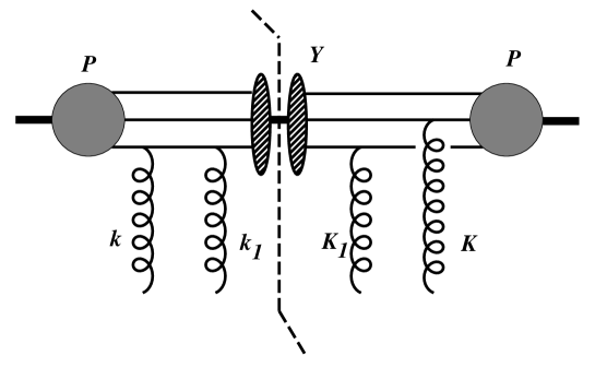
Figure 2: One of the 81 interference terms contributing to the inelastic diffractive form factor

It corresponds to the expression:

$$\sum_{Y}{\cal E}_{1}({\bf k}+{\bf k}_{1}){\cal E}_{2}({\bf K}_{1},{\bf K}) = \sum_{Y}\int[\prod_{j=1,n_{q}}d\beta_{j}d{\bf r}_{j}]\delta^{(2)}(\sum_{j}\beta_{j}{\bf r}_{j})\delta(\sum_{j}\beta_{j}-1)$$ (2.14)

$$\psi^{*}_{p}(\beta_{j},{\bf r}_{j})\psi_{Y}(\beta_{j},{\bf r}_{j})e^{i({\bf k}+{\bf k}_{1}).{\bf r}_{1}}$$

$$\times [\prod_{l=1,n_{q}}dB_{l}d{\bf R}_{l}]\delta^{(2)}(\sum_{l}B_{l}{\bf R}_{l})\delta(\sum_{l}B_{l}-1)$$

$$\psi_{Y}^{*}(B_{l},{\bf R}_{l})\psi_{p}(B_{l},{\bf R}_{l})e^{i{\bf K}_{1}.{\bf R}_{1}+{\bf K}.{\bf R}_{2}}$$

The completeness relation for the wavefunctions reads:

$$f(\beta_{l},{\bf r}_{l})=\sum_{Y}\int[\prod_{j=1,n_{q}}dB_{j}d{\bf R}_{j}]\delta^{(2)}(\sum_{j}B_{j}{\bf R}_{j})\delta(\sum_{j}B_{j}-1)$$

$$\psi_{Y}(\beta_{l},{\bf r}_{l})\psi_{Y}^{*}(B_{j},{\bf R}_{j})f(B_{j},{\bf R}_{j})$$ (2.15)

Hence formula (2.14) becomes:

$$\sum_{Y}{\cal E}_{1}({\bf k}+{\bf k}_{1}){\cal E}_{2}({\bf K}_{1},{\bf K}) = \int d{\cal M}e^{i({\bf k}+{\bf k}_{1}).{\bf r}_{1}}|\psi_{p}(b_{l},{\bf r}_{l})|^{2}e^{i{\bf K}_{1}.{\bf r}_{1}+{\bf K}.{\bf r}_{2}}$$ (2.16)

$$= {\cal E}_{2}({\bf k}+{\bf k}_{1}+{\bf K}_{1},{\bf K})$$

All the other 80 interference terms can be worked out similarly, and we get the form factor in the inclusive case from the square of the amplitudes.

Noting that the four momenta entering the form factor have to sum to zero (as we are squaring an amplitude, the initial and the final states must be identical), we use the short-hand notation: ${\cal E}_{2}({\bf l})\equiv{\cal E}_{2}({\bf l},-l)$, ${\cal E}_{3}({\bf l},{\bf L})\equiv{\cal E}_{3}({\bf l},{\bf L},-{\bf l}-{\bf L})$. We then obtain the following:

$$3 {\cal F} ({\bf k},{\bf k}_{1},{\bf K}_{1},{\bf K})=3\ [1-{\cal E}_{2}({\bf k})-{\cal E}_{2}({\bf k}_{1})-{\cal E}_{2}({\bf K}_{1})-{\cal E}_{2}({\bf K})$$

$$+ 2{\cal E}_{2}({\bf k}+{\bf k}_{1})+{1\over 2}{\cal E}_{2}({\bf k}+{\bf K})+{1\over 2}{\cal E}_{2}({\bf k}+{\bf K}_{1})$$

$$- {\cal E}_{3}({\bf k},{\bf k}_{1})-{\cal E}_{3}({\bf K},{\bf K}_{1})+{1\over 2}{\cal E}_{3}({\bf k}_{1},{\bf K}_{1})+{1\over 2}{\cal E}_{3}({\bf k},{\bf K}_{1})+{1\over 2}{\cal E}_{3}({\bf k},{\bf K})+{1\over 2}{\cal E}_{3}({\bf K},{\bf k}_{1})]$$

Note that we recover the same IR behaviour of the square form factor as we had for its elastic components: ${\cal F}({\bf k}_{1},{\bf k}_{2},{\bf k}_{3},{\bf k}_{4})\rightarrow 0$ for any ${\bf k}_{i}^{2}\rightarrow 0$. This insures the infrared finiteness of the answer.

The diffractive cross section then has the same form as the square of the elastic amplitude, except that the form factor $81[{\cal E}_{1}-{\cal E}_{2}]^{4}$ gets replaced by $9{\cal F}^{2}$.

2.3. Best values of parameters

We are now in a position to fix the parameters of the model. As we need to extrapolate to the LHC, we use Tevatron data. The fits we obtain are good to about $10\%$ in the perturbative case. Slightly better results are obtained if we smooth the infrared region of the propagator, using a constituent-gluon propagator, as explained at the end of Section 2.1.

Table 1: Diffractive data

experiment	$\sigma_{tot}$ (mb)	$\sigma_{el}$ (mb)	$2\sigma_{sd}$ (mb)
CDF [3]	$80.03\pm 2.24$	$19.7\pm 0.85$	$9.46\pm 0.44$
E710 [4]	$72.2\pm 2.7$	$16.6\pm 0.7$	$9.37\pm 2.9$

The E710 data are well reproduced by the following set of parameters:

Table 2: Parameters reproducing the data of Table 1

propagator	$\alpha_{S}$	$c$	$\mu_{0}$ (GeV)
perturbative	0.88	0.61	-
constituent [19]	1.52	0.11	1.9

Note that in the case of the constituent gauge propagator, the running of the coupling is included in the gluon propagator, and that in this case the value of $\alpha_{S}$ is that at the renormalisation point $\mu_{0}$.

Figure 3: The Feynman diagrams contributing to H boson production in a rapidity gap.

3. Heavy Particle Production

The purpose of this work is to estimate the cross section for the production of a heavy particle H within the central region, hence the heavy particle must be produced within the gluon exchange, and not as a result of the proton fragmentation. One can describe the production mechanism via an effective gluon-gluon-H vertex:

$$W_{\mu\nu}=\delta^{ab}(k_{1}\cdot k_{2}g^{\mu\nu}-k_{1}^{\mu}k_{2}^{\nu}){W_{1}\over m_{H}^{2}}+(k_{1}^{2}k_{2}^{2}g^{\mu\nu}+k_{1}^{\mu}k_{2}^{\nu}k_{1}\cdot k_{2}-k_{1}^{\mu}k_{1}^{\nu}k_{2}^{2}-k_{2}^{\mu}k_{2}^{\nu}k_{1}^{2}){W_{2}\over m_{H}^{4}}$$ (3.1)

and the specialisation to a specific particle is done via the calculation of $W_{1}$ and $W_{2}$.

Once this vertex is known, we must embed it into the two-gluon exchange graphs. One can couple the vertex to either gluon, and there are two two-gluon exchange graphs, hence in principle we have to calculate four diagrams. However, as noted in Ref. [10], the sum of the four diagrams in Fig. 3 is equal to the $s$-channel discontinuity of the first one. Thus we can obtain the quark-level H production cross section by calculating the imaginary part of the diagram in Fig. 4.

Heavy particle production forces the gluons to carry a non-vanishing longitudinal momentum, hence the kinematics is not purely transverse anymore. We shall have to modify slightly the expressions for the form factors to take this into account, and these form factors will then allow us to go from the process $qq\rightarrow Hqq$ to $pp\rightarrow Hpp$, or $pp\rightarrow HX_{1}X_{2}$.

3.1. Kinematics

The expression for the quark-level cross section is given by:

$$d\hat{\sigma}={(2/9)^{2}\over 8\hat{s}}|{\cal M}|^{2}$$ (3.2)

with the $2/9$ the colour factor for two-gluon exchange.

The contribution to the total cross section of the process depicted in Fig 3 is arrived at by calculating the imaginary part of the diagram in Fig 4 via cutting rules. In the notation of Fig. 4, the square of the imaginary part of the amplitude given by:

$$|{\cal M}|^{2} = {\alpha_{S}^{4}\over 2\pi^{5}}\int{d^{4}k}{d^{4}K}{d^{4}p_{1}}{d^{4}p_{2}}\delta_{+}(p_{1}^{2})\delta_{+}(p_{2}^{2})\delta_{+}(q_{1}^{2})\delta_{+}(q_{2}^{2})\delta_{+}(Q_{1}^{2})\delta_{+}(Q_{2}^{2})$$ (3.3)

$$\delta_{+}(H^{2}-M_{H}^{2}){\tilde{\cal M}}$$

where ${\tilde{\cal M}}$ is the squared differential amplitude given by Feynman rules (see the next section) and $\delta_{+}(k^{2})=\delta(k^{2})\theta(k_{0})$.

Figure 4: The square of the Feynman diagram contributing to H production in a rapidity gap. The imaginary part of this diagrams gives the total cross section for the process in Fig. 3. The dash-dotted line shows the cuts used in obtaining the imaginary part.

Let us rewrite the momenta in terms of Sudakov variables:

$$k = {\bar{x}\over\hat{s}}p+{\bar{y}\over\hat{s}}p^{\prime}+{\bf k}$$ (3.4)

$$p_{1} = x_{1}p+{\bar{y}_{1}\over\hat{s}}p^{\prime}+{\bf p}_{1}$$ (3.5)

$$p_{2} = {\bar{x}_{2}\over\hat{s}}p+{y_{2}}p^{\prime}+{\bf p}_{2}$$ (3.6)

with ${\bf k},{\bf p}_{1},{\bf p}_{2}$ transverse to $p$ and $p^{\prime}$.
We assume that the off-shellness of the incoming quarks can be neglected, so that

$$p.p=0,p.p^{\prime}=\hat{s}/2,p^{\prime}.p^{\prime}=0$$ (3.7)

One can then solve for the $\delta$ functions putting the quarks on-shell:

$$\delta(q_{1}^{2}) = \delta(\bar{y}+{\bf k}^{2})$$ (3.8)

$$\delta(q_{2}^{2}) = \delta(\bar{x}-{\bf k}^{2})$$ (3.9)

$$\delta(p_{1}^{2}) = {1\over x_{1}}\delta(\bar{y}_{1}+{{\bf p}_{1}^{2}\over x_{1}})$$ (3.10)

$$\delta(p_{2}^{2}) = {1\over y_{2}}\delta(\bar{x}_{2}+{{\bf p}_{2}^{2}\over y_{2}})$$ (3.11)

Treating the $\delta_{+}(Q_{1}^{2})\delta_{+}(Q_{2}^{2})$ in a similar manner, we arrive at:

$$d^{4}k\ d^{4}K\ \delta(q_{1}^{2})\delta(q_{2}^{2})\delta(Q_{1}^{2})\delta(Q_{2}^{2}) = {1\over 4\hat{s}^{2}}d^{2}{\bf k}d^{2}{\bf K}$$ (3.12)

$$d^{4}p_{1}d^{4}p_{2}\ \delta(p_{1}^{2})\delta(p_{2}^{2}) = {1\over 4}{dx_{1}\over x_{1}}{dy_{2}\over y_{2}}d^{2}{\bf p}_{1}d^{2}{\bf p}_{2}$$ (3.13)

We now have to deal with the $\delta$-function putting the H on-shell:

$$\delta((p_{1}+p_{2}-p-p^{\prime})^{2}-M_{H}^{2})=\delta(2{\bf p}_{1}.{\bf p}_{2}+\hat{s}(1-x_{1})(1-y_{2})+{{\bf p}_{1}^{2}{\bf p}_{2}^{2}\over x_{1}y_{2}}+{{\bf p}_{1}^{2}\over x_{1}}+{{\bf p}_{2}^{2}\over y_{2}}-M_{H}^{2})$$ (3.14)

We will eventually use it to eliminate $x_{1}$ or $y_{2}$.

Hence the differential cross section becomes:

$$d\hat{\sigma} = {1\over 81\times 8\hat{s}}{\alpha_{s}^{4}\over(2\pi)^{5}\hat{s}^{2}}{dx_{1}\over x_{1}}{dy_{2}\over y_{2}}{d^{2}{\bf p}_{1}d^{2}{\bf p}_{2}}d^{2}{\bf k}d^{2}{\bf K}$$ (3.15)

$$\times \delta\left(\hat{s}(1-x_{1})(1-y_{2})+({\bf p}_{1}+{\bf p}_{2})^{2}+{{\bf p}_{1}^{2}\over x_{1}}+{{\bf p}_{2}^{2}\over y_{2}}-M_{H}^{2}\right)\tilde{\cal M}$$

The positivity of the energy of the on-shell lines dictates the integration limits:

$$0<x_{1},y_{2}<1\ ,\qquad|\bar{y}+\bar{x}|<\hat{s}\ ,\qquad|\bar{Y}+\bar{X}|<\hat{s}\ .$$ (3.16)

All the dot products can then be expressed in terms of the transverse kinematics and of the longitudinal momentum fractions $x_{1}$ and $y_{2}$. The integration bounds (3.16) do not guarantee the existence of a rapidity gap, but simply that of a physical process.

Several conditions are necessary for the existence of a gap. First of all, the final state must not be too far off-shell. If the incoming proton has momentum ${\cal P}$, then the outgoing X cluster has momentum ${\cal P}_{X}\equiv{\cal P}-p+p_{1}$. Its mass is given by (write ${\cal P}=p/x_{B}\equiv\omega_{B}p$) $M_{X}^{2}=|{\bf p}_{1}|^{2}{(\omega_{B}-1)/x_{1}}$. Similarly for the outgoing cluster $X^{\prime}$ with momentum ${\cal P}_{X^{\prime}}\equiv{\cal P}^{\prime}-p^{\prime}+p_{2}$ we have $M_{X^{\prime}}^{2}=|{\bf p}_{2}|^{2}{(\omega^{\prime}_{B}-1)/y_{2}}$.

The rapidity gap $\Delta y$ between the two outgoing quarks is given by:

$$\hbox{$\Delta y$}\equiv{\textstyle{1\over 2}}\ln{p^{\prime}.p_{1}\over p.p_{1}}-{\textstyle{1\over 2}}\ln{p^{\prime}.p_{2}\over p.p_{2}}=\ln{x_{1}y_{2}\hat{s}\over|{\bf p}_{1}||{\bf p}_{2}|}\\$$ (3.17)

and that between the two hadronic clusters is:

$$\hbox{$\Delta y$}\equiv{\textstyle{1\over 2}}\ln{{\cal P}^{\prime}.{\cal P}_{X}\over{\cal P}.{\cal P}_{X}}-{\textstyle{1\over 2}}\ln{{\cal P}^{\prime}.{\cal P}_{X^{\prime}}\over{\cal P}.{\cal P}_{X^{\prime}}}={1\over 2}\log\left({s^{2}x_{1}y_{2}(\omega_{B}+x_{1}-1)(\omega^{\prime}_{B}+y_{2}-1)\over\omega_{B}^{2}\omega^{\prime 2}_{B}{\bf p}_{1}^{2}{\bf p}_{2}^{2}}\right)$$ (3.18)

Setting aside the question of gap survival (see section 4.4), a large rapidity gap will be present if the fractional longitudinal momentum loss of the quarks $1-x_{1}$, $1-y_{2}$, and the transverse momentum fraction, $|{\bf p}_{1}||{\bf p}_{2}|/\hat{s}$, are small. The gluon propagators automatically provide us with small $|{\bf p}_{1}||{\bf p}_{2}|/s$.

Whereas large gaps are produced for $x_{1}$ and $y_{2}$ near one, heavy particle production requires that neither $x_{1}$ nor $y_{2}$ be too close to unity:

$$(1-x_{1})(1-y_{2})\hat{s}\approx M_{H}^{2}\ .$$ (3.19)

Since for valence quarks, $\hat{s}\approx s/9$, we arrive at the kinematic limit

$$M_{H}\leq(1-x_{1})\sqrt{s}/3$$ (3.20)

We shall take $x_{1}>0.7$, since cross sections then become mainly diffractive [12]. Roughly speaking, particle production and detection in a rapidity gap is limited to masses less than an order of magnitude below the center of mass energy. Note that here $x_{1}$ is defined at the quark level, and that this cut is similar to that used by Bialas and Landshoff.

3.2. The s-channel discontinuity of the amplitude

Let us now turn to the evaluation of $|{\cal M}|^{2}$ (see Eq. (3.3)), which is what couples to the diffractive form factor. Because of the flat high-$s$ behaviour of the cross section, and because the exchange is even under charge parity, the amplitude ${\cal M}$ is equal to its $s$-channel discontinuity.

$\tilde{\cal M}$ is made of two traces, $T_{1}$ and $T_{2}$, six gluon propagators, $D(k^{2})$, and two effective vertices from the Higgs loop, $\Phi_{1}^{N\Lambda}$ and $\phi_{1}^{\nu\lambda}$. We thus have, (see Eq. (3.3)):

$$\hbox{$\tilde{\cal M}$}=T_{1}T_{2}\Phi_{1}^{N\Lambda}\phi_{1}^{\nu\lambda}D(k_{1}^{2})D(k_{2}^{2})D(k^{2})D(K_{1}^{2})D(K_{2}^{2})D(K^{2})$$ (3.21)

The traces are given by:

$$T_{1} = Tr(p.\gamma\ \gamma_{\mu}\ q_{1}.\gamma\ \gamma_{\nu}\ p_{1}.\gamma\ \gamma_{N}\ Q_{1}.\gamma\ \gamma_{M})$$

$$T_{2} = Tr(p^{\prime}.\gamma\ \gamma_{\mu}\ q_{2}.\gamma\ \gamma_{\lambda}\ p_{2}.\gamma\ \gamma_{\Lambda}\ Q_{2}.\gamma\ \gamma_{M})$$ (3.22)

and the tensor structures in Eq. (3.1) associated with the $ggH$ vertex are:

$$\Phi_{1}^{N\Lambda} = (K_{1}.K_{2}g^{N\Lambda}-K_{2}^{N}K_{1}^{\Lambda})W_{1}/m_{H}^{2}$$

$$\phi_{1}^{\nu\lambda} = (k_{1}.k_{2}g^{\nu\lambda}-k_{2}^{\nu}k_{1}^{\lambda})W_{1}/m_{H}^{2}$$ (3.23)

Here, we have neglected the $W_{2}$ term, as it will be smaller in the special instance of Higgs production (see section 4 and the Appendix).

The number of terms arising from the traces, after we perform a Sudakov expansion of the momenta, is of the order of one million and so we will keep only the leading order in the quark center of mass energy $\hat{s}$. The final answer then takes the form:

$$\tilde{\cal M}=\hat{s}^{4}{\cal A}D(k_{1}^{2})D(k_{2}^{2})D(k^{2})D(K_{1}^{2})D(K_{2}^{2})D(K^{2})$$ (3.24)

Here $D$ is the gluon propagator and $\cal A$ is a complicated function of the transverse momenta, which includes the triangle vertex. We do not quote the full expression for $\cal A$ as used in the program since that is not very illuminating. Instead we present the first terms in a series expansion in $1-x_{1},\ 1-y_{2}$, which as discussed in the previous section, are required to be small ($<0.3$) to insure a large rapidity gap.

$${\cal A}=\left({\cal A}_{0}+{\cal A}_{1}(1-x_{1})+{\cal A}_{2}(1-y_{2})\right)W_{1}{W_{1}^{\prime}}^{*}/M_{H}^{4}$$ (3.25)

with:

$${\cal A}_{0} = 64\ ({\bf k}.{\bf p}_{1}-{\bf k}.{\bf p}_{2}-{\bf k}^{2})\ ({\bf K}.{\bf p}_{1}-{\bf K}.{\bf p}_{2}-{\bf K}^{2})$$

$${\cal A}_{1} = -64\ [({\bf k}.{\bf p}_{1}-{\bf k}^{2})\ (2\ {\bf K}.{\bf p}_{1}-{\bf K}.{\bf p}_{2}-2\ {\bf K}^{2})-({\bf K}.{\bf p}_{1}-{\bf K}^{2})\ {\bf k}.{\bf p}_{2}]$$

$${\cal A}_{2} = 64\ [({\bf k}.{\bf p}_{2}+{\bf k}^{2})\ ({\bf K}.{\bf p}_{1}-2\ {\bf K}.{\bf p}_{2}-2\ {\bf K}^{2})+({\bf K}.{\bf p}_{2}+{\bf K}^{2})\ {\bf k}.{\bf p}_{1}]$$ (3.26)

3.3. The form factor

We have discussed elastic and diffractive form factors when all gluon momenta are transverse. We are however interested in producing a Higgs particle in the rapidity gap. This requires that a significant fraction of the proton longitudinal momentum be carried by the gluons. Our previous expressions for the form factor needs to be adapted to this situation.

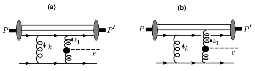
Figure 5: Valence quark description of proton where one (a) or two (b) quarks get hit by a gluon.

Let us first consider the process $pp\to ppH$, similar to the elastic cross section in Eq. (2.6). This involves two form factors corresponding to diagrams (5a) and (5b). One starts with a proton of momentum $\cal P$ and ends with an on-shell proton of momentum

$${\cal P}_{1}=x_{1}{\cal P}-{{\bf p}_{1}^{2}\over x_{1}s}{\cal P}^{\prime}+{\bf p}_{1}$$ (3.27)

${\cal P}^{\prime}$ is the momentum of the proton with three momentum opposite to that of ${\cal P}$. What matters for the quark recombination, and hence for the form factor, is the transverse kinematics in the ${\cal P}_{1}$ frame. The total momentum transfer is $\Delta={\cal P}_{1}-{\cal P}=k+k_{1}$, with

$$k = O(1/s){\cal P}+O(1/s){\cal P}^{\prime}+{\bf k}$$

$$k_{1} = (x_{1}-1){\cal P}+O(1/s){\cal P}^{\prime}+{\bf p}_{1}-{\bf k}$$ (3.28)

We want to calculate the transverse parts of the gluon momenta $k_{1}$ and $k$ w.r.t. the ${\cal P}_{1}$ direction. The momentum of the first gluon $k$ is purely transverse to order $1/s$ and does not directly enter into Higgs production. To order $1/s$ its transverse part remains unchanged. The momentum $k_{1}$ has a non-negligible component in the ${\cal P}$ direction. With respect to the ${\cal P}_{1}={\cal P}+k+k_{1}$ direction it becomes

$$k_{1} = ({x_{1}-1\over x_{1}})({\cal P}+k+k_{1})+{\tilde{\bf k}}_{1}+O(1/s)$$ (3.29)

where the vector ${\tilde{\bf k}}_{1}$ is now transverse to ${\cal P}_{1}$. Solving this equation for $k_{1}$ we get

$${k_{1}\over x_{1}}=(x_{1}-1){\cal P}+O(1/s){\cal P}^{\prime}+{x_{1}-1\over x_{1}}{\bf k}+{\tilde{\bf k}}_{1}$$ (3.30)

which by comparing to Eq. (3.28) gives:

$${\tilde{\bf k}}_{1}={{\bf p}_{1}-{\bf k}\over x_{1}}-{x_{1}-1\over x_{1}}{\bf k}={{\bf p}_{1}\over x_{1}}-{\bf k}$$ (3.31)

Hence, the transverse momenta which must enter the form factor are ${\bf k}$ and $\tilde{\bf k}_{1}$. We need to worry a little further as the coefficients of the dot products can also be $x_{1}$ dependent.

To check this, and to check how $x_{1}$ enters into the diagram, we consider the simplest case: the form factor ${\cal E}_{1}$ in the case of elastic of pion scattering. way is to consider ${\cal E}_{1}$ in the case of pion exchange.

First solve for the pion kinematics: let $\Delta=(x_{1}-1)\ {\cal P}+2\beta_{\Delta}/s\ {\cal P}^{\prime}+{\bf\Delta}$, with ${\cal P}.{\cal P}=0$, ${\cal P}^{\prime}.{\cal P}^{\prime}=0$ and ${\cal P}.{\cal P}^{\prime}=s/2$. The on-shell condition for the final pion, $({\cal P}+\Delta).({\cal P}+\Delta)=0$, gives:

$$\beta_{\Delta}=-{{\bf\Delta}^{2}\over 2\ x_{1}}$$ (3.32)

and the total momentum transfer squared is:

$$t={{\bf\Delta}^{2}\over x_{1}}=x_{1}(\tilde{\bf k}_{1}+\tilde{\bf k})$$ (3.33)

As we are calculating the imaginary part of the diagram, we have a few on-shell conditions for some of the quarks: one of the incoming quarks is on-shell, call its momentum $r$, with $r=x\ {\cal P}+2\beta_{r}/s\ {\cal P}^{\prime}+{\bf r}$. The on-shell condition $r.r=0$ gives

$$\beta_{r}=-{{\bf r}^{2}\over 2\ x}$$ (3.34)

The off-shellness of the other quark is:

$$m^{2}=({\cal P}-r).({\cal P}-r)={{\bf r}^{2}\over x}$$ (3.35)

The momentum of the first gluon is given by $k=2\alpha_{k}/s\ {\cal P}+2\beta_{k}/s\ {\cal P}^{\prime}+{\bf k}$, and the last on-shell condition, $({\cal P}-r+k).({\cal P}-r+k)=0$, gives:

$$\beta_{k}={{\bf k}^{2}\ x-2\ {\bf k}.{\bf r}\ x+{\bf r}^{2}\over 2\ x\ (x-1)}+O(1/s)$$ (3.36)

The second gluon is $k_{1}=\Delta-k$, with

$$k_{1}\approx(x_{1}-1)\ {\cal P}+{-2\ x_{1}\beta_{k}-x_{1}\ t\over x_{1}\ s}\ {\cal P}^{\prime}-{\bf k}+{\bf\Delta}$$ (3.37)

Now, the dot product of the two quarks making up the proton is:

$$A_{2}=2r.(p-r+\Delta)=-2(p-r+\Delta).(p-r+\Delta)={-m^{2}}x_{1}+2{\bf r}.{\bf\Delta}-x\ t$$ (3.38)

The form factor emerges as a convolution of wavefunctions. These can only depend on the dot products of the 2 quarks making the proton, hence on $A_{1}$ and $A_{2}$. In the case where $x_{1}=1$, one gets:

$$\int\psi^{*}({{\bf r}^{2}\over x})\psi({{\bf r}\over\sqrt{x}}-\sqrt{x}{\bf\Delta})^{2}d^{2}{\bf r}dx$$ (3.39)

which clearly is a function of $\bf\Delta$ only. In the more general case, one gets:

$$\int\psi^{*}({{\bf r}^{2}\over x})\psi({r\over\sqrt{x/x_{1}}}-\sqrt{x/x_{1}}{\bf\Delta})^{2}d^{2}{\bf r}dx$$ (3.40)

So, for $t_{1}>>m^{2}$, one gets $F_{1}(t_{1})$. However, this is not true in general, and the form factor clearly has an extra $x_{1}$ dependence: $\bf\Delta=0$ does not lead to a form factor equal to 1. One can in fact make a rough guess: the effective argument is $\tilde{t}=t+<{m^{2}\over x}>(1-x_{1})$ and $<{m^{2}\over x}>\approx 9\times 0.3^{2}\approx 1$ GeV².

Hence we see that the ansatz is as follows: replace the transverse vector ${\bf k}_{1}$ by $\tilde{\bf k}_{1}$, and multiply the overall argument by $x_{1}$. Note that this guarantees the infrared finiteness of the answer when $k^{2}$ or $k_{1}^{2}={\tilde{\bf k}}^{2}/x_{1}\rightarrow 0$. Clearly, this procedure straightforwardly generalises to the diffractive case $pp\to X_{1}X_{2}H$.

4. Higgs production

Apart from the form factors $W_{1}$ and $W_{2}$, the preceeding formalism can be applied to the production of any rare particle within a rapidity gap. We shall now specialise the calculation to the production of the minimal standard model Higgs boson. We first calculate the effective coupling resulting from the triangle graphs.

4.1. Higgs-gluon-gluon effective vertex

By calculating the diagrams in Fig. 6 we arrive at the following effective Higgs-gluon-gluon vertex:

$$\delta^{ab}(k_{1}\cdot k_{2}g^{\mu\nu}-k_{1}^{\mu}k_{2}^{\nu}){W_{1}\over m_{H}^{2}}+(k_{1}^{2}k_{2}^{2}g^{\mu\nu}+k_{1}^{\mu}k_{2}^{\nu}k_{1}\cdot k_{2}-k_{1}^{\mu}k_{1}^{\nu}k_{2}^{2}-k_{2}^{\mu}k_{2}^{\nu}k_{1}^{2}){W_{2}\over m_{H}^{4}}$$ (4.1)

where

$$W_{1}={[\sqrt{2}G_{f}]^{1/2}\alpha_{s}m_{H}^{2}\over 3\pi}N_{1}\qquad W_{2}={[\sqrt{2}G_{f}]^{1/2}\alpha_{s}m_{H}^{2}\over 3\pi}N_{2}$$ (4.2)

and

$$N_{1} = 3\int^{1}_{0}dx\int^{1-x}_{0}dy{1-4xy\over D}$$ (4.3)

$$N_{2} = {3m_{H}^{2}\over k_{1}\cdot k_{2}}\int^{1}_{0}dx\int^{1-x}_{0}dy{1-2x-2y+4xy\over D}$$ (4.4)

$$D \equiv 1-(2k_{1}\cdot k_{2}/m_{t}^{2})xy+(k_{1}^{2}/m_{t}^{2})(y^{2}-y)+(k_{2}^{2}/m_{t}^{2})(x^{2}-x)$$ (4.5)

Figure 6: The Higgs-gluon-gluon vertex. All quarks run around in the loop, but since the Higgs-quark-quark coupling is proportional to its mass, the top quark contribution dominates.

Because of the kinematics of Higgs production in a rapidity gap, $k_{1}^{2},k_{2}^{2}<<2k_{1}\cdot k_{2}\approx m_{H}^{2}$, and we can approximate the integral expression by setting $k_{1}^{2},k_{2}^{2}$ equal to zero:

$$N_{1}^{o} = 3\int^{1}_{0}dx\int^{1-x}_{0}dy{1-4xy\over D^{o}}$$ (4.6)

$$N_{2}^{o} = 6\int^{1}_{0}dx\int^{1-x}_{0}dy{1-2x-2y+4xy\over D^{o}}$$ (4.7)

$$D^{o} \equiv 1-(m_{H}^{2}/m_{t}^{2})xy-i\epsilon$$ (4.8)

Note that with $k_{1}^{2}$ and $k_{2}^{2}$ set equal to zero it is the $i\epsilon$ prescription coming from the top quark propagators in the loop that defines the contour.

Since the off-shellness of the gluons is small compared to the Higgs mass, and since the tensor structure (4.1) will always contract $k_{1}$ with the upper side ($\mu$) of the diagram and $k_{2}$ with the lower side ($\nu$), the $W_{2}$ term in Eq. (4.1) can be ignored, unless of course $|N^{o}_{2}|^{2}$ turns out to be abnormally large compared to $|N^{o}_{1}|^{2}$. As we explain in more detail in the Appendix, $|N^{o}_{2}|^{2}$ is always at least 30% smaller than $|N^{o}_{1}|^{2}$ for Higgs masses of 1 TeV or less. Thus we ignore $W_{2}$ and the above effective vertex can be derived from the following momentum space Lagrangian

$${\cal L_{\rm eff}}=A^{a}_{\mu}A_{a\nu}H(k_{1}\cdot k_{2}g^{\mu\nu}-k_{1}^{\mu}k_{2}^{\nu}){W_{1}\over m_{H}^{2}}$$ (4.9)

The term above, while not gauge invariant, forms part of the following gauge invariant term.

$${\cal L_{\rm eff}}={W_{1}\over 2m_{H}^{2}}G_{\mu\nu}^{a}G_{a\mu\nu}H$$ (4.10)

As a check we use our effective vertex to calculate the decay for $H\to gg$ and we obtain the well-known result

$$\Gamma(H\to gg)={|W_{1}|^{2}\over 2!\cdot 4\pi m_{H}}$$ (4.11)

where the last 2! is an identical final state particle phase space symmetry factor.

The approximate form of $N_{1}$ in Eq. (4.8) can be evaluated in closed form. Defining $a\equiv m_{H}^{2}/m_{t}^{2}$ we have

$$N_{1}^{o} = 3\int^{1}_{0}dx\int^{1-x}_{0}dy{1-4xy\over 1-axy-i\epsilon}$$

$$= {6\over a}\left[1-(1-4/a)\left(\arctan[\sqrt{a/(4-a)}]\right)^{2}\right]\qquad\quad{\rm if\ }a\equiv{m_{H}^{2}\over m_{t}^{2}}<4$$

$$= {6\over a}\left[1+(1-4/a)\left({\rm arctanh}[\sqrt{a/(a-4)}]\right)^{2}\right]\qquad\quad{\rm if\ }a\equiv{m_{H}^{2}\over m_{t}^{2}}>4$$

where ${\rm arctanh}(x)=\ln|(x+1)/(x-1)|-i\pi/2$. At $a=4$, $N^{o}_{1}=3/2$, and $N^{o}_{1}$ is continuous for the entire range of $a$. Note the change in sign in front of the second term between the two expressions.

4.2. The Higgs production cross section

From Eq. (3.2) we get:

$$\sigma={1\over\hat{s}^{3}}{(2/9)^{2}\over 8}{\alpha_{s}^{4}\over(2\pi)^{5}} \int{dx_{1}dy_{2}\over x_{1}y_{2}}{d^{2}{\bf p}_{1}d^{2}{\bf p}_{2}}d^{2}{\bf k}d^{2}{\bf K}\delta(H^{2}-M_{H}^{2})\tilde{\cal M}$$ (4.13)

$$3{\cal F}(k,k_{1},K_{1},K)~{}3{\cal F}(k,k_{2},K_{2},K)$$

with $k_{1}^{2}\approx({\bf k}+{\bf p}_{1})^{2}+(1-x_{1})({\bf k}^{2}-{\bf p}_{1}^{2})$, $k_{2}^{2}\approx({\bf k}+{\bf p}_{2})^{2}+(1-y_{2})({\bf k}^{2}-{\bf p}_{2}^{2})$, $k^{2}\approx{\bf k}^{2}$, and similar expressions for $K^{2}$, $K_{1}^{2}$, $K_{2}^{2}$, and the Higgs momentum

$$H^{2}=(p_{1}+p_{2}-p-p^{\prime})^{2}=\hat{s}(1-x_{1}+{{\bf p}_{2}^{2}\over\hat{s}y_{2}})(1-y_{2}+{{\bf p}_{1}^{2}\over\hat{s}x_{1}})+({\bf p}_{1}+{\bf p}_{2})^{2}$$ (4.14)

The form factors $3{\cal F}(k,k_{1},K_{1},K)~{}3{\cal F}(k,k_{2},K_{2},K)$ correspond to calculating the inelastic cross section $pp\rightarrow HX_{1}X_{2}$. To calculate $pp\rightarrow ppH$ these factors are replaced by an expression written in terms of the Dirac elastic form factor $F_{1}(t)$ given in Eq. (2.3)

$$(3F_{1}(t_{1})F_{1}(t_{2}))^{2}\qquad{\rm where}\quad t_{1}={{\bf p}_{1}^{2}/x_{1}}\quad{\rm and}\quad t_{2}={{\bf p}_{2}^{2}/y_{2}}$$ (4.15)

In order to make explicit the flat $s$ behaviour we first use Eq. (3.24) to substitute for $\tilde{\cal M}$

$$\sigma={\hat{s}\over 18}{\alpha_{s}^{4}\over(2\pi)^{5}} \int{dx_{1}dy_{2}\over x_{1}y_{2}}{d^{2}{\bf p}_{1}d^{2}{\bf p}_{2}}d^{2}{\bf k}d^{2}{\bf K}\delta(H^{2}-M_{H}^{2}){\cal A}W_{1}W_{1}^{\prime*}/m_{H}^{4}$$

$${\cal F}(k,k_{1},K_{1},K){\cal F}(k,k_{2},K_{2},K)D(k_{1}^{2})D(k_{2}^{2})D(k^{2})D(K_{1}^{2})D(K_{2}^{2})D(K^{2})$$

$\tilde{\cal M}$ brings in a factor of $\hat{s}^{4}$ and we still need a factor of $1/\hat{s}$ so we solve the Higgs momentum $\delta$ function for $x_{1}$ or $y_{2}$. (Note that scaling ${\bf p}_{1}$ and ${\bf p}_{2}$ by $\sqrt{s}$ produces the wrong power of $\hat{s}$.) In order to facilitate presenting the solution, we linearise the kinematics in terms of $1-y_{2}$. Hence

$$H^{2} \approx \hat{s}((1-x_{1})+{{\bf p}_{2}^{2}\over\hat{s}}+(1-y)2){{\bf p}_{1}^{2}\over\hat{s}})((1-y_{2})+{{\bf p}_{1}^{2}\over\hat{s}}+(1-x_{1}){{\bf p}_{1}^{2}\over\hat{s}})+({\bf p}_{1}+{\bf p}_{2})^{2}$$ (4.17)

$$\approx \hat{s}((1-x_{1})+{{\bf p}_{2}^{2}\over\hat{s}})((1-y_{2})+{{\bf p}_{1}^{2}\over\hat{s}})+({\bf p}_{1}+{\bf p}_{2})^{2}$$

Thus solving the $\delta$ function we get

$$1-y_{2}\equiv(1-y_{2})={M_{H}^{2}-({\bf p}_{1}+{\bf p}_{2})^{2}\over\hat{s}((1-x_{1})+{{\bf p}_{2}^{2}\over\hat{s}})}-{{\bf p}_{1}^{2}\over\hat{s}}$$ (4.18)

This brings a $1/\hat{s}/((1-x_{1})+{\bf p}_{2}^{2}/\hat{s})$ from the $\delta$ function upon performing the $dy_{2}$ integral and the answer behaves like $\hat{s}^{0}$.

There is an overall arbritrary angle in the integral with respect to which we measure all angles. We choose to measure our angles from ${\bf k}$. Thus $d^{2}{\bf k}=d\theta d{\bf k}^{2}/2=\pi d{\bf k}^{2}$. Thus we arrive at:

$$\sigma = {\alpha_{s}^{4}\over 18(2\pi)^{4}}\int dx_{1}~{}d{\bf k}~{}{d^{2}{\bf p}_{1}~{}d^{2}{\bf p}_{2}~{}}d^{2}{\bf K}~{}{1\over x_{1}y_{2}\left((1-x_{1})+{{\bf p}_{2}^{2}\over\hat{s}}\right)}$$

$$\times {\cal F}(k,k_{1},K_{1},K)\ {\cal F}(k,k_{2},K_{2},K)$$

$$\times D(k_{1}^{2})\ D(k_{2}^{2})\ D(k^{2})\ D(K_{1}^{2})\ D(K_{2}^{2})\ D(K^{2})$$

As explained in section 2, we need to multiply the above expression by a Regge factor, $\prod_{i=1,2}\left({s\over s_{i}}\right)^{\alpha(t_{1})}$, with $s_{i}=(p_{i}+H)^{2}$, and $t_{i}=(p-p_{i})^{2}$. This is our final expression for the cross section. Note that although the Regge factor is very important when one fits the purely soft cross sections (as in section 2.3), it plays very little role here, because $M_{H}^{2}$, and hence $s_{i}$ are sizeable fractions of $\hat{s}$.

4.3. The Bialas-Landshoff Limit

Bialas and Landshoff (BL) [10] work out the leading term in $(1-x_{1})$, $(1-y_{2})$ at ${\bf p}_{1}={\bf p}_{2}=0$, and then reintroduce the ${\bf p}_{1}$, ${\bf p}_{2}$ integration after reggeisation. In this limit, we get: $k_{1}^{2}=x_{1}{\bf k}^{2}$, $k_{2}^{2}=y_{2}{\bf k}^{2}$, ${\cal A}=(8\ |{\bf k}^{2}|W_{1})^{2}\hat{s}^{4}$. To compare more easily with BL, we do not eliminate the on-shell Higgs condition, and write:

$$d\sigma = {4\over 81\times 8\hat{s}}{\alpha_{s}^{4}\over(2\pi)^{5}\hat{s}^{3}}{dx_{1}\over x_{1}}{dy_{2}\over y_{2}}{d^{2}{\bf p}_{1}d^{2}{\bf p}_{2}}\delta((1-x_{1})(1-y_{2})-{M_{H}^{2}\over\hat{s}})$$ (4.20)

$$\times [\int d^{2}{\bf k}8\ |{\bf k}^{2}|D({\bf k}^{2})D(x_{1}{\bf k}^{2})D(y_{2}{\bf k}^{2})W_{1}]^{2}\hat{s}^{4}$$

$$= {\alpha_{s}^{4}\over 81\pi^{5}}{dx_{1}\over x_{1}}{dy_{2}\over y_{2}}{d^{2}{\bf p}_{1}d^{2}{\bf p}_{2}}\delta((1-x_{1})(1-y_{2})-{M_{H}^{2}\over\hat{s}})$$

$$\times [\int d^{2}{\bf k}\ |{\bf k}^{2}|D({\bf k}^{2})D(x_{1}{\bf k}^{2})D(y_{2}{\bf k}^{2})W_{1}]^{2}$$

which is identical to formula (4.2) in Ref. [10] at $\epsilon=\alpha^{\prime}=\lambda=0$, except for the factor of 2 which come from symmetrizing two identical particles as discussed in section 4.1.

Note that this is not the only simplification in their work, as they also assume that an exponentially falling propagator multiplying $F_{1}$ is a good representation of the product of the form factors by the gluon propagators. Furthermore, their estimate of the diffractive cross section comes from the replacement of $F_{1}$ by 1, and their integrals then converge only because of the Regge slope. We shall now see that, surprisingly, the improvements we have introduced – higher orders in $(1-x_{1})$, full form factors, propagators – do not significantly modify the final answer.

4.4. Results

Eq. (4.2.) is an eight-dimensional integral which we evaluate with the Monte-Carlo program VEGAS [22], both for the elastic cross section, $pp\to ppH$, (corresponding to using the form factors in Eqs. (2.7) and (2.11)), and for the diffractive cross section, $pp\to X\thinspace H$, (corresponding to the form factors described in Eq. (2.2.)).

Figure 7: The Higgs production cross section within a gap at 1.8 Tev

Figure 8: The Higgs production cross section within a gap at 10 TeV

Figure 9: The Higgs production cross section within a gap at 14 TeV

We present our results for the Tevatron ($\sqrt{s}=1.8$ TeV), and the LHC ($\sqrt{s}=10$ TeV and $\sqrt{s}=14$ TeV), in Figs. 7,8,9. The bands represent the effect of switching from a purely perturbative propagator to a renormalisation group improved propagator suppressed in the infrared region. We see that the extrapolation from the purely diffractive cross sections of section 2 to Higgs production seems to bring in relatively modest uncertainties of about a factor 2. The upper bands are for diffractive scattering, the lower bands for elastic scattering.

It is striking to note that our calculation leads to essentially the same conclusion as the Bialas-Landshoff estimate. This can be understood for the following reasons. One phenomenologically parametrises the model so as to correctly reproduce the soft elastic and diffractive cross sections. In the Higgs production diagrams, the off-shellness of the gluons is rather small $\mathrel{\raise 1.29167pt\hbox{$<$\kern-7.5pt\lower 4.30554pt\hbox{$\sim$}}}1$ GeV², and comparable to that in the soft diffractive processes which we fit to. The deep infrared region is cut off by the form factors. Thus the behaviour of the gluon propagator in the UV region and the deep IR region does not matter much, and the uncertainties arising from the extrapolation to Higgs production are small.

The diffractive cross section (upper band) is on average about a factor 5 higher than the elastic one (lower band). We call attention to the fact that it is really a factor 10 higher in the purely perturbative case, and a factor 3 higher if we use the constituent-gluon propagator. In other words the perturbative calculation is the upper limit of the diffractive band and the lower limit of the elastic band. Given the smallness of the gluon off-shellness, we consider the perturbative result less reliable.

We see that the cross section at the Tevatron is rather small, of the order of a fraction of a picobarn, for light Higgs masses. It indeed gets rapidly cut by the condition (3.20) which precludes production of particles of mass bigger than 200 GeV. If the Higgs is below 100 GeV, it will be observable within a rapidity gap at the Tevatron. A handful of them may already have been produced within the 60 pb^-1 available today.

Fig. 10 helps us understand the shape of the Higgs production curves, Figs. 7,8,9. Fig. 10a shows the vertex as a function of the Higgs mass. It rises with the Higgs mass, until one reaches the threshold for top quark production (after which the vertex is dominated by its imaginary part). Fig. 10b shows the $x_{1}$ distribution for a 100 GeV (solid line) and a 550 GeV Higgs (dashed line), in the diffractive case, for $\sqrt{s}=10$ TeV. Although the $x_{1}$ distribution is higher for the higher mass (because the vertex is bigger), it gets cut off at $x_{1}\approx 0.9$, after which one does not have enough partonic energy to produce a 550 GeV Higgs. Hence the low-mass Higgs cross section is higher because it is dominated by large $x_{1}$. This also shows that the dependence of the cross section on the cut-off $x_{1}>0.7$ (used to insure a rapidity gap) is very weak at low Higgs masses, and gets progressively larger as the cross section decreases: the main cause of its large fall-off at large Higgs masses is indeed the $x_{1}$ cut. Putting these considerations together we can understand the dip in the Higgs production curves before the rise peaking at about twice the top mass.

Figure 10: (a) The Higgs production vertex as defined by Eq. (4.1.). The thin solid line shows the real part, the dashed line the imaginary part, and the thick solid line the magnitude. (b) The $x_{1}$ distribution for a 100 GeV Higgs (solid line) and a 550 GeV Higgs (dashed line), for $\sqrt{s}=10$ TeV, in the diffractive case, using a constituent-gluon propagator.

Fig. 11 gives an estimate of the size of the rapidity gap. We show the rapidity distribution of the Higgs (thick solid line) and the partonic cluster (thin solid line). As the latter will fragment into hadrons, we envisage a worst case scenario, where the cluster decays into a forward proton and a backward pion. The dashed curves give the pion rapidity distributions. A gap is clearly present for $\sqrt{s}=10$ TeV, and the Higgs peak becomes sharper as the mass of the Higgs increases. At the Tevatron, we see that the gap is reduced to a few units of rapidity, but remains present.

Figure 11: The rapidity distribution of the Higgs (thick solid line), of the partonic cluster (thin solid line), and decay pions (dashed line) at (a) the LHC with $\sqrt{s}=10$ TeV and a 100 GeV Higgs (b) the LHC with $\sqrt{s}=10$ TeV and a 550 GeV Higgs (c) the Tevatron with a 100 GeV Higgs.

5. Conclusion and further studies

We have considered the lowest order QCD diagrams that give rise to Higgs production within a rapidity gap. They correspond to single pomeron exchange. We have found that the cross section is stable with respect to the details of the infrared region, and that it is a substantial fraction of the total Higgs production cross section this way at the Tevatron, whereas the LHC will comfortably produce 1 pb of 600 GeV Higgses within a gap.

There are three main factors effecting the accuracy of our predictions: the background, the survival of the gap, and higher order corrections. The first two effects will reduce our estimate, the last will increase it.

Although no conventional background is expected, there will be direct heavy quark production in the rapidity gap through the same color singlet exchange diagrams. Some work along this line [23] indicates that this background will be tiny for Higgs masses greater than 200 GeV. For Higgs masses less than 100 GeV the $c\bar{c}$ and $b\bar{b}$ background can be a problem.

Another issue to consider is the survival of the rapidity gap. Although the lowest order diagram produces a gap, further final-state interactions between the out-going partonic clusters might destroy it. Typical estimates for the survival of the gap give a number between 1 and 10% [24]. However, we want to point out that such an effect is implicitly included in our calculation: we fit the soft diffractive cross section, which already have to include such a survival factor, and as the kinematics of the event is not very different from the soft one, we expect those corrections to be small.

Finally, we have set up the calculation in such a way that higher orders can be calculated la BFKL [16]. In the elastic case these corrections dramatically increase the cross section (e.g. a factor of $\sqrt{s}/M_{H}$). We expect a similar effect in our calculation.

6. Appendix

In this Appendix we will justify neglecting the $W_{2}$ term in the effective vertex given in Eq. (4.1) when calculating Higgs boson production in a rapidity gap. Given the cuts we’ve imposed to insure the survival the gap, the approximate form of $N_{2}$ given in Eq. (4.8) can be used. Defining $a\equiv m_{H}^{2}/m_{t}^{2}$ we have

$$N_{2}^{o} = 6\int^{1}_{0}dx\int^{1-x}_{0}dy{1-2x-2y+4xy\over 1-axy-i\epsilon}$$ (6.3)

$$= {-12\over a}\left[5-(1+4/a)\left(\arctan[\sqrt{a/(4-a)}]\right)^{2}\right.$$

$$\left.~{}~{}~{}~{}~{}~{}~{}~{}~{}~{}~{}-{4\over\sqrt{a/(4-a)}}\arctan[\sqrt{a/(4-a)}]\right]~{}~{}~{}~{}~{}{\rm if\ }a\equiv{m_{H}^{2}\over m_{t}^{2}}<4$$

$$= {-12\over a}\left[5+(1+4/a)\left({\rm arctanh}\sqrt{a/(a-4)}\right)^{2}\right.$$

$$\left.~{}~{}~{}~{}~{}~{}~{}-{4\over\sqrt{a/(a-4)}}\left({\rm arctanh}\sqrt{a/(a-4)}\right)\right]{}~{}~{}~{}{\rm if\ }a\equiv{m_{H}^{2}\over m_{t}^{2}}>4$$

At $a=4$, $N^{o}_{2}=-15+3\pi^{2}/2$. It is the $i\epsilon$ prescription that tells us how to analytically continue from $a<4$ to $a>4$ by replacing

$$\sqrt{a\over 4-a} \rightarrow i\sqrt{a\over a-4}$$

$$\arctan\sqrt{a\over 4-a} \rightarrow i\left(\ln\left[{\sqrt{a/(a-4)}+1\over\sqrt{a/(a-4)}-1}\right]-i{\pi\over 2}\right)\equiv i\left({\rm arctanh}\sqrt{a\over a-4}\right)$$ (6.4)

We are interested in showing that the $N^{o}_{2}$ is never much greater than the $N^{o}_{1}$ term. The analytic expression for $N^{o}_{1}$ is given in Eq. (4.1.). We plot the ratio $|N^{o}_{2}|^{2}/|N^{o}_{1}|^{2}$ in Fig. 12 and see that it is always less than 0.30.

Figure 12: The ratio $|N^{o}_{2}|^{2}/|N^{o}_{1}|^{2}$ as a function of $a\equiv m_{H}^{2}/m_{t}^{2}$ between $a=0$ and $a=33$. With a top mass of $m_{t}=175$ GeV this corresponds to a Higgs mass $0<m_{H}<1$ TeV.

References

• [1] H1 Collaboration (T. Ahmed et al.) Nucl.Phys. B435 (1995);
ZEUS Collaboration (M. Derrick et al.), Phys. Lett. B346 (1995) 399.
• [2] J.D. Bjorken, Phys. Rev. D47 (1992) 101.
• [3] P. Giromini, in the Proceedings of the Vth Blois Workshop, Brown University, 8-12 June 1993 (World Scientific: Singapore, 1994), p. 30.
• [4] R. Rubinstein, in the Proceedings of the Vth Blois Workshop, Brown University, 8-12 June 1993 (World Scientific: Singapore, 1994), p. 23.
• [5] G. Ingelman and P.E. Schlein, Phys. Lett. 152B (1985) 256.
• [6] R. Bonino et al., Phys.Lett. 211B (1988) 239.
• [7] K. Goulianos, preprint RU-95-E-26 (May 1995), e-Print Archive: hep-ph/9505310.
• [8] J.F. Gunion and D. Soper, Phys. Rev. D 15 (1977) 2617
• [9] J.R. Cudell and B.U. Nguyen, Nucl.Phys. B420 (1994) 669.
• [10] A. Bialas and P.V. Landshoff, Phys. Lett.B256 (1991) 540.
• [11] A. Donnachie and P.V. Landshoff,  Nucl. Phys. B244 (1984) 322; B267 (1985) 690; Phys. Lett. B296 (1992) 227.
• [12] K. Goulianos, Phys. Rep. 101 (1983) 169.
• [13] A. Donnachie and P.V.Landshoff Phys. Lett. B296 (1992) 227.
• [14] F.E. Low, Phys. Rev. D12 (1975) 163; S. Nussinov, Phys. Rev. Lett. 34 (1976) 1286
• [15] E.M. Levin, M.G. Ryskin, Yad. Fiz. 34 (1981) 1114;
L.V. Gribov, E.M. Levin, M.G. Ryskin Phys. Rep. 100 (1983) 1.
• [16] E.A. Kuraev, L.N. Lipatov and V.S. Fadin,  Sov. Phys. JETP 45 (1977) 199
Y.Y. Balitskiǐ and L.N. Lipatov,  Sov. J. Nucl. Phys. 28 (1978) 822
• [17] P.V. Landshoff and O. Nachtmann,  Z. Phys. C35 (1987) 405.
• [18] K. Buttner and M.R. Pennington, preprint DTP-95-54, (June 1995), e-Print Archive: hep-ph/9506449.
• [19] J. R. Cudell and D.A. Ross,  Nucl. Phys. B359 (1991) 247
J.R. Cudell,  Proceedings of the $4^{th}$ Blois Workshop on Elastic & Diffractive Scattering, La Biodola, Italy (1991).
• [20] M.G. Ryskin, Sov.J.Nucl.Phys. 52 (1990) 529, Nuclear Physics B (Proc.Suppl.) 18C (1991) 162.
• [21] J.F. Gunion, H.E. Haber, G.L. Kane and S. Dawson, The Higgs Hunter’s guide, preprint SCIPP-89/13, June 1989, (Addison-Wesley, 1991); Errata, preprint SCIPP-92-58, Dec 1992, e-Print Archive: hep-ph/9302272.
• [22] G.P. Lepage, preprint CLNS-80/447 (March 1980).
• [23] A. Bialas and W. Szeremeta, Phys.Lett. B296 (1992) 191; W. Szeremeta, Acta Phys. Pol. B24 (1993) 1159.
• [24] R.S. Fletcher, Phys. Lett. B320 (1994) 373-376;
J.D. Bjorken (SLAC). SLAC-PUB-95-6949, Jul 1995;
E. Gotsman, E.M. Levin, U. Maor, Phys. Lett. B353 (1995) 526.