Almost-Goldstone Bosons from Extra-Dimensional
Gauge Theories

Abstract

A mechanism is presented through which very light scalar degrees of freedom obeying the nonlinear sigma model equation can emerge in spontaneously broken gauge theories. The mechanism operates in extra dimensional theories in which a) there are massless gauge fields present in the theory prior to compactification, and b) the extra dimensions are inhomogeneous in such a way that symmetry breaking Higgs fields aquire vevs only at very localised points on the manifold. These conditions are naturally fulfilled in orbifold compactifications of string theory. Possible applications include cosmic texture, axions and family symmetry.

Can the spontaneous breakdown of a gauge symmetry produce Goldstone bosons? In normal circumstances, the Higgs mechanism operates and the Goldstone bosons are ‘eaten’ by the longitudinal gauge bosons. In this Letter, however, I shall show that in modern approaches to theories with compact extra dimensions, the answer can be quite different. Under certain plausible conditions, very light modes remain which to all intents and purposes are the Goldstone bosons associated with the global part of the gauge symmetry. I call these modes almost-Goldstone bosons (AGB’s), because their mass is only exponentially small and not precisely zero.

Goldstone bosons and approximate Goldstone bosons are of considerable interest in cosmology, where they provide an attractive mechanisms for structure formation in the universe. A broken U(1) global symmetry produces cosmic strings [1], a broken nonabelian global symmetry produces cosmic texture [2]. In order for these structure formation mechanisms to work, it is essential for the Goldstone bosons extremely light, with mass no greater than $\sim 10^{-60}m_{Pl}$. Otherwise, the fields settle to their minimum and the field ordering process comes to an end, at a time of order their inverse mass. Similarly, the axion arises as an approximate Goldstone boson - in order for this mechanism to solve the strong CP problem, it is essential that any explicit mass term be very small, less than $\sim 10^{-38}m_{Pl}$. The reason for giving the number in Planck units will be made clear below. Finally, global continuous symmetries are of interest in the context of family symmetry ([3] and references therein).

Historically, the idea that there could be fundamental global symmetries has been unpopular in particle theory. The gauge principle is believed to be a ‘deeper’ idea. Dynamical theories of the origin of internal symmetries, such as string theory, naturally produce symmetries which are gauged [4]. Those global internal symmetries which are present in the standard model (related to baryon and lepton number conservation) may be explained as being simply ‘accidents’ of the gauge symmetry and particle content, which could not in general be expected to survive in larger unified schemes. And finally, it has been argued that quantum gravitational effects could ‘spoil’ global symmetries by introducing terms involving the Planck mass $m_{Pl}$ into the low energy effective theory which violate global symmetries in an arbitrary manner [5, 6]. These last arguments have to some extent been countered in [7].

Without getting into such arguments, it is still interesting to ask the following. If we do accept the proposition that at a fundamental level all internal symmetries are gauged, does it follow that Goldstone bosons of the kind that are interesting for cosmology are disallowed? I shall show that the answer is negative. In particular, if we start with an extra dimensional gauge theory with spontaneous symmetry breaking, under certain conditions AGB’s with exponentially small masses are produced. In a compactified field theory, one finds $m_{AGB}\propto e^{-ML}$, with $M$ a mass scale associated with the symmetry breaking Higgs field and $L$ the size of the extra dimensions. And in compactifications of string theory, the suppression can be even stronger - potentially, one has $m_{AGB}\propto e^{-TL^{2}}$ where $T$ is the string tension.

I shall assume that there exist gauge bosons before the theory is compactified, and that the extra dimensions do not possess any special continuous symmetry. Both assumptions are those usually made in modern approaches to Kaluza-Klein theory and string theory.

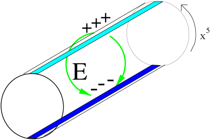
FIG. 1.: An example of symmetry breaking which is inhomogeneous in the extra dimensions, parametrised by $x^{5}$. The direction along the tube is an uncompactified dimension. The Higgs vev is large on the two shaded strips. A TEM mode can propagate along the tube, with a positive charge wavepacket travelling along one strip, a negative charge wavepacket along the other. E denotes the electric field.

As an illustration of the idea, consider compactification on a circle of length $L$. As mentioned above, I am really interested in the case where the extra dimensions do not possess any special symmetries. Therefore I shall ignore any effects due to the translational symmetry of the circle. Consider the abelian Higgs model in five dimensions, and assume that the Higgs field $\varphi$ gets a vev in the ground state which is inhomogeneous on the circle (Figure 1). Let me emphasise that I am just putting this vev in by hand in this example. The most natural origin for this inhomogeneity would be the inhomogeneity of the compactified dimensions, which requires more than one dimension, and is therefore harder to picture. For example in orbifold compactifications the curvature has delta function singularities at the fixed points of the orbifold. If $\varphi$ couples to the curvature in such a way that its effective mass squared is large and negative at these points, but positive elsewhere, it will aquire an inhomogeneous vev over the extra dimensions, with exponentially small values where its mass squared is positive.

The existence of a very light mode follows from the fact that the two strips of nonzero Higgs vev are superconducting wires, and the configuration shown is a transmission line. In Lorentz gauge, the equation of motion for the gauge field is

$$\partial^{2}A_{\hat{\mu}}=(\Box-\partial_{5}^{2})A_{\hat{\mu}}=-gv^{2}(x^{5})(\partial_{\hat{\mu}}\theta+gA_{\hat{\mu}})\equiv J_{\hat{\mu}}(x)$$ (1)

where $\partial^{2}$ is the full Laplacian, $\Box$ that for the uncompactified dimensions, and $\partial_{5}=\partial/\partial x^{5}$. Hatted indices run over all dimensions, unhatted indices over $0-3$. The phase $\theta$ is the phase of the Higgs field, and $g$ the gauge coupling constant. The Higgs vev $v(x^{5})$ is treated as fixed: we ignore the zero modes corresponding to translation of the wires around the extra dimensions, a result of the translational symmetry of the circle.

In the approximation that the wires are infinitely thin, $v^{2}(x^{5})=V^{2}\sum_{i}\delta(x^{5}-x_{i})$, and we can safely take the current $J_{5}$ flowing around the circle to be zero. We define the Higgs field phase on each wire to be $\theta^{(i)}$, $i=1,2$, and seek a solution in which $A_{5}$ is zero, but $A_{\mu}=f(x^{5})a_{\mu}(x^{\alpha})$. The form of $f(x^{5})$ is simple: between the wires it is linear in $x^{5}$, with slope $\pm f_{0}$. Note that $f(x^{5})$ must be periodic in $x^{5}$. This follows because we assume that the Higgs field has no winding number around the extra dimensions, so $\theta$ is single valued. But the currents $J_{\mu}$ must be single valued, and therefore so must $A_{\mu}$ be. Matching the slope discontinuity across each wire, using (1) we find $2f_{0}a_{\mu}(x^{\alpha})=gV^{2}(\partial_{\mu}\theta^{(1)}-{1\over 4}gLf_{0}a_{\mu})$, and similarly with $\theta^{(1)}$ replaced by $-\theta^{(2)}$. These equations require that $\partial_{\mu}\theta^{(1)}=-\partial_{\mu}\theta^{(2)}$. Thus we find

$$gA^{(1)}_{\mu}=-{I\partial_{\mu}\theta^{(1)}(x^{\alpha})\over(1+I)}=-gA^{(2)}_{\mu}$$ (2)

where $I={1\over 8}g^{2}LV^{2}$, and the current flowing on the two wires is

$$J^{(1)}_{\mu}={gV^{2}\partial_{\mu}\theta^{(1)}\over(1+I)}=-J^{(2)}_{\mu}.$$ (3)

The solution to these equations involves one massless scalar degree of freedom, $\theta(x^{\alpha})$, obeying the equation for current conservation, $\Box\theta=0$. It describes the propagation of a transverse electromagnetic field (TEM) mode down the transmission line provided by the extra dimensions. Just as in a transmission line, we need at least two wires to carry the light mode. It is straightforward to find all the propagating modes, and to show that they have masses $\sim L^{-2}$, the usual Kaluza-Klein tower of massive states.

One simple way of understanding the mechanism is to realise that before the symmetry is gauged, the phases of the Higgs field on the two wires, $\theta^{(1)}$ and $\theta^{(2)}$, are decoupled in the limit that $v(x^{5})$ vanishes in between the wires. Thus there are actually two four-dimensional Goldstone modes. When the gauge field is introduced, it can only ‘eat’ one of these (the linear combination $\theta^{(1)}+\theta^{(2)}$), leaving the other massless. The extra dimensions can produce more than one, and in principle an infinity of four-dimensional Goldstone modes, and thereby ‘evade’ the Higgs mechanism.

This discussion generalises to the nonabelian case quite straightforwardly. The key point is that the only large [8] components of the electromagnetic field tensor are $F_{50}$ and $F_{5i}$. Since $A_{5}$ is zero, neither of these involves any commutator terms, and the equations of motion are the same as in the abelian case, (1), with an extra Lie algebra-valued index on the gauge fields and scalar field current $J_{\mu}$. Apart from adding the extra indices, the change in the formulae (2) and (3) is that $\partial_{\mu}\theta$ is replaced by $-i$ Im($\varphi^{\dagger}T^{a}\partial_{\mu}\varphi)/v^{2}$, where $T^{a}$ are the generators of the gauge group. In the approximation that all massive modes are set zero, conservation of this current is equivalent to the nonlinear sigma model (NLSM) equation.

This is an important point. In the abelian case, the compactified theory already has a massless scalar, before symmetry breaking, namely $A_{5}(x^{\alpha})$. So it might appear that all we have done is to relabel this mode in a way that makes it look like a Goldstone boson. The nonabelian case demonstrates that this is not so - the field equation describing the low energy excitations really is the NLSM equation, whereas for a dimensionally reduced nonabelian gauge theory $A^{a}_{5}(x^{\alpha})$ is instead a massless scalar field in the adjoint representation of the gauge group.

We now have all the ingredients needed for the cosmological structure formation mechanism. We assume as usual that the Higgs vev $<\varphi>$ is zero at high temperatures, and a symmetry breaking occurs as the universe cools. The Higgs field aquires an orientation in internal space which is uncorrelated on large (three-dimensional) spatial scales. Then ordering of the fields proceeds, just as in the usual scenario [1, 2]. Fluctuations of the observed amplitude are produced for $V\sim 10^{-3}m_{Pl}$.

We now turn to a more realistic computation, where we include the dynamics producing the inhomogeneous Higgs vev. In this case, we shall find that the mode described above gets an exponentially small mass. To be specific, consider the case where a charged scalar field $\varphi$ has a coupling to the Ricci curvature $R$, of the form $\xi R\varphi^{\dagger}\varphi$, with the sign such as to give $\varphi$ a large negative mass squared at special locations on the extra dimensions. Let us make the approximation that the scalar curvature $R$ has delta function singularities in the extra dimensions. The simplest example would be two extra dimensions taking the form of a narrow tube with rounded ends, with strong curvature at either end and none in between. Note that whatever the sign of $\xi$ there is always some form for the extra dimensions which will produce the negative mass squared: for example, by adding a small handle to each end of the rounded tube just mentioned, one can make the Euler number negative so that the mean curvature at each end will be large and negative [9].

The equation we need to solve for the value of the symmetry breaking field in the ground state, $\varphi^{\dagger}\varphi=v^{2}(x^{5})$ is:

$$-\partial_{5}^{2}v=-\lambda v^{3}-m^{2}v+\xi\sum_{i}\delta(x^{5}-x^{i})v(x^{i}).$$ (4)

The symmetry breaking field is assumed to have a positive mass squared term and a quartic term in its potential. The solution to (4) describes a particle rolling up one side of the ‘upside down’ potential, approaching the ‘summit’ slowly before turning around and descending again. The delta function terms reverse the ‘velocity’ $\partial_{5}v$, sending $v$ rolling back up the hill. If we assume that the size $L$ of the circle is large, then $v(x^{5})$ becomes nearly zero in between the delta functions. Then the value of $v$ at the delta functions is determined by energy conservation, ${1\over 2}(\partial_{5}v)_{max}^{2}\approx{1\over 4}\lambda v_{max}^{4}+{1\over 2}m^{2}v_{max}^{2}$, and the matching condition $2\partial_{5}v_{max}=\xi v_{max}$. Thus we find $v_{max}^{2}=(\xi^{2}-4m^{2})/2\lambda$. A nonzero solution exists if $\xi>2m$, which is just the condition for instability of the configuration $v(x^{5})=0$. In between the delta functions, $v$ gets exponentially small, $v_{min}\sim e^{-Lm/4}$. So the symmetry breaking is exponentially small, but nonzero, in between the wires.

We would now like to determine the mass of the lightest mode in this more realistic setting. The calculation is most easily done in unitary gauge, which is adequate for considering small fluctuations about the ground state. In fact, it is interesting to see exactly how the light mode emerges here, because in this gauge there are no degrees of freedom associated with the phases of the Higgs field. Instead we just have a single massive vector boson. Its equation of motion is

$$\partial_{\hat{\mu}}F^{\hat{\mu}\hat{\nu}}=-M^{2}(x^{5})A^{\hat{\nu}}$$ (5)

where $M^{2}=g^{2}v^{2}$. This equation implies that $\partial_{\hat{\mu}}(M^{2}(x^{5})A^{\hat{\mu}})=0$, and solving for $\partial_{\hat{\mu}}A^{\hat{\mu}}$ one finds

$$-\Box A_{\hat{\mu}}=(-\partial_{5}^{2}+M^{2}(x^{5}))A_{\hat{\mu}}-\partial_{\hat{\mu}}({\partial_{5}M^{2}\over M^{2}}A_{5})$$ (6)

For $\hat{\mu}=5$, this only involves $A_{5}$. The right-hand side is a linear operator $\hat{O}$ acting on $A_{5}$: the eigenvalues of $\hat{O}$ are the squared masses $M_{4}^{2}$ of the four-dimensional fields corresponding to $A_{5}$.

The operator $\hat{O}$ can be replaced by a hermitian operator $\hat{H}$ if we remove the first order derivative by redefining $A_{5}=a(x^{5})/M(x^{5})$. One finds $\hat{H}=\hat{H}_{1}+M^{2}$, where $\hat{H}_{1}=-\partial_{5}^{2}+M\partial_{5}^{2}(M^{-1})$. Now a minor miracle happens: $\hat{H}_{1}$ has an eigenvalue which is exactly zero, with eigenfunction $a(x^{5})=M^{-1}(x^{5})$, localised in between the wires. We obtain a useful upper bound on the mass squared of the lightest four-dimensional mode by simply using this zero mode of $\hat{H}_{1}$ as a trial function:

$$M_{4}^{2}<{\int dx^{5}(a\hat{H}a)\over\int dx^{5}a^{2}}={L\over\int dx^{5}M^{-2}(x^{5})}.$$ (7)

But this means that $M_{4}^{2}$ is very small, because the integral in the denominator has an exponentially large contribution in between the wires, where the gauge boson mass $M(x^{5})$ becomes small. The mass of the lightest mode is suppressed as $e^{-Lm/4}$, as claimed above.

The mechanism discussed above seems to work even more efficiently in string theory. The natural analogs of the curvature-coupled Higgs field are the so-called twisted modes on orbifolds [10], which play a central role in string phenomenology. Viewed as modes of the string these excitations have a center of mass which cannot propagate on the orbifold, they are literally stuck on the orbifold fixed points. There is nothing preventing the scalar fields corresponding to these twisted modes aquiring a GUT-scale vev, and the interactions between the modes associated with different fixed points are all exponentially suppressed.

Some couplings are suppressed by a Gaussian rather than an exponential in the distance between the fixed points. This can be heuristically understood as follows. In order for twisted string modes at two different fixed points to interact, they must undergo a large quantum fluctuation, in which their size changes by a scale of order the distance $L$ between the fixed points. Such fluctuations are suppressed by the large Euclidean action involved, the area of the string worldsheet times the string tension. Since the string dynamics is independent of the tension $T$, dimensional analysis indicates the action must be proportional to $L^{2}$. The suppression factor is therefore $\sim e^{-TL^{2}}$. The exponent has been calculated in some explicit examples by Hamidi and Vafa [11], and by Dixon, Friedan, Martinec and Shenker[12]. So if $L$ is of order ten or twenty string units, the coupling is completely negligible.

The field theory form of the exponential suppression may also occur here [13]. For example, on a $Z_{N}$ orbifold $N$ identical twisted strings may combine at a fixed point into an untwisted state, carrying gauge group indices for the symmetric product representation, which can then propagate across to a neighbouring fixed point. In this case it is natural to conjecture the suppression would instead be $\sim e^{-ML}$, with $M$ the mass of the intermediate untwisted charged state, and $L$ the distance between fixed points. Again, in string theory the prospect of obtaining a large exponent is better than in field theory because the intermediate state could be forced to be a high level number massive string mode. As a quasi-realistic example, the $Z_{3}$ orbifold [10] has massless gauge fields corresponding to the gauge group $E_{6}\times SU(3)$, and there are no less than eighty one $(\bf{1},\bf{3})$’s (three at each fixed point). There is certainly no shortage of candidate fields for forming $SU(3)$ global texture in this model. Indeed one might instead worry that too many light AGB’s might be produced, thus causing conflict with primordial nucleosynthesis.

What are the limits to the exponential suppression? There is a well-known problem associated with making the extra dimensions very large, namely that in dimensional reduction, the higher dimensional gauge coupling gets large, $\alpha=\alpha_{4}{\cal V}$ where ${\cal V}$ is the volume of the compactified space, and $\alpha$ as usual is $g^{2}/4\pi$. If ${\cal V}$ increases too far, then for fixed four-dimensional coupling the higher dimensional theory is in the strong coupling limit, and calculations are impossible. As a simple example, consider an orbifold, with all dimensions small except one. The five dimensional coupling would then be potentially problematic. Let us estimate the largest possible suppression factor $e^{-ML}$, following the discussion of the previous paragraph. Here $L=\alpha_{5}/\alpha_{4}$, and we could consider taking the dimensionless loop expansion parameter $(\pi T)^{1\over 2}\alpha_{5}/(2\pi)$ to be of order unity. We use $\alpha_{4}=1/27$, the GUT coupling, and for $M$ take the mass of a massive string intermediate state, $M=\sqrt{8\pi Tn}$ with $n$ the level number (for closed strings). The suppression factor is then $\sim e^{-480\sqrt{n}}$!

One should also note that that there are other strong constraints on twisted mode couplings and in general higher powers of the exponential suppression factors can be involved. This discussion I have presented is of course very preliminary, one should aim at a general statement about the precise form of the suppression in an arbitrary term in the full effective potential. However, I hope I have succeeded at least in emphasising that that numerical factors of $2\pi$ are important in exponents, and that a detailed study would be worthwhile.

The above considerations may be summarised by saying that compactified extra dimensions can provide a physical reason for the existence of several global copies of the original gauge group in the effective four-dimensional theory. Applications of this idea to realistic orbifold models of cosmic texture, axions and family symmetry are interesting directions for future work.

I thank M. Bucher, A. Farraggi, A. Goldhaber, D. Gross, H. Verlinde, F. Wilczek, E. Witten and especially L. Dixon for very helpful discussions. This work was partially supported by NSF contract PHY90-21984, and the David and Lucile Packard Foundation.

REFERENCES

- [1] For a review see A. Vilenkin and E.P.S. Shellard, Cosmic Strings and other Topological Defects, CUP (1994).
- [2] N. Turok, Phys. Rev. Lett. 63 (1989) 2625.
- [3] M. Joyce and N. Turok, Nuc. Phys. B416, 389 (1994).
- [4] T. Banks and L. Dixon, Nuc. Phys. B307, 93 (1988).
- [5] S. Giddings and A. Strominger, Nuc. Phys. B306, 890 (1988).
- [6] R. Holman et. al., Phys. Rev. Lett. 69, 1489 (1992) and M. Kamionkowski and J. March-Russell, Phys. Rev. Lett. 69, 148 (1992).
- [7] R. Kallosh, A. Linde, D. Linde and L. Susskind, preprint SU-ITP-95-2, hep-th/9502069 (1995).
- [8] There is in this case a nonzero contribution to , but this is down by where is the wavelength of the four-dimensional mode. A more detailed analysis (N. Turok, to appear) reveals that the nonlinear sigma model that arises has an infinite series of higher derivative couplings, just in the chiral model description of the strong interactions. It is interesting that in the present context this series is exactly calculable from the classical field theory.
- [9] Inhomogeneity of the extra dimensions is generic to solutions in superstring and supergravity theory. However, there is at present only an incomplete understanding of what fixes the size and shape of the extra dimensions.
- [10] L. Dixon, J. Harvey, C. Vafa and E. Witten, Nuc. Phys. B261, 678 (1985); B274, 285 (1986).
- [11] S. Hamidi and C. Vafa, Nuc. Phys. B279, 465 (1987).
- [12] L. Dixon, D. Friedan, E. Martinec and S. Shenker, Nuc. Phys. B279, 465 (1987).
- [13] This picture was developed in conversations with L. Dixon.