Collision Induced Decays of Electroweak Solitons:
Fermion Number Violation with Two and Few Initial Particles

Abstract

We consider a variant of the standard electroweak theory in which the Higgs sector has been modified so that there is a classically stable weak scale soliton. We explore fermion number violating processes which involve soliton decay. A soliton can decay by tunnelling under the sphaleron barrier, or the decay can be collision induced if the energy is sufficient for the barrier to be traversed. We present a classical solution to the Minkowski space equations of motion in which a soliton is kicked over the barrier by an incoming pulse. This pulse corresponds to a quantum coherent state with mean number of $W$ quanta $\sim 2.5/g^{2}$ where $g$ is the $SU(2)$ gauge coupling constant. We also give a self-contained treatment of the relationship between classical solutions, including those in which solitons are destroyed, and tree-level quantum amplitudes. Furthermore, we consider a limit in which we can reliably estimate the amplitude for soliton decay induced by collision with a single $W$-boson. This amplitude depends on $g$ like $\exp(-cg^{-1/3})$, and is larger than that for spontaneous decay via tunnelling in the same limit. Finally we show that in soliton decays, light $SU(2)_{L}$ doublet fermions are anomalously produced. Thus we have a calculation of a two body process with energy above the sphaleron barrier in which fermion number is violated.

CTP#2483

HUTP-95-A039 Submitted to Physical Review D

hep-ph/9511219 Typeset in REVTeX

I Introduction

In the standard electroweak theory, fermion number violation is present at the quantum level but these processes are seen only outside of ordinary perturbation theory. A baryon number three nucleus can decay into three leptons. The process is described as an instanton mediated tunnelling event[1] leading to an amplitude which is suppressed by $\exp(-8\pi^{2}/g^{2})$, with $g\simeq 0.65$ the $SU(2)$ gauge coupling constant. At energies above the sphaleron barrier[2], fermion number violating processes involving two particles in the initial state are generally believed to be also exponentially suppressed[3]. (At energies comparable to but below the sphaleron barrier, Euclidean methods[4] have been used to show that the exponential suppression is less acute than at lower energies, but the approximations used fail at energies of order the barrier height and above.) Unsuppressed fermion number violating processes are generally believed to have of order $4\pi/g^{2}$ particles in both the initial and final states. This all suggests that fermion number violation will remain unobservable at future accelerators no matter how high the energy, whereas in the high temperature environment of the early universe such processes did play a significant role[5].

In this paper, we explore the robustness of these ideas by studying a variant of the standard model in which the amplitudes for certain fermion number violating collisions, as well as for spontaneous decays, can be reliably estimated for small coupling $g$. The model is the standard electroweak theory with the Higgs mass taken to infinity and with a Skyrme term[6] added to the Higgs sector. With these modifications, the Higgs sector supports a classically stable soliton which can be interpreted as a particle whose mass is of order the weak scale[7]. Quantum mechanically, the soliton can decay via barrier penetration[8, 9, 10]. Classically, i.e., evolving in Minkowski space using the Euler-Lagrange equations, the soliton can be kicked over the barrier if it is hit with an appropriate gauge field pulse. Correspondingly, the soliton can be induced to decay quantum mechanically if it absorbs the right gauge field quanta. Regardless of whether the decay is spontaneous or induced, ordinary baryon and lepton number are violated in the decay. We shall see that the model has a limit in which fermion number violating amplitudes can be reliably estimated both for processes which occur by tunnelling and for those which occur in two particle collisions between a soliton and a single $W$-boson with energy above the barrier.

A The Model

To modify the standard model so that it supports solitons, proceed as follows. Note that in the absence of gauge couplings the Higgs sector can be written as a linear sigma model

$${\cal L}_{\rm H}=\frac{1}{2}\,{\rm Tr}\left[\partial_{\mu}\Phi^{\dagger}\partial^{\mu}\Phi\right]-\frac{\lambda}{4}\left({\rm Tr}\left[\Phi^{\dagger}\Phi\right]-v^{2}\right)^{2}$$ (1)

where

$$\Phi({\bf x},t)=\left(\matrix{\varphi_{0}&-\varphi_{1}^{*}\cr\varphi_{1}&\varphi_{0}^{*}}\right)\ ,$$ (2)

$(\varphi_{0},\varphi_{1})$ is the Higgs doublet, and $v=246~{}{\rm GeV}$. One advantage of writing the Lagrangian in this form is that it makes the $SU(2)_{L}\times SU(2)_{R}$ invariance of the Higgs sector manifest. The scalar field $\Phi$ can also be written as

$$\Phi=\sigma\,U$$ (3)

where $U$ is $SU(2)$ valued and $\sigma$ is a real field. In terms of these variables

$${\cal L}_{\rm H}=\frac{1}{2}\,\sigma^{2}\,{\rm Tr}\left[\partial_{\mu}U^{\dagger}\partial^{\mu}U\right]+\partial_{\mu}\sigma\partial^{\mu}\sigma-\lambda\left(\sigma^{2}-\frac{v^{2}}{2}\right)^{2}\ .$$ (4)

The Higgs boson mass is $\sqrt{2\lambda}v$. We work in the limit where the Higgs mass is set to infinity and $\sigma$ is frozen at its vacuum expectation value $v/\sqrt{2}$. Now

$${\cal L}_{H}=\frac{v^{2}}{4}{\rm Tr}\left[\partial_{\mu}U^{\dagger}\partial^{\mu}U\right]$$ (5)

which is the nonlinear sigma model with scale factor $v$. We will consider only those configurations for which the fields approach their vacuum values as $|{\bf x}|\rightarrow\infty$ for all $t$. We can then impose the boundary condition

$$\lim_{|{\bf x}|\rightarrow\infty}U({\bf x},t)=1\ ,$$ (6)

which means that at any fixed time $U$ is a map from $S^{3}$ into $SU(2)$. These maps are characterized by an integer valued winding number which is conserved as the $U$ field evolves continuously. However if we take a localized winding number one configuration and let it evolve according to the classical equations of motion obtained from (5) it will shrink to zero size. To prevent this we follow Skyrme[6] and add a four derivative term to the Lagrangian. The Skyrme term is the unique Lorentz invariant, $SU(2)_{L}\times SU(2)_{R}$ invariant term which leads to only second order time derivatives in the equations of motion and contributes positively to the energy.

$${\cal L}_{H\&S}=\frac{v^{2}}{4}{\rm Tr}\left[\partial_{\mu}U^{\dagger}\partial^{\mu}U\right]+\frac{1}{32e^{2}}{\rm Tr}\left[U^{\dagger}\partial_{\mu}U\,,\,U^{\dagger}\partial_{\nu}U\right]^{2}$$ (7)

where $e$ is a dimensionless constant.

Of course this Lagrangian is just a scaled up version of the Skyrme Lagrangian which has been used[6, 11, 12] to treat baryons as stable solitons in the nonlinear sigma model theory of pions. To obtain the original Skyrme Lagrangian replace $v$ in (7) by $f_{\pi}=93{\rm~{}MeV}$. The stable soliton of this theory, the skyrmion, has a mass of $73\,f_{\pi}/e$ and has a size $\sim 2/(ef_{\pi})$[12]. Best fits to a variety of hadron properties give $e=5.5$[12]. The soliton of (7) has mass $73\,v/e$ and size $\sim 2/(ev)$ and we take $e$ as a free parameter since the particles corresponding to this soliton have not yet been discovered.

The standard electroweak Higgs plus gauge boson sector is obtained by gauging the $SU(2)_{L}\times U(1)_{Y}$ subgroup of $SU(2)_{L}\times SU(2)_{R}$ in the Lagrangian (1). Throughout this paper we neglect the $U(1)$ interactions. The complete Lagrangian we consider is obtained upon gauging the $SU(2)_{L}$ symmetry of (7):

$${\cal L}=-\,\frac{1}{2g^{2}}\,{\rm Tr}F^{\mu\nu}F_{\mu\nu}+\frac{v^{2}}{4}\,{\rm Tr}\left[D^{\mu}U^{\dagger}D_{\mu}U\right]+\frac{1}{32e^{2}}\,{\rm Tr}\left[U^{\dagger}D_{\mu}U\,,\,U^{\dagger}D_{\nu}U\right]^{2}$$ (8)

where

$$F_{\mu\nu} = \partial_{\mu}A_{\nu}-\partial_{\nu}A_{\mu}-i[A_{\mu},A_{\nu}]$$ (9)

$$D_{\mu}\,U = (\partial_{\mu}-iA_{\mu})\,U$$ (10)

with $A_{\mu}=A_{\mu}^{a}\sigma^{a}/2$ where the $\sigma^{a}$ are the Pauli matrices. In the unitary gauge, $U=1$, and the Lagrangian is

$${\cal L}=\frac{1}{g^{2}}\left\{-\,\frac{1}{2}\,{\rm Tr}\,F^{\mu\nu}F_{\mu\nu}+m^{2}\,{\rm Tr}A_{\mu}A^{\mu}+\frac{1}{8\xi}\,{\rm Tr}\left[A_{\mu}\,,\,A_{\nu}\right]^{2}\right\}\ ,$$ (11)

where we have introduced

$$m=\frac{gv}{2}{\rm~{}~{}~{}and~{}~{}~{}}\xi=\frac{4e^{2}}{g^{2}}\ .$$ (12)

Note that the equations of motion derived from (11) agree with those obtained by varying (8) and then setting $U=1$. Also note that for fixed $m$ and $\xi$ the classical equations of motion are independent of $g$. Since $m$ is dimensionful and sets the scale, characteristics of the classical theory depend only on the single dimensionless parameter $\xi$.

B The Soliton and the Sphaleron

The classical lowest energy configuration of (11) has $A_{\mu}=0$ and the quantum theory built upon this configuration has three spin-one bosons of equal mass $m$. In the limit where $g$ goes to zero with $e$ and $v$ fixed (hence, $\xi$ goes to infinity) the Lagrangian (8) is well approximated by its ungauged version (7) which supports a stable soliton, so one suspects that for large $\xi$ the Lagrangian (8) and its gauge-fixed equivalent (11) also support a soliton. In fact, Ambjorn and Rubakov[10] showed that for $\xi$ larger than $\xi^{*}=10.35$ the Lagrangian (11) does support a classically stable soliton whereas for $\xi<\xi^{*}$ such a configuration is unstable. Let $U_{1}({\bf x})$ be the winding number one soliton, the skyrmion, associated with the ungauged Lagrangian (7). For large $\xi$, this configuration is a good approximation to the soliton of the gauged Lagrangian (8), so in the unitary gauge the soliton is $A^{\rm sol}_{i}\simeq i\,U_{1}^{\dagger}\partial_{i}U_{1}$, $A^{\rm sol}_{0}=0$. For all $\xi>\xi^{*}$ the quantum version of the theory described by (11) has, in addition to the three equal mass $W$-bosons, a tower of particles which arise as quantum excitations about the soliton, just as the proton, neutron and delta can be viewed as quantum excitations about the original skyrmion[11, 12].

The Lagrangian (11) determines a potential energy functional which depends on the configuration $A_{\mu}({\bf x})$. The absolute minimum of the energy functional is at $A_{\mu}=0$. For $\xi>\xi^{*}$ there is a local minimum at the soliton $A_{\mu}=A_{\mu}^{\rm sol}({\bf x})$ with nonzero energy given by the soliton mass $M_{\rm sol}$. (Of course a translation or rotation of $A_{\mu}^{\rm sol}({\bf x})$ produces a configuration with the same energy so we imagine identifying these configurations so that the soliton can be viewed as a single point in configuration space.) Consider a path in configuration space from $A_{\mu}=0$ to $A_{\mu}^{\rm sol}({\bf x})$. The energy functional along this path has a maximum which is greater than the soliton mass. As we vary the path, the maximum varies, and the minimum over all paths of this maximum is a static unstable solution to the classical equations of motion which we call the sphaleron of this theory. (The sphaleron of the standard model[2] marks the lowest point on the barrier separating vacua with different winding numbers. Here, the sphaleron barrier separates the vacuum from a soliton with nonzero energy.) For fixed $v$ and $e$ the sphaleron mass $M_{\rm sph}$ goes to infinity as $g$ goes to zero reflecting the fact that for $g=0$, configurations of different winding ($U$’s with different winding in (7)) cannot be continuously deformed into each other. For fixed $g$ and $m$, as $\xi$ approaches $\xi^{*}$ from above the sphaleron mass comes down until at $\xi=\xi^{*}$ the sphaleron and soliton have equal mass. For $\xi<\xi^{*}$ the local minimum at nonzero energy has disappeared.

For $\xi>\xi^{*}$, the classically stable soliton can decay by barrier penetration [8, 9, 10]. This process has been studied in detail by Rubakov, Stern and Tinyakov[13] who computed the action of the Euclidean space solution associated with the tunnelling. They show that in the semi-classical limit as $\xi\rightarrow\infty$ the action approaches $8\pi^{2}/g^{2}$ whereas as $\xi\rightarrow\xi^{*}$ with $g$ fixed the action goes to zero since the barrier disappears.

C Over the Barrier

In this paper, we focus on processes where there is enough energy to go over the barrier. In the standard model, the sphaleron mass is of order $m/g^{2}$ and the sphaleron size is of order $1/m$. This means that for small $g$ two incident $W$ bosons each with energy half the sphaleron mass have wavelengths much shorter than the sphaleron size. This mismatch is the reason that over the barrier processes are generally believed to be exponentially suppressed in $W-W$ collisions. In contrast, in the model we consider we can take a soliton as one of the initial state particles. To the extent that the soliton is close to the sphaleron we have a head start in going over the barrier. We can also choose parameters such that an incident $W$ boson with enough energy to kick the soliton over the barrier has a wavelength comparable to both the soliton and sphaleron sizes.

We first look at solutions to the Minkowski space classical equations of motion derived from the Lagrangian (11). To simplify the calculations we work in the spatial spherical ansatz[14]. We solve the equations numerically. As initial data we take a single electroweak soliton at rest with a spherical pulse of gauge field, localized at a radius much greater than the soliton size, moving inward toward the soliton. In the next section, we display one example of a soliton-destroying pulse in detail. For $\xi$ within about a factor of two of $\xi^{*}$, for all the pulse profiles we have tried with the pulse width comparable to the soliton size, there is a threshold pulse energy above which the soliton is destroyed. The energy threshold is larger than the barrier height, and does depend on the pulse profile. However, the existence of a threshold energy above which the soliton is destroyed seems robust, and in this sense the choice of a particular pulse profile is not important.

A classical wave narrowly peaked at frequency $\omega$ with total energy $E$ can be viewed as containing $E/\hbar\omega$ particles. Making a mode decomposition, we can then estimate the number of gauge field quanta, that is $W$ bosons, in a pulse which destroys the electroweak soliton. From (11) we see that such a pulse has an energy proportional to $1/g^{2}$ for fixed $m$ and $\xi$. Thus, the particle number $N$ of any such pulse goes like some constant over $g^{2}$. For example, at $\xi=12$ we have found pulses with $g^{2}N\sim 2.5$. At this value of $\xi$, by varying the pulse shape we could reduce $g^{2}N$ somewhat but we doubt that we could make it arbitrarily small. Upon reducing $\xi$ towards $\xi^{*}$ and thus lowering the energy barrier $\Delta E$, smaller values of $g^{2}N$ become possible. For example, at $\xi=11$ we have found pulses with $g^{2}N\simeq 1$. In the standard model, finding gauge boson pulses which traverse the sphaleron barrier and which have small $g^{2}N$ appears to be much more challenging [15]. Note from the form of (11) that taking $g$ to zero with $m$ and $\xi$ fixed is the semi-classical limit. In this limit, the soliton mass, the sphaleron mass and their difference $\Delta E$ all grow as $1/g^{2}$. The number of particles in any classical pulse which destroys the soliton also grows as $1/g^{2}$.

The existence of soliton destroying classical pulses has quantum implications beyond a naive estimate of the number of particles associated with a classical wave. In Appendix B we give a full and self-contained account of the relationship between classical solutions and the quantum tree approximation in a simple scalar theory. In a theory with an absolutely stable soliton, the Hilbert space of the quantized theory separates into sectors with a fixed number of solitons, and states in different sectors have zero overlap[16]. We argue in Section III using the results of Appendix B that the existence of classical solutions in which solitons are destroyed demonstrates that there are states in the zero and one soliton sectors of the quantum theory whose overlap in the semi-classical limit is not exponentially small. These states are coherent states with mean number of $W$-bosons of order $1/g^{2}$. Knowing that some quantum processes exist which connect the zero and one soliton sectors suggests that we go beyond the semi-classical limit and look for such processes involving only a single incident $W$-boson.

There is an interesting limit in which we can reliably estimate amplitudes for single particle induced decays. Recall that for $m$ and $g$ fixed, as $\xi$ approaches $\xi^{*}$ from above the sphaleron mass approaches the soliton mass. We can hold $m$ fixed and pick $\xi$ to be a function of $g$ chosen so that as $g$ goes to zero $\xi$ approaches $\xi^{*}$ in such a way that $\Delta E=M_{\rm sph}-M_{\rm sol}$ remains fixed. We call this the fixed $\Delta E$ limit. It is different from the semi-classical limit in that as $g$ goes to zero the classical theory is changing. We will argue in Section IV that for $\xi$ near $\xi^{*}$ it is possible to isolate a mode of oscillation about the soliton whose frequency is near zero, which is in the direction of the sphaleron. This normalizable mode, which we call the $\lambda$-mode, is coupled to a continuum of modes with frequencies $\omega>m$. If the $\lambda$-mode is sufficiently excited by energy transferred from the continuum modes, then the soliton will decay. We are able to estimate the amplitude for a single $W$-boson of energy $E$ to excite the $\lambda$-mode enough to induce the decay. At threshold the cross section goes like $\exp(-c/g^{1/3})$ where $c$ is a dimensionless constant. In the same limit we can calculate the rate for the soliton to decay by tunnelling and we get $\exp(-(9/(9-2\sqrt{3}))c/g^{1/3})$. Both are exponentially small as $g$ goes to zero and the ratio of the tunnelling rate to the induced decay rate is exponentially small.

D Fermion Production

We introduce fermions into this theory as in the standard model. The left-handed components transform as $SU(2)_{L}$ doublets whereas the right-handed components are singlets. The fermion mass is generated in a gauge-invariant way by a Yukawa coupling to the Higgs field. For simplicity we only consider the case where both the up and down components of the fermion doublet have equal mass $m_{f}$. In any process where a soliton is destroyed there is a violation of fermion number. The nature of this violation is different depending on whether the fermion is light, $m_{f}L\ll 1$, or heavy, $m_{f}L\gg 1$, where $L$ is the characteristic size of the soliton. In the light fermion case, when the soliton disappears one net anti-fermion is produced in the process. In the heavy fermion case no fermions are produced. However in this case the soliton carries heavy fermion number and when the soliton is destroyed this quantum number is violated. In both cases there is a change of fermion number of minus one and heavy minus light fermion number is conserved as it must be since the heavy and light fermion number currents have the same anomalous divergence.

E Relating the Model to the Real World

The metastable electroweak soliton of the modified Higgs sector is an intriguing object to study. Yet this beast is not found in the standard electroweak theory where the Higgs sector is a linear sigma model with no higher derivative terms. It is reasonable to ask if the modified theory gives a credible description of physics at the weak scale. To date the Higgs boson has not been found. If it is found and the mass is low so that $\lambda$ of (1) is small then working in the infinite $\lambda$ limit would not well approximate reality. However, if the Higgs is heavy, then working with infinite $\lambda$ could be justifiable. Working at the scale $v$ and below, we then integrate out the heavy Higgs, leaving a low energy effective action. In this strongly interacting case, higher derivative terms in the effective action would not be perturbatively small and we would expect all possible higher derivative terms consistent with the symmetries. This effective theory would or would not support stable solitons. If it did then our use of the Skyrme term is justified as a simple way to write an effective action which supports solitons.

It is possible that the Higgs is not fundamental. Rather the Higgs sector may be an effective theory describing the massless degrees of freedom which arise as a result of spontaneous symmetry breaking in some more fundamental theory. For example, this is the basis of technicolor theories in which the symmetry breaking is introduced via a scaled up version of QCD. In technicolor theories one finds technibaryons which can be described as electroweak solitons just as the baryons of QCD can be described as skyrmions. For now, regardless of whether the underlying theory is specifically a technicolor model, as long as we are consistent with symmetry considerations, we are free to choose the effective theory to conveniently describe the particles which interest us. Thus (7) is a simple way to describe three massless bosons (which are eaten in the gauged version (8)) as well as a stable (metastable in (8)) heavy particle. Of course the effective theory includes higher derivative terms other than the Skyrme term, so it is not the precise form of (8) which we think is plausible, but rather the physical picture which it describes.

It is worth asking what processes can sensibly be described using the effective theory. The effective theory is a derivative expansion in momenta over $v$. Consider the (fermion number conserving) production of soliton – anti-soliton pairs in $W-W$ collisions. These processes are beyond the regime of applicability of the effective theory because the incident particles have momenta which are greater than $v$, and the underlying theory must therefore be invoked. (For example, in a technicolor theory the production process would be described as techniquark – anti-techniquark pair production followed by technihadronization.) The effective theory is, however, well-suited to describing soliton decay induced by a single $W$ boson with energy just above $\Delta E$ in the fixed $\Delta E$ limit. In this limit $m$ is held fixed while $g\rightarrow 0$, and thus $v\rightarrow\infty$. Therefore, the ratio of the incident $W$ momentum to the scale $v$ is going to zero, and a treatment using the effective theory is justified.

II Soliton Destruction Seen in Classical Solutions

We begin our investigations classically. We wish to find solutions to the Minkowski space classical equations of motion derived from the Lagrangian (11) which at early times have an electroweak soliton and an incident pulse and which at late times have outgoing waves only, the soliton having been destroyed. In this section, we investigate solutions to the equations of motion numerically. In order to make the numerical problem tractable, we work in the spatial spherical ansatz [14].

The unitary gauge Lagrangian (11) yields the equations of motion

$$D_{\mu}F^{\mu\nu}+m^{2}A^{\nu}+\frac{1}{4\xi}\left[\,\left[A^{\mu},A^{\nu}\right],A_{\mu}\right]=0$$ (13)

where

$$D_{\mu}F^{\mu\nu}=\partial_{\mu}F^{\mu\nu}-i\left[A_{\mu},F^{\mu\nu}\right]\ .$$ (14)

In the unitary gauge Lagrangian, the Skyrme term, ${\rm Tr}\,\left[A_{\mu},A_{\nu}\right]^{2}$, is the same as the quartic term in ${\rm Tr}\,F_{\mu\nu}^{2}$. Thus the unitary gauge equations of motion (13) are the same as the equations of motion for a massive non-abelian vector field except that the coefficient of the cubic term is now $(1+1/4\xi)$. The classical equations of motion depend only on $m$, which sets the scale, and on the dimensionless parameter $\xi$, but do not depend on $g$.

The spherical ansatz[14] is given by expressing the gauge field $A_{\mu}$ in terms of four real functions $a_{0}\,,\,a_{1}\,,\,\alpha\ {\rm and}\ \gamma\ {\rm of}\ r\ {\rm and}\ t$:

$$A_{0}({\bf x},t) = \frac{1}{2}\,a_{0}(r,t){\kern-0.24994pt\hbox{$\sigma$}\kern-5.71413pt\kern 0.50003pt\hbox{$\sigma$}\kern-5.71413pt\kern-0.24994pt\raise 0.43304pt\hbox{$\sigma$}}\cdot{\bf\hat{x}}$$ (15)

$$A_{i}({\bf x},t) = \frac{1}{2}\,\left[a_{1}(r,t){\kern-0.24994pt\hbox{$\sigma$}\kern-5.71413pt\kern 0.50003pt\hbox{$\sigma$}\kern-5.71413pt\kern-0.24994pt\raise 0.43304pt\hbox{$\sigma$}}\cdot{\bf\hat{x}}\hat{x}_{i}+\frac{\alpha(r,t)}{r}(\sigma_{i}-{\kern-0.24994pt\hbox{$\sigma$}\kern-5.71413pt\kern 0.50003pt\hbox{$\sigma$}\kern-5.71413pt\kern-0.24994pt\raise 0.43304pt\hbox{$\sigma$}}\cdot{\bf\hat{x}}\hat{x}_{i})+\frac{\gamma(r,t)}{r}\epsilon_{ijk}\hat{x}_{j}\sigma_{k}\right]\ ,$$ (16)

where ${\bf\hat{x}}$ is the unit three-vector in the radial direction and $\sigma$$\sigma$$\sigma$ are the Pauli matrices. For $A_{\mu}$ to be regular at the origin, we require that $a_{0}$, $\alpha$, $a_{1}-\alpha/r$, and $\gamma/r$ vanish as $r\to 0$. In the spherical ansatz, the unitary gauge equations of motion (13) are

$$\partial^{\mu}(r^{2}f_{\mu\nu})-i\left[\chi D_{\nu}\chi^{*}-\chi^{*}D_{\nu}\chi\right]=-a_{\nu}\left[r^{2}m^{2}+\frac{1}{2\xi}\left|\chi+i\right|^{2}\right]$$ (18)

$$\Bigg{[}D^{2}+\frac{1}{r^{2}}(|\chi|^{2}-1)\Bigg{]}\chi=-m^{2}\left(\chi+i\right)+\frac{1}{4\xi}\left(\chi+i\right)\left[a_{\mu}a^{\mu}-\frac{1}{r^{2}}\left|\chi+i\right|^{2}\right]$$ (19)

where

$$f_{\mu\nu} = \partial_{\mu}a_{\nu}-\partial_{\nu}a_{\mu}$$ (21)

$$\chi = \alpha+i\Big{(}\gamma-1\Big{)}$$ (22)

$$D_{\mu}\chi = (\partial_{\mu}-i\,a_{\mu})\chi\ .$$ (23)

The indices take the values 0 and 1 and are raised and lowered with the $1+1$ dimensional metric $ds^{2}=dt^{2}-dr^{2}$. The notation suggests that we are dealing with a $1+1$ dimensional $U(1)$ gauge theory with gauge field $a_{\mu}$ and a complex scalar $\chi$ of charge 1. In fact the left hand sides of (19) are $U(1)$ gauge covariant whereas the right hand sides involving the mass and Skyrme terms are not. This can be understood as follows. Before gauge fixing, the underlying theory (8) is $SU(2)$ gauge invariant. If we take fields in the spherical ansatz, gauge transformations of the form $\exp\left[i\Omega(r,t){\kern-0.24994pt\hbox{$\sigma$}\kern-5.71413pt\kern 0.50003pt\hbox{$\sigma$}\kern-5.71413pt\kern-0.24994pt\raise 0.43304pt\hbox{$\sigma$}}\cdot{\bf\hat{x}}/2\right]$ keep the fields in the spherical ansatz. Thus, the spherical ansatz has a residual $U(1)$ gauge invariance. In the unitary gauge the mass and Skyrme terms lose their covariant form which is seen in (19). Note that $a_{0}$, which determines $A_{0}$, is not a dynamical degree of freedom so the problem has been reduced to the dynamical degrees of freedom $\chi$ and $a_{1}$.

Our task is to choose initial conditions and then to evolve the fields forward in time. We specify initial conditions by specifying $\chi$ and $a_{1}$ and their time derivatives at $t=0$. We then use the $\nu=0$ component of (18) which is Gauss’ law to determine $a_{0}$. The $\nu=1$ component of (18) and the equation (19) are the second order equations of motion which we use to evolve $\chi$ and $a_{1}$ forward in time. At every time step, we update $a_{0}$ using Gauss’ law. We present some details of the numerical methods in Appendix A. In order to have a check on the accuracy of our numerical methods we have also solved the equations in $A_{0}=0$ gauge and the details of this approach are also given in Appendix A.

In describing the solutions, it is convenient to write $\chi$ as

$$\chi=-i\rho(r,t)\exp\left[i\theta(r,t)\right]\ .$$ (24)

The $r=0$ boundary conditions on $\alpha$ and $\gamma$ imply

$$\rho(0,t) = 1$$ (26)

$$\theta(0,t) = 0\ .$$ (27)

The boundary condition (27) should strictly be that $\theta(0,t)$ is an integer multiple of $2\pi$. However, since $\rho$ never vanishes at the origin, $\theta$ is constant in time there and we have taken it to vanish. In vacuum, $\rho=1$ and $\theta=0$ everywhere. Finite energy solutions must satisfy

$$\lim_{r\rightarrow\infty}\theta(r,t)=2n\pi$$ (28)

at all times. Thus we see that in the spherical ansatz finite energy configurations with $\rho\neq 0$ at all $r$ can be characterized by $n$, the integer-valued winding of the $\chi$ field. This winding is the number of times the complex-valued $\chi$ wraps around $\chi=0$ as $\chi$ goes from $-i$ at $r=0$ to $-i$ at $r=\infty$. Note that this winding can change only if $\chi$ passes through $\chi=0$, that is, if $\rho$ goes through zero at some $t$ and $r$.

We now look at the soliton in terms of the variables $\chi$ and $a_{\mu}$. To understand the qualitative form of the soliton configuration, it is useful to begin with the Skyrme model as we did in Section I. Recall that for $g\rightarrow 0$ with $e$ and $v$ fixed, the Lagrangian (11) reduces to (7) and the soliton becomes the Skyrme soliton written in unitary gauge. In this limit, $A_{i}^{\rm sol}\rightarrow iU_{1}^{\dagger}\partial_{i}U_{1}$ ($A_{0}^{\rm sol}=0$ for all values of $g$) where $U_{1}$ is the winding number one Skyrme configuration. Now $U_{1}$ is of the form

$$U_{1}=\exp\left[i{\kern-0.24994pt\hbox{$\sigma$}\kern-5.71413pt\kern 0.50003pt\hbox{$\sigma$}\kern-5.71413pt\kern-0.24994pt\raise 0.43304pt\hbox{$\sigma$}}\cdot{\bf\hat{x}}\,F(r)/2\right]$$ (29)

where $F(0)=0$ and $F(\infty)=2\pi$. In terms of $\chi$ and $a_{\mu}$ this configuration is

$$a_{\mu}=0~{},~{}~{}~{}~{}\chi=-i\exp\left[iF(r)\right]\ .$$ (30)

In this case we see that $n$, the winding of $\chi$, is equivalent to the winding of $U$, both of which are $1$. For $g\rightarrow 0$ with $e$ and $v$ fixed, the electroweak soliton configuration is described by (30). For nonzero $g$ with $\xi\geq\xi^{*}$, the soliton field configuration is still approximately of the form (30).

To find the precise form of the electroweak soliton we add energy non-conserving damping terms to the equations of motion. Specifically, we add $-\Gamma d\chi/dt$ and $-\Gamma da_{1}/dt$ to the right-hand sides of (19) and the $\nu=1$ component of (18) respectively where $\Gamma$ is a constant. The solutions to the modified equations of motion lose energy as they evolve. Depending on the initial configuration, this modified evolution leads either to the vacuum or to the soliton. For a given $\xi$, we find the soliton by choosing initial configurations with $n=1$ and evolving them using the modified equations. When we find an initial configuration which evolves to a nonvacuum configuration, we check that the configuration so obtained is indeed a static stable solution to the unmodified equations of motion. In Figure 1, we show $\rho$, $\theta$, $\chi$

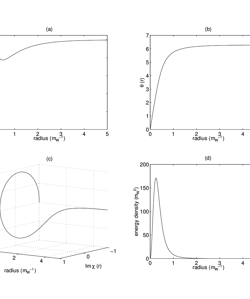
FIG. 1.: The soliton configuration for $\xi=12$. Panels a) and b) show $\rho$ and $\theta$ as functions of $r$ measured in units of the inverse $W$-mass. Note that $\theta$ changes by $2\pi$. Panel c) shows $\chi=-i\rho\exp(i\theta)$ vs. $r$. The projection of this curve onto the $\chi$-plane is shown in Figure 2. In panel d) we show the energy density vs. $r$. By energy density we mean $r^{2}$ times the $3$-dimensional energy density; the total energy of the configuration is the area under this curve.

and the energy density for the electroweak soliton with $\xi=12$. In Figure 2, we show how $\chi_{\rm sol}$ changes with $\xi$. For $\xi$ approaching $\xi^{*}$, the soliton configuration does not change qualitatively, and in particular $\rho$ remains well away from zero and $n$ remains 1. In the $\xi\rightarrow\infty$ limit, $\rho\rightarrow 1$, $a_{1}\rightarrow 0$ like $m/\sqrt{\xi}$, and the size of the soliton, i.e. the size of the region over which $\theta$ varies, shrinks like $1/(m\sqrt{\xi})$.

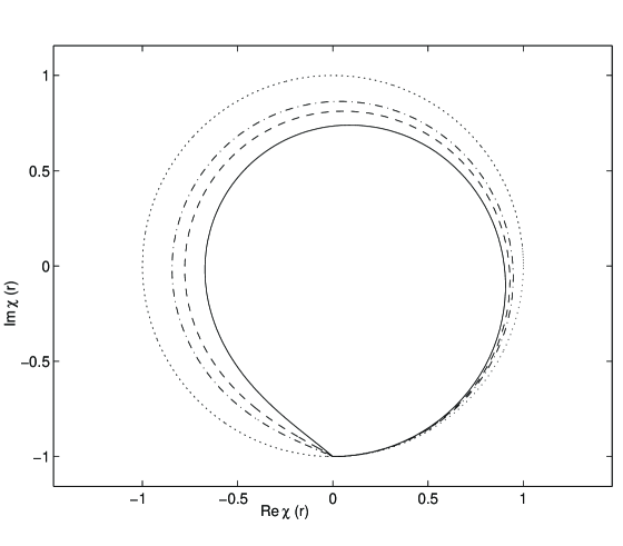
FIG. 2.: $\chi$ for the electroweak soliton for different values of $\xi$. All the curves begin at $\chi=-i$ at $r=0$, traverse a counter-clockwise loop which encircles $\chi=0$, and return to $\chi=-i$ as $r$ goes to infinity. The dotted, dot-dashed, dashed, and solid lines correspond to $\xi=\infty$, $15$, $12$, and $10.5$ respectively. Recall that there is no stable soliton for $\xi<\xi^{*}=10.35$. The range of $r$ over which the loops are traversed, i.e. the size of the soliton, is approximately $2/(m\xi^{1/2})$. At $\xi=\infty$, $|\chi|=1$ and the dotted curve is a circle. This reflects the fact that as $\xi$ approaches infinity the soliton configuration approaches the form (2.10).

We now consider initial conditions with a soliton and an incoming pulse which destroys the soliton. We have experimented with several ansätze for the pulse shape. Here we present one which we feel is fairly simple and which does destroy the soliton. Recall that for the soliton $\chi=-i$ at $r=0$ and wraps once around the origin as $r$ increases from $0$ to infinity. At $t=0$, the incident pulse we choose has $\chi_{\rm pulse}=\chi_{\rm vac}=-i$ for $r\leq r_{0}$ (where $r_{0}$ is large compared to the soliton) and has $\chi_{\rm pulse}\rightarrow\chi_{\rm vac}$ as $r\rightarrow\infty$. As $r$ increases from $r_{0}$, we choose $\chi_{\rm pulse}$ to loop in the complex plane in the opposite direction to that in which $\chi_{\rm sol}$ winds. $\chi_{\rm pulse}$ is a small enough excitation about $\chi_{\rm vac}$ that $|\chi_{\rm pulse}-\chi_{\rm vac}|<1$ and the pulse has $n=0$. Specifically, as the initial condition for $\chi$ we use

$$\chi=\left(\chi_{\rm sol}-\chi_{\rm vac}\right)+\chi_{\rm pulse}$$ (31)

where

$$\chi_{\rm pulse}=-i+\frac{ib}{2}\left[e^{2\pi ig(r)}-1\right]\ ,$$ (32)

with $b$ a constant whose absolute value is less than one and with the function $g(r)$ given by

$$g(r)=\cases{\exp\left[-(r-r_{0})^{2}/\sigma^{2}\right]~{};&$r>r_{0}$\cr 1~{};&$r\leq r_{0}$\cr}\ .$$ (33)

We choose initial conditions with $a_{1}=a_{1}^{\rm sol}$ and with $\dot{a}_{1}$ such that $a_{0}=0$. Now, we must specify $\dot{\chi}$. We wish to do this in such a way that the energy of the pulse propagates inward toward the soliton rather than outward toward large $r$. In a massive theory, it is impossible to achieve this exactly, and we use the following prescription which works well enough for our purposes. For $\chi=\chi_{\rm pulse}$ given by (32) and (33), $(\chi-\chi_{\rm vac})$ has a mean wave number squared of approximately $(\pi/\sigma)^{2}$ and a mean frequency $\omega\sim\sqrt{m^{2}+(\pi/\sigma)^{2}}$. So, we define a velocity

$$v=\frac{\pi/\sigma}{\sqrt{m^{2}+\left(\pi/\sigma\right)^{2}}}$$ (34)

and choose the initial condition

$$\dot{\chi}=v\,\frac{d\chi_{\rm pulse}}{dr}\ .$$ (35)

Thus, in this ansatz the initial conditions are parametrized by the amplitude $b$, the pulse width $\sigma$ and the initial radius $r_{0}$.

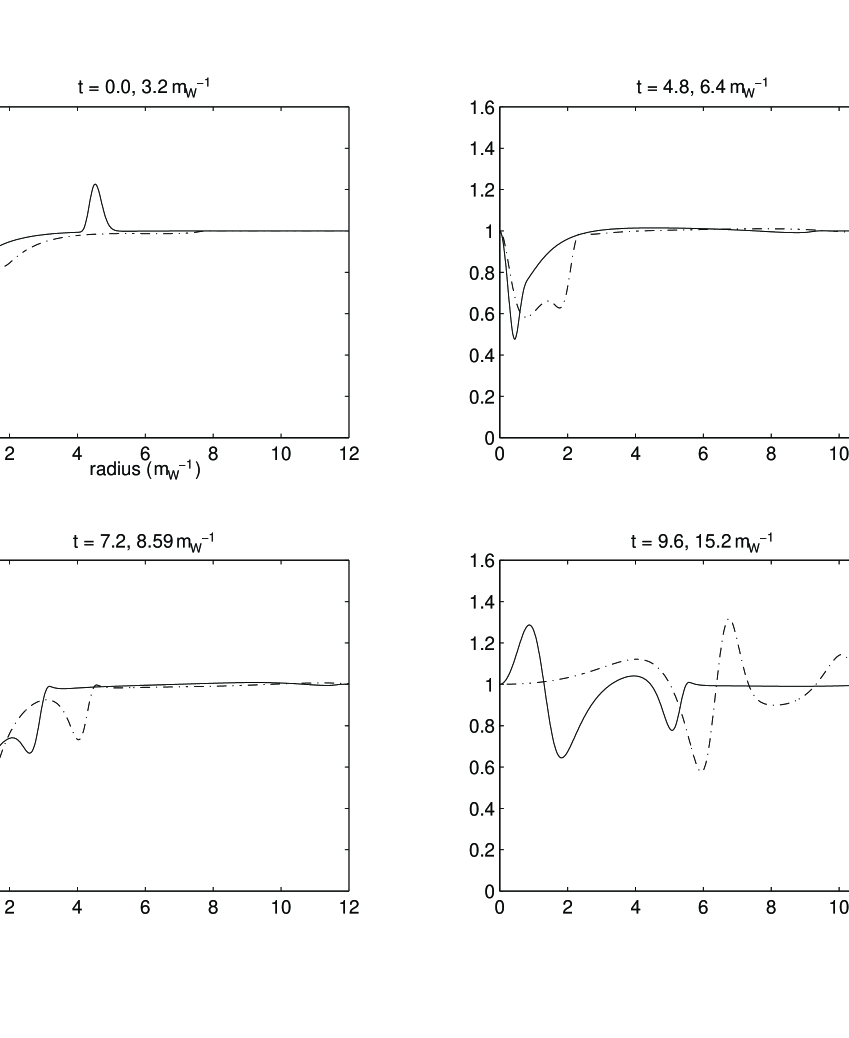
FIG. 3.: This figure, which continues on the following pages, shows the destruction of the $\xi=12$ soliton by the pulse specified in the text. The simulations were done on a lattice which extended to $r=16/m$, but only $0\leq r\leq 12/m$ is displayed. On this page, we show snapshots of $\rho(r)$ at eight different times. Each panel displays $\rho(r)$ at two times; the solid curve shows $\rho(r)$ at the earlier time, and the dot-dashed curve shows $\rho(r)$ at the later time. For example, in the first panel the solid curve at $t=0.0/m$ shows the incident pulse superimposed on the soliton of Figure 1. The dot-dashed curve shows $\rho$ at $t=3.2/m$ when the pulse has moved inward toward $r=0$. By $t=4.8/m$, the solid curve in the second panel, it is clear that the soliton has been disturbed. At $t=7.2/m$, there is an outgoing pulse at $r\sim 3/m$ and the soliton has not returned to its initial shape. At $t=8.59/m$, $\rho=0$ at $r=0.94/m$. At $t=15.2/m$, the final time shown, there is an outgoing pulse at $r\sim 11/m$ followed by the outgoing remnants of the soliton at $r\sim 6/m$.

FIG. 3.: On this page, we show snapshots of $\theta(r)$ corresponding to the preceding snapshots of $\rho(r)$. We show two times per panel, and the solid curve is the earlier of the two. At all times before $t=8.59/m$, $\theta$ increases from $\theta=0$ at $r=0$ to $\theta=2\pi$ at large $r$. At $t=8.59/m$, note the large slope in $\theta$ at $r=0.94/m$ which is where $\rho$ vanishes. At later times, $\theta$ is no longer wound.

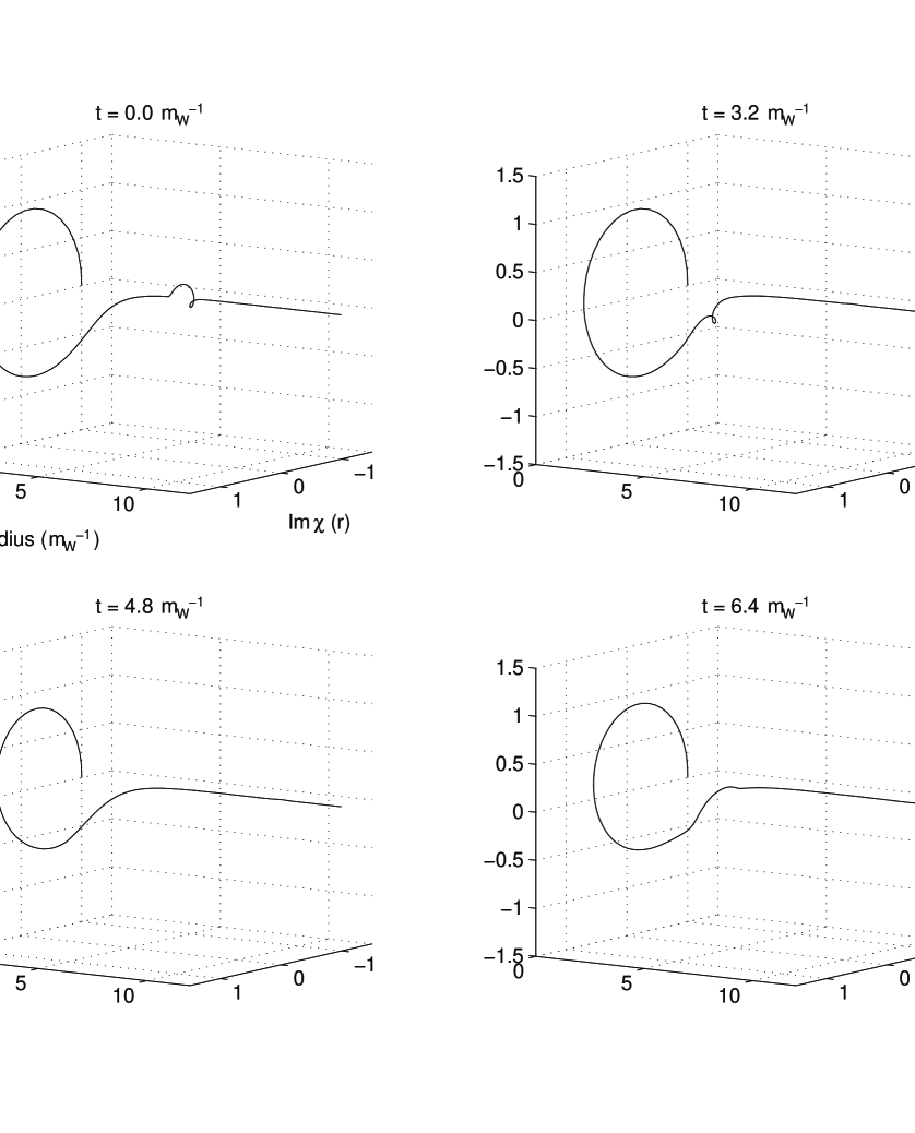
FIG. 3.: On this page and the next, we combine $\rho$ and $\theta$ from the previous pages into three-dimensional plots of $\chi=-i\rho\exp(i\theta)$ as a function of $r$ at eight times. Initially, we see the pulse incident upon the soliton. Between $t=6.4/m$ and $t=9.6/m$, we see the soliton shed an outgoing pulse, and then shrink from a loop which encircles $\chi=0$ to an excitation about the vacuum $\chi=-i$ which does not. At $t=15.2/m$, $\chi$ is close to the vacuum for small $r$, and at larger $r$ we see the outgoing pulse and the outgoing remnants of the soliton.

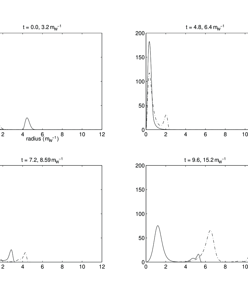
FIG. 3.: Finally, we show snapshots of the energy density at the same times as before. There are two times per panel, the solid line at the earlier time and the dot-dashed line at the later time. As in Figure 1, by energy density we mean $r^{2}$ times the $3$-dimensional energy density. At $t=0$, we see that the incident pulse has much less energy than the soliton, but nevertheless it destroys the soliton. The destruction of the soliton is seen most clearly by looking at $t=15.2/m$. At this time, there is no energy density visible for $r$ less than about $3/m$, which is where the soliton was at $t=0$. The soliton is no more. There is an outgoing pulse at $r\sim 11/m$ which has an energy comparable to but slightly lower than that of the incident pulse. This is followed at $r\sim 6/m$ by an outgoing shell with energy comparable to that of the soliton.

Figure 3 shows the result of hitting the soliton at $\xi=12$ with a pulse chosen using the above ansatz with $b=0.23$, $\sigma=\pi/5m$, and $r_{0}=4/m$. We plot $\rho$, $\theta$, $\chi$ and the energy density as functions of $r$ for a number of different times. First, note that the pulse does move inward toward the soliton. The soliton energy is $72.67\,m$, the sphaleron energy is $73.9\,m$, and the total energy of the solution is $85.85\,m$. Thus, neglecting the small amount of energy initially in the pulse which goes outward, the soliton is hit with a pulse with energy $E_{\rm pulse}=13.18\,m$ which is larger than $\Delta E=M_{\rm sph}-M_{\rm sol}=1.2\,m$. We see that at time $t=7.2/m$ there is an outgoing pulse with somewhat less energy than $E_{\rm pulse}$, and the soliton has been somewhat distorted, as it begins to fall apart. At time $t=8.59/m$, $\rho$ is very close to zero at $r=0.94/m$. At late times, we see from the plot of $\theta$ that the winding $n$ is zero, and we see from the plot of the energy that there is in fact no soliton present. We estimate $N$, the number of $W$-bosons in the incident pulse which destroyed the soliton, as

$$g^{2}N\sim\frac{E_{\rm pulse}}{\omega}\sim\frac{E_{\rm pulse}}{\sqrt{m^{2}+(\pi/\sigma)^{2}}}\sim 2.5\ .$$ (36)

We now sketch how the results of Figure 3 change as we vary $b$ and $\sigma$. First, upon increasing $b$ from $0.23$ (and thus increasing $E_{\rm pulse}$ and $g^{2}N$) the time delay between the emergence of an outgoing pulse and the collapse of the soliton decreases – the soliton is destroyed more promptly. Upon decreasing $b$, the time delay increases — less energy is delivered to the soliton and the soliton takes longer to fall apart. Decreasing $b$ further, we find a threshold somewhere between $b=0.21$ and $b=0.22$ below which the soliton survives. Below this threshold, after the emergence of an outgoing pulse, the soliton radiates any remaining excess energy outward and settles back to its undisturbed state. For several values of $\sigma$ ranging from half to twice that in Figure 3, the threshold $b$ is about the same.

We have worked at values of $\xi$ ranging from 10.5 to 100. For a given $\sigma$ the threshold amplitude is lower for values of $\xi$ closer to $\xi^{*}$. For $\xi=11$, for example, we have found soliton destroying pulses with $g^{2}N\sim 1$. As $\xi$ becomes very large the soliton size ($\sim 1/(m\sqrt{\xi})$) becomes much smaller than the sphaleron size ($\sim 1/m$) and the barrier height $\Delta E$ grows like $M_{\rm sol}\sqrt{\xi}$. At large $\xi$, therefore, the energy of soliton destroying pulses must become large compared to $M_{\rm sol}$ and large compared to the inverse sphaleron size. It is nevertheless a logical possibility that such pulses could be found with high frequencies and small values of $g^{2}N$. For $\xi=50$ and above, however, we have only found soliton destroying pulses which have large $g^{2}N$. This suggests that because at large $\xi$ the soliton is no longer similar to the sphaleron, we lose the advantage that we have in this model, relative to the standard model, in finding sphaleron crossing solutions with $g^{2}N$ small.

We have chosen to present results for $\xi=12$ (rather than choosing $\xi$ closer to $\xi^{*}$ where the threshold amplitude and threshold $g^{2}N$ are lower) because at $\xi=12$ the tunnelling lifetime of the soliton is much longer than any time scale in Figure 3. As we discuss in Section V, Rubakov, Stern and Tinyakov[13] write the tunnelling lifetime as as $\tau\sim(1/m)\exp(2B)$ and calculate that $g^{2}B=4\pm 1$ for $\xi=12$. Thus, for $g=0.65$ and $\xi=12$, $\tau\sim 10^{8}/m$.

We have tried a number of incident pulse shapes that do not fall into the ansatz we have described in detail, and have found qualitatively similar results. For all the cases which we have considered with $\xi$ within a factor of two of $\xi^{*}$, we have observed that as we vary the amplitude of a pulse whose size is comparable to that of the soliton, for amplitudes above some threshold the soliton is destroyed. For a given pulse shape, the threshold energy and threshold $g^{2}N$ decrease as $\xi$ decreases toward $\xi^{*}$. Among the few pulse shapes which we tried, the threshold energy was lowest for the ansatz of (32), but we have certainly not found the lowest energy or lowest particle number pulses which destroy the soliton. Indeed, a soliton destroying pulse with energy just above $\Delta E$ could be obtained by starting with a slightly perturbed sphaleron, watching it decay to the soliton, and then time reversing. We will see in Section IV that for $\xi$ near $\xi^{*}$ a “pulse” so obtained would be a very long train of small amplitude waves, rather than a simple pulse of the kind we have used to destroy solitons in our numerical experiments.

The lesson of this section is that in the model we are treating, it is straightforward to find soliton destroying, sphaleron crossing, fermion number violating classical solutions. Particular pulse profiles are not required — pulses of any shape we have tried (with sizes comparable to the soliton size) destroy the soliton if their energy is above some shape-dependent threshold.

III Quantum Implications of Classical Solutions which Destroy Solitons

In a theory like the ungauged Skyrme model with a static classical solution which is absolutely stable, that is, separated by an infinite energy barrier from the classical vacuum configuration, the Hilbert space of the quantized theory separates into sectors with a fixed number of solitons, and states in different sectors have zero overlap[16]. The one soliton sector, for example, is a Fock space of states with one soliton and any number of mesons. The mesons (pions in the Skyrme model) are the quantized fluctuations about the soliton configuration, and the states in the one soliton sector are scattering states of mesons in the presence of a soliton. No process, not even one involving large numbers of mesons, connects states in the one soliton sector with states in the vacuum sector.

In our theory, the electroweak soliton is not absolutely stable. It is separated by a barrier of finite height from the vacuum. The Hilbert space has sectors with a fixed number of solitons and any number of $W$-bosons. However, we now argue that the existence of the classical solutions described in the previous section, in which incident pulses destroy a soliton, demonstrates that there are states in the zero and one soliton sectors with nonzero overlap.

Consider a classical solution obtained by taking a solution in which a soliton is destroyed and the time reverse of a different such solution and combining them as we now describe. At very early times, there are two incoming pulses widely separated in time. The inner pulse, of total energy $E_{1}$, is the time reverse of a solution of the kind found in Section II. It forms a soliton, an outgoing pulse of energy $E_{1}-M_{\rm sol}$ is radiated, and the soliton of mass $M_{\rm sol}$ is left sitting at the origin. Then the outgoing pulse passes the second incoming pulse at a radius large enough that the amplitudes of both pulses are small, and no interaction occurs. Subsequently, the second pulse of total energy $E_{2}$ arrives at the soliton and destroys it, yielding a second outgoing pulse of energy $E_{2}+M_{\rm sol}$. At very late times there is no soliton present, and there are two outgoing pulses. This entire solution falls into the class of classical solutions discussed in Appendix B, in that at very early and very late times the fields are small amplitude excitations about the vacuum. By the arguments of Appendix B, the existence of this solution implies that we can construct normalized coherent states

$$|f^{1}_{\rm in},f^{2}_{\rm in}\rangle$$ (37)

and

$$|f^{1}_{\rm out},f^{2}_{\rm out}\rangle$$ (38)

such that

$$\langle f^{1}_{\rm out},f^{2}_{\rm out}|f^{1}_{\rm in},f^{2}_{\rm in}\rangle=\exp\left\{\frac{i\theta}{g^{2}}+{\cal O}(g^{0})\right\}$$ (39)

as $g\rightarrow 0$, with $\theta$ a real phase. The energy and particle number in the in and out states are ${\cal O}(1/g^{2})$. Equation (B30) expresses $\theta$ as an integral of the classical fields over space-time. When the time separation $T$ between the pulses $1$ and $2$ is large compared to the times necessary for the formation and destruction of the soliton, this integral can be written as the sum of three terms,

$$\frac{\theta}{g^{2}}=\frac{\theta_{1}}{g^{2}}+\frac{\theta_{2}}{g^{2}}+M_{\rm sol}T$$ (40)

where $\theta_{1}$ depends only on $f^{1}_{\rm out}$ and the formation solution, $\theta_{2}$ only on $f^{2}_{\rm in}$ and the destruction solution, and $M_{\rm sol}$ is the classical energy of the soliton which is of order $1/g^{2}$.

With this information concerning asymptotic states, the only possible interpretation is that there are coherent states of $W$-bosons in the one soliton sector $|{\rm sol},f^{1}_{\rm out}\rangle$ and $|{\rm sol},f^{2}_{\rm in}\rangle$, and that

$$\langle{\rm sol},f^{1}_{\rm out}|f^{1}_{\rm in}\rangle=\exp\left\{\frac{i\theta_{1}}{g^{2}}+{\cal O}(g^{0})\right\}$$ (41)

$$\langle f^{2}_{\rm out}|{\rm sol},f^{2}_{\rm in}\rangle=\exp\left\{\frac{i\theta_{2}}{g^{2}}+{\cal O}(g^{0})\right\}\ .$$ (42)

Thus there are processes connecting the one-soliton sector to the vacuum sector which are not exponentially suppressed as $g\rightarrow 0$, though they do involve ${\cal O}(1/g^{2})$ $W$-bosons.

In the remainder of this paper our goal is to study quantum processes in which a single $W$-boson incident upon the soliton kicks it over the barrier causing it to decay. In Section V, we will do a controlled calculation of this process in a limit in which $\xi$ goes to $\xi^{*}$ as $g$ goes to zero. In order to do this calculation, however, we first need a better understanding of classical dynamics of the theory with $\xi$ near $\xi^{*}$, and to this we now turn.

IV Classical Dynamics for $\xi$$\xi$$\xi$ near ${\kern-0.24994pt\hbox{$\xi$}\kern-4.37502pt\kern 0.50003pt\hbox{$\xi$}\kern-4.37502pt\kern-0.24994pt\raise 0.43304pt\hbox{$\xi$}}^{\bf*}$

In order to discuss the special features of the dynamics of our system for $\xi$ near $\xi^{*}$, and because we will need it to discuss the quantum version of this theory, we introduce the Hamiltonian which arises from (11):

$$H=\int{\rm d}^{3}{\bf x}\left\{{g^{2}}{\rm Tr}\,\Pi^{i}\Pi^{i}+\frac{1}{g^{2}}\left[\frac{1}{2}{\rm Tr}\,F^{ij}F^{ij}-m^{2}{\rm Tr}\,A_{\mu}A^{\mu}-\frac{1}{8\xi}{\rm Tr}\left[A_{\mu}\,,\,A_{\nu}\right]^{2}\right]-2{\rm Tr}\left[A_{0}D_{i}\Pi^{i}\right]\right\}$$ (43)

where

$$\Pi^{i} = \frac{1}{g^{2}}\,F^{i0}$$ (44)

$$D_{i}\Pi^{i} = \partial_{i}\Pi^{i}-i\left[A_{i}\,,\,\Pi^{i}\right]\ .$$ (45)

Now $A^{0}$ has no conjugate momentum and the $A^{0}$ equation is

$$m^{2}A^{0}+\frac{1}{4\xi}\left[\,\left[A^{i}\,,\,A^{0}\right],A_{i}\right]+g^{2}D_{i}\Pi^{i}=0\ .$$ (46)

This linear equation for $A^{0}$ can be solved giving $A^{0}$ in terms of $A^{i}$ and $\Pi^{i}$ but we do not need to do this explictly. The Hamiltonian for our system is given by (43) with $A^{0}$ determined by (46) and has the general form

$$H=\frac{g^{2}}{2}\,\Pi\,M^{-1}(A)\,\Pi+\frac{1}{g^{2}}\,V[A]\ ,$$ (47)

where the sum over the coordinate ${\bf x}$, the spatial index $i$ and the group index are all implicit. The matrix $M^{-1}(A)$ involves derivatives with respect to ${\bf x}$, depends on the configuration $A$, and we assume that $M^{-1}(A)$ is positive. Note that static solutions to the equations of motion, that is those with $\dot{\Pi}=\dot{A}=0$, occur where $\delta V/\delta A=0$ and have $\Pi=0$. The classical equation of motion for $A$ which arises from (47) is independent of $g$. Thus for the discussion of classical dynamics which we are having in this chapter, we can set $g=1$. We will restore the $g$ dependence in the next chapter.

The potential energy functional $V[A]$ has its overall scale set by $m$ but the topography of fixed energy contours is set by $\xi$. Ambjorn and Rubakov [10] showed that for $\xi>\xi^{*}=10.35$ there is a local minimum, the soliton, whereas for $\xi<\xi^{*}$ this minimum is absent. For $\xi>\xi^{*}$ there is also a sphaleron, that is a saddle point configuration whose energy is greater than that of the soliton. As $\xi$ approaches $\xi^{*}$ from above, the sphaleron and soliton merge.

We are particularly interested in configurations which, at least initially, are small perturbations around the soliton. To work with these configurations we find it convenient to make a canonical transformation which has the effect of setting $M^{-1}(A_{\rm sol})=1$ and $\frac{{\rm d}M^{-1}}{{\rm d}A}\bigg{|}_{A_{\rm sol}}=0$. To see that this is possible let $f_{\alpha}$ be some complete set of orthonormal, spatial vector, matrix-valued functions of ${\bf x}$, indexed by $\alpha$, which can be used to expand $\Pi$ and $A$. Let the coefficients of the expansion of $A$ relative to the soliton be $q^{\alpha}$ and the coefficients of the expansion of $\Pi$ be $p_{\alpha}$, that is

$$A({\bf x},t)-A^{\rm sol}({\bf x}) = \sum_{\alpha}q^{\alpha}(t)f_{\alpha}({\bf x})$$ (48)

$$\Pi({\bf x},t) = \sum_{\alpha}p_{\alpha}(t)f_{\alpha}({\bf x})\ .$$ (49)

(Note that the transformation from $A({\bf x},t)$, $\Pi({\bf x},t)$ to $q^{\alpha}(t)$, $p_{\alpha}(t)$ is canonical.) Upon making this transformation, (47) has the form

$$H=\frac{1}{2}\,g^{\alpha\beta}(q)p_{\alpha}p_{\beta}+V(q)\ .$$ (50)

A canonical transformation of the form

$$q^{\prime\alpha}=q^{\prime\alpha}(q)~{}~{}~{}{\rm and}~{}~{}~{}p^{\prime}_{\alpha}=\frac{\partial q^{\beta}}{\partial q^{\prime\alpha}}p_{\beta}$$ (51)

can be viewed as a general coordinate transformation with $p_{\alpha}$ transforming as a covariant vector. It is always possible to choose coordinates such that

$$g^{\prime\alpha\beta}=\frac{\partial q^{\prime\alpha}}{\partial q^{\delta}}\,\frac{\partial q^{\prime\beta}}{\partial q^{\epsilon}}\,g^{\delta\epsilon}$$ (52)

is equal to $\delta^{\alpha\beta}$ with $\partial g^{\prime\alpha\beta}/\partial q^{\prime\epsilon}=0$ at any given point. In fact this can be accomplished at $q^{\alpha}=0$ (the soliton) with a transformation of the form $q^{\prime\alpha}=C^{\alpha}_{\beta}q^{\beta}+C^{\alpha}_{\beta\delta}q^{\beta}q^{\delta}$. This means that the Hamiltonian (50) can be written as

$$H=\frac{1}{2}\,p_{\alpha}\left[\delta^{\alpha\beta}+{\cal O}(q^{2})\right]p_{\beta}+V(q)\ ,$$ (53)

where we have made the required canonical transformation and dropped the primes. Note that $V(q=0)=M_{\rm sol}$ and $(\partial V/\partial q^{\alpha})|_{q=0}=0$.

For $\xi>\xi^{*}$ consider small oscillations about the soliton. The frequencies squared are given by the eigenvalues of the fluctuation matrix $\partial^{2}V/\partial q^{\alpha}\partial q^{\beta}$ at $q=0$. The soliton is a localized object so fluctuations far from the soliton propagate freely. Therefore the fluctuation matrix at the soliton has a continuous spectrum above $m^{2}$. A given soliton configuration and a translation or rotation of that configuration have the same energy and both solve $\partial V/\partial q^{\alpha}=0$. This implies that at $q=0$ there are six zero eigenvalues of $\partial^{2}V/\partial q^{\alpha}\partial q^{\beta}$. The associated modes which correspond to translating and rotating the soliton are not of interest to us and will be systematically ignored.

For $\xi$ close to $\xi^{*}$ we now argue that there is one normalizable mode whose frequency $\omega_{0}$ goes to zero as $\xi$ goes to $\xi^{*}$. To see this we write

$$\frac{\partial V}{\partial q^{\alpha}}\Bigg{|}_{q_{\rm sph}}=\frac{\partial V}{\partial q^{\alpha}}\Bigg{|}_{q=0}+\frac{\partial^{2}V}{\partial q^{\alpha}\partial q^{\beta}}\Bigg{|}_{q=0}q^{\beta}_{\rm sph}+\frac{1}{2}\,\frac{\partial^{3}V}{\partial q^{\alpha}\partial q^{\beta}\partial q^{\epsilon}}\Bigg{|}_{q=0}q^{\beta}_{\rm sph}q^{\epsilon}_{\rm sph}+\ldots\ .$$ (54)

At the soliton ($q=0$) and at the sphaleron the first derivatives are zero. As $\xi$ approaches $\xi^{*}$ the sphaleron and soliton merge so $q^{\alpha}_{\rm sph}$ goes to zero. It is useful to introduce the normalized function $\bar{q}_{\rm sph}$

$$\bar{q}^{\alpha}_{\rm sph}=\frac{q^{\alpha}_{\rm sph}}{Q}$$ (56)

where

$$Q^{2}=\sum_{\alpha}q^{\alpha}_{\rm sph}q^{\alpha}_{\rm sph}\ .$$ (57)

As $\xi$ goes to $\xi^{*}$, $Q$ goes to zero but $\bar{q}_{\rm sph}$ does not. From (54) we then have

$$\frac{\partial^{2}V}{\partial q^{\alpha}\partial q^{\beta}}\Bigg{|}_{q=0}\bar{q}^{\alpha}_{\rm sph}\bar{q}^{\beta}_{\rm sph}=-\frac{1}{2}Q\frac{\partial^{3}V}{\partial q^{\alpha}\partial q^{\beta}\partial q^{\epsilon}}\Bigg{|}_{q=0}\bar{q}^{\alpha}_{\rm sph}\bar{q}^{\beta}_{\rm sph}\bar{q}^{\epsilon}_{\rm sph}+{\cal O}(Q^{2})\ .$$ (58)

For $\xi>\xi^{*}$ the fluctuation matrix $\partial^{2}V/\partial q^{\alpha}\partial q^{\beta}$ at the soliton has only positive eigenvalues (except for the translation and rotation zero modes which play no role in this discussion). Equation (58) tells us that at $\xi=\xi^{*}$ where $Q=0$, the fluctuation matrix has a zero eigenvalue with eigenvector $\bar{q}_{\rm sph}$ whereas for $\xi$ close to $\xi^{*}$ there is a small eigenvalue, $\omega_{0}^{2}$, whose associated eigenvector is close to $\bar{q}_{\rm sph}$. Note that $\bar{q}_{\rm sph}$ points from the soliton to the sphaleron. Thus the low frequency mode, which we call the $\lambda$-mode, is an oscillation about the soliton close to the direction of the sphaleron.

For $\xi>\xi^{*}$, at the sphaleron there is one negative mode, that is one negative eigenvalue of the appropriately defined fluctuation matrix. As $\xi$ comes down to $\xi^{*}$ the sphaleron and soliton become the same configuration so this negative eigenvalue must come up to zero in order for the spectra of the fluctuation matrices of the soliton and sphaleron to agree at $\xi=\xi^{*}$. Therefore for $\xi$ close to $\xi^{*}$ the unstable direction off the sphaleron has a small negative curvature. There are two directions down from the sphaleron. One heads toward the soliton and the other heads (ultimately) to the classical vacuum at $A=0$. We see that for $\xi$ near $\xi^{*}$ the soliton can be destroyed by imparting enough energy to the $\lambda$-mode since it is this mode which is pointed towards the sphaleron and beyond.

We wish to describe the interaction of the $\lambda$-mode with the other degrees of freedom. We use the Hamiltonian written in the form (53). At this point it is convenient to make an orthogonal transformation on the $\{q^{\alpha}\}$ so that the transformed set are the eigenvectors of the soliton fluctuation matrix $\partial^{2}V/\partial q^{\alpha}\partial q^{\beta}|_{q=0}$. We will label these vectors as $q_{\omega}$ where $\omega^{2}$ is the eigenvalue of the fluctuation matrix. The eigenfunctions include:

• The continuum states $q_{\omega}$ with eigenvalues $\omega^{2}>m^{2}$. (Note that for each $\omega^{2}$, in general, there is more than one eigenvector. The extra labels on $q_{\omega}$ are suppressed in our compact notation.)

• The normalizable state $q_{\omega_{0}}\equiv\lambda$ with eigenvalue $\omega_{0}^{2}$ which goes to zero as $\xi$ goes to $\xi^{*}$.

• The zero eigenvalue states associated with translation and rotation.

• Other normalizable states which might exist but whose frequencies do not have any reason to approach zero as $\xi$ goes to $\xi^{*}$.

Up to cubic order the Hamiltonian (53) is

$$H=M_{\rm sol} + \frac{1}{2}p^{2}+\frac{1}{2}\omega_{0}^{2}\lambda^{2}+\frac{b}{3}\lambda^{3}$$ (59)

$$+ \frac{1}{2}\int_{m}{\rm d}\omega\,p_{\omega}^{2}+\frac{1}{2}\int_{m}{\rm d}\omega\,\omega^{2}\,q_{\omega}^{2}+\int_{m}{\rm d}\omega{\rm d}\omega^{\prime}{\rm d}\omega^{\prime\prime}\,c(\omega,\omega^{\prime},\omega^{\prime\prime})\,q_{\omega}q_{\omega^{\prime}}q_{\omega^{\prime\prime}}$$ (60)

$$+ \lambda^{2}\int_{m}{\rm d}\omega\,d(\omega)q_{\omega}+\lambda\int_{m}{\rm d}\omega{\rm d}\omega^{\prime}\,e(\omega,\omega^{\prime})q_{\omega}q_{\omega^{\prime}}+\ldots$$ (61)

where in the ellipses we now include all terms with modes of type iii) and iv) as well as higher order interactions of the $\lambda$-mode and the continuum modes. $p$ is the momentum conjugate to $\lambda$ and $p_{\omega}$ is the momentum conjugate to $q_{\omega}$. The number $b$ and the functions $c$, $d$ and $e$ are determined by the soliton configuration. For example $d(\omega)$ is presumably peaked at values of $\omega$ which correspond to wavelengths of order the size of the soliton. As $\xi$ goes to $\xi^{*}$ we know that $\omega_{0}$ goes to zero but we expect no dramatic behavior of $b$, $c$, $d$ or $e$ in this limit.

Consider the $\lambda$-mode potential

$$V(\lambda)=\frac{1}{2}\omega_{0}^{2}\lambda^{2}+\frac{b}{3}\lambda^{3}+\ldots\ .$$ (62)

There is a local minimum at $\lambda=0$ which is the soliton and a local maximum at $\lambda=-\omega_{0}^{2}/b$, which is approximately the sphaleron, where the second derivative is $-\omega_{0}^{2}$. We work with $\xi$ sufficiently close to $\xi^{*}$ that $\omega_{0}$ is small. This means that $\lambda$ at the sphaleron is small and if we only study dynamics up to and just beyond the sphaleron we are justified in neglecting the quartic and higher terms in $\lambda$. We also see that as $\xi$ goes to $\xi^{*}$ so that $\omega_{0}$ goes to zero, the soliton and sphaleron come together and at $\xi=\xi^{*}$ the $\lambda$ potential has an inflection point at $\lambda=0$ and the soliton is no longer classically stable.

In order to discover the relationship between $\omega_{0}$ and $(\xi-\xi^{*})$ as $\xi$ approaches $\xi^{*}$, it is necessary to study the behavior of the $\lambda$-mode potential as $\xi$ approaches $\xi^{*}$. In (62) for every value of $\xi$, we have shifted $\lambda$ so that the minimum of the potential is at $\lambda=0$. This $\xi$ dependent change of variables obscures the behavior of the coefficients of the potential before the shift. Calling the unshifted variable $\bar{\lambda}$, then if we expand the potential in terms of $\epsilon\equiv\xi-\xi^{*}$ about $\epsilon=0$ where there is an inflection point, we have

$$V(\bar{\lambda},\epsilon)={\cal O}(\epsilon)\bar{\lambda}+{\cal O}(\epsilon)\bar{\lambda}^{2}+\Big{(}\bar{b}+{\cal O}(\epsilon)\Big{)}\bar{\lambda}^{3}+\ldots\ ,$$ (63)

where $\bar{b}$ is a constant. We know that the coefficients of $\bar{\lambda}$ and $\bar{\lambda}^{2}$ are zero at $\epsilon=0$, and we assume that these coefficients can be expanded about $\epsilon=0$ and we know of no reason for the order $\epsilon$ terms to vanish. For $\epsilon>0$ the minimum of the potential is at $\bar{\lambda}\sim\epsilon^{1/2}$, ($\lambda$ is shifted relative to $\bar{\lambda}$ by this amount), and at the minimum of the potential $\partial^{2}V/\partial\bar{\lambda}^{2}\sim\epsilon^{1/2}$, that is

$$\omega_{0}^{2}\sim(\xi-\xi^{*})^{1/2}\ .$$ (64)

A small amplitude oscillation of the $\lambda$ mode will decay because of its coupling to the continuum modes which can carry energy away from the soliton. However for $\omega_{0}<m$ this decay is very slow in the sense that the characteristic time for the decay is much greater than $1/\omega_{0}$. To understand this consider $\lambda(t)$ as a source for radiation in the continuum via the coupling $\lambda^{2}\int_{m}{\rm d}\omega d(\omega)q_{\omega}$ in the Hamiltonian (61). Suppose that $\lambda(t)$ is a purely sinusoidal oscillation with frequency $\omega_{0}$ and with an amplitude which is small. Radiation with frequency $\omega_{0}$ is not possible because the continuum frequencies begin at $\omega=m$. However, $\lambda^{2}$ has frequency $2\omega_{0}$ and therefore if $\omega_{0}>m/2$ the coupling will excite propagating modes with $\omega=2\omega_{0}$ and the $\lambda$ oscillation will radiate at twice its fundamental frequency. Because the coupling is of order $\lambda^{2}$, the rate of energy loss will be small. If $\omega_{0}<m/2$ then radiation at $\omega=2\omega_{0}$ is also not possible. However, if $m/3<\omega_{0}<m/2$ the $\lambda^{3}q_{\omega}$ coupling (which we have not written in (61) because it is fourth order) allows the $\lambda$ oscillation to radiate at three times its fundamental frequency. There is another source of radiation with $\omega=3\omega_{0}$. The potential for the $\lambda$-mode is not exactly quadratic so the $\lambda$ oscillation, although periodic, is not exactly sinusoidal. If the period of the oscillation is $2\pi/\omega_{0}$, $\lambda$ will be a sum of terms of the form $\sin\omega_{0}t$, $\sin 2\omega_{0}t$, $\sin 3\omega_{0}t$,… with diminishing coefficients. This means that $\lambda^{2}$ will also be a sum of terms of this form. Those terms in $\lambda^{2}$ with frequencies greater than $m$ will excite radiation via the $\lambda^{2}q_{\omega}$ coupling. As $\omega_{0}$ is reduced from $m$ toward zero, the radiation is produced only by higher order couplings and by higher harmonics, and therefore the amplitude is reduced and the decay takes longer.

We have numerical evidence for this behavior within the spherical ansatz. To watch an oscillating soliton radiate for a long time, we implement energy absorbing boundary conditions at the large $r$ boundary of the simulation lattice, as described in Appendix A. We wish to excite the $\lambda$-mode and watch it oscillate. It is convenient to choose initial conditions by starting with some $n=1$ configuration and evolving it using the equations of motion with damping terms added as described in Section II. Instead of running for long enough that the configuration is damped down to the soliton, we stop somewhat earlier. This yields a configuration which is the soliton plus a small perturbation. Because the damping terms damp modes with higher frequencies more quickly than those with lower frequencies, the perturbation that remains is mostly in the lowest few modes. We use the configuration just described as the initial condition for the equations of motion with no damping terms.

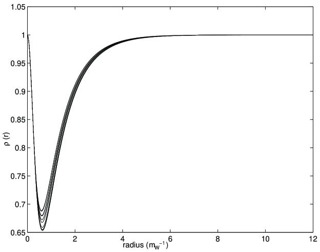
FIG. 4.: As described in the text, we have perturbed the $\xi=10.4$ soliton and let it evolve for a long time. Here, we show $\rho(r)$ for a series of different times: $t=0$, $144$, $288$, $\ldots$ $1440$ $m^{-1}$. This shows the envelope of the oscillation of $\rho$. In Figure 5, we show $\rho$ at $r=0.608/m$ and $r=10/m$ as a function of time.

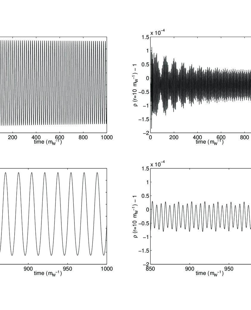
FIG. 5.: In the left panels, we show $\rho$ at $r=0.608/m$ as a function of time. It oscillates with period $16.69/m$, and the amplitude of the oscillation is decreasing very slowly. In the right panels, we show $\rho$ at $r=10/m$, to display the outgoing travelling waves shed by the oscillating soliton. These waves have three times the frequency of the fundamental oscillation seen at $r=0.608/m$. Note that the amplitude of the outgoing waves is so small that they are invisible in the plots of $\rho(r)$ on the preceding page. We conclude that for $\xi=10.4$ the soliton has an almost stable mode of oscillation with frequency $\omega_{0}=0.374\,m$ — the $\lambda$-mode — which slowly radiates waves with frequency $3\,\omega_{0}$.

The resulting evolution is shown in Figures 4 and 5 for $\xi=10.4$. The functions $\rho$, $\theta$, and $a_{1}$ (we show $\rho$ only) all oscillate about the values they take at the soliton and the period of oscillation is $16.69\,m^{-1}$. We identify this with the $\lambda$-mode and so obtain $\omega_{0}=0.3764\,m$. Furthermore we see that away from the soliton there is a small amplitude train of outgoing radiation. After a brief initial period during which any perturbations not in the $\lambda$-mode radiate away, the outgoing radiation settles down to a frequency $1.129\,m$, three times the fundamental frequency. (At $r=10\,m^{-1}$, we see in Figure 5 that the frequency $3\omega_{0}$ oscillation of $\rho$ has a small modulation with frequency $\omega_{0}$. This is the tail of the $\lambda$-mode oscillation and is not seen at larger values of $r$.) The radiation causes the amplitude of the $\lambda$-mode to decrease very slowly — by about $4\%$ over $80$ oscillations. We have done similar simulations at $\xi=11$ and $\xi=12$ also, where we find $\omega_{0}=0.80\,m$ and $\omega_{0}=0.98\,m$ respectively. In these simulations, the oscillating soliton emits radiation with $\omega=2\omega_{0}$, and the amplitude of the radiation and the rate of decay of the fundamental oscillation are larger than in Figure 5. The values of $\omega_{0}$ for $\xi=10.4$, $11$, and $12$ which we have found numerically are in good agreement with the relationship (64). This numerical evidence suggests that we are justified in using the Hamiltonian (61) to describe the long-lived normalizable $\lambda$-mode with $\omega_{0}<m$ and its coupling to the continuum. In the next chapter we will quantize this Hamiltonian and use it to describe the excitation of the $\lambda$-mode by single $W$-boson quanta.

Finally we note that in principle it is possible to destroy a soliton with a minimum energy pulse, i.e. one whose energy is just above $\Delta E$, and for $\xi$ close to $\xi^{*}$ this energy is small. To find the form of this pulse we could time reverse a solution which starts at the sphaleron and is given a gentle push towards the soliton. For $\xi$ close to $\xi^{*}$ so that the $\lambda$-mode has a small frequency, the configuration takes a very long time to settle down to the soliton and in the process emits a very long train of low amplitude outgoing waves. Although the time-reversed solution consisting of a very long train of incoming low amplitude waves being absorbed by the soliton would eventually go over the sphaleron barrier and result in soliton decay, it would be rather difficult to set up initial conditions which produce this complicated, finely tuned, incoming configuration. Thus, the minimum energy soliton destroying pulses are not easy to build although we saw in Section II that with some extra energy, for $\xi$ near $\xi^{*}$, the soliton is easily killed.

V Quantum Processes in the Fixed $\Delta$$\Delta$$\Delta$$E$$E$$E$ Limit

In the previous section we saw that for $\xi$ close to $\xi^{*}$ it is possible to identify a low frequency vibration of the soliton, the $\lambda$-mode, with frequency $\omega_{0}$ much less than $m$. If enough energy is transferred to this mode the soliton will decay. In this section we discuss the quantum mechanics of this mode. In this quantum setting the soliton can decay by barrier penetration as well as by being kicked over the barrier by a single $W$-boson. We will see that if we work in a limit where $\Delta E$ is held fixed as we take $g$ to zero, then we can reliably estimate the leading terms in both the tunnelling and induced decay rates.

The Hamiltonian for just the $\lambda$-mode coming from (61) is given by

$$H_{\lambda}=\frac{g^{2}}{2}\,p^{2}+\frac{1}{g^{2}}\,\left\{\frac{1}{2}\omega_{0}^{2}\lambda^{2}-\frac{b}{3}\lambda^{3}+\ldots\right\}$$ (65)

where we have restored the $g$ dependence. Note that $\omega_{0}$, $b$ and all the terms in the ellipses depend on $\xi$ and $m$ but not on $g$. We have changed the sign of $\lambda$ for later convenience. As $\xi$ goes to $\xi^{*}$, $\omega_{0}$ goes to zero but the other terms are presumed not to change much. The classical soliton is at $\lambda=0$ while the sphaleron is at $\lambda=\omega_{0}^{2}/b$ from which we have

$$\Delta E=\frac{1}{6}\,\frac{\omega_{0}^{6}}{g^{2}b^{2}}\ .$$ (66)

The fixed $\Delta E$ limit has $g$ going to zero with $\xi$ taken to $\xi^{*}$ in such a way that (66) is fixed. Since $b(\xi,m)$ does not vary much as $\xi$ goes to $\xi^{*}$, we see that in this limit $\omega_{0}\sim g^{1/3}$. Using (66) and (64), we see that $g^{2}\Delta E\sim(\xi-\xi^{*})^{3/2}$ so that in order to take the fixed $\Delta E$ limit we take $g$ to zero with $(\xi-\xi^{*})\sim g^{4/3}$. (The reader who is concerned that the coefficient of $\lambda^{2}$ in (65), $\omega_{0}^{2}/g^{2}$, goes to infinity in the fixed $\Delta E$ limit should note that because of the $g^{2}$ in front of the $p^{2}$ in (65) the frequency of oscillation is $\omega_{0}$.)

When taking the fixed $\Delta E$ limit, it proves convenient to rescale according to

$$\lambda^{\prime} = \lambda\,\omega_{0}/g\sim\lambda\,g^{-2/3}$$ (67)

$$p^{\prime} = p\,g/\omega_{0}\sim p\,g^{2/3}$$ (68)

$$b^{\prime} = b\,g/\omega_{0}^{3}\sim b\,g^{0}\ .$$ (69)

Writing the Hamiltonian (65) in terms of the new variables and then dropping the primes we obtain

$$H_{\lambda}=\omega_{0}^{2}\,\frac{p^{2}}{2}+V(\lambda)\ ,$$ (70)

where

$$V(\lambda)=\frac{1}{2}\lambda^{2}-\frac{b}{3}\lambda^{3}+\ldots\ .$$ (71)

After rescaling, the sphaleron is at $\lambda=1/b$ and the barrier height is given by

$$\Delta E=1/(6b^{2})\ .$$ (72)

Quartic and higher terms in $V(\lambda)$ are all suppressed by powers of $g/\omega_{0}\sim g^{2/3}$. Note that $\omega_{0}$ now plays the role of $\hbar$ in the Hamiltonian (70). As $g$ goes to zero in the fixed $\Delta E$ limit, $\omega_{0}$ goes to zero like $g^{1/3}$ and a semi-classical (WKB) treatment is appropriate in order to compute the leading small-$g$ behavior of the soliton destruction cross-section.

In the fixed $\Delta E$ limit, the ground state of the quantum soliton has the $\lambda$ degree of freedom in a wave function $\psi_{0}(\lambda)$ which is described approximately by a harmonic oscillator ground state wave function:

$$\psi_{0}(\lambda)\sim\left(\frac{1}{\pi\omega_{0}}\right)^{1/4}\exp\left(-\,\frac{\lambda^{2}}{2\omega_{0}}\right)\ .$$ (73)

There are three relevant scales in $\lambda$, which differ in their $g$-dependence. First, the width of the ground state wave function $\sqrt{\langle\psi_{0}|\lambda^{2}|\psi_{0}\rangle}$ goes like $\sqrt{\omega_{0}}\sim g^{1/6}$. The second scale, which goes like $g^{0}$, is the distance in $\lambda$ between the sphaleron at $\lambda=1/b$ and the minimum at $\lambda=0$. Note also that (73) is a good approximation to $\psi_{0}$ for $\lambda$ such that the cubic term in $V(\lambda)$ can be neglected relative to the quadratic term, namely for $|\lambda|\ll 1/b$. Finally, note that the quartic and higher terms in $V(\lambda)$ can be neglected for $\lambda$ less than of order $\omega_{0}/g\sim g^{-2/3}$, the third scale. Hence, as $g$ is taken to zero with $\Delta E$ fixed, truncating the potential at cubic order becomes valid for larger and larger $\lambda$.

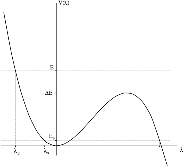
FIG. 6.: The potential $V(\lambda)$ for real $\lambda$. For later use, the energies $E_{0}$ and $E$ are also shown. $\psi_{0}$ has three turning points, and $\lambda=\lambda_{0}$ is the left-most of the three. $\psi_{E}$ has one turning point at $\lambda=\lambda_{E}$.

The soliton will decay if the $\lambda$ degree of freedom tunnels under the barrier given by the potential $V(\lambda)$ shown in Figure 6. The rate is of the form

$$\Gamma=Ce^{-2B}$$ (74)

where the factor $B$ is

$$B\,=\,\frac{\sqrt{2}}{\omega_{0}}\int_{0}^{3/2b}{\rm d}\lambda\sqrt{\lambda^{2}/2-b\lambda^{3}/3}\,=\,\frac{3}{5}\,\frac{1}{\omega_{0}b^{2}}\,=\,\frac{18}{5}\,\frac{\Delta E}{\omega_{0}}\ .$$ (75)

We are able to neglect the width of the wave function (73) in this calculation because as $g$ goes to zero it is small compared to the change in $\lambda$ during the tunnelling process. Since in the fixed $\Delta E$ limit $\omega_{0}\sim g^{1/3}$ we see that the tunnelling rate goes as $\exp(-{\rm constant}/g^{1/3})$. For the approximation to be reliable we require that $B$ be much greater than one. This in turn requires that $g$ be small.

We can compare this calculation with that of Rubakov, Stern and Tinyakov[13] who numerically calculated the action of the Euclidean space solution which tunnels under the barrier. They used the equations of motion of the full $3+1$ dimensional theory with the restriction to the spherical ansatz. At $\xi=12$ we have $\Delta E=1.2\,m/g^{2}$, $\omega_{0}=0.98\,m$ giving $g^{2}B=4.4$ which is to be compared with what we read off Figure 2 of Ref. [13], namely $g^{2}B=4\pm 1$. This agreement again supports the view that the $\lambda$ mode is the relevant degree of freedom for discussing soliton decay for $\xi$ near $\xi^{*}$.

We now turn to induced soliton decay. Our picture is that the soliton will decay if the $\lambda$-mode is excited to a state with energy above $\Delta E$. The $\lambda$-mode couples to the continuum modes $q_{\omega}$ which can bring energy from afar to the soliton. The free quantum Hamiltonian for the $q_{\omega}$ is

$$H_{q_{\omega}} = \frac{1}{2}\int_{m}d\omega\left[g^{2}p_{\omega}^{2}+\frac{\omega^{2}}{g^{2}}\,q_{\omega}^{2}\right]$$ (77)

$$= \int_{m}d\omega\,\omega\left[a_{\omega}^{\dagger}a_{\omega}+1/2\right]$$ (78)

where

$$a_{\omega}=\frac{1}{\sqrt{2\omega}}\left(\frac{\omega q_{\omega}}{g}+igp_{\omega}\right)\ .$$ (79)

The $q_{\omega}$ have been chosen to diagonalize the fluctuation matrix at the soliton. Therefore $H_{q_{\omega}}$ describes non-interacting massive $W$-bosons propagating in a fixed soliton background. For each value of $\omega$ there are actually an infinite number of different $W$-boson quanta. For example there are the states with frequency $\omega$ and all values of angular momentum relative to the soliton center. These extra labels are omitted throughout but their presence is understood.

The $\lambda$-mode couples to the continuum modes through cubic couplings of the form

$$H_{\rm int}=\frac{1}{\omega_{0}^{2}}\left\{\lambda^{2}\int_{m}d\omega\,d(\omega)\,q_{\omega}+\frac{\omega_{0}}{g}\lambda\int_{m}d\omega\,d\omega^{\prime}\,e(\omega,\omega^{\prime})\,q_{\omega}q_{\omega^{\prime}}\right\}$$ (80)

which appear in (61). We have rescaled $\lambda$ according to (69). The couplings (80) arose upon expanding about the soliton. The functions $d(\omega)$ and $e(\omega,\omega^{\prime})$ are peaked at values of $\omega$ corresponding to wavelengths of order the size of the soliton. They are also only peaked if the unspecified labels allow large overlap with the soliton. For example even with $\omega$ chosen so that $(\omega^{2}-m^{2})^{-1/2}\sim$ soliton size, it is only the low partial waves which have $d(\omega)$ and $e(\omega,\omega^{\prime})$ large.

The first term in (80) allows for the absorption of a single $W$-boson by the soliton. The $W$-boson energy $E$ is transferred to the $\lambda$-mode. The second term in (80) allows a single $W$-boson to scatter inelastically off the soliton, transferring energy $E$ to the $\lambda$-mode. We now calculate the rate for the absorption process; the calculation for the scattering process is similar. (The coefficients of the $\lambda$ and $\lambda^{2}$ operators have different $g$-dependence, but this will not affect the leading $g$-dependence of the cross-section for either process.) Assuming that the soliton starts in its ground state, in order for the soliton to decay we require $E+\omega_{0}/2>\Delta E$. Since $\omega_{0}\ll\Delta E$ we can approximate this as $E>\Delta E$. In the fixed $\Delta E$ limit we are free to choose $\Delta E$ to be a constant times $m$ where the constant is of order unity. (Recall that $m$ is held fixed throughout this paper.) Now the soliton size is roughly $2/(m\sqrt{\xi})$ and in the fixed $\Delta E$ limit $\xi$ goes to $\xi^{*}=10.35$. Thus the $W$-boson wavelength and the soliton size can be comparable. There is no length scale mismatch and $d(E)$ need not be small.

Using Fermi’s Golden Rule we now calculate the cross section for $W+{\rm soliton}\rightarrow$ anything with no soliton. Let $|{\bf k}\rangle$ be a single $W$-boson state with energy $E$, normalized to unit particle flux. Now

$$\langle 0|H_{\rm int}|{\bf k}\rangle=\frac{\lambda^{2}}{\omega_{0}^{2}}\,\int_{m}d\omega\,d(\omega)\,\langle 0|q_{\omega}|{\bf k}\rangle\equiv g\,\frac{\lambda^{2}}{\omega_{0}^{2}}\,\bar{d}({\bf k})\ ,$$ (81)

where we have defined $\bar{d}({\bf k})$ so that it is independent of $g$ (see (79)). The $\lambda$-mode starts in the state $\psi_{0}(\lambda)$ with energy $\sim\omega_{0}/2$ which again we neglect relative to $\Delta E$. The interaction (81) can cause a transition to a state $\psi_{E}(\lambda)$ in which the $\lambda$-mode has energy $E$. Since the width of $\psi_{0}$ is $\sim g^{1/6}\ll 1$, it is tempting to try approximating the states with $E>\Delta E$ as plane waves

$$\psi_{E}(\lambda)\sim\frac{1}{\omega_{0}^{1/2}E^{1/4}}\,\exp\left(i\sqrt{2E}\lambda/\omega_{0}\right)\ .$$ (82)

The cross section for a transition from $\psi_{0}$ to $\psi_{E}$ is

$$\sigma_{\rm destruction}={\cal N}\left(\frac{g\,\bar{d}({\bf k})}{\omega_{0}^{2}}\right)^{2}\ {\cal I}(E)^{2}\ ,$$ (83)

where ${\cal N}$ is a $g$-independent constant and where ${\cal I}(E)$ is the integral

$${\cal I}(E)=\int d\lambda\,\psi_{0}(\lambda)\,\lambda^{2}\,\psi_{E}(\lambda)\ .$$ (84)

If we take $\psi_{0}$ and $\psi_{E}$ as in (73) and (82) respectively, ${\cal I}(E)$ is easily evaluated, yielding

$${\cal I}(E)\sim\exp\left(-E/\omega_{0}\right)\ ,$$ (85)

where we have dropped all prefactors. This result is in fact incorrect. While it is true that (73) and (82) yield a good approximation to the integrand where the integrand is biggest, the result (85) is exponentially smaller than the integrand. This raises the possibility that corrections to the wave functions neglected to this point may change (85). We must, therefore, use WKB wave functions which take into account the quadratic and cubic terms in the potential $V(\lambda)$. As $g\rightarrow 0$ in the fixed $\Delta E$ limit, $\omega_{0}\rightarrow 0$ and using semi-classical wave functions becomes a better and better approximation. We show below that for $E=\Delta E$ the leading dependence of the of ${\cal I}(E)$ as $g\rightarrow 0$ in the fixed $\Delta E$ limit is in fact that of (85) with the coefficient of $\Delta E/\omega_{0}$ being $(18-4\sqrt{3})/5$ instead of $1$. Thus, we will find that even though the soliton destruction process does not involve tunnelling, the correct cross-section is exponentially small as $\omega_{0}\sim g^{1/3}$ goes to zero. The reader who is not interested in the details of the evaluation of ${\cal I}(E)$ can safely skip to equation (98).

We now wish to evaluate the leading semi-classical dependence of

$${\cal I}(E_{0},E)=\int d\lambda\,\psi_{E_{0}}\,\lambda^{2}\,\psi_{E}$$ (86)

in the fixed $\Delta E$ limit where $E>\Delta E$ and $\Delta E>E_{0}>0$ and where $\psi_{E}$ and $\psi_{E_{0}}$ are WKB wave functions for the Hamiltonian (70). See Figure 6. The reader may be concerned that (86) is infinite. (Both wave functions are real, and for large positive $\lambda$ the integrand (86) has a non-oscillatory piece which grows like $\lambda^{2}\lambda^{-3/2}$.) However, when the relevant limits are taken correctly, the answer we seek is in fact finite. Recall that our problem reduces to that of the $\lambda$ mode in a cubic potential only for $|\lambda|<\omega_{0}/g\sim g^{-2/3}$. Therefore, we should do the $\lambda$ integration from $\lambda=-\Lambda$ to $\lambda=+\Lambda$, where $\Lambda$ is real and positive and where we take $\Lambda$ to infinity more slowly than $g^{-2/3}$ as $g$ goes to zero. The result of such an evaluation would go like $\Lambda^{3/2}\exp(-{\rm constant}/\omega_{0})$. Because we do not take $\Lambda$ to infinity before taking $g$ to zero, the prefactor does not make the result infinite.

The evaluation of matrix elements of operators between semi-classical states has been treated by Landau[18], and although his final answer does not apply to our problem, we follow his method to its penultimate step. Landau’s method yields only the leading (i.e. exponential) dependence of such matrix elements, and says nothing about the prefactors. Thus, using Landau’s method yields the leading small-$g$ dependence of (86) irrespective of whether the prefactors make the integral infinite. In the calculation which follows, it nevertheless proves convenient to multiply the integrand in (86) by $\exp(-J\lambda^{2}/\omega_{0})$ with $J$ a constant. This does in fact render the integral finite, but it may also modify the exponential dependence of the result. Therefore, after the $g\rightarrow 0$ limit has been taken we must take the $J\rightarrow 0$ limit. Landau’s method[18] applied to our problem yields

$${\cal I}(E_{0},E)\sim{\rm Im} \Biggl{\{}\int d\lambda\,\frac{\omega_{0}\,\lambda^{2}}{\left[\left(V(\lambda)-E_{0}\right)\left(V(\lambda)-E\right)\right]^{1/4}}$$ (87)

$$\times \,\exp\Biggl{[}\frac{1}{\omega_{0}}\Biggl{(}\int_{\lambda_{0}}^{\lambda}dx\sqrt{2\left(V(x)-E_{0}\right)}-\int_{\lambda_{E}}^{\lambda}\,dx\,\sqrt{2\left(V(x)-E\right)}\,-J\lambda^{2}\,\Biggr{)}\Biggr{]}\Biggr{\}}\ .$$ (88)

In this expression, $\lambda$ is treated as complex and it is understood that the contour has been deformed into the upper half plane. This is done both in order to avoid the turning points on the real axis shown in Figure 7, and because in deriving (88) Landau uses expressions for WKB wave functions which are valid only in the upper half plane and not on the real axis. The first square root in the exponent in (88) is taken to be positive on the real axis for $\lambda<\lambda_{0}$ and the second is taken to be positive on the real axis for $\lambda<\lambda_{E}$.

The equation $V(x)-E=0$ has three roots. One is at $\lambda_{E}$, on the negative real axis, and the other two, at $\lambda_{\rm bp}$ and $\lambda_{\rm bp}^{*}$, have nonzero imaginary parts. (For $E\rightarrow\Delta E$, $\lambda_{\rm bp}$ goes to the real axis at $\lambda_{\rm sph}=1/b$.) In evaluating (88) we must keep in mind that at $\lambda=\lambda_{\rm bp}$ in the upper half plane, the integrand has a branch point. This singularity will play an important role in our analysis. (Unlike in the example treated explicitly by Landau, it does not arise from a singularity in $V(\lambda)$.) The branch cut from $\lambda_{\rm bp}$ must not cross the real axis, and it is convenient to take it to run upward vertically. The integrand in (88) is a function which is analytic in the upper half plane except at $\lambda_{\rm bp}$ and along the associated cut. To evaluate the integral, we are free to push the contour upward away from the real axis as long as we ensure that it does not touch the branch point $\lambda_{\rm bp}$ or cross the branch cut.

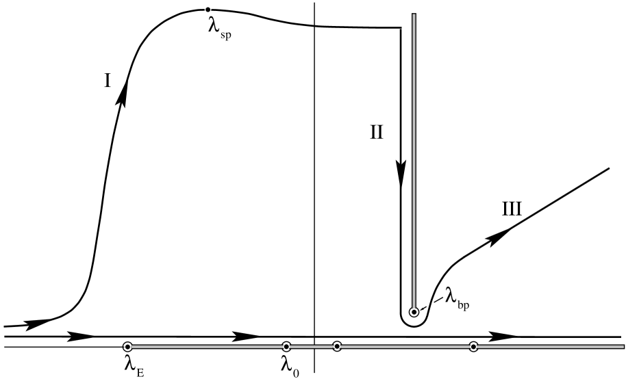
FIG. 7.: This figure is a sketch showing the important points in the complex $\lambda$-plane discussed in the text. The branch points are marked with dots, and the branch cuts are shaded. The contour in (5.19), just above the real axis, and the deformed contour we use to evaluate the integral are both shown.

We now evaluate the leading exponential dependence of (88). To this end, we drop the prefactors in (88). We write the integral as

$$\int d\lambda\,\exp\frac{1}{\omega_{0}}\Bigl{[}\,X(\lambda)+iY(\lambda)\,\Bigr{]}$$ (89)

where $X$ and $Y$ are real and where

$$X+i\,Y=\int_{\lambda_{0}}^{\lambda}\,dx\,\sqrt{2\left(V(x)-E_{0}\right)}-\int_{\lambda_{E}}^{\lambda}\,dx\,\sqrt{2\left(V(x)-E\right)}\,-J\lambda^{2}\ .$$ (90)

It is easy to check that for $J=0$ the integrand in (89) has no saddle points at finite $\lambda$. However, making $J$ nonzero introduces a saddle point at large $|\lambda|$ which moves off to infinity as $J$ is taken to zero and it is convenient for us to evaluate the integral with nonzero $J$ and then take the $J\rightarrow 0$ limit.

We now describe the behavior of $X$ at large $|\lambda|$. Write $\lambda=\Lambda\exp i\theta$. We have chosen the branch cut to run vertically and so it is at $\theta=\pi/2$ for large $\Lambda$. To the right of the cut, that is for $\pi/2>\theta>0$, as $\Lambda$ goes to infinity

$$X\sim-\Lambda^{5/2}\sin(5\theta/2)-J\Lambda^{2}\cos(2\theta)\ ,$$ (91)

and the $J$ term is subleading. $X$ goes to $+\infty$ at large $\Lambda$ for $\pi/2>\theta>2\pi/5$ and goes to $-\infty$ for $2\pi/5>\theta>0$. The descent to $-\infty$ is most rapid for $\theta=\pi/5$. To the left of the cut, that is for $\pi\geq\theta\geq\pi/2$, as $\Lambda$ goes to infinity

$$X\sim X^{*}+\Lambda^{-1/2}\sin(\theta/2)-J\Lambda^{2}\cos(2\theta)\ ,$$ (92)

where $X^{*}$ is a constant independent of $J$, $\Lambda$, and $\theta$. (For $J=0$, as $\Lambda$ goes to infinity for $\pi\geq\theta\geq\pi/2$, $X\rightarrow X^{*}$ and $Y\rightarrow 0$.) For nonzero $J$, there is a saddle point at finite $\lambda$. For small $J$, this saddle point is at $\theta\simeq 3\pi/5$ and $\Lambda\sim J^{-2/5}$. Thus, as $J\rightarrow 0$ the saddle point recedes to infinity as promised, and $J\Lambda^{2}$ at the saddle point goes to zero. Therefore, in the $J\rightarrow 0$ limit $X$ at the saddle point goes to the value $X^{*}$.

We now deform the contour as sketched in Figure 7. For nonzero $J$, the saddle point is at finite $\lambda$ and we choose the contour to follow the path of steepest descent from this saddle point. To the left of the saddle point, the steepest descent path curves toward the real axis, and then approaches the real axis asymptotically. As we discuss below, $X(\lambda_{\rm bp})$ is greater than $X^{*}$. Therefore, to the right of the saddle point, the path of steepest descent from the saddle point cannot get around the branch point and necessarily runs into the branch cut. After reaching the cut, the next section of the path ascends as it traverses (II), following the cut inward toward the origin, until it reaches the region of the branch point $\lambda_{\rm bp}$. Along (II), $X$ ascends monotonically from $X^{*}$ to $X(\lambda_{\rm bp})$. $Y$ is not constant. Then, to the right of the cut, the contour follows the path of steepest descent (III) toward infinity along $\theta=\pi/5$.

There are two contributions to the integral (89). First, the saddle point makes a contribution which goes like $\exp(X^{*}/\omega_{0})$. (Note that we take the $g\rightarrow 0$ limit and then take the $J\rightarrow 0$ limit.) The second contribution arises because the path must ascend from the saddle point at infinity as it traverses (II) in order to get around the branch point, before then descending along (III) to the right. Therefore, the integral (89) receives a contribution from the region of the branch point which goes like $\exp(X(\lambda_{\rm bp})/\omega_{0})$. In sum, therefore, the integral (88) goes like

$${\cal I}(E_{0},E)\sim\exp(X^{*}/\omega_{0})+\exp(X(\lambda_{\rm bp})/\omega_{0})\ ,$$ (93)

where we have dropped the prefactors, about which Landau’s method says nothing. At this point, we can take the $E_{0}\rightarrow 0$ and $E\rightarrow\Delta E$ limits simply by setting $E_{0}=0$ and $E=\Delta E$. Prior to this point in the calculation, taking these limits would require careful treatment of branch points. Henceforth we set $E_{0}=0$ and compute ${\cal I}(E)={\cal I}(0,E)$.

It only remains to evaluate the relative size of $X(\lambda_{\rm bp})$ and $X^{*}$. Both $X(\lambda_{\rm bp})$ and $X^{*}$ depend on $E$. After some calculation one finds that for $E=\Delta E$

$$X^{*}=-\omega_{0}B=-\frac{18}{5}\Delta E\ ,$$ (94)

where $B$ is the tunnelling amplitude computed in (75), and

$$X(\lambda_{\rm bp})=-\sqrt{2}\int_{0}^{1/b}{\rm d}\lambda\sqrt{\lambda^{2}/2-b\lambda^{3}/3}=-\frac{1}{5b^{2}}\left(3-\frac{2}{\sqrt{3}}\right)\,=\,-\frac{18}{5}\Delta E\left(1-\frac{2}{3\sqrt{3}}\right)\ ,$$ (95)

so $X(\lambda_{\rm bp})$ is the larger (i.e. least negative) of the two at $E=\Delta E$. At large $E$, both $X(\lambda_{\rm bp})$ and $X^{*}$ decrease like $-E^{5/6}$. For $E>\Delta E$, the integrals in (90) must be evaluated numerically. We find that both $X(\lambda_{\rm bp})$ and $X^{*}$ decrease monotonically with increasing energy, and $X(\lambda_{\rm bp})$ is always greater than $X^{*}$. Consequently, the integral is dominated by the region of the branch point for all energies $E\geq\Delta E$. That is,

$${\cal I}(E)\sim\exp(X(\lambda_{\rm bp})/\omega_{0})$$ (96)

and

$$\sigma_{\rm destruction}\sim\bar{d}^{2}({\rm k})\exp(2X(\lambda_{\rm bp})/\omega_{0})\ ,$$ (97)

where we have dropped all prefactors except $\bar{d}$. Thus, although the integrand has a saddle point (at infinity), the integral is not dominated by that saddle point. This occurs because the path of steepest descent from the saddle point necessarily runs into the branch cut. Equivalently, the presence of the branch cut prevents the actual contour of integration from being deformed into a path of steepest descent through the saddle point. Although the path can be deformed to pass through the saddle, it must ascend from the saddle to the region of the branch point. (Note that although $X(\lambda_{\rm bp})>X^{*}$ for all energies $E\geq\Delta E$, $X(\lambda_{\rm bp})$ is greater than $B\omega_{0}$, and the rate for induced soliton decay is greater than the tunnelling rate, only for $E$ within a range of energies which we determine numerically to be $\Delta E\leq E$ $\stackrel{{\scriptstyle{\textstyle<}}}{{{\textstyle\sim}}}$ $1.74\Delta E$.)

Because $X(\lambda_{\rm bp})$ decreases monotonically with increasing $E$, the cross section (97) for the soliton to be destroyed by a single $W$-boson is least suppressed by ${\cal I}(E)$ at threshold. For $E=\Delta E$ the soliton destruction cross section goes like

$$\sigma_{\rm destruction}\sim\bar{d}^{2}({\rm k})\exp\left(-\frac{36-8\sqrt{3}}{5}\Delta E/\omega_{0}\right)\$$ (98)

as $g\rightarrow 0$ in the fixed $\Delta E$ limit.

We expect $d(E)$ and accordingly $\bar{d}({\bf k})$ to be appreciable when $E\sim\Delta E$ so long as $\Delta E$ is comparable to the inverse soliton size, which is of order the inverse $W$-mass. Under these conditions, there will be no length scale mismatch and $d(E)$ will not depend sensitively on $E$ for $E\sim\Delta E$, so $\sigma_{\rm destruction}$ will be maximized for $E=\Delta E$. Thus the maximum rate for soliton decay induced by collision with a single $W$-boson is proportional to $\exp(-(36/5-8\sqrt{3}/5)\Delta E/\omega_{0})$. This is to be compared with the tunnelling rate in the same limit which is proportional to $\exp(-(36/5)\Delta E/\omega_{0})$. Both go to zero as $g$ goes to zero like $\exp(-{\rm constant}/g^{1/3})$, but the ratio of the tunnelling rate to the induced decay rate is exponentially small.

We have computed the cross section for a single $W$-boson to be absorbed by the soliton and to excite the $\lambda$-mode to a continuum state above the barrier, which in our picture results in soliton decay. The cross section for a $W$-boson to destroy the soliton by scattering off the soliton and transferring energy $E$ to the $\lambda$-mode can be calculated using the second term in (80). The calculation is similar to the one we have done and the result has the same exponential factor as in (98) but would have a different prefactor. Because the exponent in (98) includes $\omega_{0}^{-1}\sim g^{-1/3}$, these cross sections go to zero faster than any power of $g$ as $g$ goes to zero in the fixed $\Delta E$ limit. Note that this suppression arises even though the process does not involve tunnelling and even though there is no length scale mismatch. It arises as a consequence of the limit in which we have done the computation, because in that limit destroying the soliton reduces to exciting a single degree of freedom to an energy level infinitely many ($\sim\Delta E/\omega_{0}$) levels above its ground state. Thus, taking $g\rightarrow 0$ at fixed $\Delta E$ makes the computation tractable but makes the induced decay rate exponentially small, albeit larger than the tunnelling rate.

VI Fermion Number Violation

We have described classical and quantum processes in which electroweak solitons are destroyed. In this section, we argue that if we couple a quantized chiral fermion to the gauge and Higgs fields considered in this paper, then soliton destruction implies nonconservation of fermion number. The argument we present treats the gauge and Higgs fields as classical backgrounds. In particular, we ask how many fermions are produced in a background given by a solution to the classical equations of motion in which a soliton is destroyed. We expect that our conclusions will also be valid for soliton destruction induced by a single $W$-boson.

We introduce a quantized fermion field $\Psi$, and as in the standard electroweak theory but neglecting the $U(1)$ interaction, we couple only the left-handed component of the fermion to the non-Abelian gauge field. We add the usual Yukawa coupling between the fermion and the Higgs field to give the fermion a gauge invariant mass. The Lagrangian for the fermion is

$${\cal L}^{\rm fermion}=\bar{\Psi}\left[i\gamma^{\mu}D_{\mu}-m_{f}\,\left(UP_{R}+U^{\dagger}P_{L}\right)\right]\Psi\ ,$$ (99)

where $D_{\mu}=\partial_{\mu}-iA_{\mu}P_{L}$, $P_{L}=\frac{1}{2}(1-\gamma_{5})$ and $P_{R}=\frac{1}{2}(1+\gamma_{5})$. The Higgs field $\Phi$ of (2) is given by $\Phi=(v/\sqrt{2})U$. For simplicity, both the up and the down components of $\Psi$ have the same mass $m_{f}$. The gauge invariant normal ordered fermion current

$$J^{\mu}=\,:{\bar{\Psi}}\gamma^{\mu}\Psi:$$ (100)

is not conserved, that is,

$$\partial_{\mu}J^{\mu}=\frac{1}{32\pi^{2}}\,\epsilon^{\mu\nu\alpha\beta}\,{\rm Tr}\,\left(F_{\mu\nu}F_{\alpha\beta}\right)\ .$$ (101)

We consider backgrounds given by solutions of the kind found numerically in Section II. After the soliton has been destroyed the solution dissipates. By dissipation we mean that at late times the energy density approaches zero uniformly throughout space. This means that at late times the solutions are well described by solutions to the linearized equations of motion

$$\left(\partial_{\nu}\partial^{\nu}+m^{2}\right)A_{\mu}^{\rm lin}=0$$ (102)

in unitary gauge. It is tempting to try to integrate (101) and relate the fermion number violation to the topological charge

$$Q=\frac{1}{32\pi^{2}}\int d^{4}x\,\epsilon^{\mu\nu\alpha\beta}\,{\rm Tr}\,\left(F_{\mu\nu}F_{\alpha\beta}\right)\ .$$ (103)

First, note that because the region of space-time in which $F_{\mu\nu}\neq 0$ is not bounded, there is no reason to expect $Q$ to be an integer. Furthermore, it is shown in Ref. [19] that for a background which satisfies (102) at early and/or late times the integral in (103) is not absolutely convergent and $Q$ cannot sensibly be defined.

In a background given by a solution to the equations of motion which dissipates at early and late times, the number of fermions produced is known to be given by the change in Higgs winding number[19, 20]. In this paper, the Higgs mass is infinite so the Higgs winding number can never change. For solutions with no solitons in the initial or final states, the arguments of Ref. [19] apply, and no fermions are produced. However, if there is a soliton in the initial or final state the assumption of Ref. [19] that the solution dissipates is not satisfied. In this section, we show that in a background given by a solution in which one soliton is destroyed, one net anti-fermion is produced if the fermion is light ($m_{f}L\ll 1$ where $L$ is the size of the soliton) and no fermions are produced if the fermion is heavy ($m_{f}L\gg 1$). In the $m_{f}L\gg 1$ case, however, there is still a violation of fermion number in the sense that the soliton carries heavy fermion number whereas the dissipated configuration after the soliton is destroyed does not.

We now review some known facts about fermion charges which a background field configuration can carry[21, 9, 22]. Consider some localized time independent field configuration $A_{\mu}({\bf x})$ in the unitary gauge $U=1$. Imagine adiabatically interpolating from the trivial background $A_{\mu}({\bf x})=0$ to the $A_{\mu}({\bf x})$ of interest and following the adiabatic evolution of the fermion state which at the beginning of the interpolation is the fermion vacuum. At the beginning of the interpolation, the state has all negative energy levels filled with the mode functions determined by the single particle Dirac Hamiltonian

$$H_{\rm ferm}(t)=\gamma^{0}\left[-i\gamma^{i}D_{i}+m_{f}\,\right]-A_{0}P_{L}$$ (104)

with $A_{\mu}=0$. The change, from the beginning to the end of the interpolation, of the expectation of the fermion charge operator, $\int d^{3}{\bf x}\,J^{0}$ with $J^{0}$ given by (100), has been calculated[21]. The result is the Chern-Simons number of the field $A_{\mu}$

$$N_{\rm CS}[A]=\frac{1}{24\pi^{2}}\int d^{3}{\rm x}\epsilon^{ijk}\,{\rm Tr}\,\left[A_{i}A_{j}A_{k}+\frac{3}{2}\,iF_{ij}A_{k}\right]\ .$$ (105)

Since at the beginning of the interpolation the fermion charge is zero, $N_{\rm CS}$ is the charge of the state arrived at by adiabatically following the initial vacuum state. We will see that the fermion state reached by this adiabatic process is not necessarily the lowest energy fermion state in the background $A_{\mu}({\bf x})$.

Consider the case when the final configuration has the special form $A_{i}({\bf x})=iU_{1}^{\dagger}\partial_{i}U_{1}$, $A_{0}=0$ where $U_{1}$ is a winding number one map, say of the form (29), with a characteristic size $L$. In this case, $N_{\rm CS}[A]$ is the winding of $U_{1}$, that is $N_{\rm CS}[iU_{1}^{\dagger}\partial_{i}U_{1}]=1$. Thus the state arrived at at the end of the interpolation has fermion charge one. We now examine what this state is. At all times during the interpolation we can define an instantaneous single particle Dirac Hamiltonian by (104) and we can therefore discuss how the spectrum of the instantaneous Hamiltonian varies during the interpolation. At the beginning we have the free massive Dirac Hamiltonian which has a gap between $-m_{f}$ and $m_{f}$. If $m_{f}\gg 1/L$, then the spectrum is not perturbed much by the gauge field and in particular no energy levels cross zero during the interpolation. In this case, throughout the interpolation the fermion state is the lowest energy fermion state in the presence of the bosonic background. However if $m_{f}L\ll 1$, it has been shown[9] that one level crosses zero from below during the interpolation. This means that for $m_{f}L\ll 1$, the state reached at the end of the interpolation is the lowest energy fermion state in the presence of $A_{i}=iU_{1}^{\dagger}\partial_{i}U_{1}$ plus a single fermion. Thus the charge of the lowest energy fermion state in the presence of $A_{i}=iU_{1}^{\dagger}\partial_{i}U_{1}$ is zero for $m_{f}L\ll 1$. However for $m_{f}L\gg 1$, the charge of the lowest energy fermion state in this background is one. This ends our little review.

In the case at hand the electroweak soliton $A_{i}^{\rm sol}$ is only approximately of the form $iU_{1}^{\dagger}\partial_{i}U_{1}$ and the Chern-Simons number of the soliton configuration is not an integer. In fact a general background $A_{\mu}({\bf x})$ will not carry an integer-valued fermion charge and this charge can be viewed as a consequence of the polarization of the vacuum by the background. Nonetheless we will argue that when the soliton is destroyed an integer number of fermions is produced.

Consider a background given by a solution in which a soliton is destroyed. At $t=-T_{0}\ll 0$ the solution consists of a soliton at rest and an incoming pulse and at $t=T_{0}\gg 0$ there is only outgoing radiation. We wish to avoid evaluating the fermion charge at $t=\pm T_{0}$. To this end we introduce a background configuration $\bar{A}_{\mu}({\bf x},t)$ for $-T\leq t\leq T$ with $T>T_{0}$ which agrees with the solution $A_{\mu}({\bf x},t)$ for $-T_{0}\leq t\leq T_{0}$. At $t=-T$ we choose the background $\bar{A}_{\mu}({\bf x},-T)=iU_{1}^{\dagger}\partial_{i}U_{1}$ where $U_{1}$ is a winding number one map which produces a configuration which is close to the soliton, that is, $A_{i}^{\rm sol}\simeq iU_{1}^{\dagger}\partial_{i}U_{1}$. In particular the length scale over which $U_{1}$ varies, $L$, is determined by the size of the soliton. Thus the interpolation, running backward from $-T_{0}$, turns off the incoming pulse and distorts the soliton until it is of the form $iU_{1}^{\dagger}\partial_{i}U_{1}$. Now at $t=T_{0}$ the solution is just the outgoing remnants of the soliton and the initial pulse, and at $t=T$ we chose $\bar{A}_{\mu}({\bf x},T)=0$. Thus between $T_{0}$ and $T$ the interpolation turns off the outgoing pulse bringing the background to its vacuum configuration.

The interpolation $\bar{A}_{\mu}({\bf x},t)$ begins at $t=-T$ with a configuration of the form $\bar{A}_{i}({\bf x},-T)=iU_{1}^{\dagger}\partial_{i}U_{1}$ and ends at $\bar{A}_{\mu}({\bf x},T)=0$. The scale of $U_{1}$ is $L$. Consider a fermion field coupled to this background with $m_{f}L\gg 1$, the heavy fermion case. The initial gauge field configuration has heavy fermion number one. Consider the instantaneous Dirac Hamiltonian (104). Throughout the interpolation the gauge field $\bar{A}_{\mu}$ is small compared to $m_{f}$ and we conclude that no levels cross zero throughout the interpolation. Thus even without a detailed field theory description of fermion production we conclude that the fermion state we reach at the end of the interpolation has no extra heavy fermions. The final configuration is $\bar{A}_{\mu}({\bf x},T)=0$ so the fermion number of this gauge field configuration is zero. The heavy fermion number of the gauge field background has changed from one to zero and no heavy fermions have been produced and so we see an anomalous violation of heavy fermion number.

We now turn to the light fermion case, $m_{f}L\ll 1$. At $t=-T$ the configuration $\bar{A}_{i}({\bf x},-T)=iU_{1}^{\dagger}\partial_{i}U_{1}$ has light fermion number zero and we begin in the lowest energy fermion state in this background, which has all negative energy levels filled and all positive energy levels empty. Both the light and the heavy fermion number currents have the same anomalous divergence (101) so the difference between light and heavy fermion numbers is strictly conserved. We conclude that at $t=T$ the state we arrive at must have light fermion number minus one. The final configuration $\bar{A}_{\mu}({\bf x},T)=0$ has light fermion number zero. Thus we see that the fermion state at $t=T$ has one more light anti-fermion than light fermion. Thus in the background $\bar{A}_{\mu}$ between $t=-T$ and $t=T$ no heavy fermions are produced and one net light anti-fermion is produced.

We have discussed fermion production in a background going from $\bar{A}_{i}({\bf x},-T)=iU_{1}^{\dagger}\partial_{i}U_{1}$ to $\bar{A}_{i}({\bf x},T)=0$ whereas we are really interested in fermion production only in the presence of the solution $A_{\mu}({\bf x},t)$ for $-T_{0}\leq t\leq T_{0}$. Therefore we need to argue that no fermions are produced (light or heavy) between $-T$ and $-T_{0}$ and between $T_{0}$ and $T$. By making $T_{0}$ arbitrarily large, we can make the amplitude of the incident and outgoing pulses arbitrarily small, and so make their effect on the Dirac Hamiltonian arbitrarily small. This ensures that no fermions are produced during the interpolation between $T_{0}$ and $T$. It also ensures that, working backwards in time from $-T_{0}$, we can interpolate to a configuration with $\bar{A}_{\mu}=A_{\mu}^{\rm sol}$, removing the incident pulse, without producing any fermions.

It only remains to consider the interpolation between $\bar{A}_{i}({\bf x},-T)=iU_{1}^{\dagger}\partial_{i}U_{1}$ and $\bar{A}_{\mu}=A_{\mu}^{\rm sol}$. We can choose $U_{1}$ to be the winding number one map which characterizes the skyrmion with the same $e$ and $v$ as the soliton of interest. We can then choose the interpolating configurations to be a sequence of solitons with fixed $e$ and $v$ with $g$ changing from the value of interest to zero. The behavior of $\chi$ during such an interpolation is depicted in Figure 2. Note that in taking $g$ to zero with fixed $e$ and $v$, $\xi$ goes to infinity and $m$ goes to zero in such a way that the soliton size stays fixed. Note also that while we are choosing the configurations during the interpolation to be solitons with differing values of $g$, the coupling between the gauge field and the fermions is held fixed. For $m_{f}L\gg 1$, throughout the interpolation the fermion spectrum is not perturbed much by the gauge field, and so no levels cross zero. In our little review we learned that the configuration $iU_{1}^{\dagger}\partial_{i}U_{1}$ has fermion number one if $m_{f}L\gg 1$ and fermion number zero if $m_{f}L\ll 1$. Since $N_{\rm CS}[iU_{1}^{\dagger}\partial_{i}U_{1}]=1$ this means that as we reduce $m_{f}$ from $m_{f}\gg 1/L$ to $m_{f}\ll 1/L$ one (net) level must cross zero from below. Accordingly, for one or more values of $m_{f}$, of order $1/L$, the Dirac Hamiltonian (104) has a zero energy bound state in the skyrmion background and furthermore there is a nonzero value of $m_{f}$ below which there are no zero energy bound states. Now consider interpolating from the skyrmion configuration at $t=-T$ to the soliton configuration. Define $m_{f}^{*}(t)$ to be the largest value of $m_{f}$ such that for all $m_{f}<m_{f}^{*}(t)$ the Dirac Hamiltonian (104) in the background $\bar{A}_{\mu}({\bf x},t)$ does not have a zero energy bound state. From our understanding of the skyrmion background, we know that $m_{f}^{*}(-T)$ is of order $1/L$. By making $\xi$ arbitrarily large, the difference between the skyrmion and soliton configurations can be made arbitrarily small, and accordingly the change in the spectrum of the Dirac Hamiltonian during the interpolation can be made arbitrarily small. Therefore, for large enough $\xi$, throughout the interpolation from the skyrmion to the soliton $m_{f}^{*}(t)$ remains nonzero. We now assume that this is in fact the case for all $\xi>\xi^{*}$. We feel that this is a reasonable assumption since, as Figure 2 shows, the soliton configuration is quite similar to the corresponding skyrmion configuration even for $\xi$ near $\xi^{*}$. Making this assumption, we conclude that for $m_{f}L\ll 1$, as for $m_{f}L\gg 1$, no levels cross zero during the interpolation between $\bar{A}_{i}({\bf x},-T)=iU_{1}^{\dagger}\partial_{i}U_{1}$ and $\bar{A}_{\mu}=A_{\mu}^{\rm sol}$. Hence, no fermions (light or heavy) are produced during the interpolation between $-T$ and $-T_{0}$. Therefore, in the background between $-T_{0}$ and $T_{0}$, which is a classical solution in which a soliton is destroyed, no heavy fermions are produced and one net light anti-fermion is produced.

Suppose we are only interested light fermion production. We can view the heavy fermion as a device introduced only for the purpose of making an argument. Because we have not included the back reaction of the fermions, heavy or light, on the bosonic background, any conclusions we reach about the light fermion are in fact independent of whether there is or is not a heavy fermion in the theory. Therefore, in any process in which a soliton is destroyed, one net anti-fermion from each light $SU(2)_{L}$ doublet is anomalously produced.

VII Concluding Remarks

We have described a theory which agrees with the standard electroweak model at presently accessible energies but which includes a metastable soliton with mass of order several TeV. This Higgs sector soliton may have a dual description as a bound state particle made of more fundamental constituents or it may be that the Higgs sector is fundamental and when quantum effects are taken into account, a metastable soliton is found. In any event, given the soliton, under certain circumstances we can reliably estimate the rate for collision induced decays. The parameters of the theory can be chosen so that the soliton configuration is close to the sphaleron configuration, which means that using the soliton as an initial particle makes it easy to find sphaleron crossing processes. Indeed, we have found classical solutions in which the soliton is destroyed where the incoming pulse corresponds to a quantum coherent state with $\sim 1/g^{2}$ $W$-bosons. The rate for such processes is not exponentially suppressed as $g$ goes to zero. Furthermore in the limit $g$ goes to zero with $\Delta E=M_{\rm sph}-M_{\rm sol}$ fixed we can reliably estimate the rate for a two particle scattering process in which a single incident $W$-boson kicks the soliton over the barrier causing it to decay. We have argued that in all processes in which the soliton disappears fermion number is violated. This model may be relevant only as a theoretical foil, as a demonstration that fermion number violating high energy scattering processes can be very different than in the standard model. However if no light Higgs boson is discovered, it is even possible that Nature may be described by such a model.

A

In Section II, we presented the equations of motion in the spherical ansatz in the unitary gauge. In this appendix, we begin by presenting the action and equations of motion in the spherical ansatz without fixing a gauge. All the numerical solutions presented in this paper were obtained by solving both the unitary gauge equations of motion and the $A_{0}=0$ gauge equations of motion using different numerical schemes. We sketch both methods in this appendix.

The spherical ansatz is given by expressing the gauge field $A_{\mu}$ and the Higgs field $\Phi$ in terms of six real functions $a_{0}\,,\,a_{1}\,,\,\alpha\,,\gamma\,,\mu\ {\rm and}\ \nu\ {\rm of}\ r\ {\rm and}\ t$. $A_{\mu}$ is given in (16) and $\Phi$ is given by

$$\Phi({\bf x},t)=\frac{1}{g}\left[\mu(r,t)+i\nu(r,t){\kern-0.24994pt\hbox{$\sigma$}\kern-5.71413pt\kern 0.50003pt\hbox{$\sigma$}\kern-5.71413pt\kern-0.24994pt\raise 0.43304pt\hbox{$\sigma$}}\cdot{\bf\hat{x}}\right]\ .$$ (A1)

For $A_{\mu}$ and $\Phi$ to be regular at the origin, we require that $a_{0}$, $\alpha$, $a_{1}-\alpha/r$, $\gamma/r$ and $\nu$ vanish as $r\to 0$. It is convenient to define the complex field

$$\phi=\mu+i\nu\ .$$ (A2)

When the Higgs mass is set to infinity, $|\phi|$ is frozen at its vacuum expectation value $\sqrt{2}m$ and

$$\phi=\sqrt{2}\,m\,\exp i\eta(r,t)\ ,$$ (A3)

with $\eta$ vanishing at the origin. Under a gauge transformation of the form $\exp[i\Omega(r,t){\kern-0.24994pt\hbox{$\sigma$}\kern-5.71413pt\kern 0.50003pt\hbox{$\sigma$}\kern-5.71413pt\kern-0.24994pt\raise 0.43304pt\hbox{$\sigma$}}\cdot{\bf\hat{x}}/2]$ with $\Omega(0,t)=0$, configurations in the spherical ansatz remain in the spherical ansatz and continue to satisfy the appropriate boundary conditions at the origin. Thus, the $SU(2)$ gauge theory reduced to the spherical ansatz has a residual $U(1)$ gauge invariance.

In the spherical ansatz the action associated with the Lagrangian (8) takes the form

$$S=\frac{4\pi}{g^{2}}\int dt\int^{\infty}_{0}dr\, \Bigg{\{}-\frac{1}{4}r^{2}f^{\mu\nu}f_{\mu\nu}+\left(D^{\mu}\chi\right)^{*}D_{\mu}\chi+2r^{2}m^{2}\,\left(\partial_{\mu}\eta-\frac{1}{2}a_{\mu}\right)^{2}$$ (A6)

$$-\frac{1}{2r^{2}}\left(~{}|\chi|^{2}-1\right)^{2}-m^{2}\left(|\chi|^{2}+1\right)-2m^{2}\,{\rm Re}\left(i\chi^{*}{\rm e}^{2i\eta}\right)$$

$$-\frac{1}{4\xi}G(\chi,\eta)\left[-4\left(\partial_{\mu}\eta-\frac{1}{2}a_{\mu}\right)^{2}+\frac{1}{2r^{2}}G(\chi,\eta)\right]\Bigg{\}}\ ,$$

where

$$G(\chi,\eta)=\left|\chi+i{\rm e}^{2i\eta}\right|^{2}$$ (A7)

and the rest of the notation is as in Section II. The notation is chosen to manifest the $U(1)$ gauge invariance present in the action (A6). The complex scalar fields $\chi$ and $\phi$ have $U(1)$ charges of $1$ and $1/2$ respectively, $a_{\mu}$ is the $U(1)$ gauge field, $f_{\mu\nu}$ is the field strength, and $D_{\mu}$ is the covariant derivative. The indices are raised and lowered with the $1+1$ dimensional metric $ds^{2}=dt^{2}-dr^{2}$.

The equations of motion in the spherical ansatz are

$$\partial^{\mu}(r^{2}f_{\mu\nu})=i\left[\chi D_{\nu}\chi^{*}-\chi^{*}D_{\nu}\chi\right]+\left(\partial_{\nu}\eta-\frac{1}{2}a_{\nu}\right)\left(2r^{2}m^{2}+\frac{1}{\xi}G(\chi,\eta)\right)$$ (A9)

$$\Bigg{[}D^{2}+\frac{1}{r^{2}}(|\chi|^{2}-1) +m^{2}~{}\Bigg{]}\chi$$ (A11)

$$=-i\,m^{2}{\rm e}^{2i\eta}-\frac{1}{4\xi}\left(\chi+i{\rm e}^{2i\eta}\right)\left[-4\left(\partial_{\mu}\eta-\frac{1}{2}a_{\mu}\right)^{2}+\frac{1}{r^{2}}G(\chi,\eta)\right]$$

$$\partial_{\mu}\Bigg{[}\bigg{(}r^{2}+\frac{1}{2m^{2}\xi} G(\chi,\eta)\bigg{)}\left(\partial^{\mu}\eta-\frac{1}{2}a^{\mu}\right)\Bigg{]}$$ (A13)

$$={\rm Re}\left(\chi^{*}{\rm e}^{2i\eta}\right)+\frac{1}{4m^{2}\xi}\,{\rm Re}\left(\chi^{*}{\rm e}^{2i\eta}\right)\left[-4\left(\partial_{\mu}\eta-\frac{1}{2}a_{\mu}\right)^{2}+\frac{1}{r^{2}}G(\chi,\eta)\right]$$

The same equations are obtained either by varying the action (8) and then imposing the spherical ansatz or by varying the action (A6). The unitary gauge action and the equations of motion of Section II are obtained by setting $\eta=0$. As a consequence of the $U(1)$ gauge invariance, the five equations above are not independent, and in Section II we chose to discard (A13).

In presenting the results of Section II, we found it useful to use the variables $\rho$, $\theta$, and $a_{1}$. The first is explicitly gauge invariant. The latter two are specific to the unitary gauge, and are equivalent to the gauge invariant variables $(\theta-2\eta)$ and $(a_{1}-2\partial_{1}\eta)$. For an extensive discussion of gauge invariant variables in the spherical ansatz, see Ref. [23].

In the simulations of Section II, the boundary conditions at the large-$r$ boundary of the lattice are not important, since we are interested in an ingoing pulse and its effects on the soliton and we stop the simulation before the remnants of the soliton reach the large-$r$ boundary. In doing the simulation in Figure 5 of Section IV, we must have energy absorbing boundary conditions at the large $r$ boundary of the simulation so that we can see the amplitude of the $\lambda$ mode oscillation decrease as it radiates energy away. At large radius, $\chi$ satisfies $\left[\partial^{2}/\partial t^{2}-\partial^{2}/\partial r^{2}-m^{2}\right]\chi(r,t)=0$. We choose to impose $\dot{\chi}=-\partial\chi/\partial r$ at the large $r$ boundary. This has the virtue that the energy flux at the boundary is never negative — the boundary can only absorb energy and cannot emit it.

We now give brief descriptions of the methods we used to solve the unitary gauge and $A_{0}=0$ gauge equations. In $A_{0}=0$ gauge, we chose to write a lattice version of the action (A6) and vary it, thus obtaining discretized versions of the equations of motion. The fields $\chi$ and $\eta$ live at the sites of the lattice, while $a_{1}$ lives on the spatial links. For a more detailed description of this technique as applied to the $1+1$ dimensional Abelian Higgs model, see Refs. [24, 25]. In the $A_{0}=0$ gauge, we have the freedom to make a time-independent gauge transformation and we used this to set $\eta(r,0)=0$. However, $\eta$ does not remain zero at later times. We specified initial conditions for $\chi$, $\dot{\chi}$, $a_{1}$ and $\dot{\eta}$ at $t=0$, and then chose initial values for $\dot{a}_{1}$ such that Gauss’ law is satisfied. The equations of motion are second order in time derivatives of the fields $\chi$, $a_{1}$ and $\eta$. We used the fields at two successive time steps to determine the fields at the next time step. We used a lattice with $4000$ sites and a lattice spacing $dr=0.004/m$, and used a time step $dt=dr/2$. Because the equations of motion were obtained by varying a lattice action, there is a lattice version of Gauss’ law which is satisfied during the evolution up to the precision allowed by computer arithmetic. Energy conservation was satisfied throughout the evolution to better than one part in a thousand. We verified that reducing $dr$ and $dt$ did not change any results quantitatively, and reduced the violation of energy conservation. We also checked that if we take the final configuration from a simulation like that of Figure 3, change the sign of all time derivatives, and run the simulation backwards in time, we obtain the initial configuration of the original simulation.

With the unitary gauge equations of motion, we followed a different strategy. We first wrote them as first order equations for $a_{0}$, $a_{1}$, $\chi$, and the canonical momenta $\Pi_{a_{1}}$ and $\Pi_{\chi}$. Of these seven equations, one is redundant. In doing the numerical evolution it was convenient to drop the equation for $\dot{\Pi}_{a_{1}}$. We therefore chose initial conditions by specifying $\chi$, $a_{1}$, $a_{0}$, and $\Pi_{\chi}$, and then chose $\Pi_{a_{1}}$ such that Gauss’ law was satisfied. Rather than using a lattice action, we discretized the equations of motion themselves. We took care, however, to put $\chi$, $\Pi_{\chi}$ and $a_{0}$ at the lattice sites while putting $a_{1}$ and $\Pi_{a_{1}}$ on the links, and to discretize the equations of motion in such a way that all quantities were accurate to one order in $dr$ beyond the trivial one. We implemented the time evolution using a fourth order Runge-Kutta algorithm. We worked with a lattice spacing of $dr=0.02/(m\sqrt{\xi})$, equal to $0.0058/m$ for $\xi=12$, and a time spacing $dt=0.002/m$. We verified that energy conservation and the equation for $\dot{\Pi}_{a_{1}}$ were satisfied. For smaller $dr$ and $dt$, no qualitative changes occurred and both checks were satisfied more accurately.

B Classical Solutions and Coherent States

There is clearly a relation between classical solutions in Minkowski space and the tree approximation in quantum field theory[26]; in this section we derive a version of this relation useful for our purpose. This appendix is self-contained and can be read independently of the rest of this paper.

For simplicity, consider real scalar field theory with the action

$$S=\frac{1}{g^{2}}\int{\rm d}^{4}x\left\{\frac{1}{2}\,\partial_{\mu}\phi\,\partial^{\mu}\phi-\frac{1}{2}\,m^{2}\phi^{2}-V(\phi)\right\}$$ (B1)

where $V(\phi)$ is a polynomial containing cubic and higher terms. The classical field equation,

$$\left(\partial^{2}+m^{2}\right)\phi_{c}(x)+V^{\prime}\Big{(}\phi_{c}(x)\Big{)}=0$$ (B2)

is equivalent to the integral equation

$$\phi_{c}(x)=F_{\rm in}(x)+F^{*}_{\rm out}(x)-i\int D_{F}(x-y)V^{\prime}\Big{(}\phi_{c}(y)\Big{)}{\rm d}^{4}y$$ (B3)

where

$$D_{F}(x)=-\,\frac{1}{(2\pi)^{4}\,i}\int{\rm d}^{4}k\,\frac{e^{-ikx}}{k^{2}-m^{2}+i\epsilon}$$ (B4)

is the Feynman propagator and

$$F_{\stackrel{{\scriptstyle\rm{\scriptstyle in}}}{{\rm{\scriptstyle out}}}}(x)=\int{\rm d}k\,f_{\stackrel{{\scriptstyle\rm{\scriptstyle in}}}{{\rm{\scriptstyle out}}}}({\bf k})e^{-ikx}\ .$$ (B5)

In (B5), $k^{0}=|\sqrt{{\bf k}^{2}+m^{2}}|$ and ${\rm d}k$ is the Lorentz invariant measure

$${\rm d}k=\frac{1}{(2\pi)^{3}}\,\frac{1}{2k^{0}}\,{\rm d}^{3}{\bf k}$$ (B6)

We do not yet require that $\phi_{c}(x)$ is real. $f_{\rm in}$ and $f_{\rm out}$ are then arbitrary complex functions of ${\bf k}$.

Equation (B3) can be solved by iteration, and the solution expressed as a sum of terms described by Feynman diagrams. A typical diagram (for $V(\phi)=\frac{1}{6}\phi^{3}$) is shown in Figure B1.

FIG. B1

Its contribution to $\phi_{c}(x)$ is

$$\frac{1}{2}\int{\rm d}^{4}y\,{\rm d}^{4}z\,(-i)^{2}D_{F}(x-y)D_{F}(y-z)\left\{F^{*}_{\rm out}(z)\right\}^{2}F_{\rm in}(y)\ .$$ (B7)

The sum is over all connected, tree diagrams. The combinatorial factors are determined by the symmetry of the diagrams in the usual way.

We now ask which quantity in the quantum field theory with action (B1) is given in tree approximation by the same set of diagrams. The answer is

$$\phi_{c}(x)=\langle\hat{\phi}(x)\rangle_{f,{\rm tree}}\equiv\left[\frac{\left\langle f_{\rm out}\right|\hat{\phi}(x)\left|f_{\rm in}\right\rangle}{\langle f_{\rm out}|f_{\rm in}\rangle}\right]_{\rm tree}$$ (B8)

where $\Big{|}f_{\stackrel{{\scriptstyle\rm{\scriptstyle in}}}{{\rm{\scriptstyle out}}}}\Big{\rangle}$ are coherent states defined by

$$\Big{|}f_{\stackrel{{\scriptstyle\rm{\scriptstyle in}}}{{\rm{\scriptstyle out}}}}\Big{\rangle}=\sum_{n}\frac{1}{g^{n}n!}\,\int f_{\stackrel{{\scriptstyle\rm{\scriptstyle in}}}{{\rm{\scriptstyle out}}}}({\bf k}_{1}){\rm d}{\bf k}_{1}\ldots f_{\stackrel{{\scriptstyle\rm{\scriptstyle in}}}{{\rm{\scriptstyle out}}}}({\bf k}_{n}){\rm d}{\bf k}_{n}\Big{|}{\bf k}_{1}\ldots{\bf k}_{n};{\stackrel{{\scriptstyle\rm{\scriptstyle in}}}{{\rm{\scriptstyle out}}}}\Big{\rangle}$$ (B9)

where $\left|{\bf k}_{1}\ldots{\bf k}_{n};{\stackrel{{\scriptstyle\rm{\scriptstyle in}}}{{\rm{\scriptstyle out}}}}\right\rangle$ are the usual asymptotic $n$-particle states. In terms of the quantum field $\hat{\phi}(x)$,

$$\Big{|}f_{\stackrel{{\scriptstyle\rm{\scriptstyle in}}}{{\rm{\scriptstyle out}}}}\Big{\rangle}=\biggl{[}\exp\frac{i}{g^{2}}\lim_{x^{0}\rightarrow\mp\infty}\int{\rm d}^{3}x\biggl{\{}F_{\stackrel{{\scriptstyle\rm{\scriptstyle in}}}{{\rm{\scriptstyle out}}}}(x)\biggl{(}\frac{\overrightarrow{\partial}}{\partial x^{0}}-\frac{\overleftarrow{\partial}}{\partial x^{0}}\biggr{)}\hat{\phi}(x)\biggr{\}}\biggr{]}\Big{|}0\Big{\rangle}\ .$$ (B10)

Note that with our definitions of $S$ and $\left|f\right\rangle$, both sides of (B8) are independent of $g$. The one-loop corrections to $\left\langle\hat{\phi}(x)\right\rangle_{f}$ are of order $g^{2}$. Note also the normalizations

$${\bf I}=\sum_{n}\frac{1}{n!}\int{\rm d}{\bf k}_{1}\ldots{\rm d}{\bf k}_{n}\left|{\bf k}_{1}\ldots{\bf k}_{n}\right\rangle\left\langle{\bf k}_{1}\ldots{\bf k}_{n}\right|$$ (B11)

and

$$\langle{\bf k}|\hat{\phi}(x)|0\rangle = g\,e^{ikx}$$ (B12)

$$\Big{\langle}0\Big{|}f_{\stackrel{{\scriptstyle\rm{\scriptstyle in}}}{{\rm{\scriptstyle out}}}}\Big{\rangle} = 1$$ (B13)

$$\Big{\langle}f_{\stackrel{{\scriptstyle\rm{\scriptstyle in}}}{{\rm{\scriptstyle out}}}}\Big{|}f_{\stackrel{{\scriptstyle\rm{\scriptstyle in}}}{{\rm{\scriptstyle out}}}}\Big{\rangle} = \exp\frac{1}{g^{2}}\int\Big{|}f_{\stackrel{{\scriptstyle\rm{\scriptstyle in}}}{{\rm{\scriptstyle out}}}}\Big{|}^{2}{\rm d}k\ .$$ (B14)

It is important to note that the number of particles in the states $|f\rangle$ is of order $1/g^{2}$.

There is certainly a large class of solutions $\phi_{c}(x)$ which behave at early and late times like incoming and outgoing wave solutions of the free field equation, with amplitudes which go to zero at early and late times because of both the spread in $3$-space and the dispersion due to $m\neq 0$. For such solutions, with $f_{\stackrel{{\scriptstyle\rm{\scriptstyle in}}}{{\rm{\scriptstyle out}}}}$ smooth enough, we have

$$x^{0}\rightarrow-\infty,~{}~{}~{}~{}\phi_{c}(x) \sim \int{\rm d}k\,f_{\rm in}({\bf k})e^{-ikx}+\int{\rm d}k\,h^{*}_{\rm in}({\bf k})e^{ikx}$$ (B16)

$$x^{0}\rightarrow+\infty,~{}~{}~{}~{}\phi_{c}(x) \sim \int{\rm d}k\,h_{\rm out}({\bf k})e^{-ikx}+\int{\rm d}k\,f^{*}_{\rm out}({\bf k})e^{ikx}$$ (B17)

where, using (B3) and the values of $D_{F}(x-y)$ as $x^{0}\rightarrow\mp\infty$,

$$h^{*}_{\rm in}({\bf k}) = f^{*}_{\rm out}({\bf k})-i\int{\rm d}^{4}y\,e^{-iky}V^{\prime}\Big{(}\phi_{c}(y)\Big{)}$$ (B19)

$$h_{\rm out}({\bf k}) = f_{\rm in}({\bf k})-i\int{\rm d}^{4}y\,e^{iky}V^{\prime}\Big{(}\phi_{c}(y)\Big{)}\ .$$ (B20)

With a given complex $\phi_{c}(x)$, we read off $f_{\rm in}({\bf k})$ from the positive frequency part as $x^{0}\rightarrow-\infty$, and $f^{*}_{\rm out}({\bf k})$ from the negative frequency part as $x^{0}\rightarrow+\infty$ to discover what $\phi_{c}(x)$ is the tree approximation to. If $\phi_{c}(x)$ is real,

$$h_{\stackrel{{\scriptstyle\rm{\scriptstyle in}}}{{\rm{\scriptstyle out}}}}({\bf k})=f_{\stackrel{{\scriptstyle\rm{\scriptstyle in}}}{{\rm{\scriptstyle out}}}}({\bf k})$$ (B21)

and equations (B) become equivalent relations which determine $f_{\rm out}({\bf k})$ in terms of $f_{\rm in}({\bf k})$. Of course we are concerned with given real solutions $\phi_{c}(x)$ and we simply read off both $f_{\rm in}$ and $f_{\rm out}$ from the asymptotic behavior; we do not need equations (B) to relate them.

Returning to the complex case, we derive an expression for the matrix element $\left\langle f_{\rm out}\big{|}f_{\rm in}\right\rangle$ in the tree approximation in terms of the corresponding $\phi_{c}$. The quantum perturbation theory gives

$$\left\langle f_{\rm out}\big{|}f_{\rm in}\right\rangle=\exp\frac{1}{g^{2}}\,T(f_{\rm out},f_{\rm in})$$ (B22)

with $T$ expressed as the sum of connected Feynman diagrams. A typical tree diagram (again, for $V(\phi)=\frac{1}{6}\phi^{3}$) is shown in Figure B2.

FIG. B2

This contributes

$$\frac{(-i)^{3}}{2}\int D_{F}(x-y)D_{F}(y-z)\left\{F_{\rm in}(x)\right\}^{2}F^{*}_{\rm out}(y)F_{\rm in}(z)F^{*}_{\rm out}(z){\rm d}^{4}x\,{\rm d}^{4}y\,{\rm d}^{4}z$$ (B23)

to $T(f_{\rm out},f_{\rm in})$. Now consider small changes $\delta f_{\stackrel{{\scriptstyle\rm{\scriptstyle in}}}{{\rm{\scriptstyle out}}}}$. It can be seen that

$$\delta T(f_{\rm out},f_{\rm in}) = \int{\rm d}k\,\delta f^{*}_{\rm out}({\bf k})\left\{f_{\rm in}({\bf k})+i\int{\rm d}^{4}y\,e^{iky}\left(\partial^{2}+m^{2}\right)\langle\hat{\phi}(y)\rangle_{f}\right\}$$ (B25)

$$+\,\int{\rm d}k\,\delta f_{\rm in}({\bf k})\left\{f^{*}_{\rm out}({\bf k})+i\int{\rm d}^{4}y\,e^{-iky}\left(\partial^{2}+m^{2}\right)\langle\hat{\phi}(y)\rangle_{f}\right\}$$

where

$$\langle\hat{\phi}(x)\rangle_{f}=\frac{\left\langle f_{\rm out}\right|\hat{\phi}(x)\left|f_{\rm in}\right\rangle}{\langle f_{\rm out}|f_{\rm in}\rangle}\ .$$ (B26)

In the tree approximation, using (B8), (B2) and (B),

$$\delta T_{\rm tree}(f_{\rm out},f_{\rm in})=\int{\rm d}k\,\left\{\delta f^{*}_{\rm out}({\bf k})h_{\rm out}({\bf k})+\delta f_{\rm in}({\bf k})h^{*}_{\rm in}({\bf k})\right\}\ .$$ (B27)

We can now verify that (B27) is satisfied by

$$T_{\rm tree}(f_{\rm out},f_{\rm in}) = \frac{1}{2}\int{\rm d}k\,f^{*}_{\rm out}({\bf k})h_{\rm out}({\bf k})+\frac{1}{2}\int{\rm d}k\,f_{\rm in}({\bf k})h^{*}_{\rm in}({\bf k})$$ (B29)

$$-i\int{\rm d}^{4}x\,\left[\frac{1}{2}\phi_{c}(x)\left\{(\partial^{2}+m^{2})\phi_{c}(x)\right\}+V\Big{(}\phi_{c}(x)\Big{)}\right]\ .$$

Of course (B29) is $i$ times the classical action plus boundary terms. The point of the preceding argument is to get the boundary terms right. The expression (B29) can also be derived from the stationary value of a functional integral expression for $\langle f_{\rm out}|f_{\rm in}\rangle$. Note that the integral over space-time can be written as

$$\theta=\int{\rm d}^{4}x\,\left[V\Big{(}\phi_{c}(x)\Big{)}-\frac{1}{2}\phi_{c}(x)V^{\prime}\Big{(}\phi_{c}(x)\Big{)}\right]$$ (B30)

and so converges for typical solutions $\phi_{c}(x)$ which fall off rapidly enough in both space and time.

Now consider $f_{\stackrel{{\scriptstyle\rm{\scriptstyle in}}}{{\rm{\scriptstyle out}}}}$ which correspond to a real solution $\phi_{c}(x)$. Then (using (B22)),

$$\left\langle f_{\rm out}\big{|}f_{\rm in}\right\rangle_{\rm tree}=\exp\left[\frac{1}{2g^{2}}\int\left|f_{\rm out}\right|^{2}{\rm d}k+\frac{1}{2g^{2}}\int\left|f_{\rm in}\right|^{2}{\rm d}k-\frac{i\theta}{g^{2}}\right]$$ (B31)

where $\theta$ given by (B30) is real. Using (B14), we see that

$$\frac{\left|\left\langle f_{\rm out}\big{|}f_{\rm in}\right\rangle_{\rm tree}\right|^{2}}{\left\langle f_{\rm out}\big{|}f_{\rm out}\right\rangle\left\langle f_{\rm in}\big{|}f_{\rm in}\right\rangle}=1\ .$$ (B32)

One-loop corrections to $T(f_{\rm out},f_{\rm in})$ are of order $g^{2}$. Thus if we consider states

$$\Big{|}\tilde{f}_{\stackrel{{\scriptstyle\rm{\scriptstyle in}}}{{\rm{\scriptstyle out}}}}\Big{\rangle}=\frac{\Big{|}f_{\stackrel{{\scriptstyle\rm{\scriptstyle in}}}{{\rm{\scriptstyle out}}}}\Big{\rangle}}{\Big{\langle}f_{\stackrel{{\scriptstyle\rm{\scriptstyle in}}}{{\rm{\scriptstyle out}}}}\Big{|}f_{\stackrel{{\scriptstyle\rm{\scriptstyle in}}}{{\rm{\scriptstyle out}}}}\Big{\rangle}^{1/2}}$$ (B33)

normalized to unity,

$$\left|\tilde{f}_{\rm in}\right\rangle=e^{-i\theta/g^{2}}\,a\,\left|\tilde{f}_{\rm out}\right\rangle+|\psi\rangle$$ (B34)

where $\left\langle\psi\Big{|}\tilde{f}_{\rm out}\right\rangle=0$ and $|a|$ is not of order $\exp(-c/g^{2})$ as $g\rightarrow 0$. In fact (not proved here) to order $g^{0}$, i.e. one loop,

$$|a|^{2}=e^{-P}$$ (B35)

where $P$ is the probability of the transition vacuum $\rightarrow$ one pair of $\phi$ particles in the theory with action

$$S^{\prime}=\frac{1}{2}\int{\rm d}^{4}x\left\{\partial_{\mu}\phi\,\partial^{\mu}\phi-m^{2}(x)\phi^{2}\right\}$$ (B36)

where

$$m^{2}(x)=m^{2}+V^{\prime\prime}(\phi_{c}(x))\ .$$ (B37)

Thus, to each real solution $\phi_{c}(x)$ to the Minkowski space classical equations of motion, there corresponds a not exponentially suppressed scattering process between coherent states (containing of order $1/g^{2}$ particles).

REFERENCES

- [1] G. ’t Hooft, Phys. Rev. Lett. 37, 8 (1976); Phys. Rev. D 14, 3432 (1976); ibid 18, 2199 (1978).
-
[2]
N. Manton, Phys. Rev. D 28 2019, 1983;
F. Klinkhamer and N. Manton, Phys. Rev. D 30 2212, 1984. - [3] For example, see R. L. Singleton, Jr., L. Susskind and L. Thorlacius, Nucl. Phys. B343, 541 (1990); and T. Banks, G. Farrar, M. Dine, D. Karabali and B. Sakita, ibid. B347, 581 (1990).
-
[4]
A. Ringwald, Nucl. Phys. B330, 1 (1990); O. Espinosa
ibid. B343, 310 (1990).
For a review, see M. P. Mattis, Phys. Rep. 214, 159 (1992). -
[5]
V. A. Kuzmin, V. A. Rubakov and M. E. Shaposhnikov,
Phys. Lett. 155B, 36 (1985);
P. Arnold and L. McLerran, Phys. Rev. D 36, 581 (1987).
For reviews, see N. Turok, in Perspectives in Higgs Physics, G. Kane, ed., World Scientific, 300 (1992); and A. Cohen, D. Kaplan and A. Nelson, Ann. Rev. Nucl. Part. Phys. 43, 27 (1993). - [6] T. H. R. Skyrme, Proc. Roy. Soc. A260, 127 (1961).
-
[7]
J. M. Gipson and H. C. Tze, Nucl. Phys. B183, 524 (1981);
J. M. Gipson, ibid B231, 365 (1984). - [8] E. D’Hoker and E. Farhi, Phys. Lett. 134B, 86 (1984).
- [9] E. D’Hoker and E. Farhi, Nucl. Phys. B241, 109 (1984).
-
[10]
J. Ambjorn and V. A. Rubakov, Nucl. Phys. B256,
434 (1985);
V. A. Rubakov, Nucl. Phys. B256, 509 (1985). - [11] E. Witten, Nucl. Phys. B223, 422 (1983); ibid, B223, 433 (1983).
- [12] G. S. Adkins, C. R. Nappi and E. Witten, Nucl. Phys. B228, 552 (1983).
- [13] V. A. Rubakov, B. E. Stern and P. G. Tinyakov, Phys. Lett. 160B, 292 (1985).
-
[14]
E. Witten, Phys. Rev. Lett. 38, 121 (1977);
B. Ratra and L.G. Yaffe, Phys. Lett. B205, 57 (1988). - [15] C. Rebbi and R. Singleton, Jr., Numerical Investigation of Baryon Non-Conserving Processes in the Electroweak Theory, BU-HEP-95-5, hep-ph/9502370 (1995).
- [16] J. Goldstone and R. Jackiw, Phys. Rev. D 11, 1486 (1975).
- [17] Y. Brihaye and J. Kunz, Z. Phys. C41 (1989) 663.
- [18] L. D. Landau and E. M. Lifshitz, Quantum Mechanics, (Pergamon, Oxford, 1977), Section 51. (1977 edition, as reprinted in 1989 with corrections.)
- [19] E. Farhi, J. Goldstone, S. Gutmann, K. Rajagopal, and R. Singleton Jr., Phys. Rev. D 51 (1995) 4561.
-
[20]
T. M. Gould and S. D. H. Hsu, Nucl. Phys. B446, 35 (1995);
ibid B446, 65 (1995);
V. V. Khoze, ibid B445, 270 (1995). - [21] J. Goldstone and F. Wilczek, Phys. Rev. Lett., 47, 986 (1981).
-
[22]
R. MacKenzie and F. Wilczek,
Phys. Rev. D 30, 2194 (1984);
ibid, 30, 2260 (1984);
R. MacKenzie, F. Wilczek and A. Zee, Phys. Rev. Lett., 53, 2203 (1984). - [23] E. Farhi, K. Rajagopal and R. Singleton, Jr., Phys. Rev. D 52, 2394 (1995).
- [24] D. Yu. Grigoriev, V. A. Rubakov and M. E. Shaposhnikov, Nucl. Phys. B326, 737 (1989).
- [25] K. Rajagopal and N. Turok, Nucl. Phys. B375, 299 (1992).
- [26] For example, K. Hepp, Commun. Math. Phys. 35, 265 (1974) and references therein; L. S. Brown, Phys. Rev. D 46, R4125 (1992) and references therein; L. S. Brown and C. Zhai, Phys. Rev. D 47, 5526 (1993); L. S. Brown, Quantum Field Theory, (Cambridge University Press, Cambridge, England, 1992).