Atomic effects in tritium beta decay

Abstract

The electron neutrino mass has been measured in several tritium beta decay experiments. These experiments are sensitive to a small neutrino mass because the energy release of the decay is small. But the very smallness of the energy release implies that the Coulomb interactions of the slowly moving emitted beta electron are relatively large. Using field theoretic techniques, we derive a systematic and controlled expansion which accounts for the Coulomb effects, including the mutual interaction of the beta ray electron and the electron in the final ${}^{3}{\rm He}^{+}$ ion. In our formulation, an effective potential which describes the long range Coulomb force experienced by the beta ray is introduced to ensure that our expansion is free of infrared divergences. Both the exclusive differential decay rate to a specific final ${}^{3}{\rm He}^{+}$ state and the inclusive differential decay rate are calculated to order $\eta^{2}$, where $\eta$ is the usual Coulomb parameter. We analyze the order $\eta^{2}$ correction to the beta ray spectrum and estimate how it may affect the neutrino mass squared parameter and the endpoint energy when this corrected spectrum is used to compare with the experiments. We find that the effect is small.

I Introduction and summary

The mass of the electron’s anti-neutrino $m_{\nu}$ has been measured in several tritium beta decay experiments [1, 2, 3, 4, 5, 6]. These experiments are quite sensitive to a possible neutrino mass since the end-point energy $Q$ in this beta decay is very small ($Q\simeq 18.6$ KeV), and an examination of the beta ray energy spectra near the end point region can thus reveal a small neutrino mass. On the other hand, the very smallness of the decay energy implies that the Coulomb interactions between the outgoing beta electron and the atomic electron in the final helium ion may play a significant role in the interpretation of the experiments. In units where $c=1$ and $\hbar=1$, the strength of this Coulomb interactions is governed by the parameter

$$\eta={\alpha\over v}={1\over a_{0}p}\,,$$ (1)

where $\alpha\simeq 1/137$ is the fine structure constant and $v$ is the emitted beta electron velocity, or, equivalently, where $a_{0}$ is the Bohr radius and $p$ is the momentum of the outgoing beta ray. Since the end-point energy $Q$ is small, the beta electron velocity is small and the Coulomb parameter $\eta$ is relatively large. Near the tritium decay end point, $\eta\simeq 0.03$.

To study a small neutrino mass, modern experiments use data from the beta ray spectrum end point to approximately $800-1000\,{\rm eV}$ below the end point [2, 3, 4, 5, 6]. The actual experiments work with molecular tritium. The theoretical formula for the spectrum used in the analysis of the experimental data is the sudden approximation result for the molecular final states which neglects the Coulomb interaction between the beta ray electron and the electrons in the daughter ${}^{3}{\rm He}-{\rm T}^{+}$ molecule [2, 3, 4, 5, 6, 7, 8]. In this paper, we shall investigate the Coulomb interaction effect, hereafter referred to as the atomic effect, and estimate its size. Instead of molecular tritium, we calculate the effect for atomic tritium, where the calculation is simpler and brings out the essential points. The calculation for molecular tritium would be parallel to that of atomic tritium, but much more complicated. Currently, tritium beta decay experiments appear to find a squared electron neutrino mass which is negative, $m_{\nu}^{2}\approx-60\,{\rm eV}^{2}$ [1, 2, 3, 4, 5, 6]. It should be noted that there are two relevant dimensional parameters which enter here: The atomic energy scale ${\rm R\!y}\simeq 13.6\,{\rm eV}$ and the energy range $\Delta E$ where the experimentalists fit their data. Typically, $\Delta E\simeq 10^{3}\,{\rm eV}$. Thus, apart from potentially large numerical factors, the effect of the atomic corrections on the determination of the the neutrino mass squared may be of order $\eta^{2}\Delta E^{2}\simeq 900{\rm eV}^{2}$ as well as $\eta^{2}{\rm R\!y}^{2}\simeq 0.2{\rm eV}^{2}$. We shall provide a detailed analysis of how much the atomic effect influences the neutrino mass squared parameter.

The sudden approximation spectrum used for fitting the experimental data takes the form

$${d\,\Gamma_{\rm exp}\over dE}=A\,\,F(2,E)\,\,p\,\sum_{f<f_{\rm max}}W_{fi}\,\,(Q_{f}-E)\,\sqrt{(Q_{f}-E)^{2}-m_{\nu}^{2}}\,,$$ (2)

where $E$ and $p$ are the energy and momentum of the outgoing beta electron and $m_{\nu}^{2}$ is the neutrino mass squared. The spectrum (2) needs some explanation. The first factor $A$ is an overall constant, and $F(2,E)$ is the usual Fermi function, which is the square of the beta ray wave function evaluated at the ${}^{3}{\rm He}^{+}$ nucleus, for the $Z=2$ charged helium nucleus. The atomic transition probability $W_{fi}$ for the initial tritium state $|i\rangle$ decaying to the particular final ionic state $\langle f|$ is the squared matrix element

$$W_{fi}=|T_{fi}|^{2}\equiv|\langle f|i\rangle|^{2}\,.$$ (3)

The energy release

$$Q_{f}=Q+E_{i}-E_{f}$$ (4)

is that for the decay process which starts with the initial tritium atomic energy $E_{i}$ and ends with the final ${}^{3}{\rm He}^{+}$ ion energy $E_{f}$. The upper limit $f_{\rm max}$ on the sum over states is set by the conservation of energy. It mostly corresponds to a state of ${}^{3}{\rm He}^{+}$ that has become unbound into ${}^{3}{\rm He}^{++}+e^{-}$ with the $e^{-}$ kinetic energy being

$$E_{\rm max}\equiv K^{2}/2m=Q+E_{i}-E\,.$$ (5)

Parameters including the overall strength factor $A$, the end point energy $Q$, and the neutrino mass squared $m_{\nu}^{2}$ are determined by fitting the spectrum (2) to the measured spectrum.

To simplify our work, we shall neglect relativistic corrections and treat the beta ray non-relativistically. This is valid since relativistic effects, of order $v^{2}\approx 0.06$, provide only small corrections that can easily be accounted for. They correct both the sudden approximation result and the atomic effect. The correction to the sudden approximation result may be taken care of, to good accuracy, by using an approximate relativistic Fermi factor $F(Z,E)$ in Eq. (2) [9, 10]. The correction to the atomic effect is of the order $\eta^{2}v^{2}$, which is negligible[11].

In calculating the beta ray decay rate, the usual perturbative expansion[11, 12] uses the Coulomb potential produced by the final helium nucleus as the zeroth-order approximation for the potential experienced by the emitted beta electron. This zeroth-order approximation does not describe the long distance behavior of the potential in which the real beta ray moves since the screening effect of the outside electron has not been taken care of. Therefore, infrared divergences appear and make the usual perturbative calculation inconvenient. Using field-theoretic methods involving the reduction technique, we shall instead make use of a conveniently chosen effective potential as the zeroth-order approximation. Since this effective potential properly accounts for the long-range character of the screened Coulomb potential, we can perform a systematic expansion in powers of the small parameter $\eta$, with the expansion free of infrared divergences. We shall compute the first term in this expansion, which is of order $\eta^{2}$, for the decays into the individual final ionic states. The inclusive sum of these individual decay rates agrees with previous results[11, 12] under two approximations made there: 1) a “uniform phase space factor approximation” and 2) the closure approximation. The uniform phase space factor approximation takes the neutrino phase space factor, which depends on the final helium ionic energy, to be the same for different final helium ionic states. The energy of the final ionic state appearing in the phase space factor is replaced by the helium ionic ground state energy[11]. Within this uniform phase space factor approximation, references [11, 12] then make the closure approximation, which extends the upper limit $f_{\rm max}$ of the sum over final helium ionic states to infinite energy. The closure approximation over counts contributions from the final helium ionic states whose energies lie above the limit set by energy conservation. In most regions of the beta ray spectrum, this approximation is valid because the limit determined by energy conservation is much higher than the atomic energy scale. However, the closure approximation cannot be used for the region near the end point of the beta ray spectrum since here little energy remains to excite the final helium ionic states, and threshold effects must be taken into account. Since the shape of the beta ray energy spectra near the end point region is crucial for the neutrino mass measurement, we shall not rely on either the closure approximation or the uniform phase space factor approximation.

Our result for the case of a vanishing neutrino mass, $m_{\nu}=0$, may be expressed in the form

$${d\Gamma_{\rm in}\over dE}={m\over 2\pi^{3}}F(2,E)\,p\,|T_{\beta}|^{2}(1{-}2\eta^{2})\left[P\,(Q{-}E)+\eta^{2}\,R\,(Q{-}E)\right]\,,$$ (6)

where $m$ is the electron mass, the Fermi factor

$$F(2,E)={4\pi\eta\over 1-e^{-4\pi\eta}}$$ (7)

is the value of the squared non-relativistic beta electron wave function at the ${}^{3}{\rm He}^{+}$ nucleus, and $|T_{\beta}|^{2}$ is squared nuclear decay amplitude in the absence of atomic corrections. Here and in the following we shall make use of the Rydberg energy

$${\rm R\!y}={1\over 2}\alpha^{2}\,m={\alpha\over 2a_{0}}\simeq 13.6\,{\rm eV}\,.$$ (8)

In the closure approximation which we have just discussed,

$$\sum_{{\rm all}\,\,f}|T_{fi}|^{2}=1\,,$$ (9)

and a simple calculation, reviewed in Section IV, gives

$$\sum_{{\rm all}\,\,f}|T_{fi}|^{2}(Q_{f}-E)^{2}=(Q-E+2\,{\rm R\!y})^{2}+4\,({\rm R\!y})^{2}\,.$$ (10)

This provides an approximate evaluation of the sum in Eq. (2) when $m_{\nu}=0$. The finite upper limit on the sum alters this evaluation and defines the first function that appears in the curly braces in Eq. (6),

$$P(Q{-}E)\equiv\sum_{f<f_{\rm max}}|T_{fi}|^{2}(Q_{f}-E)^{2}\,.$$ (11)

For later convenience, we take the independent variable to be $Q-E$, which is related to $E_{\rm max}=K^{2}/2m$ by Eq. (5). In Section IV we compute the correction $S(Q{-}E)$ to the closure approximation such that

$$P(Q{-}E)=(Q{-}E{+}2\,{\rm R\!y})^{2}{+}4\,{\rm R\!y}^{2}{+}S(Q{-}E)\,.$$ (12)

The term $\eta^{2}R(Q{-}E)$ in Eq. (6) represents the correction due to the atomic effect. The major purpose of our work is to compute $R(Q{-}E)$.

In order to describe the effect of our result, we shall slightly simplify the formula (2) used in the experimental data analysis. Although the experiments measure the spectra near the end point $E=Q$, they nonetheless mainly measure electron energies with $(E-Q)^{2}\gg m_{\nu}^{2}$ since the decay rate is so small in the region very near the end point. Hence one may expand the square root in Eq. (2) to get a simpler form:

$${d\,\Gamma_{\rm exp}\over dE}\simeq A\,\,F(2,E)\,\,p\sum_{f<f_{\rm max}}|T_{fi}|^{2}\left[(Q_{f}-E)^{2}-{1\over 2}m_{\nu}^{2}\right]\,.$$ (13)

The first sum which appears here is just the sum (11), and defining

$$P_{1}(Q-E)\equiv\sum_{f<f_{\rm max}}|T_{fi}|^{2}\,,$$ (14)

which is the total probability for the initial tritium to make the transitions to any final state below energy $E_{\rm max}$, we have

$${d\,\Gamma_{\rm exp}\over dE}=A\,\,F(2,E)\,\,p\left[P(Q{-}E)-{1\over 2}m_{\nu}^{2}P_{1}(Q{-}E)\right]\,,$$ (15)

To see how the atomic correction affects the neutrino mass squared, we note that Eq. (6) reduces to the sudden approximation result (15) for $m_{\nu}^{2}=0$ if $R(Q{-}E)$ is ignored. However, if we include the atomic correction $R(Q{-}E)$, and require that formula (2) fits data described by spectrum (6) with free parameters $A$, $Q$, and $m_{\nu}^{2}$, we may get a nonzero $m_{\nu}^{2}$ for the best fit. The correction $\eta^{2}R(Q{-}E)$ to the spectrum effectively changes $A$, $Q$, and $m_{\nu}^{2}$ by $\Delta A$, $\Delta Q$, and $\Delta m_{\nu}^{2}$ in such a way that the change

$$\Delta\left({d\Gamma_{\rm exp}\over dE}\right)\approx A\,F(2,E)\,p\left[{\Delta A\over A}\,P(Q{-}E)+\Delta Q\,P^{\prime}(Q{-}E){-}{1\over 2}\Delta m_{\nu}^{2}\,P_{1}(Q-E)\right]$$ (16)

to Eq. (15) mimics the correction to the spectrum represented by $\eta^{2}R(Q{-}E)$. Here $P^{\prime}(Q-E)$ is the first derivative of the function $P$, and we have ignored terms higher order in the small parameters $\Delta A$, $\Delta Q$, $\Delta m_{\nu}^{2}$, and $m_{\nu}^{2}$. To find the changes $\Delta m_{\nu}^{2}$ and $\Delta Q$ due to our atomic effects of order $\eta^{2}$, we fit the atomic correction represented by the function $R(Q{-}E)$ to a linear combination of $P(Q-E)$, $P^{\prime}(Q-E)$, and $P_{1}(Q-E)$ as in the form (16). The neutrino mass measurement is sensitive to energies from the beta ray spectrum end point down to approximately $59-74\,{\rm R\!y}$ ($800-1000\,{\rm eV}$) below the beta ray spectrum end point[2, 3, 4, 5, 6]. Fitting in this energy range, we find in Section VI that

$$R(Q{-}E)\approx 0.94\,P(Q-E)-4.6\,{\rm R\!y}\,P^{\prime}(Q-E)+6.3\,{\rm R\!y}^{2}\,P_{1}(Q-E)\,,$$ (17)

which, in view of Eqs. (6) and (16), gives

$$\Delta m_{\nu}^{2}\approx-12.6\,\eta^{2}\,{\rm R\!y}^{2}\simeq-1.7\,{\rm eV}^{2}\,,$$ (18)

and

$$\Delta Q\approx-4.6\,\eta^{2}\,{\rm R\!y}\simeq-0.047\,{\rm eV}\,.$$ (19)

The fitting formula (17) depends on the range of energy where we do the fit. Equation (17) is done with the energy range $E_{\rm max}$ being $0-64\,{\rm R\!y}$ (0$-$870 eV). Increasing the range of energy for $E_{\rm max}$ from $0-49\,{\rm R\!y}$ (0$-$670 eV) to $0-79\,{\rm R\!y}$ (0$-$1080 eV) changes the parameter $\Delta m_{\nu}^{2}$ linearly. For each $5\,{\rm R\!y}$ increase of the energy range, $\Delta m_{\nu}^{2}$ decreases by $0.4\,{\rm eV}^{2}$. We show this dependence in Table I. The atomic effect causes only a few ${\rm eV}^{2}$ correction to the neutrino mass squared and thus does not affect current experimental bounds on the neutrino mass squared.

The dependence of the neutrino mass squared fitting on the range of the energy where the fit is made.

range of $E_{\rm max}$	$\Delta m_{\nu}^{2}$
0 — 49 ${\rm R\!y}$ = 0 — 670 eV	$-$ 0.80 ${\rm eV}^{2}$
0 — 55 ${\rm R\!y}$ = 0 — 740 eV	$-$ 1.2 ${\rm eV}^{2}$
0 — 59 ${\rm R\!y}$ = 0 — 810 eV	$-$ 1.5 ${\rm eV}^{2}$
0 — 64 ${\rm R\!y}$ = 0 — 870 eV	$-$ 1.7 ${\rm eV}^{2}$
0 — 69 ${\rm R\!y}$ = 0 — 940 eV	$-$ 2.1 ${\rm eV}^{2}$
0 — 74 ${\rm R\!y}$ = 0 — 1010 eV	$-$ 2.5 ${\rm eV}^{2}$
0 — 79 ${\rm R\!y}$ = 0 — 1080 eV	$-$ 2.8 ${\rm eV}^{2}$

The next five sections describe our methods and calculations. In Section II, we develop, using quantum field theory techniques, a general formula which is convenient for calculating the exclusive decay rate to a specific final ${}^{3}{\rm He}^{+}$ ion state. A comparison potential is introduced to facilitate a systematic and controlled expansion in the small parameter $\eta$. With an appropriate choice of the comparison potential, given in Section III, the exclusive decay rates are calculated to $\eta^{2}$ order in Sections IV and V. Finally, in Section VI, we examine the atomic effects in the determination of the neutrino mass squared. Fitting formulas for the beta ray spectrum are given for the region near the end point. In Appendix A, we calculate the value of the wave function of the beta ray at the origin for the sudden approximation. Our evaluation of this amplitude confirms an old result [13] and shows, incidentally, that it is accurate through terms of order $\eta^{3}$ rather than being valid only through order $\eta^{2}$. The details of evaluating the second order atomic correction are presented in Appendix B. In Appendix C, we provide the details of the computations for summing over the final states. Finally, in Appendix D, we investigate the nature of the exchange corrections. These correspond to the process in which the electron produced by the weak interaction is bound in the final ${}^{3}{\rm He}^{+}$ ion with the initial tritium atomic electron being ejected. We show that the leading exchange corrections to the amplitude are of order $\eta^{3}$, in contradiction with the previous order $\eta^{4}$ estimate that has appeared in the literature [14]. The exchange corrections to the decay rate, however, are of order $\eta^{4}$.

We should emphasize that, although the corrections which we have found for the neutrino mass determination from tritium beta decay are not significant, the methods which we have developed to treat the problem may be useful in the examination of other beta decay processes.

II General Formulation

Since the emitted beta ray has a maximum energy of $18.6$ KeV, in natural units where $c=1$, the square of the electron velocity is less than 0.1, it is valid to treat the electron non-relativistically. The interactions due to the spins of electrons and nucleons are relativistic effects. Therefore, the spectrum is not significantly affected by the spins of these non-relativistic particles except for an overall constant which accounts for the spin degrees of freedom. Hence, the effective Hamiltonian for the beta decay for our purpose may be written in the form

$$H_{\rm wk}^{\rm eff}=({\rm const})\int(d^{3}{\bf r})\,\psi_{p}^{\dagger}({\bf r})\psi_{n}({\bf r})\psi_{e}^{\dagger}({\bf r})\psi_{\nu}({\bf r})+{\rm h.c.}\,,$$ (20)

where the operators $\psi_{p}$, $\psi_{n}$, $\psi_{e}$, and $\psi_{\nu}$ are spinless field operators, which destroy the proton, neutron, electron, and neutrino, respectively.

We will calculate the decay rate of the tritium atom expressed as an energy spectrum integral of the beta ray. To accomplish this, we assume the following process: Initially, at time $t=T_{i}$, there is a tritium atom in its atomic ground state denoted by $|i\rangle$; at a later time $t=-T/2$ the weak interaction is turned on and then turned off at time $t=T/2$; finally the outgoing electron wave packet travels for certain time and hits the detector far away from the tritium atom at time $t=T_{f}$. Here $T$ is the time for the interaction to act, and the relations $T_{i}<-T/2$,  $T/2<T_{f}$ are assumed. We shall then calculate the probability for detecting the outgoing electron, or the decay rate by dividing this probability by $T$.

To first order in the weak coupling, the amplitude for the tritium atom decaying to a specific final state is

$$A_{T}=-i\langle{\bar{\nu}},e,f;T_{f}|\int_{-T/2}^{T/2}dt\,H_{\rm wk}^{\rm eff}(t)\,|i;T_{i}\rangle\,,$$ (21)

where we have denoted the initial tritium atom state at time $t=T_{i}$ by $|i;T_{i}\rangle$ and the final state which contains an anti-neutrino, an outgoing electron, and the helium ion ${}^{3}{\rm He}^{+}$ at time $t=T_{f}$ by $\langle{\bar{\nu}},e,f;T_{f}|$ . The time dependence of the Hamiltonian $H_{\rm wk}^{\rm eff}(t)$ is governed by the Hamiltonian $H$ which contains the particles kinetic energies and the Coulomb interaction between the charged particles.

In the infinitely heavy nucleus limit, which is appropriate in this non-relativistic situation, the operator $\psi_{p}^{\dagger}({\bf r},t)\psi_{n}({\bf r},t)$, when evaluated between states $\langle f|$ and $|i\rangle$, is proportional to $\delta({\bf r})Q_{+}(t)$, where $Q_{+}(t)$ is the charge raising operator which converts a neutron into a proton, and the origin is chosen to be located at the nucleus. Under this infinitely heavy nucleus approximation, the amplitude for the tritium beta decay reduces to

$$A_{T}=({\rm const})(-i)\int_{-T/2}^{T/2}dt\,e^{iE_{\nu}t}\langle e,f;T_{f}|\psi_{e}^{\dagger}({\bf 0},t)Q_{+}(t)|i;T_{i}\rangle\,,$$ (22)

where the spatial integral has been performed by exploiting the $\delta$-function produced from the infinitely heavy nucleus limit, and the action of the neutrino field operator in the weak decay effective Hamiltonian has been used,

$$\langle{\bar{\nu}},e,f;T_{f}|\psi_{\nu}(0,t)=e^{iE_{\nu}t}\langle e,f;T_{f}|\,.$$ (23)

Since only the electron non-relativistic field operator is involved in the following calculations, we shall change notation and replace $\psi_{e}$ by $\psi$.

A Reduction Technique with a Comparison Potential

We now apply the reduction method to the final outgoing electron. To achieve this, we first construct an asymptotic wave packet for the final outgoing electron, which propagates in the Coulomb potential of the produced ${}^{3}{\rm He}^{+}$. Since the Coulomb potential is a long range interaction, the wave packet of the final outgoing electron must be constructed as moving in the Coulomb potential or a comparison potential $v(r)$ having the same large distance behavior,

$$v(r)\sim-{e^{2}\over 4\pi r}\quad{\rm as}\quad r\to\infty\,.$$ (24)

Since we only require that the comparison potential $v(r)$ has the correct long distance behavior, the result (48) which we shall obtain should not depend on the specific choice of $v(r)$. This we shall prove later. In view of these considerations, the final electron-ion state can be expressed by the asymptotic state

$$\langle e,f;T_{f}|=\langle f;T_{f}|\left\{\int(d^{3}{\bf r})\Phi_{p_{e}}^{*}({\bf r},T_{f})\psi({\bf r},T_{f})\right\}\,,$$ (25)

where the wave function $\Phi_{p_{e}}^{*}({\bf r},t)$ satisfies the Schrödinger equation

$$-i{\partial\over\partial t}\Phi_{p_{e}}^{*}({\bf r},t)=\left\{-{\nabla^{2}\over 2m}+v(r)\right\}\Phi_{p_{e}}^{*}({\bf r},t)\,.$$ (26)

This electron wave packet can be viewed as the superposition

$$\Phi_{p_{e}}^{*}({\bf r},t)=\int(d^{3}{\bf p})\,g({\bf p})\phi_{\bf p}^{*}({\bf r})e^{iEt},$$ (27)

where $g({\bf p})$ is a probability amplitude peaked at ${\bf p}={\bf p}_{e}$ with a width $\Delta p$, and $\phi_{\bf p}^{*}({\bf r})$ obeys

$$\left\{-{\nabla^{2}\over 2m}+v(r)\right\}\phi_{\bf p}^{*}({\bf r})=E\,\phi_{\bf p}^{*}({\bf r})\,,$$ (28)

with $E={\bf p}^{2}/2m$ and $\phi_{\bf p}^{*}({\bf r})$ satisfying the boundary condition that for large $r$ its asymptotic form contains a plane wave with the momentum ${\bf p}$.

Since the time dependences of the final ${}^{3}{\rm He}^{+}$ state and the initial tritium atom state are irrelevant phase factors, from now on we shall replace $\langle f;T_{f}|$ by $\langle f|$ and $|i;T_{i}\rangle$ by $|i\rangle$. Using the construction (25), the usual reduction method [15] gives

$$A_{T}{=}({\rm const})\!(-i)\!\int(d^{3}{\bf x})\!\int_{T_{i}}^{T_{f}}dx^{0}\!\int_{-T/2}^{T/2}dt\,e^{iE_{\nu}t}{\partial\over\partial x^{0}}\langle f|{\rm T}\left(\Phi_{p_{e}}^{*}(x)\psi(x)\psi^{\dagger}({\bf 0},t)Q_{+}(t)\right)|i\rangle\,,$$ (29)

where we have used

$$\left\{\int(d^{3}{\bf r})\Phi_{p_{e}}^{*}({\bf r},T_{i})\psi({\bf r},T_{i})\right\}|i\rangle=0\,,$$ (30)

since, at the very early time $t=T_{i}$, the wave function $\Phi_{p_{e}}^{*}$ represents an incoming electron wave-packet which has no overlap with the initial localized electron state in the tritium atom.

Using the superposition (27) and shifting the time integral variable $x^{0}$ to $x^{0}-t$ in Eq. (29), the Heisenberg equation of motion then displays the $t$-dependence in the form $\exp\{-iHt\}\cdots\exp\{iHt\}$, with the left exponential factor acting directly on the final state and the right factor acting directly on the initial state. Hence

$$A_{T} = ({\rm const})(-i)\int(d^{4}x)\int(d^{3}{\bf p})\,g({\bf p})\int_{-T/2}^{T/2}dt\,e^{i(E_{f}+E+E_{\nu}-E_{i}-Q)t}$$ (32)

$$\times{\partial\over\partial x^{0}}\left[\phi_{p}^{*}({\bf x})e^{iEx^{0}}\langle f|{\rm T}\left(\psi(x)\psi^{\dagger}({\bf 0},0)Q_{+}(0)\right)|i\rangle\right]\,,$$

where $Q$ is the total energy released which equals the tritium-helium nucleus mass difference minus the electron mass, $E_{f}$ is the atomic energy eigenvalue of the produced ${}^{3}{\rm He}^{+}$ ion, and $E_{i}$ is the energy of the initial ${}^{3}{\rm H}$ atom. The time integration now yields

$$A_{T}=({\rm const})(-i)\int(d^{3}{\bf p})\,g({\bf p})\,2\pi\,\delta_{T}(E_{f}{+}E{+}E_{\nu}{-}E_{i}{-}Q){\cal T}({\bf p})\,,$$ (33)

where the function $\delta_{T}(x)$ is defined by

$$\delta_{T}(x)={\sin(xT/2)\over\pi x}\,,$$ (34)

which is approximately a “$\delta$-function” but with a width $1/T$, and the atomic matrix element is defined as

$${\cal T}({\bf p})=\int(d^{4}x){\partial\over\partial x^{0}}\left\{\phi_{p}^{*}({\bf x})e^{iEx^{0}}\langle f|{\rm T}\left(\psi(x)\psi^{\dagger}(0)Q_{+}(0)\right)|i\rangle\right\}\,.$$ (35)

To calculate the atomic matrix element ${\cal T}({\bf p})$, we write the time-ordered product in terms of step functions and take the partial derivative with respect to $x^{0}$ to get

$${\cal T}({\bf p})=\phi_{\bf p}^{*}(0)\langle f|Q_{+}|i\rangle+\int(d^{4}x)\,\langle f|{\rm T}{\partial\over\partial x^{0}}\left(\phi_{\bf p}^{*}({\bf x})e^{iEx^{0}}\psi(x)\right)\psi^{\dagger}(0)Q_{+}(0)|i\rangle\,,$$ (36)

where we have used the equal-time anticommutator of the electron creation and annihilation operators,

$$\left\{\psi({\bf r}),\psi^{\dagger}(0)\right\}=\delta({\bf r})\,.$$ (37)

The time evolution of the electron destruction operator $\psi$ is governed by the Heisenberg equation of motion

$$i{\partial\over\partial t}\psi({\bf r},t)=\left\{-{\nabla^{2}\over 2m}+V({\bf r},t)\right\}\psi({\bf r},t)\,,$$ (38)

where

$$V({\bf r},t)=\int(d^{3}{\bf r}^{\prime}){e^{2}\over 4\pi|{\bf r}-{\bf r}^{\prime}|}\,\rho({\bf r}^{\prime},t)-{\hat{Z}e^{2}\over 4\pi r},$$ (39)

with

$$\rho({\bf r}^{\prime},t)=\psi^{\dagger}({\bf r}^{\prime},t)\psi({\bf r}^{\prime},t)\,,$$ (40)

and the charge operator $\hat{Z}$ having the properties

$${\hat{Z}}Q_{+}=2Q_{+},\quad Q_{+}{\hat{Z}}=Q_{+}\,,$$ (41)

since the charge of the tritium nucleus is unity and $Q_{+}$ is the charge raising operator.

Exploiting the equation of motion (38) of the operator $\psi(x)$ and the differential equation (28) satisfied by $\phi_{\bf p}^{*}({\bf x})$ and integrating by parts yields

$${\cal T}({\bf p}){=}\phi_{\bf p}^{*}(0)\langle f|Q_{+}|i\rangle{-}i\!\int_{T_{i}}^{T_{f}}\!\!dt\!\int\!(d^{3}{\bf r})\langle f|{\rm T}\phi_{\bf p}^{*}({\bf r})e^{-iEt}[V({\bf r},t){-}v(r)]\psi({\bf r},t)\psi^{\dagger}(0)Q_{+}(0)|i\rangle\,.$$ (42)

Defining an operator $N_{\bf p}(t)$ by

$$N_{\bf p}(t)\equiv\int(d^{3}{\bf r})\,\phi_{\bf p}^{*}({\bf r})[V({\bf r},t)-v(r)]\psi({\bf r},t)\,,$$ (43)

which accounts for the difference between the real interaction experienced by the beta ray and the comparison potential, and utilizing

$$N_{\bf p}(t)=e^{iHt}N_{\bf p}(0)e^{-iHt}\,,$$ (44)

we can do the time integral and obtain

$${\cal T({\bf p})} = \phi_{\bf p}^{*}(0)\langle f|Q_{+}|i\rangle-\langle f|N_{\bf p}(0)\,{1{-}e^{i(E_{f}+E-H)T_{f}}\over H-E-E_{f}}\,\psi^{\dagger}(0)Q_{+}(0)|i\rangle$$ (46)

$$+\langle f|\psi^{\dagger}(0)Q_{+}(0)\,{1-e^{i(E-E_{i}+H)T_{i}}\over H+E-E_{i}}\,N_{\bf p}(0)|i\rangle\,.$$

Since we require that the potentials $V({\bf r})$ and $v(r)$ have the same asymptotic behavior at large distance, the operator $N_{\bf p}(0)$ is localized near the origin. The facts that the final state $\langle f|$ is localized and that the operator $N_{\bf p}(0)$ has a compact support, enables us to drop the highly oscillating terms in Eq. (46). Thus we obtain

$${\cal T}({\bf p}) = \phi_{\bf p}^{*}(0)\langle f|Q_{+}|i\rangle-\langle f|N_{\bf p}(0){1\over H{-}E{-}E_{f}{-}i\epsilon}\psi^{\dagger}(0)Q_{+}(0)|i\rangle$$ (48)

$$+\langle f|\psi^{\dagger}(0)Q_{+}(0){1\over H+E-E_{i}-i\epsilon}N_{\bf p}(0)|i\rangle\,,$$

where $\epsilon$ is an infinitesimal positive number. This is our general formula for calculating the atomic matrix element ${\cal T}({\bf p})$ which exploits the comparison potential. For later reference, we shall denote the three terms in Eq. (48) by $T_{1}$, $T_{2}$, and $T_{3}$, so that this result is expressed as

$${\cal T}({\bf p})=T_{1}+T_{2}+T_{3}\,.$$ (49)

B Comparison Potential Invariance Theorem

We now prove explicitly that the atomic matrix element ${\cal T}({\bf p})$ does not depend on the short range behavior of the comparison potential $v(r)$. To accomplish this, we consider a small variation $\delta v(r)$ in the comparison potential and show that ${\cal T}({\bf p})$ evaluated by Eq. (48) is unchanged under this small variation. Varying $v(r)$ in Eq. (28) yields

$$\delta\left(\phi_{\bf p}^{*}v\right)=\left\{{\nabla^{2}\over 2m}+E\right\}\delta\phi_{\bf p}^{*}\,.$$ (50)

Inserting the variation (50) into the definition (43) of $N_{\bf p}$ gives

$$\delta N_{\bf p}(0) = \int(d^{3}{\bf r})\,\delta\phi_{\bf p}^{*}({\bf r})\left\{V({\bf r})-{{\stackrel{{\scriptstyle\leftarrow}}{{\nabla}}}^{2}\over 2m}-E\right\}\psi({\bf r})$$ (51)

$$= \int(d^{3}{\bf r})\,\delta\phi_{\bf p}^{*}({\bf r})\left\{V({\bf r})-{{\stackrel{{\scriptstyle\rightarrow}}{{\nabla}}}^{2}\over 2m}-E\right\}\psi({\bf r})\,,$$ (52)

where we have performed two partial integrations and dropped the surface terms to make the differential operator $\nabla$ acting to the right. The dropped surface terms vanish because $\delta v(r)$ must be a localized quantity so as to keep the correct long distance behavior in the comparison potential $v(r)$. Noticing that

$$\left\{-{{\stackrel{{\scriptstyle\rightarrow}}{{\nabla}}}^{2}\over 2m}+V({\bf r})\right\}\psi({\bf r})=[\psi,H]\,,$$ (53)

we have

$$\delta N_{\bf p}(0)=\left[\int(d^{3}{\bf r})\,\delta\phi_{\bf p}^{*}({\bf r})\psi({\bf r}),H\right]-E\int(d^{3}{\bf r})\,\delta\phi_{\bf p}^{*}({\bf r})\psi({\bf r})\,.$$ (54)

Utilizing this variation of the operator $N_{\bf p}(0)$, we indeed find a vanishing variation of the atomic amplitude,

$$\delta{\cal T}({\bf p}) = \delta\phi_{\bf p}^{*}(0)\langle f|Q_{+}|i\rangle-\langle f|\int(d^{3}{\bf r})\delta\phi_{\bf p}^{*}({\bf r})\psi({\bf r})\psi^{\dagger}(0)Q_{+}(0)|i\rangle$$ (56)

$$\quad-\langle f|\psi^{\dagger}(0)Q_{+}(0)\int(d^{3}{\bf r})\delta\phi_{\bf p}^{*}({\bf r})\psi({\bf r})|i\rangle$$

$$= 0\,,$$ (57)

upon using the anticommutation relation (37).

C Decay Rate

We now take the plane wave limit to compute the decay rate. Taking the limit where the distribution amplitude $g({\bf p})$ becomes a delta function, completing the ${\bf p}$ integral in the expression (33), and summing over all the possible final electron states expresses the decay rate as

$$\Gamma=\int{(d^{3}{\bf p}_{\nu})\over(2\pi)^{3}}\int{(d^{3}{\bf p})\over(2\pi)^{3}}{|({\rm const})\,2\pi\delta_{T}(E_{f}{+}E{+}E_{\nu}{-}E_{i}{-}Q)\,{\cal T}({\bf p})|^{2}\over T}\,.$$ (58)

Noting that

$$\lim_{T\to\infty}2\pi\,{[\delta_{T}(E_{f}{+}E{+}E_{\nu}{-}E_{i}{-}Q)]^{2}\over T}=\delta(E_{f}{+}E{+}E_{\nu}{-}E_{i}{-}Q)$$ (59)

produces the decay rate

$$\Gamma=\int{(d^{3}{\bf p}_{\nu})\over(2\pi)^{3}}\int{(d^{3}{\bf p})\over(2\pi)^{3}}\,2\pi\,\delta(E_{f}{+}E{+}E_{\nu}{-}E_{i}{-}Q)|T_{\beta}|^{2}|{\cal T}({\bf p})|^{2}\,.$$ (60)

Here we have compensated for our previous neglect of the real structure of the beta decay interaction by inserting a factor of the true squared amplitude $|T_{\beta}|^{2}$ in the absence of the atomic effects. (In the absence of atomic effects, ${\cal T}({\bf p})\to 1$.) Performing the momentum integrals yields the differential rate for the decay to a specific final ion state. Assuming that the neutrino mass vanishes, this gives

$${d\Gamma_{fi}\over dE}={m\over 2\pi^{3}}\,p\,(Q_{f}-E)^{2}|T_{\beta}|^{2}\overline{|{\cal T}({\bf p})|^{2}}\,,$$ (61)

where $m$ is the electron mass, and $Q_{f}$ is the effective reaction energy for a specific final atomic state $\langle f|$ defined by

$$Q_{f}=Q+E_{i}-E_{f}\,.$$ (62)

When the decay takes place to an excited ${}^{3}{\rm He}^{+}$ ion with non-vanishing angular momentum, one must average over the spatial orientation of this state; this average is indicated by writing $\overline{|{\cal T}({\bf p})|^{2}}$.

III Second Order Evaluation

We turn now to study each term in our new expression (49) for the atomic amplitude and estimate their order in terms of the Coulomb parameter $\eta$ defined by

$$\eta={1\over pa_{0}}={e^{2}m\over 4\pi p}={\alpha m\over p}\,,$$ (63)

where $a_{0}$ is the Bohr radius and $\alpha$ is the fine structure constant. The first term,

$$T_{1}=\phi_{\bf p}^{*}(0)\,\langle f|Q_{+}|i\rangle\equiv\phi_{\bf p}^{*}(0)\,T_{fi}\,,$$ (64)

which is the result of the sudden approximation, dominates the amplitude. This term is of order $1$. It can be calculated by explicitly choosing a comparison potential $v(r)$ and solving an eigenvalue problem.

The second term, $T_{2}$, cannot be calculated analytically without doing any approximation. We shall find an appropriate approximation to calculate it for the case where the final outgoing electron has an energy much larger than the typical atomic energy scale so that the Coulomb parameter $\eta$ is small. We shall, in fact, compute the atomic amplitude through order $\eta^{2}$. It is convenient to rewrite the field theoretic expression of $T_{2}$ in Eq. (48) in terms of ordinary quantum mechanics notation. Using this notation, the two electrons are labeled by the subscripts $1$ and $2$ and the action of the field operators produces states that are explicitly antisymmetrized. For the bra and ket, the first quantum number refers to electron $1$ while the second one refers to electron $2$. With this notation in hand, $T_{2}$ may be expressed as

$$T_{2}=-\langle{\bf p},f|\left[{e^{2}\over 4\pi|{\bf r}_{1}-{\bf r}_{2}|}-{2e^{2}\over 4\pi r_{1}}-v(r_{1})\right]{1\over H-E-E_{f}-i\epsilon}\left[|{\bf r}_{1}{=}{\bf 0},i\rangle-|i,{\bf r}_{2}{=}{\bf 0}\rangle\right]\,,$$ (65)

where

$$\langle{\bf p},f|\equiv\int(d^{3}{\bf r}_{1})\int(d^{3}{\bf r}_{2})\phi_{\bf p}^{*}({\bf r}_{1})\phi_{f}^{*}({\bf r}_{2})\langle{\bf r}_{1},{\bf r}_{2}|\,,\quad|{\bf r}_{1}{=}{\bf 0},i\rangle\equiv\int(d^{3}{\bf r}_{2})|{\bf r}_{1}{=}{\bf 0},{\bf r}_{2}\rangle\phi_{i}({\bf r}_{2})\,,$$ (66)

and $|i,{\bf r}_{2}{=}{\bf 0}\rangle$ is simply $|{\bf r}_{1}{=}{\bf 0},i\rangle$ with $1$ and $2$ exchanged. Equation (65) naturally defines the direct term $T_{\rm d}$ as the part associated with the ket $|{\bf r}_{1}{=}{\bf 0},i\rangle$ and the change term $T_{\rm e}$ as the part associated with $|i,{\bf r}_{2}{=}{\bf 0}\rangle$ so that

$$T_{2}=T_{\rm d}+T_{\rm e}\,.$$ (67)

The Hamiltonian in Eq. (65) may be obtained by using the definition (39) of $V(r)$. It is conveniently partitioned as

$$H=H_{1}+H_{2}+H_{I}\,,$$ (68)

with

$$H_{1} = {{\bf p}_{1}^{2}\over 2m}-{2e^{2}\over 4\pi r_{1}}\,,$$ (69)

$$H_{2} = {{\bf p}_{2}^{2}\over 2m}-{e^{2}\over 4\pi r_{2}}\,,$$ (70)

$$H_{I} = {e^{2}\over 4\pi|{\bf r}_{1}-{\bf r}_{2}|}-{e^{2}\over 4\pi r_{2}}\,.$$ (71)

We note here that $\phi_{i}({\bf r}_{2})$ is the ground state wave function for the Hamiltonian $H_{2}$ defined in (70). This is the reason why we split the total Hamiltonian in the manner shown above. We shall find this choice makes the evaluation of the direct term $T_{\rm d}$ easier. When we consider the exchange term in appendix D, the definitions of $H_{1}$ and $H_{2}$ are switched since there ${\bf r}_{1}$ and ${\bf r}_{2}$ are interchanged.

A Direct Terms; Comparison Potential Choice

We now examine the direct term $T_{\rm d}$. Expanding Eq. (65) in powers of $H_{I}$, we get the leading order term for $T_{\rm d}$,

$$T_{\rm d}^{0} = \!-\langle{\bf p},f|\left[{e^{2}\over 4\pi|{\bf r}_{1}{-}{\bf r}_{2}|}{-}{2e^{2}\over 4\pi r_{1}}{-}v(r_{1})\right]{1\over H_{1}+H_{2}-E-E_{f}-i\epsilon}|{\bf r}_{1}{=}{\bf 0},i\rangle$$ (72)

$$= \!{-}\langle{\bf p}|\!\int(d^{3}{\bf r}_{2})\phi_{f}^{*}({\bf r}_{2})\phi_{i}({\bf r}_{2})\!\left[{e^{2}\over 4\pi|{\bf r}_{1}{-}{\bf r}_{2}|}{-}{2e^{2}\over 4\pi r_{1}}{-}v(r_{1})\right]\!{1\over H_{1}{+}E_{i}{-}E{-}E_{f}{-}i\epsilon}|{\bf r}_{1}{=}{\bf 0}\rangle\,,$$ (73)

where we have used $H_{2}|i\rangle=E|i\rangle$. Since the final ion S-states contribute the major part of the total decay rate, we shall first consider only the cases where the final ionic state is in S-state. We shall choose the comparison potential to be given by

$$v(r)={e^{2}\over 4\pi}\int(d^{3}{\bf r}^{\prime})\rho_{fi}(r^{\prime}){1\over|{\bf r}-{\bf r}^{\prime}|}-{2e^{2}\over 4\pi r}\,,$$ (74)

where

$$\rho_{fi}(r)={\langle f|\rho({\bf r})Q_{+}|i\rangle\over\langle f|Q_{+}|i\rangle}={1\over T_{fi}}\phi_{f}^{*}({\bf r})\phi_{i}({\bf r})\,.$$ (75)

It is easy to see that with this choice the leading order term (73) vanishes.

With the choice (74) of the comparison potential, we show in Appendix A that, including terms up to order $\eta^{3}$,

$$\phi_{\bf p}^{*}(0)=\sqrt{{p^{\prime}\over p}}e^{\pi\eta^{\prime}}\Gamma(1-2i\eta^{\prime})e^{-i\Theta}\,,$$ (76)

which is a modification of the result in reference [13]. The phase $\Theta$, which is irrelevant in the beta decay problem, is defined in Appendix A. The shifted momentum $p^{\prime}$ is related to

$$V_{fi}=\int(d^{3}{\bf r})\rho_{fi}(r){e^{2}\over 4\pi r}\equiv{\alpha\over a_{0}}{\tilde{v}}_{fi}$$ (77)

via

$$p^{\prime}=\sqrt{p^{2}-2mV_{fi}}=p\sqrt{1-2\eta^{2}{\tilde{v}}_{fi}}\,,$$ (78)

and

$$\eta^{\prime}=\alpha m/p^{\prime}\,.$$ (79)

Note that $V_{fi}$ is the potential energy at the origin produced by the charge distribution (75), which involves both the initial and final states, while ${\tilde{v}}_{fi}$ is a dimensionless potential. This result differs from the correction derived in the literature [13] which uses the charge density of the initial state, not our “transition density” $\rho_{fi}$.

B Exchange Terms

The third term $T_{3}$ in Eq. (49) and the term $T_{\rm e}$ in Eq. (67) are both exchange terms. They are examined in Appendix D, where the result (D24) shows that the exchange amplitudes are of order $\eta^{3}$. This contradicts a result appearing in the literature [14], where the leading exchange amplitudes are claimed to be of order $\eta^{4}$. Though the exchange amplitudes are of order $\eta^{3}$, they only contribute to the decay rates at order $\eta^{4}$ since they are relatively imaginary to the leading sudden approximation amplitude. The details are given in Appendix D.

C Order $\eta^{2}$ Corrections

The first correction to this leading order direct term $T_{\rm d}$ is obtained by keeping one more term while expanding Eq. (65) in powers of $H_{I}$:

$$T_{\rm d}^{1} = \langle{\bf p},f|\left[{e^{2}\over 4\pi|{\bf r}_{1}-{\bf r}_{2}|}-{2e^{2}\over 4\pi r_{1}}-v(r_{1})\right]$$ (81)

$$\qquad\times{1\over H_{1}{+}H_{2}{-}E{-}E_{f}{-}i\epsilon}\;H_{I}\;{1\over H_{1}{+}H_{2}{-}E{-}E_{f}{-}i\epsilon}|{\bf r}_{1}{=}{\bf 0},i\rangle\,.$$

This leading term of $T_{\rm d}^{1}$ is of order $\eta^{2}$. Therefore, to the second order of $\eta$, we may do following approximations. First, it is valid to drop $E_{f}$ and $H_{2}$ in the denominators relative to energy $E$ since they are of order $\eta^{2}E$. Secondly, we can approximate the beta ray wave function $\phi_{\bf p}^{*}({\bf r}_{1})$ by the plane wave $\exp(-i{\bf p}\cdot{\bf r}_{1})$ or equivalently treat $\langle{\bf p}|$ as a free particle state with momentum ${\bf p}$ since their difference is of order $\eta$. Finally, the Hamiltonian of electron $1$ $H_{1}$ may be replaced by its free Hamiltonian $H_{0}$. This is justified because $H_{1}$ describes the motion of the beta ray, thus the Coulomb interaction provides only higher order corrections in the $\eta$ parameter to its propagation. With these approximations, to order $\eta^{2}$, we get on using Eq. (71),

$$T_{\rm d}^{1} \simeq \int(d^{3}{\bf r}_{2})\phi_{f}^{*}({\bf r}_{2})\phi_{i}({\bf r}_{2})\langle{\bf p}|\left[{e^{2}\over 4\pi|{\bf r}_{1}-{\bf r}_{2}|}-{2e^{2}\over 4\pi r_{1}}-v(r_{1})\right]$$ (83)

$$\qquad\qquad\times{1\over H_{0}{-}E{-}i\epsilon}\left[{e^{2}\over 4\pi}\left({1\over|{\bf r}_{1}-{\bf r}_{2}|}-{1\over r_{2}}\right)\right]{1\over H_{0}{-}E{-}i\epsilon}|{\bf 0}\rangle$$

$$\equiv \eta^{2}J_{fi}T_{fi}\,.$$ (84)

In Appendix B, we find that $J_{fi}$ is given by

$$J_{fi}={1\over 2}{\tilde{v}}_{fi}-1-{\tilde{K}}_{fi}\,,$$ (85)

with

$${\tilde{K}}_{fi}={1\over 4}\int(d^{3}{\bf r}_{1})\rho_{fi}(r_{1})\int(d^{3}{\bf r}_{2})\rho_{fi}(r_{2})\ln^{2}\left({r_{2}\over r_{1}}\right)\,.$$ (86)

Combining these second order corrections (86) with value of the wave function $\phi_{\bf p}^{*}({\bf r})$ at the origin (76) gives the the atomic matrix element ${\cal T}({\bf p})$ to order $\eta^{2}$:

$${\cal T}({\bf p})=T_{fi}\sqrt{{p^{\prime}\over p}}e^{\pi\eta}\Gamma(1-2i\eta)e^{-i\Theta}\left[1-\eta^{2}\left(1-{1\over 2}{\tilde{v}}_{fi}+{\tilde{K}}_{fi}\right)\right]\,.$$ (87)

Taking the square of this matrix element, using the definition (78) of $p^{\prime}$, dropping higher order terms in $\eta$, and recalling the differential decay rate formula (61) yields the exclusive differential decay rate to an ionic S-state:

$${d\Gamma_{f0}\over dE}={m\over 2\pi^{3}}\,F(2,E)\,p\,|T_{\beta}|^{2}\,(Q_{f}-E)^{2}\,|T_{fi}|^{2}\,\left[1-2\eta^{2}(1+{\tilde{K}}_{fi})\right]\,,$$ (88)

where $F(2,E)$ is the Fermi function defined in Eq. (7). Note that the term in Eq. (87) involving ${\tilde{v}}_{fi}$ cancels the term from expanding the momentum ratio $p^{\prime}/p$.

Using the wave functions listed at the end of Appendix B, it is easy to compute

$$|T_{1i}|^{2} = \left({16\sqrt{2}\over 27}\right)^{2}={512\over 729}\simeq 0.7023\,,$$ (89)

$$|T_{2i}|^{2} = \left(-{1\over 2}\right)^{2}={1\over 4}=0.25\,,$$ (90)

and

$$|T_{3i}|^{2}=\left(-{144\sqrt{6}\over 5^{5}}\right)^{2}={2^{9}\,3^{5}\over 5^{10}}\simeq 0.0127\,,$$ (91)

which demonstrates the dominance of the first two exclusive decay rates. It is also straight forward to compute ${\tilde{K}}_{fi}$ for a transition to any particular final state. For example, we show in Appendix B that for the transitions to the first three low energy S-states,

$${\tilde{K}}_{1i} = \left({\pi^{2}\over 12}-{5\over 8}\right)\simeq 0.1975\,,$$ (92)

$${\tilde{K}}_{2i} = \left({\pi^{2}\over 12}-{9\over 8}\right)\simeq-0.3025\,,$$ (93)

$${\tilde{K}}_{3i} = \left({\pi^{2}\over 12}-{1045\over 648}\right)\simeq-0.7902\,.$$ (94)

IV Summing over atomic S-wave states

We shall denote by $\Gamma_{0}$ the contribution to the inclusive decay rate from the cases where the final ion is in an S-wave. According to Eq. (88), this is given by

$${d\Gamma_{0}\over dE}={m\over 2\pi^{3}}F(2,E)p\,|T_{\beta}|^{2}\sum_{f<f_{\rm max}}(Q_{f}-E)^{2}|T_{fi}|^{2}\left[1-2\eta^{2}(1+{\tilde{K}}_{fi})\right]\,,$$ (95)

where the upper limit $f_{\rm max}$ of the summation corresponds to the final ionic states with energy $E_{f}$ being $E_{\rm max}\equiv Q+E_{i}-E$ since the total energy must be conserved. In view of Eq. (62),

$$(Q_{f}-E)^{2}=(Q-E)^{2}+2\,(Q-E)(E_{i}-E_{f})+(E_{i}-E_{f})^{2}\,,$$ (96)

we need to do sums weighted by $(E_{i}-E_{f})^{n}$, with $n=0,1,2\,.$ The result will be expressed as the sudden approximation spectrum plus the $\eta^{2}$ order correction:

$${d\Gamma_{0}\over dE}={m\over 2\pi^{3}}F(2,E)\,p\,|T_{\beta}|^{2}\Biggr{[}(1-2\eta^{2})P(Q-E)-{\eta^{2}\over 2}C(Q{-}E)\Biggr{]}\,,$$ (97)

We shall first examine the sums corresponding to the sudden approximation which defines $P(Q-E)$ and then the sums involving ${\tilde{K}}_{fi}$ which defines $C(Q{-}E)$.

A Sudden Approximation Terms

To do the sum over final states which do not include energies higher than

$${K^{2}\over 2m}\equiv E_{\rm max}=Q+E_{i}-E\,,$$ (98)

we write

$$\sum_{f<f_{\rm max}}|f\rangle\langle f|=1-\int_{k>K}{(d^{3}{\bf k})\over(2\pi)^{3}}|{\bf k}\rangle\langle{\bf k}|\,.$$ (99)

Using the squared matrix element calculated in Appendix C, Eq. (C12),

$$|\langle{\bf k}|i\rangle|^{2}={256\pi^{2}\over 1-e^{-4\pi\gamma}}{1\over k^{3}}{\gamma^{6}\over(1+\gamma^{2})^{4}}e^{-8\gamma\cot^{-1}\gamma}\,,$$ (100)

where $\gamma=1/ka_{0}$, we can evaluate the needed sums appearing in the sudden approximation (95) as

$$\sum_{f<f_{\rm max}}|T_{fi}|^{2}(E_{i}-E_{f})^{n} = \langle i|(H_{i}-H_{f})^{n}|i\rangle-\int_{k>K}{(d^{3}{\bf k})\over(2\pi)^{3}}|\langle{\bf k}|i\rangle|^{2}\left(E_{i}-E_{k}\right)^{n}$$ (101)

$$= \langle i|(H_{i}-H_{f})^{n}|i\rangle-{32\over\pi}\int_{0}^{1/Ka_{0}}d\gamma$$ (103)

$$\quad\times{4\pi\gamma\over 1{-}e^{-4\pi\gamma}}{\gamma^{4}\over(1{+}\gamma^{2})^{4}}e^{-8\gamma\cot^{-1}\gamma}\left(-{{\rm R\!y}\over\gamma^{2}}\right)^{n}\left(1{+}\gamma^{2}\right)^{n}\,,$$

where $E_{k}$ is the energy of the ionized electron,

$$E_{k}={k^{2}\over 2m}\,,$$ (104)

and ${\rm R\!y}$ is the Rydberg constant,

$${\rm R\!y}={e^{2}\over 8\pi a_{0}}={1\over 2ma_{0}^{2}}\simeq 13.6\,{\rm eV}\,.$$ (105)

The first term in Eq. (103) is the closure approximation result, and it can be calculated easily by using the ground state wave function of hydrogen atom:

$$\langle i|(H_{i}-H_{f})^{n}|i\rangle=\left\langle i\left|\left({e^{2}\over 4\pi r}\right)^{n}\right|i\right\rangle=\left\{\begin{array}[]{r}1\,,\quad n=0\,,\\ 2\;{\rm R\!y}\,,\quad n=1\,,\\ 8\;{\rm R\!y}^{2}\,,\quad n=2\,.\end{array}\right.$$ (109)

The sudden approximation spectrum is proportional to the sum

$$P(Q-E)\equiv\sum_{f<f_{\rm max}}|T_{fi}|^{2}(Q_{f}-E)^{2}\,,$$ (110)

which may be expressed in terms of the closure approximation result plus the correction to the closure part due to the fact that the summation does not include the final states with energy higher than $E_{\rm max}=K^{2}/2m$. Since $K$ is related to $Q-E$ by the relation $E_{\rm max}=K^{2}/2m=Q-E+E_{i}$, we write $P$ as a function of variable $Q-E$ for the convenience of later usage. Explicitly, using the closure results (109) above, we have

$$P(Q-E)=(Q-E+2{\rm R\!y})^{2}+4{\rm R\!y}^{2}+S(Q{-}E)\,,$$ (111)

where $S(Q{-}E)$ denotes the correction to this closure approximation result. In view of Eq. (103), this correction comes from the $\gamma$ integrals, which can be evaluated numerically.

The function $P_{1}(E-Q)$ defined by Eq. (14) in Section I for the purpose of estimating the atomic effects in neutrino mass measurements may be obtained immediately by setting $n=0$ in Eq. (103) :

$$P_{1}(Q-E)=1-{32\over\pi}\int_{0}^{1/Ka_{0}}d\gamma{4\pi\gamma\over 1-e^{-4\pi\gamma}}{\gamma^{4}\over(1+\gamma^{2})^{4}}e^{-8\gamma\cot^{-1}\gamma}\,.$$ (112)

This expression enables a numerical evaluation of the function $P_{1}(Q-E)$.

Before displaying the numerical results, we consider the asymptotic behavior of $S(Q{-}E)$ and $P_{1}(Q-E)$ as $Ka_{0}$ becomes large. For $Ka_{0}\gg 1$, we study the asymptotic expansion of the $\gamma$ integrals in Eq. (103). This may be accomplished by expanding the integrands in powers of $\gamma$ since the integral takes the value of the integrand in the interval $(0,1/Ka_{0})$. One can then do these integrals easily. Keeping only the three leading terms in the expansion, the large $Ka_{0}$ asymptotic form for $S(Q{-}E)$ is

$$S(Q{-}E)\simeq{32\over 15}\left[-{8\over\pi}{1\over Ka_{0}}+{5\over(Ka_{0})^{2}}-\left({32\pi\over 21}+{32\over 7\pi}\right){1\over(Ka_{0})^{3}}\right]{\rm R\!y}^{2}\,.$$ (113)

As one of the intermediate steps above, the leading large $Ka_{0}$ behavior of $P_{1}(Q-E)$ is

$$P_{1}(Q-E)\simeq 1-{32\over 5\pi}{1\over(Ka_{0})^{5}}\,.$$ (114)

We show in Fig. 1 the numerical result of $S(Q{-}E)$ as a function of $E_{\rm max}=K^{2}/2m=Q+E_{i}-E$. The asymptotic form (113) is also shown in Fig. 1, where one finds that it describes $S(Q{-}E)$ with a good accuracy until $Ka_{0}$ is less than $5$, which is expected by observing that the coefficients of the three terms in the asymptotic form (113) are all of order $1$. The numerical result of function $P_{1}(Q-E)$ is shown in Fig. 2 together with its asymptotic form (114) as functions of $E_{\rm max}$.

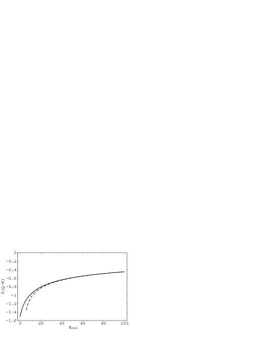
FIG. 1.: Curves for $S(Q{-}E)$ — the correction to the closure part of the sudden approximation — as a function of the energy threshold of the final ionic state, $E_{\rm max}=K^{2}/2m=Q+E_{i}-E$ and its asymptotic behavior for large $Q{-}E$. The solid curve is the plot of numerical result of $S(Q{-}E)$, the lower and dashed curve is the high energy asymptotic behavior given in Eq. (113). The units are ${\rm R\!y}^{2}$ for the vertical axis and ${\rm R\!y}$ for the horizontal axis.

FIG. 2.: Curves for $P_{1}(Q-E)$ — a function measuring the change of the spectrum due to per unit change of the neutrino mass squared — as a function of the energy threshold of the final ionic state, $E_{\rm max}=K^{2}/2m=Q+E_{i}-E$ and its asymptotic behavior for large $Q{-}E$. The solid curve is the plot of numerical result of $P_{1}(Q-E)$, the lower and dashed curve is the high energy asymptotic behavior given in Eq. (114). The units are $1$ for the vertical axis and ${\rm R\!y}$ for the horizontal axis.

B ${\tilde{K}}_{fi}$ Corrections

In this section, we shall deal with the contribution to the inclusive differential decay rate involving ${\tilde{K}}_{fi}$. Recalling the differential decay rate formula (95), the sums which we need to consider involve the combination $|T_{fi}|^{2}{\tilde{K}}_{fi}$. Therefore, it is convenient to define

$$K(\epsilon)\equiv\langle i|\,r^{-\epsilon}|f\rangle\langle f|\,r^{\epsilon}|i\rangle\,,$$ (115)

which is related to ${\tilde{K}}_{fi}$ via

$$|T_{fi}|^{2}\,{\tilde{K}}_{fi}={1\over 4}\,K^{\prime\prime}(0)\,,$$ (116)

in view of Eq. (86). Correspondingly, the sum

$$K_{n}(\epsilon)\equiv\sum_{f<f_{\rm max}}\;\langle i|\,r^{-\epsilon}|f\rangle\langle f|\,r^{\epsilon}|i\rangle\,(E_{i}-E_{f})^{n}\,,$$ (117)

can produce the desired sums through

$$\sum_{f<f_{\rm max}}\,|T_{fi}|^{2}\,{\tilde{K}}_{fi}\,(E_{i}-E_{f})^{n}={1\over 4}\,K_{n}^{\prime\prime}(0)\,.$$ (118)

Since the spectrum is corrected by the combination $\sum_{f<f_{\rm max}}|T_{fi}|^{2}{\tilde{K}}_{fi}(Q_{f}-E)^{2}$, in view of the relation (118), the contribution to the spectrum due to ${\tilde{K}}_{fi}$ can be expressed in terms of the quantity $C(Q{-}E)$ defined by

$$C(Q{-}E)\equiv(Q-E)^{2}K_{0}^{\prime\prime}(0)+2(Q-E)K_{1}^{\prime\prime}(0)+K_{2}^{\prime\prime}(0)\,.$$ (119)

The goal of this section is to show the main steps of calculating $C(Q{-}E)$ and display the numerical results of $C(Q{-}E)$.

For $n=0$, the completeness relation

$$K_{0}(\epsilon)=1-\int_{k>K}{(d^{3}{\bf k})\over(2\pi)^{3}}K(\epsilon)$$ (120)

and the $\epsilon$ derivatives give

$$K_{0}^{\prime\prime}(0)=-\int_{k>K}{(d^{3}{\bf k})\over(2\pi)^{3}}K^{\prime\prime}(0)=-{1\over 2\pi^{2}a_{0}^{3}}\int_{0}^{1/(Ka_{0})}d\gamma\,\gamma^{-4}K^{\prime\prime}(0)\,.$$ (121)

With this, $K_{0}$ may be then directly evaluated by exploiting the numerical results for $K^{\prime\prime}(0)$ obtained in Appendix C.

For $n=1$, we may write similarly

$$K_{1}(\epsilon)=\langle i|(H_{i}r^{\epsilon}-r^{\epsilon}H_{f})r^{-\epsilon}|i\rangle-\int_{k>K}{(d^{3}{\bf k})\over(2\pi)^{3}}K(\epsilon)\left(E_{i}-E_{k}\right)\,.$$ (122)

The first, closure-approximation term is readily evaluated:

$$\langle i|(H_{i}r^{\epsilon}-r^{\epsilon}H_{f})r^{-\epsilon}|i\rangle = \langle i|\left[{e^{2}\over 4\pi r}+{\epsilon^{2}\over 2mr^{2}}+{i\epsilon\over 2m}\left({\bf p}\cdot{{\bf r}\over r^{2}}+{{\bf r}\over r^{2}}\cdot{\bf p}\right)\right]|i\rangle$$ (123)

$$= 2(1+\epsilon^{2}){\rm R\!y}\,.$$ (124)

Therefore,

$$K_{1}^{\prime\prime}(0) = \left[4+\int_{k>K}{(d^{3}{\bf k})\over(2\pi)^{3}}K^{\prime\prime}(0)(1+\gamma^{-2})\right]{\rm R\!y}$$ (125)

$$= \left[4+{1\over 2\pi^{2}a_{0}^{3}}\int_{0}^{1/(Ka_{0})}d\gamma\gamma^{-6}(1+\gamma^{2})\,K^{\prime\prime}(0)\right]{\rm R\!y}\,,$$ (126)

which enables again a simple numerical calculation of $K_{1}^{\prime\prime}(0)$ upon using the result of $K^{\prime\prime}(0)$.

For the case $n=2$, since the closure approximation result diverges, we shall use a different formalism. It is convenient to separate the sum in the definition (117), and thus the definition for $K_{2}^{\prime\prime}(0)$, into two parts: the contribution from summing the final ionic bound states denoted by

$$K_{\rm 2b}=\sum_{b}K^{\prime\prime}(0)(E_{i}-E_{f})^{2}\,,$$ (127)

and the contribution from the continuum with energy under the threshold $K^{2}/2m$ denoted by

$$K_{\rm 2c}=\int_{k<K}{(d^{3}{\bf k})\over(2\pi)^{3}}K^{\prime\prime}(0)(E_{i}-E_{k})^{2}={1\over 2\pi^{2}}\int_{1/Ka_{0}}^{\infty}d\gamma\,\gamma^{-8}(1+\gamma^{2})\,K^{\prime\prime}(0)\,{\rm R\!y}^{2}\,.$$ (128)

The sum of $K_{\rm 2b}$ and $K_{\rm 2c}$ produces $K_{2}^{\prime\prime}(0)$. The second part $K_{\rm 2c}$ can again be readily evaluated by using the numerical results for $K^{\prime\prime}(0)$ given in Appendix C, and this Appendix also provides the evaluation

$$K_{\rm 2b}=32.26\,{\rm R\!y}^{2}\,.$$ (129)

The curve for $C(Q{-}E)$ as a function of the threshold energy $E_{\rm max}$ is shown in Fig. 3.

FIG. 3.: Curve for $C(Q{-}E)$ — the correction to the spectrum due to ${\tilde{K}}_{fi}$ as a function of the threshold energy of the final ionic state $E_{\rm max}=K^{2}/2m=Q+E_{i}-E$; the units are ${\rm R\!y}^{2}$ for the vertical axis and ${\rm R\!y}$ for the horizontal axis.

We find that a quadratic function $C_{f1}(Q{-}E)$,

$$C_{f1}(Q{-}E) = 33.6\,{\rm R\!y}^{2}+4.92\,{\rm R\!y}\,E_{\rm max}+0.0148\,E_{\rm max}^{2}$$ (130)

$$= 28.7\,{\rm R\!y}^{2}+4.89\,{\rm R\!y}\,(Q-E)+0.0148\,(Q-E)^{2}\,,$$ (131)

describes $C(Q{-}E)$ for $E_{\rm max}$ in the range $0-64\,{\rm R\!y}$ ($0-870$ eV) with a good accuracy. To analyze how the atomic effects change the experimental data fitting, we fit $C(Q{-}E)$ to a linear combination of the functions $P(Q{-}E)$, $P^{\prime}(Q{-}E)$, and $P_{1}(Q{-}E)$ in the same range of the spectrum and get

$$C(Q{-}E)\approx C_{f2}(Q{-}E)\equiv 0.0148\,P(Q{-}E)+2.42\,{\rm R\!y}\,P^{\prime}(Q{-}E)+18.9\,{\rm R\!y}^{2}P_{1}(Q{-}E)\,.$$ (132)

We show $C(Q{-}E)$ and its two fitting formula $C_{f1}(Q{-}E)$ and $C_{f2}(Q{-}E)$ simultaneously in Fig. 4. The three curves can barely be distinguished. The errors due to the fitting are shown in Fig. 5 for $C_{f1}(Q{-}E)$ and Fig. 6 for $C_{f2}(Q{-}E)$ respectively.

FIG. 4.: Curves for $C(Q{-}E)$ and its two fitting forms $C_{f1}(Q{-}E)$ and $C_{f2}(Q{-}E)$ which can barely be distinguished. The units are the same as in previous figure, ${\rm R\!y}^{2}$ for the vertical axis and ${\rm R\!y}$ for the horizontal axis.

FIG. 5.: Curve for the difference $C_{f1}(Q{-}E)-C(Q{-}E)$ as a function of $E_{\rm max}=Q+E_{i}-E$. The units are the same as in previous figure, ${\rm R\!y}^{2}$ for the vertical axis and ${\rm R\!y}$ for the horizontal axis.

FIG. 6.: Curve for the difference $C_{f2}(Q{-}E)-C(Q{-}E)$ as a function of $E_{\rm max}=Q+E_{i}-E$. The units are the same as in previous figure, ${\rm R\!y}^{2}$ for the vertical axis and ${\rm R\!y}$ for the horizontal axis.

V Final atomic states with non-zero angular momentum

So far, we have considered only the final ion state $\langle f|$ being in an S-state. To obtain the inclusive decay rate, we also need to consider the case where the final ion states are not S-states. For these cases, the first term $T_{1}$, the amplitude of the sudden approximation, vanishes. Therefore, to order $\eta^{2}$, as far as the decay rate is concerned, it is sufficient to calculate the amplitude to order $\eta$, which comes from the leading term of $T_{\rm d}$. Recalling expression (73) for this leading term $T_{\rm d}^{0}$, we have, to order $\eta$,

$$T_{\rm d}^{0}\simeq{-}\langle{\bf p}|\!\int(d^{3}{\bf r}_{2})\phi_{f}^{*}({\bf r}_{2})\phi_{i}({\bf r}_{2})\!\left[{e^{2}\over 4\pi|{\bf r}_{1}{-}{\bf r}_{2}|}{-}{2e^{2}\over 4\pi r_{1}}{-}v(r_{1})\right]\!{1\over H_{1}{+}E_{i}{-}E{-}E_{f}{-}i\epsilon}|{\bf r}_{1}{=}{\bf 0}\rangle\,.$$ (133)

The last two terms in the square brackets vanish upon integrating over the solid angle of ${\bf r}_{2}$ since now $\phi_{f}({\bf r}_{2})$ contains only higher partial waves with $l\geq 1$. Hence

$$T_{\rm d}^{0}\simeq-\int(d^{3}{\bf r}_{2})\phi_{f}^{*}({\bf r}_{2})\phi_{i}({\bf r}_{2})\langle{\bf p}|{e^{2}\over 4\pi|{\bf r}_{1}-{\bf r}_{2}|}{1\over H_{0}-E-i\epsilon}|{\bf 0}\rangle\,,$$ (134)

where we have neglected $E_{i}$, $E_{f}$ compared with $E$ and replaced $H_{1}$ by the free Hamiltonian $H_{0}$. Suppose that final state $\langle f|$ has the angular momentum quantum number $(l,m)$, or equivalently

$$\phi_{f}^{*}({\bf r})=R_{fl}^{*}(r)Y_{lm}^{*}({\hat{\bf r}})\,,$$ (135)

with $R_{fl}(r)$ the radial wave function. In Appendix B, we find that, to the leading order,

$$T_{\rm d}^{0}\simeq i{4\pi\over l(l+1)}\eta Y_{lm}^{*}({\hat{\bf p}})\int_{0}^{\infty}dr_{2}r_{2}^{2}R_{fl}^{*}(r_{2})\phi_{i}(r_{2})\,.$$ (136)

The differential decay rate involves the angular average of the square of the spherical harmonic function which appears in Eq. (136),

$$\int{d\Omega_{\bf p}\over 4\pi}\left|Y_{lm}({\hat{\bf p}})\right|^{2}={1\over 4\pi}\,,$$ (137)

and thus, in view of Eq. (61), the differential decay rate to states with specific energy and angular momentum $l$ is given by

$${d\Gamma_{fl}\over dE}={m\over 2\pi^{3}}p\,|T_{\beta}|^{2}(Q_{f}-E)^{2}\,\eta^{2}\,{4\pi(2l+1)\over l^{2}(l+1)^{2}}\left|\int_{0}^{\infty}dr_{2}r_{2}^{2}R_{fl}^{*}(r_{2})\phi_{i}(r_{2})\right|^{2}\,,$$ (138)

where we have done the summation over the magnetic quantum number $m$ which generates the factor $2l+1$.

Summing over $l$ and $f$ produces the differential decay rate for the final ${}^{3}{\rm He}^{+}$ ion having nonzero angular momentum. Using the expansion (96) we encounter the sums

$$M_{n}=\sum_{fl}{4\pi(2l+1)\over l^{2}(l+1)^{2}}\left|\int_{0}^{\infty}dr\,r^{2}R_{fl}^{*}(r)\phi_{i}(r)\right|^{2}(E_{i}-E_{f})^{n}\,,$$ (139)

with $n=0,1,2$. To facilitate the calculation, we define

$$M(k)=\left(E_{i}-E_{k}\right)^{2}\sum_{l=1}^{\infty}{4\pi(2l+1)\over l^{2}(l+1)^{2}}\left|\int_{0}^{\infty}dr\,r^{2}R_{kl}^{*}(r)\phi_{i}(r)\right|^{2}\,,$$ (140)

where $R_{kl}(r)$ is the radial wave function of the final unbound ion state with energy $E_{k}=k^{2}/(2m)$ and angular momentum $l$. $M(k)$ is calculated in Appendix C. We can consequently calculate $M_{n}$ for $n=0,1,2$.

For $n=0$, exploiting the completeness relation

$$\sum_{f}R_{fl}^{*}(r^{\prime})\,R_{fl}(r)={1\over r^{2}}\,\delta(r^{\prime}-r)\,,$$ (141)

we can write

$$M_{0} = \sum_{l}{2l{+}1\over l^{2}(l{+}1)^{2}}\int_{0}^{\infty}4\pi r^{2}dr|\phi_{i}(r)|^{2}-\sum_{l}{4\pi(2l{+}1)\over l^{2}(l{+}1)^{2}}\int_{K}^{\infty}dk{2k^{2}\over\pi}\left|\int_{0}^{\infty}dr\,r^{2}R_{kl}(r)\phi_{i}(r)\right|^{2}$$ (142)

$$= 1-\int_{K}^{\infty}dk{2k^{2}\over\pi}M(k)\left(E_{i}-E_{k}\right)^{-2}\,,$$ (143)

where the sum

$$\sum_{l=1}^{\infty}{2l+1\over l^{2}(l+1)^{2}}=\sum_{l=1}^{\infty}\left[{1\over l^{2}}-{1\over(l+1)^{2}}\right]=1$$ (144)

and the unit norm of the initial wave function $\phi_{i}(r)$ have been used. This expression enables a numerical evaluation of $M_{0}$.

To calculate $M_{1}$ and $M_{2}$, we write $M_{n}$ as the sum of two parts — $M_{n{\rm b}}$ the part coming from summing over the final bound ionic states and $M_{n{\rm c}}$ the part coming from summing over the final continuous ionic states,

$$M_{n}=M_{n{\rm b}}+M_{n{\rm c}}\,.$$ (145)

Following the definition of $M_{n{\rm c}}$, we have

$$M_{n{\rm c}}=\int_{0}^{K}dk{2k^{2}\over\pi}M(k)(E_{i}-E_{k})^{n-2}\,,$$ (146)

which may be easily calculated numerically. For $M_{n{\rm b}}$, we shall not investigate it numerically; instead, we estimate it to a good accuracy. To facilitate the notation, we define $L(Q{-}E)$ by

$$L(Q{-}E)\equiv M_{0}\,\,(Q-E)^{2}+2M_{\rm 1c}\,\,(Q-E)+M_{\rm 2c}\,,$$ (147)

which enables us to write the differential inclusive decay rate for the final ion state having nonzero angular momentum as

$${d\Gamma^{\prime}\over dE}\equiv\sum_{fl}{d\Gamma_{fl}\over dE}={m\over 2\pi^{3}}\,p\,|T_{\beta}|^{2}\,\eta^{2}\,\left[L(Q{-}E){+}2M_{\rm 1b}(Q{-}E){+}M_{\rm 2b}\right]\,.$$ (148)

Upon using the numerical result of $M(k)$ obtained in Appendix C, one may obtain $M_{0}$, $M_{\rm 1c}$, and $M_{\rm 2c}$ by numerically performing the integrals over $k$ in expressions (143) and (146). Definition (147) thus gives a numerical result for $L(Q{-}E)$ which we display as a function of $E_{\rm max}=K^{2}/(2m)$ in Fig. 7. We find also a quadratic function $L_{f1}(Q{-}E)$

$$L_{f1}(Q{-}E) = 5.90\,{\rm R\!y}^{2}-1.03\,{\rm R\!y}\,E_{\rm max}+0.947\,E_{\rm max}^{2}$$ (149)

$$= 7.88\,{\rm R\!y}^{2}-2.93\,{\rm R\!y}\,(Q-E)-0.947\,(Q-E)^{2}$$ (150)

which fits $L(Q{-}E)$ for $E_{\rm max}$ in the range $0-64\,{\rm R\!y}$ ($0-870$ eV) with a fairly good accuracy. Like in previous section, we fit $L(Q{-}E)$ to a linear combination of functions $P(Q{-}E)$, $P^{\prime}(Q{-}E)$, and $P_{1}(Q{-}E)$ to generate the fitting formula

$$L(Q{-}E)\approx L_{f2}(Q{-}E)\equiv 0.948P(Q{-}E)-3.39{\rm R\!y}P^{\prime}(Q{-}E)+15.7{\rm R\!y}^{2}P_{1}(Q{-}E)\,.$$ (151)

We show $L(Q{-}E)$ and its two fitting functions $L_{f1}(Q{-}E)$ and $L_{f2}(Q{-}E)$ together in Fig. 8. They can hardly be distinguished. The errors caused by the fitting are shown in Fig. 9 for $L_{f1}(Q{-}E)$ and Fig. 10 for $L_{f2}(Q{-}E)$ respectively.

FIG. 7.: Numerical curve for $L(Q{-}E)$ — the correction to the spectrum due to atomic effect for non-S-wave final ionic states — as a function of $E_{\rm max}=Q+E_{i}-E$; vertical axis has the unit ${\rm R\!y}^{2}$ and horizontal axis has the unit ${\rm R\!y}$.

FIG. 8.: Numerical curve for $L(Q{-}E)$ and its two fitting formula $L_{f1}(Q{-}E)$ and $L_{f2}(Q{-}E)$ as functions of $E_{\rm max}=Q+E_{i}-E$; vertical axis has the unit ${\rm R\!y}^{2}a_{0}^{3}$ and horizontal axis has the unit ${\rm R\!y}$.

FIG. 9.: Numerical curve for the difference between $L_{f1}(Q{-}E)-L(Q{-}E)$ as a function of $E_{\rm max}=Q+E_{i}-E$, vertical axis has the unit ${\rm R\!y}^{2}$ and horizontal axis has the unit ${\rm R\!y}$.

FIG. 10.: Numerical curve for the difference between $L_{f2}(Q{-}E)-L(Q{-}E)$ as a function of $E_{\rm max}=Q+E_{i}-E$, vertical axis has the unit ${\rm R\!y}^{2}$ and horizontal axis has the unit ${\rm R\!y}$.

We now turn to provide numerical bounds for $M_{\rm 1b}$ and $M_{\rm 2b}$. The energy of an ionic state with principal quantum number $n_{f}$ is given by

$$E_{f}={4\over n_{f}^{2}}E_{i}=-{4\over n_{f}^{2}}{\rm R\!y}\,.$$ (152)

Since the lowest energy state with nonzero angular momentum ($n_{f}=2$) has the energy $E_{i}$, it does not contribute to the summation defining $M_{n{\rm b}}$ for $n=1,2$ due to the factor $(E_{i}-E_{f})^{n}$. For the other states, since $n_{f}>2$, $E_{f}\geq 4E_{i}/9$, and hence

$$(E_{f}-E_{i})^{n}\geq\left({5\over 9}\,{\rm R\!y}\right)^{n}\,.$$ (153)

Therefore, according the definition of $M_{n{\rm b}}$, we have

$$-M^{\prime}_{\rm 0b}\,\,{5\over 9}\,\,{\rm R\!y}> M_{\rm 1b} >-M^{\prime}_{\rm 0b}\,\,{\rm R\!y}\,,$$ (154)

$$M^{\prime}_{\rm 0b}\,\,{25\over 81}\,\,{\rm R\!y}^{2}< M_{\rm 2b} <M^{\prime}_{\rm 0b}\,\,{\rm R\!y}^{2}\,,$$ (155)

where $M^{\prime}_{\rm 0b}$ is defined by excluding the lowest energy state ($n_{f}{=}2,l{=}1$) in the $(n_{f},l)$ summation of the definition of $M_{\rm 0b}$, i.e.,

$$M^{\prime}_{\rm 0b}\equiv M_{\rm 0b}-{3\over 4}\,4\pi\left|\int_{0}^{\infty}drr^{2}R_{21}(r)\phi_{i}(r)\right|^{2}\,.$$ (156)

Evaluating the matrix element,

$$4\pi\left|\int_{0}^{\infty}drr^{2}R_{21}(r)\phi_{i}(r)\right|^{2}={3\over 4}\,,$$ (157)

and using the numerical result

$$M_{\rm 0b}=0.659\,,$$ (158)

gives the explicit bounds:

$$-0.05\,{\rm R\!y}>M_{\rm 1b}>-0.1\,{\rm R\!y}\,,\qquad 0.03\,{\rm R\!y}^{2}<M_{\rm 2b}<0.1\,{\rm R\!y}^{2}\,.$$ (159)

VI Inclusive Decay Rate

Adding the differential decay rates (97) and (148), we find that the inclusive differential decay rate is given by

$${d\Gamma_{\rm in}\over dE} = {d\Gamma_{0}\over dE}+{d\Gamma^{\prime}\over dE}$$ (160)

$$\simeq {m\over 2\pi^{3}}F(2,E)\,p\,|T_{\beta}|^{2}(1{-}2\eta^{2})\left[P(Q-E)+\eta^{2}R(Q{-}E)]\right]\,,$$ (161)

where we have defined the correction term $R(Q{-}E)$ by

$$R(Q{-}E)\equiv-{C(Q{-}E)\over 2}+L(Q{-}E)+2M_{\rm 1b}(Q-E)+M_{\rm 2b}\,,$$ (162)

and dropped higher order terms. Here $C(Q{-}E)$ and $L(Q{-}E)$ are evaluated numerically; $M_{\rm 1b}$ and $M_{\rm 2b}$ are very small contributions bounded by Eq. (159). The term containing $R(Q{-}E)$ in the second line of Eq. (161) represents the correction to the sudden approximation result due to the atomic effect.

A Comparing with previous results

We now compare our result (161) with previous results [11, 12]. To reproduce the previous results, two approximations must be made, as mentioned in Section I. Under the “uniform phase space factor approximation”, we have

$$C(Q{-}E)\sim(Q-{\bar{E}})^{2}K_{0}^{\prime\prime}(0)\,,$$ (163)

$$L(Q{-}E)\sim(Q-{\bar{E}})^{2}M_{0}\,,$$ (164)

where ${\bar{E}}$ is some average beta ray energy which differs from the beta ray energy $E$ by an amount of order ${\rm R\!y}$. Under the closure approximation, Eq. (121) and Eq. (143) read $K_{0}^{\prime\prime}(0)\simeq 0$ and $M_{0}\simeq 1$ respectively. With these approximations, the definition (162) gives $R(Q{-}E)\sim(Q-{\bar{E}})^{2}$, which implies that the result (161) above reduces to a modified sudden approximation result:

$${d\Gamma_{\rm in}\over dE}={m\over 2\pi^{3}}F(2,E){p^{\prime}}\,|T_{\beta}|^{2}P(Q-E)\,,$$ (165)

where terms of order $\eta^{2}S(Q{-}E)$ and $\eta^{2}{\rm R\!y}^{2}$ have been discarded with the approximations we are considering. The result (165) agrees with previous results [11, 12], with the modified momentum ${p^{\prime}}$ being defined by

$${{p^{\prime}}^{2}\over 2m}+2\,{\rm R\!y}={p^{2}\over 2m}\,.$$ (166)

The momentum ${p^{\prime}}$ equals the momentum of an emitted beta electron whose energy at short distances is modified by the repulsive Coulomb interaction energy with the original electron bound in the tritium atom. This modification which changes $p$ to ${p^{\prime}}$ was found by Rose a long time ago [13].

B Estimation of the atomic effects in the neutrino mass determination

To estimate how the atomic effects change the neutrino mass squared parameter, we first recall that the spectrum used in the experimental data analysis is the sudden approximation result [2, 3, 4, 5, 6, 7]

$${d\Gamma_{\rm exp}\over dE}=A\,\,F(2,E)\,\,p\sum_{f<f_{\rm max}}W_{fi}(Q_{f}-E)\,\sqrt{(Q_{f}-E)^{2}-m_{\nu}^{2}}\,.$$ (167)

The terms in the right hand side of Eq. (167) require some explanation. The first factor $F(2,E)$ is the usual Fermi function with the nucleus charge $Z=2$, and $p$ is the momentum of the beta ray. $W_{fi}$ is the transition probability for the initial tritium state decaying to the state $f$ of the final ${}^{3}{\rm He}^{+}$ ion. In real experiments, molecular tritium is used. Therefore, $W_{fi}$ is the square of the matrix element for the molecular state. Since only atomic tritium is considered in this article, we have made the replacement $W_{fi}=|T_{fi}|^{2}$. Finally, $m_{\nu}^{2}$ is the neutrino mass squared. Though one focuses on measuring the beta ray spectrum near the end point to probe the neutrino mass, most of the data obtained in the experiments are in the range where $(E-Q)^{2}\gg m_{\nu}^{2}$ since the decay rate is tiny at the very end of the spectrum. Expanding the square root, we get

$${d\,\Gamma_{\rm exp}\over dE} \simeq A\,\,F(2,E)\,\,p\sum_{f<f_{\rm max}}|T_{fi}|^{2}\left[(Q_{f}-E)^{2}-{1\over 2}m_{\nu}^{2}\right]$$ (168)

$$= A\,\,F(2,E)\,\,p\,\left[P(Q{-}E)-{1\over 2}m_{\nu}^{2}P_{1}(Q{-}E)\right]\,,$$ (169)

where we have used the definitions (11) and (14) for the functions $P(Q{-}E)$ and $P_{1}(Q{-}E)$ which are evaluated numerically in section IV.

In real experimental data analysis, the parameters $A$, $Q$, and $m_{\nu}^{2}$ are determined by comparing the spectrum (169) with the measured spectrum. Therefore, any theoretical correction to the spectrum (169) has the effect of changing the parameters $A\to{\bar{A}}=A+\Delta A$, $Q\to{\bar{Q}}=Q+\Delta Q$, and $m_{\nu}^{2}\to\Delta m_{\nu}^{2}$ so that the theoretical correction to the spectrum may be included by using an effective spectrum described by the same form (169) but with the effective parameters ${\bar{A}}$, ${\bar{Q}}$, and $\Delta m_{\nu}^{2}$. The change of the spectrum (169)

$$\Delta\left({d\Gamma_{\rm exp}\over dE}\right)\approx A\,\,F(2,E)\,\,p\left[{\Delta A\over A}\,P(Q{-}E)+\Delta QP^{\prime}(Q{-}E)-{1\over 2}\Delta m_{\nu}^{2}P_{1}(Q{-}E)\right]$$ (170)

mimics the corresponding theoretical correction to the spectrum.

We now estimate $\Delta Q$, $\Delta m_{\nu}^{2}$ corresponding to the correction due to the atomic effect which accounts for the interaction between the beta ray and the electron of the ${}^{3}{\rm He}^{+}$ ion. This we shall do by requiring the correction $R(Q{-}E)$ in Eq. (161) be mimicked by a linear combination of $P(Q{-}E)$, $P^{\prime}(Q{-}E)$, and $P_{1}(Q{-}E)$ as appearing in the right hand side of Eq. (170). We can neglect the small parameters $M_{\rm 1b}$ and $M_{\rm 2b}$ since they are bound by Eq. (159). Since the region important for the neutrino mass measurement goes from the the beta ray end point to approximately $59-74\,{\rm R\!y}$ ($800-1000\,{\rm eV}$) below end point[2, 3, 4, 5, 6], the previous fitting formula $C_{f2}(Q{-}E)$ and $L_{f2}(Q{-}E)$ for the energy $E_{\rm max}$ range $0-64{\rm R\!y}$ may be used here. We shall discuss the sensitivity to the range of the energy of the result later. Replacing $C(Q{-}E)$ and $L(Q{-}E)$ with their fitting formulas (132) and (151), the definition (162) reads

$$R(Q{-}E)\approx 0.94\,P(Q{-}E)-4.6\,{\rm R\!y}\,P^{\prime}(Q{-}E)+6.3\,{\rm R\!y}^{2}\,P_{1}(Q{-}E)\,.$$ (171)

Inserting this fitting form of $R(Q{-}E)$ into Eq. (161) yields

$${d\Gamma_{\rm in}\over dE} \approx {m\over 2\pi^{3}}F(2,E)p\,|T_{\beta}|^{2}(1{-}1.06\,\eta^{2})$$ (173)

$$\qquad\times\left[P(Q{-}E)-4.6\,\eta^{2}\,{\rm R\!y}\,P^{\prime}(Q{-}E)+6.3\,\eta^{2}\,{\rm R\!y}^{2}\,P_{1}(Q{-}E)\right]\,,$$

where we have shifted the argument of $P$ to absorb the second term which causes an negligible error of order $O(\eta^{4})$. In view of the argument above, specifically Eq. (170), Eq. (173) shows that the atomic effect gives a correction to neutrino mass squared of

$$\Delta m_{\nu}^{2}\approx-12.6\,\eta^{2}{\rm R\!y}^{2}\simeq-1.7\,{\rm eV}^{2}\,,$$ (174)

and the endpoint changes by

$$\Delta Q\approx-4.6\,\eta^{2}{\rm R\!y}\simeq-0.047\,{\rm eV}\,.$$ (175)

We now examine the sensitivity of the result to the energy range $E_{\rm max}$ used in the fit. Since $\Delta Q$ is tiny, we shall only consider how $\Delta m_{\nu}^{2}$ depends on the range in which we do the fit. We fit $R(Q{-}E)$ in various energy $E_{\rm max}$ ranges and display the corresponding $m_{\nu}^{2}$ in Table I shown in the introduction. The neutrino mass squared has basically a linear dependence on the energy range where we do the fit. Increasing the energy range by each $5\,{\rm R\!y}$ causes $\Delta m_{\nu}^{2}$ to decrease by $-0.4\,{\rm eV}^{2}$. The atomic effect changes the neutrino mass squared parameter on the order of a few ${\rm eV}^{2}$. It is not a big effect.

VII Conclusion

We have developed a systematic expansion for the tritium beta decay amplitude in the Coulomb parameter $\eta$. By choosing a convenient comparison potential, one can avoid the infrared divergences due to the long range characteristic of the Coulomb force. Both the exclusive and the inclusive decaying rates are calculated to order $\eta^{2}$. The inclusive decay rate agrees with previous results. The estimation on how this order $\eta^{2}$ correction affects the neutrino mass squared parameter is provided. We find that the effect is small and does not suffice to explain the mysterious negative electron anti-neutrino mass squared obtained in modern experimental data analysis[1, 2, 3, 4, 5, 6]. We also remark that the order $\eta^{2}$ correction to the spectrum is small and can not provide any explanation for the anomalous structure in the beta decay spectrum in the last 55 eV closest to the end point presented in the last article of reference[5].

A Wave function calculation

We shall find the value of the wave function $\phi_{\bf p}^{*}({\bf r})$ at the origin up to and including terms of order $\eta^{3}$. Since $\phi_{\bf p}^{*}(0)$ involves only the S-wave component, we may replace

$$\phi_{\bf p}({\bf r})\to{1\over pr}u_{p}(r)\,,$$ (A1)

where $u_{p}(r)$ obeys the S-wave radial Schrödinger equation

$$\left\{-{1\over 2m}{d^{2}\over dr^{2}}+v(r)-E\right\}u_{p}(r)=0\,.$$ (A2)

The radial wave function $u_{p}(r)$ vanishes at the origin and obeys the asymptotic boundary condition

$$r\to\infty:\quad u_{p}(r)\sim{1\over 2i}\left[e^{ipr+i\eta\ln(2pr)}-e^{-ipr-i\eta\ln(2pr)-2i\delta_{0}}\right]\,,$$ (A3)

where $\delta_{0}$ is the S-wave phase shift. This boundary condition contains a non-trivial phase structure because, at large distances, the particle moves in the long-range Coulomb field of unit charge.

It is convenient to divide space into two regions: $0<r<r_{c}$ and $r_{c}<r<\infty$, with $r_{c}$ being an intermediate distance between the Bohr radius $a_{0}$ and the de Broglie wave length $1/p=\eta a_{0}$. We take $r_{c}$ to be of the order

$$\left({r_{c}/a_{0}}\right)^{2}\sim O(\eta^{1+\zeta})\,,$$ (A4)

with $0<\zeta<1$ (e. g. $r_{c}=\eta^{2/3}a_{0}$). As we shall see, there are two reasons for this choice. One reason is that in the region where $0<r<r_{c}$, we have $r\ll a_{0}$ which enables us to expand the expression (74) for $v(r)$ as

$$v(r)=-{2e^{2}\over 4\pi r}+V_{fi}+O(e^{2}\eta^{3}p^{3}r^{2})\,,$$ (A5)

where

$$V_{fi}=\lim_{r\to 0}\left[v(r)+{2e^{2}\over 4\pi r}\right]=\int(d^{3}{\bf r})\rho_{fi}(r){e^{2}\over 4\pi r}\,.$$ (A6)

The expansion (A5) of $\Delta v(r)$ does not contain a term linear in $r$. Such a term would correspond to a charge distribution $-\nabla^{2}r\sim 1/r$ which has an unphysical singularity at the origin. The correction to the first two terms in the expansion (A5) comes from the consideration that, for any reasonable comparison potential, the characteristic length scale for $\Delta v(r)$ to vary is the Bohr radius $a_{0}$, and so the leading correction is of the order

$${e^{2}\over r}\left({r\over a_{0}}\right)^{3}\sim e^{2}\eta^{3}p^{3}r^{2}\,.$$ (A7)

Inserting the expansion (A5) of the potential into the radial Schrödinger equation (A2), we see that the “interior” solution $u_{p}(r)$ in the region $0<r<r_{c}$ is a constant $C$ times the Coulomb S-state radial wave function with charge $2$ and energy $E_{p^{\prime}}=E-V_{fi}$. This radial wave function involves the shifted momentum

$$p^{\prime}=\sqrt{p^{2}-2mV_{fi}}$$ (A8)

and the correspondingly altered Coulomb parameter

$$2\eta^{\prime}=2\alpha m/p^{\prime}\,.$$ (A9)

In the region $r<r_{c}$, the higher order terms in the expansion (A5) give rise to corrections, compared with the energy $E$ of the beta ray, of order

$${e^{2}\eta^{3}p^{3}r^{2}\over E}\sim\eta^{4}(pr)^{2}\leq\eta^{4}(pr_{c})^{2}\sim o(\eta^{3})\,,$$ (A10)

for our choice (A4) of $r_{c}$. Therefore, this Coulomb wave function with the shifted momentum $p^{\prime}$ obeys the Schrödinger equation (A2) with an error which is less than order $\eta^{3}$. As is well known [16], this wave function gives the limits,

$$r\to 0:\quad u_{p}(r)\to Cp^{\prime}re^{\pi\eta^{\prime}}\Gamma(1+2i\eta^{\prime})\,,$$ (A11)

and

$$r\to\infty:\quad u_{p}(r)\sim C\left[1+{4\eta^{\prime}\over p^{\prime}r}\right]^{-1/4}{1\over 2i}{\Biggl{\{}}e^{ip^{\prime}r+2i\eta^{\prime}\ln p^{\prime}r}+\cdots{\Biggr{\}}}\,,$$ (A12)

where the ellipsis $\cdots$ stands for the incoming wave contribution which involves $\exp\{-i(p^{\prime}r+2\eta^{\prime}\ln 2p^{\prime}r)\}$. Note that, for $r\sim r_{c}$, the asymptotic expansion (A12) is valid because $pr\gg 1$ in this region. This is the other reason for the choice (A4) of $r_{c}$.

In the region where $r>r_{c}$, we can get the asymptotic form of the wave function $u_{p}(r)$ by iterating Eq. (A2) starting with the limiting behavior (A3) of $u_{p}(r)$ for $r\to\infty$. Matching this “exterior” solution with the previous “interior” solution at $r\sim r_{c}$ determines the constant $C$. The two linearly independent solutions at large radius $r$ correspond to outgoing and incoming waves,

$$u_{p}(r)=u_{p}^{(+)}(r)+u_{p}^{(-)}(r)\,.$$ (A13)

Since we have only one constant $C$ to be determined, it is sufficient to match the outgoing wave part $u_{p}^{(+)}(r)$ to connect the solutions in the two regions. We write this part of the exterior solution as the W.K.B. approximate solution times an arbitrary function,

$$u_{p}^{(+)}(r)={1\over 2i}\left[{E\over E-v(r)}\right]^{1/4}e^{iS(r)}\,w_{p}^{(+)}(r)\,.$$ (A14)

Here $S(r)$ is defined by

$${dS(r)\over dr}=\sqrt{2m[E-v(r)]}\,,$$ (A15)

with the boundary condition that

$$S(r)\to pr+\eta\ln 2pr\,,\quad{\rm as}\,r\to\infty\,,$$ (A16)

which is consistent with the long-range limit of $v(r)$ in Eq. (A15). Thus, the boundary condition (A3) is obeyed by requiring that $w_{p}^{(+)}(r)\to 1$ as $r\to\infty$. Iterating the solution (A14) in the Schrödinger equation (A2) yields the asymptotic expansion of $w_{p}^{(+)}(r)$. For example, the first iteration gives

$$w_{p}^{(+)}(r)\simeq 1-{im\over 4p^{3}}{dv(r)\over dr}\,.$$ (A17)

When $r\sim r_{c}$, which is in the asymptotic region, the form (A14) for $u_{p}^{(+)}(r)$ with $w_{p}^{(+)}(r)=1$ is appropriate for our discussion. In the region $r\sim r_{c}$, the first factor containing the power $1/4$ in the solution (A14), by using the expansion (A5), can be written as

$$\left[{E\over E-v(r)}\right]^{1/4}\simeq\sqrt{p\over p^{\prime}}\left[1+{4\eta^{\prime}\over p^{\prime}r}\right]^{-1/4}\,,$$ (A18)

which matches the corresponding factor in the asymptotic expansion (A12) of the interior solution. The phase $S(r)$, in this region, to order $\eta^{3}$, is given by

$$S(r)\approx p^{\prime}r+2\eta^{\prime}\ln 2p^{\prime}r+\Theta\,,$$ (A19)

where $\Theta$ is a constant phase. The fact that $\Theta$ is a constant may be justified by observing that

$${d\over dr}\left[S(r)-p^{\prime}r-2\eta^{\prime}\ln 2p^{\prime}r\right] = \sqrt{2m(E-v(r))}-{m^{2}v(r)^{2}\over 2p^{3}}-p^{\prime}-{2i\eta^{\prime}\over r}$$ (A20)

$$\approx p-{mv(r)\over p}-{m^{2}v(r)^{2}\over 2p^{3}}-p^{\prime}-{2i\eta^{\prime}\over r}=o({\eta^{3}\over r_{c}})\,,$$ (A21)

where we have used the definition of $S(r)$, expanded the square root in powers of $v(r)$, and replaced $v(r)$ by its expansion (A5). Therefore, in the region where $r\sim r_{c}$, the leading terms in the solutions (A14) and (A12) match to the order $\eta^{3}$. We did not include, in the asymptotic expansions (A12) and (A14), sub-leading terms in $1/r$ such as $\eta/(pr)^{2}$ and $\eta/(pr)^{3}$ which are of the order $O(\eta^{2})$ and $O(\eta^{3})$ in the matching region. These terms must also match to the order $\eta^{3}$ because we are solving the same differential equation by using different approaches with both having an accuracy of order $\eta^{3}$. For example, the first correction in Eq. (A17) shows the matching of terms of order $\eta/(pr)^{2}$, if we recall the leading behavior of $v(r)$ at the region $r\sim r_{c}$ and include the term of order $\eta/(pr)^{2}$ in the asymptotic behavior (A12).

Requiring that the outgoing wave in the asymptotic form (A12) to be the same as that of $u_{p}^{(+)}(r)$ in Eq. (A14) thus gives

$$C\simeq\sqrt{{p\over p^{\prime}}}\,e^{i\Theta}\,.$$ (A22)

Consequently, inserting this expression for $C$ into Eq. (A11) and using Eq. (A1) gives, including terms up to order $\eta^{3}$,

$$\phi_{\bf p}(0)=e^{\pi\eta^{\prime}}\Gamma(1+2i\eta^{\prime})\sqrt{{p^{\prime}\over p}}\,e^{i\Theta}\,.$$ (A23)

The phase $\Theta$ is, of course, irrelevant since only the absolute value of the reduced matrix element occurs in the decay rate.

B Second Order Corrections

1 Evaluation of $J_{fi}$

We now calculate $J_{fi}$ defined by Eq. (84). Defining

$$L_{\bf p}({\bf r})\equiv\langle{\bf p}|\left[{1\over|{\bf r}_{1}{-}{\bf r}|}{-}{1\over r_{1}}{-}\Delta{\bar{v}}(r_{1})\right]{1\over H_{0}{-}E{-}i\epsilon}\left({1\over|{\bf r}_{1}{-}{\bf r}|}{-}{1\over r}\right){1\over H_{0}{-}E{-}i\epsilon}|{\bf r}_{1}{=}{\bf 0}\rangle$$ (B1)

with $\Delta{\bar{v}}(r)$ being given by

$${e^{2}\over 4\pi}\Delta{\bar{v}}(r)\equiv v(r)+{e^{2}\over 4\pi r}\,,$$ (B2)

expresses $J_{fi}$ as

$$\eta^{2}J_{fi}=\left({e^{2}\over 4\pi}\right)^{2}\int(d^{3}{\bf r})\rho_{fi}(r)L_{\bf p}({\bf r})\,.$$ (B3)

The representation

$${1\over H_{0}-E-i\epsilon}=i\int_{0}^{\infty}dte^{-it(H_{0}-E)}\,,$$ (B4)

expresses

$$L_{\bf p}({\bf r})=-\int_{0}^{\infty}\!dt\!\int_{0}^{\infty}\!dt^{\prime}\langle{\bf p}|\left({1\over|{\bf r}_{1}{-}{\bf r}|}{-}{1\over r_{1}}{-}\Delta{\bar{v}}(r_{1})\right)e^{-it(H_{0}{-}E)}\left({1\over|{\bf r}_{1}{-}{\bf r}|}{-}{1\over r}\right)e^{-it^{\prime}(H_{0}{-}E)}|{\bf r}_{1}{=}{\bf 0}\rangle\,.$$ (B5)

By introducing the Heisenberg picture operator

$${\bf r}_{1}(t)\equiv e^{iH_{0}t}{\bf r}_{1}e^{-iH_{0}t}\,,$$ (B6)

$L_{\bf p}({\bf r})$ may be simply expressed as

$$L_{\bf p}({\bf r}) = -\int_{0}^{\infty}dt\int_{0}^{\infty}dt^{\prime}\,\langle{\bf p}|\left({1\over|{\bf r}_{1}(t+t^{\prime})-{\bf r}|}-{1\over r_{1}(t+t^{\prime})}-\Delta{\bar{v}}[r_{1}(t{+}t^{\prime})]\right)$$ (B8)

$$\qquad\qquad\qquad\qquad\qquad\times\left({1\over|{\bf r}_{1}(t^{\prime})-{\bf r}|}-{1\over r}\right)|{\bf r}_{1}{=}{\bf 0}\rangle\,,$$

where we have used $\langle{\bf p}|\;(H_{0}-E)=0$. Since the Hamiltonian $H_{0}$ describes a free particle, the equation of motion for ${\bf r}_{1}(t)$ gives

$${\bf r}_{1}(t)={\bf r}_{1}(0)+{{\bf p}_{1}\over m}t\,.$$ (B9)

We shall need only the leading order term of $L_{\bf p}({\bf r})$ for $p$ being much larger that $1/a_{0}$. This is the term that gives the leading correction of order $\eta^{2}=1/(pa_{0})^{2}$. It is then valid to treat the momentum operator ${\bf p}_{1}$ as commuting with the coordinate operator ${\bf r}_{1}$ since $[{\bf r}_{1},{\bf p}_{1}]\sim 1\ll pa_{0}$. Thus, the leading order in $\eta$ evaluation of the matrix element in Eq. (B8) is given by its classical limit with the operator ${\bf p}_{1}$ replaced by its eigenvalue ${\bf p}$ and ${\bf r}_{1}$ set to zero and with $\langle{\bf p}|{\bf r}_{1}{=}{\bf 0}\rangle$=1:

$$L_{\bf p}({\bf r})=-\int_{0}^{\infty}dt\int_{0}^{\infty}dt^{\prime}\left\{{1\over|{{\bf p}\over m}(t{+}t^{\prime})-{\bf r}|}-{1\over{p\over m}(t{+}t^{\prime})}-\Delta{\bar{v}}\left[{p\over m}(t{+}t^{\prime})\right]\right\}\left({1\over|{{\bf p}\over m}t^{\prime}-{\bf r}|}-{1\over r}\right)\,.$$ (B10)

Performing a change of variables

$$s={mr\over p}(t+t^{\prime})\,,\qquad\lambda={t^{\prime}\over t+t^{\prime}}\,,$$ (B11)

puts this in the form

$$L_{\bf p}({\bf r})=-{m^{2}\over p^{2}}\int_{0}^{\infty}dss\int_{0}^{1}d\lambda\left({1\over|{\hat{\bf p}}s-{\hat{\bf r}}|}-{1\over s}-r\,\Delta{\bar{v}}(sr)\right)\left({1\over|{\hat{\bf p}}\lambda s-{\hat{\bf r}}|}-1\right)\,.$$ (B12)

Since only the angular average in ${\bf r}$ contributes, it is convenient to use the spherical harmonic expansion

$${1\over 4\pi|{\bf r}_{1}-{\bf r}_{2}|}=\sum_{l=0}^{\infty}\sum_{m=-l}^{l}{1\over 2l+1}{r_{<}^{l}\over r_{>}^{l+1}}\,Y_{lm}^{*}({\hat{\bf r}}_{1})\,Y_{lm}({\hat{\bf r}}_{2})$$ (B13)

to obtain

$$L_{\bf p}({\bf r}) = -{m^{2}\over p^{2}}\int_{0}^{\infty}dss\int_{0}^{1}d\lambda\left[\sum_{l=1}^{\infty}\sum_{m=-l}^{l}{4\pi\over 2l{+}1}{s_{<}^{l}\over s_{>}^{l{+}1}}Y_{lm}^{*}({\hat{\bf r}})Y_{lm}({\hat{\bf p}})+\left(1{-}{1\over s}\right)\theta(1{-}s)-\Delta{\bar{v}}(sr)\right]$$ (B15)

$$\times\left[\sum_{l^{\prime}=0}^{\infty}\sum_{m^{\prime}=l^{\prime}}^{l^{\prime}}{4\pi\over 2l^{\prime}+1}{s_{<}^{\prime\;l^{\prime}}\over s_{>}^{\prime\;l^{\prime}+1}}Y_{l^{\prime}m^{\prime}}^{*}({\hat{\bf p}})Y_{l^{\prime}m^{\prime}}({\hat{\bf r}})+\left({1\over\lambda s}-1\right)\theta(\lambda s-1)\right]\,,$$

where

$$s_{<} = {\rm min}\{s,1\},\qquad s_{>}={\rm max}\{s,1\}\,,$$ (B16)

$$s^{\prime}_{<} = {\rm min}\{\lambda s,1\},\qquad s^{\prime}_{>}={\rm max}\{\lambda s,1\}\,.$$ (B17)

The orthonormality of the spherical harmonics and the property

$${4\pi\over 2l+1}\sum_{m}Y^{*}_{lm}({\hat{\bf r}})Y_{lm}({\hat{\bf r}})=P_{l}(1)=1$$ (B18)

now yield the angular average

$$\overline{L_{\bf p}({\bf r})}=-{m^{2}\over p^{2}}\int_{0}^{\infty}dss\int_{0}^{1}d\lambda\left[\sum_{l=1}^{\infty}{1\over 2l+1}{s_{<}^{l}\over s_{>}^{l+1}}{s_{<}^{\prime\;l}\over s_{>}^{\prime\;l+1}}-r\Delta{\bar{v}}(sr)\left({1\over\lambda s}-1\right)\theta(\lambda s-1)\right]\,.$$ (B19)

For the first term in the integrand, exchanging the order of the integrals and sum, it is straight forward to evaluate

$$\int_{0}^{1}d\lambda\sum_{l=1}^{\infty}{1\over 2l+1}\int_{0}^{\infty}ds\,s{s_{<}^{l}\over s_{>}^{l+1}}{s_{<}^{\prime l}\over s_{>}^{\prime l+1}}$$ (B20)

$$\quad\qquad=\int_{0}^{1}d\lambda\sum_{l=1}^{\infty}{1\over 2l+1}\left(\int_{0}^{1}ds\,s\,s^{2l+1}\lambda^{l}+\int_{1}^{1\over\lambda}ds\,s\,\lambda^{l}+\int_{1\over\lambda}^{\infty}ds\,s{1\over s^{2l+2}\lambda^{l+1}}\right)$$ (B21)

$$\quad\qquad=\int_{0}^{1}d\lambda\sum_{l=1}^{\infty}\left({\lambda^{l-1}\over 2l}-{\lambda^{l}\over 2l+2}\right)=\int_{0}^{1}d\lambda\;{1\over 2}={1\over 2}\,.$$ (B22)

Therefore,

$$\overline{L_{\bf p}({\bf r})}=-{m^{2}\over p^{2}}\left[{1\over 2}-\int_{1}^{\infty}\!\!ds\,(\ln s-s+1)\,r\,\Delta{\bar{v}}(sr)\right]\,,$$ (B23)

where we have carried out the remaining $\lambda$ integral. The expansion (B13) gives

$$\Delta{\bar{v}}(r)=\int(d^{3}{\bf r}^{\prime})\rho_{fi}(r^{\prime})\left({1\over|{\bf r}-{\bf r}^{\prime}|}-{1\over r}\right)=\int(d^{3}{\bf r}^{\prime})\rho_{fi}(r^{\prime})\theta(r^{\prime}{-}r)\left({1\over r^{\prime}}-{1\over r}\right)\,.$$ (B24)

Inserting this expression for $\Delta{\bar{v}}(r)$ into Eq. (B23) and performing the $s$ integral produces

$$\overline{L_{\bf p}({\bf r})}=-{m^{2}\over 2p^{2}}\left\{1-\int(d^{3}{\bf r}^{\prime})\rho_{fi}(r^{\prime})\theta(r^{\prime}{-}r)\left[{r\over r^{\prime}}-2+{r^{\prime}\over r}-\ln^{2}\left({r^{\prime}\over r}\right)\right]\right\}\,.$$ (B25)

Putting this result in to Eq. (B3) gives

$$J_{fi}=-\left\{1-\int(d^{3}{\bf r})\rho_{fi}(r)\int(d^{3}{\bf r}^{\prime})\rho_{fi}(r^{\prime})\left[{r\over 2r^{\prime}}-{1\over 4}\ln^{2}\left({r^{\prime}\over r}\right)\right]\right\}\,,$$ (B26)

where the fact that the integrand is symmetric in $r$ and $r^{\prime}$ has been used to replace $\theta(r{-}r^{\prime})$ by $1/2$.

To simplify this result, we note that

$${1\over r}={4\pi\over e^{2}}(H_{i}-H_{f})$$ (B27)

to obtain

$$\langle i|{1\over r}|f\rangle\langle f|r|i\rangle = {4\pi\over e^{2}}\langle i|f\rangle(E_{i}-E_{f})\langle f|r|i\rangle$$ (B28)

$$= {4\pi\over e^{2}}\langle i|f\rangle\langle f|rH_{i}-H_{f}r|i\rangle$$ (B29)

$$= {a_{0}\over 2}\langle i|f\rangle\langle f|\left[r,{\bf p}^{2}\right]|i\rangle+\langle i|f\rangle\langle f|i\rangle$$ (B30)

$$= a_{0}\langle i|f\rangle\langle f|\left(i{\hat{\bf r}}\cdot{\bf p}+{1\over r}\right)|i\rangle+\langle i|f\rangle\langle f|i\rangle\,.$$ (B31)

Since $\langle{\bf r}|i\rangle\sim\exp\{-r/a_{0}\}$,

$$ia_{0}{\hat{\bf r}}\cdot{\bf p}|i\rangle=-|i\rangle\,,$$ (B32)

and so

$$\langle i|{1\over r}|f\rangle\langle f|r|i\rangle = \langle i|f\rangle\langle f|{a_{0}\over r}|i\rangle$$ (B33)

$$= a_{0}^{2}m|T_{fi}|^{2}V_{fi}\,,$$ (B34)

or

$$\int(d^{3}{\bf r}_{1})\rho_{fi}(r_{1})\int(d^{3}{\bf r}_{2})\rho_{fi}(r_{2})\left({r_{2}\over r_{1}}\right)=a_{0}^{2}mV_{fi}\,.$$ (B35)

Therefore, $J_{fi}$ can be repackaged as

$$J_{fi}={1\over 2}{\tilde{v}}_{fi}-1-{\tilde{K}}_{fi}\,,$$ (B36)

with

$${\tilde{K}}_{fi}={1\over 4}\int(d^{3}{\bf r}_{1})\rho_{fi}(r_{1})\int(d^{3}{\bf r}_{2})\rho_{fi}(r_{2})\ln^{2}\left({r_{2}\over r_{1}}\right)\,.$$ (B37)

This is the result (86) quoted in the text.

We shall calculate ${\tilde{K}}_{fi}$ for the final ${}^{3}{\rm He}^{+}$ state being in $1s$, $2s$, and $3s$ states. To evaluate ${\tilde{K}}_{fi}$, it is convenient to consider the integral

$$I(\epsilon)=\int(d^{3}{\bf r}_{1})\rho_{fi}(r_{1})\int(d^{3}{\bf r}_{2})\rho_{fi}(r_{2})\left({r_{2}\over r_{1}}\right)^{\epsilon}\,,$$ (B38)

which enables us to express ${\tilde{K}}_{fi}$ in terms of $I(\epsilon)$ as

$${\tilde{K}}_{fi}={1\over 4}\left.{d^{2}\over d\epsilon^{2}}I(\epsilon)\right|_{\epsilon=0}\,.$$ (B39)

For the case where the final ${}^{3}{\rm He}^{+}$ is in its ground state, the $1s$ state, using the wave functions

$$\phi_{f}(r)=\phi_{1s}(r)={1\over\sqrt{\pi}}\left({2\over a_{0}}\right)^{3/2}e^{-2r/a_{0}}\,,\quad\phi_{i}(r)={1\over\sqrt{\pi}}a_{0}^{-3/2}e^{-r/a_{0}}$$ (B40)

we have $\rho_{fi}(r)\propto\phi_{f}^{*}(r)\phi_{i}(r)\propto e^{-sr}$ with $s=3/a_{0}$. Using this form of $\rho_{fi}(r)$ and performing the changes of variables $x_{1}=sr_{1}$ and $x_{2}=sr_{2}$ yields

$$I(\epsilon)={1\over 4}\int_{0}^{\infty}dx_{1}x_{1}^{2-\epsilon}e^{x_{1}}\int_{0}^{\infty}dx_{2}x_{2}^{2+\epsilon}e^{-x_{2}}={1\over 4}\Gamma(3+\epsilon)\Gamma(3-\epsilon)\,,$$ (B41)

where we have used $I(0)=1$ to get the correct normalization factor. Using

$$\Gamma(1+\epsilon)\Gamma(1-\epsilon)={\pi\epsilon\over\sin\pi\epsilon}\,,$$ (B42)

expression (B39) now reads

$${\tilde{K}}_{1i}={1\over 16}\left.{d^{2}\over d\epsilon^{2}}\left[{\pi\epsilon(4-\epsilon^{2})(1-\epsilon^{2})\over\sin\pi\epsilon}\right]\right|_{\epsilon=0}=\left({\pi^{2}\over 12}-{5\over 8}\right)\,.$$ (B43)

Similarly, exploiting the wave functions for the final $2s$ and $3s$ ion states

$$\phi_{2s}(r) = {1\over\sqrt{\pi}}\left({1\over a_{0}}\right)^{3/2}\left[1-{r\over a_{0}}\right]\exp\left(-{r\over a_{0}}\right)\,,$$ (B44)

$$\phi_{3s}(r) = {1\over 81\sqrt{3\pi}}\left({2\over a_{0}}\right)^{3/2}\left[27-36\left({r\over a_{0}}\right)+8\left({r\over a_{0}}\right)^{2}\right]\exp\left(-{2r\over 3a_{0}}\right)\,,$$ (B45)

we find the corresponding $K_{2i}$ and $K_{3i}$:

$${\tilde{K}}_{2i}=\left({\pi^{2}\over 12}-{9\over 8}\right)\,,\quad{\tilde{K}}_{3i}=\left({\pi^{2}\over 12}-{1045\over 648}\right)\,.$$ (B46)

2 Evaluation of $T_{\rm d}^{0}$ for final atomic states with non-zero angular momentum

Here we provide the intermediate steps for deriving the result (136) from the expression (134) for $T_{d}^{0}$. Following steps similar to those that lead to Eq. (B12) in the previous subsection, we can rewrite $T_{d}^{0}$ to the leading order as

$$T_{\rm d}^{0}\simeq-i\eta\int(d^{3}{\bf r}_{2})\phi_{f}^{*}({\bf r}_{2})\phi_{i}({\bf r}_{2})\int_{0}^{\infty}ds{1\over|{\hat{\bf p}}s-{\hat{\bf r}}_{2}|}\,.$$ (B47)

For the final state $\langle f|$ with angular momentum $(l,m)$ and thus the wave function

$$\phi_{f}^{*}({\bf r})=R_{fl}^{*}(r)Y_{lm}^{*}({\hat{\bf r}})\,,$$ (B48)

we use the expansion (B13) to get

$$T_{\rm d}^{0} \simeq -i\eta\int(d^{3}{\bf r}_{2})R_{fl}^{*}(r_{2})Y_{lm}^{*}({\hat{\bf r}_{2}})\phi_{i}(r_{2})\int_{0}^{\infty}ds\sum_{l^{\prime}m^{\prime}}{4\pi\over 2l^{\prime}+1}Y_{l^{\prime}m^{\prime}}^{*}({\hat{\bf p}})Y_{l^{\prime}m^{\prime}}({\hat{\bf r}}_{2}){s_{<}^{l^{\prime}}\over s_{>}^{l^{\prime}+1}}$$ (B49)

$$= -i\eta\int_{0}^{\infty}dr_{2}\,r_{2}^{2}R_{fl}^{*}(r_{2})\phi_{i}(r_{2}){4\pi\over 2l+1}Y_{lm}^{*}({\hat{\bf p}})\int_{0}^{\infty}ds\left[\theta(1{-}s)s^{l}+\theta(s{-}1)s^{-l-1}\right]$$ (B50)

$$= -i\eta{4\pi\over l(l+1)}Y_{lm}^{*}({\hat{\bf p}})\int_{0}^{\infty}dr_{2}\,r_{2}^{2}R_{fl}^{*}(r_{2})\phi_{i}(r_{2})\,.$$ (B51)

C Inclusive Details

1 Coulomb Wave Functions

To facilitate the calculations below, we display here the Coulomb wave function for the scattering state on the final ${}^{3}{\rm He}^{++}$ nucleus of charge two [16]

$$\psi_{\bf k}({\bf r})=\langle{\bf r}|{\bf k}\rangle=e^{\pi\gamma}\Gamma(1-2i\gamma)e^{i{\bf k}\cdot{\bf r}}F(2i\gamma,1;ikr-i{\bf k}\cdot{\bf r})\,,$$ (C1)

where $F(a,c;z)$ is the confluent hypergeometric function, and the parameter $\gamma$ is defined by

$$\gamma={1\over ka_{0}}\,.$$ (C2)

The appropriate integral representation of the confluent hypergeometric function yields

$$\psi_{\bf k}({\bf r})=e^{\pi\gamma}\Gamma(1-2i\gamma)\oint_{C}{dt\over 2\pi i}e^{ikrt+i{\bf k}\cdot{\bf r}(1-t)}t^{2i\gamma-1}(t-1)^{-2i\gamma}\,,$$ (C3)

where the contour $C$ wraps the cut in $t$ plane connecting the branch points $t=0$ and $t=1$ in a counter-clockwise sense. This wave function has the partial wave expansion

$$\psi_{\bf k}({\bf r})=\sum_{l=0}^{\infty}(2l+1)P_{l}(\cos\theta)e^{i\pi l/2}R_{kl}(r)\,,$$ (C4)

with

$$R_{kl}(r)={e^{\pi\gamma}\Gamma(l+1-2i\gamma)\over(2l+1)!}(2kr)^{l}e^{ikr}F(l+1-2i\gamma,2l+2;-2ikr)\,.$$ (C5)

Here $P_{l}(\cos\theta)$ is the Legendre function of the first kind and $\theta$ is the angle between ${\bf k}$ and ${\bf r}$. These radial wave functions can be recast into the following integral forms by using different integral representations of the confluent hypergeometric functions [17]:

$$R_{kl}(r)=e^{\pi\gamma}\Gamma(1+l-2i\gamma){i\over(-2kr)^{l+1}}\oint_{C}{dt\over 2\pi i}e^{2ikrt}\left(t+{1\over 2}\right)^{-l-1+2i\gamma}\left(t-{1\over 2}\right)^{-l-1-2i\gamma}\,,$$ (C6)

and

$$R_{kl}(r)=-e^{\pi\gamma}\Gamma(-l-2i\gamma)(2kr)^{l}\oint_{C}{dt\over 2\pi i}e^{2ikrt}\left(t+{1\over 2}\right)^{l+2i\gamma}\left(t-{1\over 2}\right)^{l-2i\gamma}\,,$$ (C7)

which we shall use later. Here the contour $C$ wraps the cut connecting the branch points at $t=\pm 1/2$ in the counter-clockwise sense.

2 $\langle{\bf k}|i\rangle$

The matrix element $\langle{\bf k}|i\rangle$ can be evaluated by using the Coulomb wave function directly. Since the wave function of $|i\rangle$ is spherically symmetric, in view of Eq. (C4) only $R_{k0}(r)$ is needed. Utilizing Eq. (C6) for $l=0$ and performing the $r$ integral yields

$$\langle i|{\bf k}\rangle = \int_{0}^{\infty}4\pi r^{2}dr\,\phi_{i}(r)\,R_{k0}(r)$$ (C8)

$$= 4\sqrt{\pi}a_{0}^{-3/2}{e^{\pi\gamma}\Gamma(1{-}2i\gamma)\over(2ik)^{3}}\oint_{C}{dt\over 2\pi i}{1\over(t{+}i\gamma/2)^{2}}\left(t+{1\over 2}\right)^{{-}1{+}2i\gamma}\left(t-{1\over 2}\right)^{{-}1{-}2i\gamma}.$$ (C9)

Deforming the contour $C$ to wrap the double pole at $t=-i\gamma/2$ enables us to evaluate the contour integral as

$$\langle i|{\bf k}\rangle = -4\sqrt{\pi}a_{0}^{-3/2}{e^{\pi\gamma}\Gamma(1-2i\gamma)\over(2ik)^{3}}{d\over dt}\left.\left[\left(t+{1\over 2}\right)^{-1+2i\gamma}\left(t-{1\over 2}\right)^{-1-2i\gamma}\right]\right|_{t=-i\gamma/2}$$ (C10)

$$= -{8\sqrt{\pi}\over k^{3}a_{0}^{3/2}}e^{\pi\gamma}\Gamma(1-2i\gamma){\gamma\over(1+\gamma^{2})^{2}}\left({i\gamma-1\over i\gamma+1}\right)^{2i\gamma}\,.$$ (C11)

Consequently,

$$|\langle{\bf k}|i\rangle|^{2}=|\langle i|{\bf k}\rangle|^{2}={256\pi^{2}\over 1-e^{-4\pi\gamma}}{1\over k^{3}}{\gamma^{6}\over(1+\gamma^{2})^{4}}e^{-8\gamma\cot^{-1}\gamma}\,.$$ (C12)

3 $K^{\prime\prime}(0)$

In this subsection, we compute

$$K^{\prime\prime}(0)\equiv\left.{d^{2}\over d\epsilon^{2}}\langle i|\,r^{-\epsilon}|{\bf k}\rangle\langle{\bf k}|\,r^{\epsilon}|i\rangle\right|_{\epsilon{=}0}$$ (C13)

for Coulomb states in the continuum $|{\bf k}\rangle$. We first express $K^{\prime\prime}(0)$ in terms of several one parameter integrals, then study its asymptotic behavior as a function of $\gamma$, and finally present numerical results.

Using the representation

$$\left({r\over a_{0}}\right)^{-1-\epsilon}={1\over\Gamma(1+\epsilon)}\int_{0}^{\infty}dx\,x^{\epsilon}\exp\left(-x{r\over a_{0}}\right)$$ (C14)

and the Coulomb wave function (C6) for $l=0$ and performing the radial integral, we get

$$\langle i|\left({a_{0}\over r}\right)^{\epsilon}|{\bf k}\rangle = -{\sqrt{\pi a_{0}^{3}}e^{\pi\gamma}\Gamma(1-2i\gamma)\over 2\Gamma(1+\epsilon)}\gamma^{4}\int_{0}^{\infty}dx\,x^{\epsilon}$$ (C16)

$$\times\oint_{C}{dt\over 2\pi i}\left[t+{i\gamma(1+x)\over 2}\right]^{-3}\left(t+{1\over 2}\right)^{-1+2i\gamma}\left(t-{1\over 2}\right)^{-1-2i\gamma}.$$

Deforming the contour to wrap the triple pole at $t=-i\gamma(1+x)/2$ gives

$$\langle i|\left({a_{0}\over r}\right)^{\epsilon}|{\bf k}\rangle = {\sqrt{\pi a_{0}^{3}}e^{\pi\gamma}\Gamma(1-2i\gamma)\over 2\Gamma(1+\epsilon)}\gamma^{4}\int_{0}^{\infty}dx\,x^{\epsilon}$$ (C18)

$$\times\left.{1\over 2}{d^{2}\over dt^{2}}\left[\left(t+{1\over 2}\right)^{-1+2i\gamma}\left(t-{1\over 2}\right)^{-1-2i\gamma}\right]\right|_{t=-i\gamma(1+x)/2}\,,$$

which can be also written in form

$$\langle i|\left({a_{0}\over r}\right)^{\epsilon}|{\bf k}\rangle={-}{4\sqrt{\pi a_{0}^{3}}e^{\pi\gamma}\Gamma(1{-}2i\gamma)\over\Gamma(1{+}\epsilon)}\gamma^{2}\int_{0}^{\infty}dx\,x^{\epsilon}{d^{2}\over dx^{2}}\left[{1\over[1{+}\gamma^{2}(1{+}x)^{2}]}e^{-4\gamma\cot^{-1}\gamma(1{+}x)}\right]\,.$$ (C19)

Putting this into the definition (C13) of $K(\epsilon)$ yields

$$K(\epsilon) = 16\pi a_{0}^{3}{\sin\pi\epsilon\over\pi\epsilon}{4\pi\gamma\over 1-e^{-4\pi\gamma}}\gamma^{4}\int_{0}^{\infty}dx\int_{0}^{\infty}dy\left({x\over y}\right)^{\epsilon}\qquad\qquad\qquad$$ (C21)

$$\times{d^{2}\over dx^{2}}\!\left[{1\over[1{+}\gamma^{2}(1{+}x)^{2}]}e^{{-}4\gamma\cot^{-1}\!\gamma(1{+}x)}\right]\!{d^{2}\over dy^{2}}\!\left[{1\over[1{+}\gamma^{2}(1{+}y)^{2}]}e^{{-}4\gamma\cot^{-1}\!\gamma(1{+}y)}\right].$$

Rescaling the dummy variables $x,y$ by a factor $\gamma$ and taking the derivative with respect to $\epsilon$ gives

$$K^{\prime\prime}(0) = {-}32\pi a_{0}^{3}{4\pi\gamma\over 1-e^{-4\pi\gamma}}\gamma^{6}$$ (C23)

$$\times\left\{{2\pi^{2}\over 3}{\gamma^{2}\over(1{+}\gamma^{2})^{4}}e^{-8\gamma\cot^{-1}\gamma}{+}{2\gamma\over(1{+}\gamma^{2})^{2}}e^{-4\gamma\cot^{-1}\gamma}I_{2}(\gamma){+}I_{1}(\gamma)^{2}\right\}\,,$$

where we have defined the integrals

$$I_{k}(\gamma)\equiv\int_{0}^{\infty}dx\,\ln^{k}x{d^{2}\over dx^{2}}\left[{1\over 1+(\gamma+x)^{2}}e^{-4\gamma\cot^{-1}(\gamma+x)}\right]\,,$$ (C24)

with $k=1,2$. We have exhausted our analytic power at this point. This expression is the starting point of the numerical computation.

Before displaying the numerical data of $K^{\prime\prime}(0)$, let us explore its asymptotic behavior as $\gamma\to 0$ and $\gamma\to\infty$. For a small $\gamma$, we first study the corresponding asymptotic behavior of $I_{k}$. Noting that

$$\cot^{-1}(\gamma+x)={\pi\over 2}-\tan^{-1}(\gamma+x)\,,$$ (C25)

expanding the integrand, and keeping only the first two leading terms in the small $\gamma$ expansion, reduces Eq. (C24) to

$$I_{k}(\gamma)\simeq e^{-2\pi\gamma}\int_{0}^{\infty}dx\ln^{k}x{d^{2}\over dx^{2}}\left[{1\over 1+x^{2}}-{2\gamma x\over(1+x^{2})^{2}}+{4\gamma\over 1+x^{2}}\tan^{-1}x\right]\,.$$ (C26)

Examining Eq. (C23), we find that, to the first two leading terms in the small $\gamma$ asymptotic expansion, we need to keep only the first term for $I_{2}(\gamma)$ in the equation above. For $I_{2}$, the leading term can be calculated by doing the $x$ integral by parts and evaluating a contour integral. The result is

$$I_{2}(\gamma)\simeq-\pi\qquad{\rm as}\,\gamma\to 0\,.$$ (C27)

For $I_{1}$, the two leading terms must be kept. It can be expressed as

$$I_{1}(\gamma)\simeq 2e^{-2\pi\gamma}\int_{0}^{\infty}dx\left[{1\over(1+x^{2})^{2}}+{4\gamma\over(1+x^{2})^{2}}\tan^{-1}x+\ln x{d^{2}\over dx^{2}}{2\gamma x\over(1+x^{2})^{2}}\right]\,,$$ (C28)

where we have split the integrand into two parts and done the $x$ integral by parts for one of them. The $x$ integrals in the equation above can be evaluated either by using their corresponding indefinite integral or by writing them as derivatives of the Gamma functions. We shall not go through the details of the derivation here, but only display the results:

$$I_{1}(\gamma)\simeq{\pi\over 2}-\left({\pi^{2}\over 2}+3\right)\gamma\qquad{\rm as}\,\gamma\to 0\,.$$ (C29)

Inserting these into Eq. (C23) and making appropriate expansions of the other functions of $\gamma$, we obtain the asymptotic form of $K^{\prime\prime}(0)$:

$$K^{\prime\prime}(0)\simeq-8\pi^{3}\gamma^{6}a_{0}^{3}+160\pi^{2}\gamma^{7}a_{0}^{3}\quad{\rm as}\;\gamma\to 0\,.$$ (C30)

We now study the asymptotic expansion of $K^{\prime\prime}(0)$ for large $\gamma$. It is convenient to look at the $\gamma\to\infty$ limit of Eq. (C21), which is

$$K(\epsilon) = 64\pi^{2}\gamma a_{0}^{3}{\sin\pi\epsilon\over\pi\epsilon}\int_{0}^{\infty}dx\int_{0}^{\infty}dy\left({x\over y}\right)^{\epsilon}$$ (C32)

$$\times{d^{2}\over dx^{2}}\left[{1\over(1+x)^{2}}e^{-4/(1+x)}\right]{d^{2}\over dy^{2}}\left({1\over(1+y)^{2}}e^{-4/(1+y)}\right)\,.$$

Taking the derivative with respect to $\epsilon$ produces

$$K^{\prime\prime}(0)=-128\pi^{2}\gamma a_{0}^{3}\left[{2\pi^{2}\over 3}e^{-8}+2e^{-4}C_{2}+C_{1}^{2}\right]\,,$$ (C33)

where $C_{1},C_{2}$ are two constants

$$C_{k}\equiv\int_{0}^{\infty}dx\ln^{k}x{d^{2}\over dx^{2}}\left({e^{-4/(1+x)}\over(1+x)^{2}}\right)\,.$$ (C34)

Numerically, $C_{1}=0.0525$ and $C_{2}=-0.0664$. Using these values, the asymptotic behavior becomes

$$K^{\prime\prime}(0)\simeq-3.19\,\gamma\,a_{0}^{3}\quad{\rm as}\;\gamma\to\infty\,.$$ (C35)

FIG. 11.: Numerical curve for $K^{\prime\prime}(0)/\gamma$ as a function of $\gamma$. The dashed horizontal line is its asymptotic behavior for large $\gamma$. The unit for the vertical axis is $a_{0}^{-3}$ and the horizontal variable $\gamma$ is dimensionless.

FIG. 12.: Numerical curves for $K^{\prime\prime}(0)/\gamma$ as a function of $\gamma$ and its asymptotic behavior. The lower curve represents $K^{\prime\prime}(0)$ and the upper dashed curve represents its asymptotic behavior for small $\gamma$. The unit for the vertical axis is $a_{0}^{-3}$ and the horizontal axis represents the dimensionless variable $\gamma$.

FIG. 13.: Relative accuracy of the asymptotic form $[K^{\prime\prime}(0)+8\pi^{3}\gamma^{6}-160\pi^{2}\gamma^{7}]/(8\pi^{3}\gamma^{6})$ for small $\gamma$ as a function of $\gamma$; both vertical and horizontal axes are dimensionless.

We present the curves of $K^{\prime\prime}(0)$ as a function of $\gamma$ and its large $\gamma$ asymptotic behavior in Fig. 11. Since the small $\gamma$ asymptotic form (C35) fits $K^{\prime\prime}(0)$ only at a small region, we display it separately in Fig. 12 and Fig. 13. Our numerical data shows that at the large $\gamma$ region, $K^{\prime\prime}(0)$ quickly approaches its asymptotic form (C35). For $\gamma$ larger than $10$, the asymptotic form has the accuracy of $0.01$. At the small $\gamma$ region, one can see from Fig. 13 that the asymptotic form (C30) has the accuracy $0.01$ for $\gamma$ smaller than $0.02$.

4 $K_{\rm 2b}$

We now turn to evaluate

$$K_{\rm 2b} = \sum_{b}(E_{i}-E_{f})^{2}K^{\prime\prime}(0)$$ (C36)

$$= \left.{d^{2}\over d\epsilon^{2}}\sum_{b}(E_{i}-E_{f})^{2}\langle i|r^{-\epsilon}|f\rangle\langle f|r^{\epsilon}|i\rangle\right|_{\epsilon=0}\,,$$ (C37)

where the sum runs only over the final bound states. This was defined by Eq. (127) in the text. We first note that

$$(E_{i}-E_{f})\langle f|r^{\epsilon}|i\rangle = \langle f|\left(r^{\epsilon}H_{i}-H_{f}r^{\epsilon}\right)|i\rangle$$ (C38)

$$= \langle f|r^{\epsilon}\left[{e^{2}\over 4\pi r}+{\epsilon(\epsilon+1)\over 2mr^{2}}+{\epsilon\over mr}i{\hat{\bf r}}\cdot{\bf p}\right]|i\rangle\,.$$ (C39)

Since $\phi_{i}(r)\propto\exp(-r/a_{0})$, the operator $i{\hat{\bf r}}\cdot{\bf p}$ is equivalent to the factor $-1/a_{0}$. Therefore,

$$(E_{i}-E_{f})\langle f|r^{\epsilon}|i\rangle={\rm R\!y}\langle f|r^{\epsilon}\left[{2(1-\epsilon)a_{0}\over r}+{\epsilon(\epsilon+1)a_{0}^{2}\over r^{2}}\right]|i\rangle\,.$$ (C40)

Inserting Eq. (C40) into the definition (C37) and carrying out the derivatives is straightforward algebra. The result may be simplified by two remarks. Since the radial Schrödinger equations are real, so are their regular solutions, except for an overall phase factor. Hence,

$$\langle i|f(r)|f\rangle\langle f|g(r)|i\rangle=\langle i|g(r)|f\rangle\langle f|f(r)|i\rangle\,.$$ (C41)

Moreover, the definition (C37) is not changed by the reflection $\epsilon\to-\epsilon$ . Making use of these remarks puts the result in the form

$$\sum_{b}(E_{i}{-}E_{f})^{2}K^{\prime\prime}(0) = {\rm R\!y}^{2}\sum_{b}\left\{-2\langle i|{a_{0}^{2}\over r^{2}}|f\rangle\langle f|{a_{0}^{2}\over r^{2}}|i\rangle+16\langle i|{a_{0}\over r}|f\rangle\langle f|{a_{0}^{2}\over r^{2}}|i\rangle\right.-8\langle i|{a_{0}\over r}|f\rangle\langle f|{a_{0}\over r}|i\rangle$$ (C44)

$$\qquad\qquad+8{d\over d\epsilon}\left.\langle i|\left({r\over a_{0}}\right)^{-1-\epsilon}|f\rangle\langle f|\left({r\over a_{0}}\right)^{-2+\epsilon}|i\rangle\right|_{\epsilon=0}$$

$$\qquad\qquad+4{d^{2}\over d\epsilon^{2}}\left.\left.\langle i|\left({r\over a_{0}}\right)^{{-}1{-}\epsilon}|f\rangle\langle f|\left({r\over a_{0}}\right)^{{-}1{+}\epsilon}|i\rangle\right|_{\epsilon=0}\right\}\,.$$

The first three terms in the right hand side of Eq. (C44) may be readily calculated by using the bound state wave functions for the Coulomb potential. The bound states for Coulomb potential are labeled by the principal quantum number $n$ and the angular quantum numbers $l,m$. Since only the final S-wave states give non-vanishing matrix elements, we can simply use the principal quantum number $n=1,2,\cdots$ to denote the final states. The wave function may be expressed in terms of the generalized Laguerre polynomials $L_{n}^{m}(x)$ which may be written in terms of an integral representation to express

$$\phi_{f}({\bf r})={1\over\sqrt{\pi}}\left({2\over a_{0}}\right)^{3/2}{1\over n^{5/2}}\oint_{C}{dt\over 2\pi i}\exp\left\{-(1+2t)(2r/na_{0})\right\}\left(1+{1\over t}\right)^{n}\,,$$ (C45)

with the contour $C$ encircling $t=0$ in the counter-clockwise sense. Using this and the initial wave function (B40) and performing the trivial radial integral gives

$$\langle i|\left({a_{0}\over r}\right)^{m}|f\rangle={2^{7/2}\,\Gamma(3{-}m)\over n^{5/2}}\oint_{C}{dt\over 2\pi i}\left(1+{1\over t}\right)^{n}\left(1+{2\over n}+{4t\over n}\right)^{m-3}\,.$$ (C46)

The contour can be deformed to wrap the pole at $t=-n/4-1/2$ to carry out the $t$ integral. For $m=2$, there is a contribution from the contour at the infinity. Therefore,

$$\langle i|\left({a_{0}\over r}\right)^{m}|f\rangle=-{2^{7/2}\,\Gamma(3{-}m)\over n^{5/2}\,(2{-}m)!}\left({n\over 4}\right)^{3-m}\left[{d^{(2-m)}\over dt^{(2-m)}}\left.\left(1+{1\over t}\right)^{n}\right|_{t=-{n+2\over 4}}-\delta_{m,2}\right]\,.$$ (C47)

For $m=1,2$, it is straight forward to evaluate

$$\langle i|{a_{0}\over r}|f\rangle={8\sqrt{2n}\over(n+2)^{2}}\left({n-2\over n+2}\right)^{n-1}\,,\qquad\langle i|\left({a_{0}\over r}\right)^{2}|f\rangle=\left({2\over n}\right)^{3/2}\left[1-\left({n-2\over n+2}\right)^{n}\right]\,.$$ (C48)

Hence, the first three sums in the right hand side of Eq. (C44) can be written as

$$\sum_{b}\langle i|{a_{0}^{2}\over r^{2}}|f\rangle\langle f|{a_{0}^{2}\over r^{2}}|i\rangle = 8\sum_{n=1}^{\infty}{1\over n^{3}}\left[1-\left({n-2\over n+2}\right)^{n}\right]^{2}\simeq 15.82\,,$$ (C49)

$$\sum_{b}\langle i|{a_{0}\over r}|f\rangle\langle f|{a_{0}^{2}\over r^{2}}|i\rangle = 32\sum_{n=1}^{\infty}{1\over n(n+2)^{2}}\left({n-2\over n+2}\right)^{n-1}\left[1-\left({n-2\over n+2}\right)^{n}\right]\simeq 4.78\,,$$ (C50)

$$\sum_{b}\langle i|{a_{0}\over r}|f\rangle\langle f|{a_{0}\over r}|i\rangle = 128\sum_{n=1}^{\infty}{n\over(n+2)^{4}}\left({n-2\over n+2}\right)^{2(n-1)}\simeq 1.58\,.$$ (C51)

For the fourth and fifth terms in Eq. (C44), we shall compute the bound-state sums by exploiting the completeness of the the sum over all the intermediate $S$-wave states. We write the bound-state sum in terms of the identity operator (in the $S$-wave sector) — which is equivalent to using the closure result — and then subtract the sum over all the continuum $S$-wave Coulomb scattering states:

$$\sum_{b}|f\rangle\langle f|=1-\int_{0}^{\infty}{1\over 2\pi^{2}}k^{2}dk\,|k\rangle\langle k|\,.$$ (C52)

Since the closure results — the terms involving the identity operator — do not have any $\epsilon$ dependence and thus do not contribute to the derivative, the identity operator in Eq. (C52) may be omitted in our calculations.

Thus the fourth term in Eq. (C44) may be written as

$$\sum_{b}{d\over d\epsilon}\left.\langle i|\left({a_{0}\over r}\right)^{1+\epsilon}\!\!\!\!|f\rangle\langle f|\left({a_{0}\over r}\right)^{2-\epsilon}\!\!\!\!|i\rangle\right|_{\epsilon{=}0}\!\!\!\!={-}\int_{0}^{\infty}dk{k^{2}\over 2\pi^{2}}{d\over d\epsilon}\!\left.\langle i|\left({a_{0}\over r}\right)^{1{+}\epsilon}\!\!\!\!|k\rangle\langle k|\left({a_{0}\over r}\right)^{2{-}\epsilon}\!\!\!\!|i\rangle\right|_{\epsilon=0}.$$ (C53)

Using the representation (C14) and taking the derivative with respect to $\epsilon$ gives

$$\sum_{b}{d\over d\epsilon} \!\!\!\!\left.\langle i|\left({a_{0}\over r}\right)^{1+\epsilon}|f\rangle\langle f|\left({a_{0}\over r}\right)^{2-\epsilon}|i\rangle\right|_{\epsilon=0}$$ (C54)

$$= \int_{0}^{\infty}{1\over 2\pi^{2}}k^{2}dk{d\over d\epsilon}\left.{\sin\pi\epsilon\over\pi\epsilon}\int_{0}^{\infty}dxx^{\epsilon}\int_{0}^{\infty}dyy^{-\epsilon}\langle i|e^{-xr/a_{0}}|k\rangle\langle k|{a_{0}\over r}e^{-yr/a_{0}}|i\rangle\right|_{\epsilon{=}0}$$ (C55)

$$= {16\over\pi}\int_{0}^{\infty}d\gamma\int_{0}^{\infty}dx\int_{0}^{\infty}dy\ln\left({x\over y}\right){4\pi\gamma\over 1-e^{-4\pi\gamma}}{\gamma^{2}(1-x)\over[1{+}\gamma^{2}(1{+}x)^{2}]^{2}}{1\over 1+\gamma^{2}(1+y)^{2}}$$ (C57)

$$\qquad\times e^{-4\gamma\cot^{-1}\gamma(1{+}x){-}4\gamma\cot^{-1}\gamma(1{+}y)}$$

$$= {4\over\pi}\int_{0}^{\infty}\!d\gamma\gamma^{-2}{4\pi\gamma\over 1{-}e^{-4\pi\gamma}}\left[{2\gamma\over 1{+}\gamma^{2}}e^{-4\gamma\cot^{-1}\gamma}I_{3}(\gamma)+(1{-}e^{-4\gamma\cot^{-1}\gamma})I_{4}(\gamma)\right]\,,$$ (C58)

where the integrals $I_{3}$ and $I_{4}$ are defined by

$$I_{3}(\gamma)\equiv\int_{0}^{\infty}dx\ln x{\gamma\over 1+\gamma^{2}(1+x)^{2}}e^{-4\gamma\cot^{-1}\gamma(1+x)}\,,$$ (C59)

and

$$I_{4}(\gamma)\equiv\int_{0}^{\infty}dx\ln x{\gamma^{2}(1-x)\over[1+\gamma^{2}(1+x)^{2}]^{2}}e^{-4\gamma\cot^{-1}\gamma(1+x)}\,.$$ (C60)

We display here the numerical value of this fourth term

$$\sum_{b}{d\over d\epsilon}\left.\langle i|\left({a_{0}\over r}\right)^{1+\epsilon}|f\rangle\langle f|\left({a_{0}\over r}\right)^{2-\epsilon}|i\rangle\right|_{\epsilon=0}=-1.00\,.$$ (C61)

In the same fashion, we can deal with the fifth term in Eq. (C44),

$${d^{2}\over d\epsilon^{2}}\!\!\! \sum_{f}\left.\langle i|\left({a_{0}\over r}\right)^{1{+}\epsilon}|f\rangle\langle f|\left({a_{0}\over r}\right)^{1{-}\epsilon}|i\rangle\right|_{\epsilon=0}$$ (C62)

$$= {-}{d^{2}\over d\epsilon^{2}}\left.{\sin\pi\epsilon\over\pi\epsilon}\int_{0}^{\infty}dxx^{\epsilon}\!\int_{0}^{\infty}dyy^{-\epsilon}\!\int_{0}^{\infty}\!{1\over 2\pi^{2}}k^{2}dk\langle i|e^{{-}xr/a_{0}}|k\rangle\langle k|e^{{-}yr/a_{0}}|i\rangle\right|_{\epsilon{=}0}.$$ (C63)

Evaluating the derivative gives

$${d^{2}\over d\epsilon^{2}}\!\!\! \sum_{b}\langle i|\left.\left({a_{0}\over r}\right)^{1+\epsilon}|f\rangle\langle f|\left({a_{0}\over r}\right)^{1-\epsilon}|i\rangle\right|_{\epsilon=0}$$ (C64)

$$= {\pi^{2}\over 3}\int_{0}^{\infty}{1\over 2\pi^{2}}k^{2}dk\left|\langle i|{a_{0}\over r}|k\rangle\right|^{2}{-}64\pi a_{0}^{3}\int_{0}^{\infty}dx\int_{0}^{\infty}dy\ln^{2}\left({x\over y}\right)\int_{0}^{\infty}{1\over 2\pi^{2}}k^{2}dk{4\pi\gamma\over 1{-}e^{{-}4\pi\gamma}}$$ (C66)

$$\times{\gamma^{4}(1{-}x)\over[1+\gamma^{2}(1{+}x)^{2}]^{2}}{\gamma^{4}(1{-}y)\over[1+\gamma^{2}(1{+}y)^{2}]^{2}}e^{-4\gamma\cot^{-1}\gamma(1{+}x){-}4\gamma\cot^{-1}\gamma(1{+}y)}$$

$$= {8\over\pi}\int_{0}^{\infty}d\gamma{4\pi\gamma\over 1{-}e^{{-}4\pi\gamma}}\left[{\pi^{2}\over 3}{1\over(1{+}\gamma^{2})^{2}}e^{-8\gamma\cot^{-1}\gamma}{+}4I_{4}(\gamma)^{2}{+}{2\over 1{+}\gamma^{2}}e^{{-}4\gamma\cot^{-1}\gamma}I_{5}(\gamma)\right],$$ (C67)

where we have defined the integral $I_{5}$

$$I_{5}(\gamma)\equiv\int_{0}^{\infty}dx\ln^{2}x{\gamma^{2}(1-x)\over[1+\gamma^{2}(1+x)^{2}]^{2}}e^{-4\gamma\cot^{-1}\gamma(1+x)}\,,$$ (C68)

and used the result

$$\int_{0}^{\infty}dx{\gamma^{2}(1-x)\over[1+\gamma^{2}(1+x)^{2}]^{2}}e^{-4\gamma\cot^{-1}\gamma(1+x)}=-{1\over 2(1{+}\gamma^{2})}e^{-4\gamma\cot^{-1}\gamma}\,.$$ (C69)

Numerically, this fifth term has the value

$${d^{2}\over d\epsilon^{2}}\sum_{b}\langle i|\left.\left({a_{0}\over r}\right)^{1+\epsilon}|f\rangle\langle f|\left({a_{0}\over r}\right)^{1-\epsilon}|i\rangle\right|_{\epsilon=0}=2.02\,.$$ (C70)

Putting these numerical values into Eq. (C44) yields finally

$$K_{\rm 2b}=\sum_{b}(E_{i}-E_{f})^{2}K^{\prime\prime}(0)\simeq 32.26\,{\rm R\!y}^{2}\,.$$ (C71)

5 M(k)

We turn now to calculate $M(k)$ defined in Eq. (140),

$$M(k)=\left(E_{i}-E_{k}\right)^{2}\sum_{l=1}^{\infty}{4\pi(2l+1)\over l^{2}(l+1)^{2}}\left|\int_{0}^{\infty}drr^{2}R_{kl}^{*}(r)\phi_{i}(r)\right|^{2}\,.$$ (C72)

We shall express $M(k)$ as a one parameter integral.

To do this, let us consider first the simpler sum $G(\xi^{\prime},\xi^{\prime\prime})$ defined by

$$G(\xi^{\prime},\xi^{\prime\prime})\equiv\sum_{l=1}^{\infty}(2l+1)g_{kl}(\xi^{\prime})g_{kl}^{*}(\xi^{\prime\prime})\,,$$ (C73)

where

$$g_{kl}(\xi)\equiv k^{-2}\int_{0}^{\infty}drR_{kl}^{*}(r)\phi_{i}(\xi,r)\,,$$ (C74)

with

$$\phi_{i}(\xi,r)={1\over\sqrt{\pi a_{0}^{3}}}e^{-\xi r/a_{0}}\,,$$ (C75)

which, up to an overall constant, is the ground state wave function of a hydrogen-like atom with nuclear charge $+\xi e$. The reason for considering $G(\xi^{\prime},\xi^{\prime\prime})$ is that, as we shall see later, $M(k)$ may be expressed in terms of $G(\xi^{\prime},\xi^{\prime\prime})$ and $G(\xi^{\prime},\xi^{\prime\prime})$ may be evaluated in a closed form. We first complete the evaluation of $G(\xi^{\prime},\xi^{\prime\prime})$. Using the orthogonality relation of the Legendre function,

$$\int_{-1}^{1}dxP_{l}(x)P_{l^{\prime}}(x)={2\over 2l+1}\delta_{l,l^{\prime}}\,,$$ (C76)

the expansion (C4) expresses the radial Coulomb wave function as

$$R_{kl}(r)={1\over 2\,i^{l}}\int_{-1}^{1}d\cos\theta P_{l}(\cos\theta)\psi_{\bf k}(r,\theta,0)\,.$$ (C77)

Inserting this into the definition of $g_{kl}(\xi)$ and using the completeness relation

$$\sum_{l=0}^{\infty}(2l+1)P_{l}(x)P_{l}(y)=2\delta(x-y)$$ (C78)

yields

$$G(\xi^{\prime},\xi^{\prime\prime}) = {1\over 2k^{4}}\int_{-1}^{1}d\cos\theta\int_{0}^{\infty}dr\psi_{\bf k}^{*}(r,\theta,0)\phi_{i}(\xi^{\prime},r)\int_{0}^{\infty}dr^{\prime}\psi_{\bf k}(r^{\prime},\theta,0)\phi_{i}(\xi^{\prime\prime},r^{\prime})$$ (C80)

$$-k^{-4}\int_{0}^{\infty}drR_{k0}^{*}(r)\phi_{i}(\xi^{\prime},r)\int_{0}^{\infty}dr^{\prime}R_{k0}(r^{\prime})\phi_{i}(\xi^{\prime\prime},r^{\prime})\,,$$

where the second term accounts for the fact that we do not include the $l=0$ term in the summation (C73). Making use of the integral representation (C3) and the definition of $\phi_{i}(\xi,r)$, it is straight forward to first perform the $r$ integration and then, deforming the contour of the $t$-integration to encircle the pole as in the evaluation of (C11), to compute

$$\int_{0}^{\infty}\!dr\psi_{\bf k}^{*}(r,\theta,0)\phi_{i}(\xi^{\prime},r) = \!{e^{\pi\gamma}\Gamma(1{+}2i\gamma)\over\sqrt{\pi a_{0}}}\gamma\!\oint_{C}\!{dt\over 2\pi i}{1\over\xi^{\prime}\gamma{+}i\cos\theta{-}it(1{-}\cos\theta)}t^{2i\gamma{-}1}(t{-}1)^{{-}2i\gamma}$$ (C81)

$$= \!{e^{\pi\gamma}\Gamma(1+2i\gamma)\over\sqrt{\pi a_{0}}}{\gamma\over\xi^{\prime}\gamma+i\cos\theta}\left({\xi^{\prime}\gamma+i\cos\theta\over\xi^{\prime}\gamma+i}\right)^{-2i\gamma}\,.$$ (C82)

The remaining angular integration in Eq. (C80) may now be done in closed form:

$$\int_{-1}^{1}d\cos\theta{\gamma\over\xi^{\prime}\gamma+i\cos\theta}\left({\xi^{\prime}\gamma+i\cos\theta\over\xi^{\prime}\gamma+i}\right)^{-2i\gamma}{\gamma\over\xi^{\prime\prime}\gamma-i\cos\theta}\left({\xi^{\prime\prime}\gamma-i\cos\theta\over\xi^{\prime\prime}\gamma-i}\right)^{2i\gamma}$$ (C83)

$$\quad=-{i\gamma\over\xi^{\prime}{+}\xi^{\prime\prime}}\left({\xi^{\prime}\gamma{+}i\over\xi^{\prime\prime}\gamma{-}i}\right)^{2i\gamma}\int_{\cos\theta=-1}^{\cos\theta=1}d\ln\left({\xi^{\prime}\gamma{+}i\cos\theta\over\xi^{\prime\prime}\gamma{-}i\cos\theta}\right)\left({\xi^{\prime}\gamma{+}i\cos\theta\over\xi^{\prime\prime}\gamma{-}i\cos\theta}\right)^{-2i\gamma}$$ (C84)

$$\quad=-{1\over 2(\xi^{\prime}+\xi^{\prime\prime})}\left({\xi^{\prime}\gamma{+}i\over\xi^{\prime\prime}\gamma{-}i}\right)^{2i\gamma}\left[\left({\xi^{\prime}\gamma{+}i\over\xi^{\prime\prime}\gamma{-}i}\right)^{-2i\gamma}-\left({\xi^{\prime}\gamma{-}i\over\xi^{\prime\prime}\gamma{+}i}\right)^{-2i\gamma}\right]$$ (C85)

$$\quad=-{1\over 2(\xi^{\prime}+\xi^{\prime\prime})}\left(e^{-4\gamma(\pi-\tan^{-1}\xi^{\prime}\gamma-\tan^{-1}\xi^{\prime\prime}\gamma)}-1\right)\,.$$ (C86)

With this, it is straight forward to evaluate the first term in Eq. (C80). For the second term, using the integral representation (C7) for the radial wave function $R_{kl}(r)$ for $l=0$ and doing the $r$ integral, we find that

$$\int_{0}^{\infty}dr\phi_{i}(\xi,r)R_{k0}(r) = {e^{\pi\gamma}\Gamma(1{-}2i\gamma)\over 4\sqrt{\pi a_{0}}}\oint{dt\over 2\pi i}{1\over t{+}i\xi\gamma/2}\left(t{+}{1\over 2}\right)^{2i\gamma}\left(t{-}{1\over 2}\right)^{-2i\gamma}$$ (C87)

$$= {e^{\pi\gamma}\Gamma(1{-}2i\gamma)\over 4\sqrt{\pi a_{0}}}\left(1{-}e^{-4\gamma\cot^{-1}\xi\gamma}\right)\,,$$ (C88)

where the contour integral has been evaluated in the fashion as in the previous evaluations in Eqs. (C11). Note that, while deforming the contour, the contour at infinity contributes the $1$ in the last parentheses. We have now found that

$$G(\xi^{\prime},\xi^{\prime\prime}) = {\gamma^{5}a_{0}^{3}\over 1-e^{-4\pi\gamma}}\Biggr{[}{1\over\xi^{\prime}+\xi^{\prime\prime}}\left(1-e^{-4\gamma(\pi-\tan^{-1}\xi^{\prime}\gamma-\tan^{-1}\xi^{\prime\prime}\gamma)}\right)$$ (C90)

$$\qquad-{1\over 4}\left(1-e^{-2\pi\gamma+4\gamma\tan^{-1}\xi^{\prime}\gamma}\right)\left(1-e^{-2\pi\gamma+4\gamma\tan^{-1}\xi^{\prime\prime}\gamma}\right)\Biggr{]}\,.$$

As mentioned before, $G(\xi^{\prime},\xi^{\prime\prime})$ is related with $M(k)$, as we shall now prove. To facilitate the derivation, it is convenient to define

$$f_{kl}(\xi)\equiv{a_{0}\over l(l+1)}\int_{0}^{\infty}drrR_{kl}^{*}(r)\phi_{i}(\xi,r)\,,$$ (C91)

which generates the desired matrix element involved in the definition (C72) via

$${1\over l(l+1)}\int_{0}^{\infty}drr^{2}R^{*}_{kl}(r)\phi_{i}(r)=-\left.{d\over d\xi}f_{kl}(\xi)\right|_{\xi=1}\,.$$ (C92)

The Schrödinger equation satisfied by $R_{kl}(r)$,

$$\left[-{1\over 2m}{d^{2}\over dr^{2}}-{2e^{2}\over 4\pi r}-{k^{2}\over 2m}\right](rR_{kl}^{*}(r))={l(l+1)\over 2mr^{2}}(rR_{kl}^{*}(r))\,,$$ (C93)

enables us to relate $g_{kl}(\xi)$ and $f_{kl}(\xi)$ through

$$g_{kl}(\xi) = -{1\over l(l+1)}\int_{0}^{\infty}dr(r\phi_{i}(\xi,r))\left[{d^{2}\over dr^{2}}+{4me^{2}\over 4\pi r}+k^{2}\right](rR_{kl}^{*}(r))$$ (C94)

$$= (1+\xi^{2}\gamma^{2}){d\over d\xi}f_{kl}(\xi)+2(\xi-2)\gamma^{2}f_{kl}(\xi)\,,$$ (C95)

where we have done the integral by parts and used the explicit form of the wave function $\phi_{i}(\xi,r)$. Relation (C95) may be easily inverted:

$$f_{kl}(\xi)=-{1\over 1+\xi^{2}\gamma^{2}}e^{4\gamma\tan^{-1}\xi\gamma}\int_{\xi}^{\infty}d\xi^{\prime}e^{-4\gamma\tan^{-1}\xi^{\prime}\gamma}g_{kl}(\xi^{\prime})\,,$$ (C96)

where the boundary condition has been appropriately chosen. Combining this with Eq. (C92) yields

$${1\over l(l{+}1)}\int_{0}^{\infty}drr^{2}R^{*}_{kl}(r)\phi_{i}(r)=-\left[{g_{kl}(1)\over 1{+}\gamma^{2}}{-}{2\gamma^{2}\over(1{+}\gamma^{2})^{2}}e^{4\gamma\tan^{-1}\gamma}\int_{1}^{\infty}d\xi^{\prime}e^{{-}4\gamma\tan^{-1}\xi^{\prime}\gamma}g_{kl}(\xi^{\prime})\right]\,.$$ (C97)

Consequently, $M(k)$ may be expressed in terms of $G(\xi^{\prime},\xi^{\prime\prime})$ as

$$M(k) = 4\pi{\rm R\!y}^{2}\gamma^{-4}\Biggr{[}G(1,1)-{4\gamma^{2}\over 1+\gamma^{2}}e^{4\gamma\tan^{-1}\gamma}\int_{1}^{\infty}d\xi\,G(1,\xi)e^{-4\gamma\tan^{-1}\xi\gamma}$$ (C99)

$${+}{8\gamma^{4}\over(1{+}\gamma^{2})^{2}}e^{8\gamma\tan^{-1}\gamma}\int_{1}^{\infty}d\xi^{\prime}\int_{\xi^{\prime}}^{\infty}d\xi^{\prime\prime}G(\xi^{\prime},\xi^{\prime\prime})e^{-4\gamma(\tan^{-1}\xi^{\prime}\gamma{+}\tan^{-1}\xi^{\prime\prime}\gamma)}\Biggr{]}\,,$$

where we have used the fact that $G(\xi^{\prime},\xi^{\prime\prime})$ is symmetric about its two arguments.

Inserting the explicit form (C90) for $G(\xi^{\prime},\xi^{\prime\prime})$ into the expression above for $M(k)$ and making the changes of the variables $\xi=1/t$, $\xi^{\prime}=1/t^{\prime}$, and $\xi^{\prime\prime}=1/t^{\prime\prime}$ yields the lengthy expression

$$M(k) = {\rm R\!y}^{2}a_{0}^{3}{4\pi\gamma\over 1-e^{-4\pi\gamma}}\Biggr{\{}{1\over 4}\left(1-e^{-4\gamma\tan^{-1}\gamma^{-1}}\right)\left(1+3e^{-4\gamma\tan^{-1}\gamma^{-1}}\right)$$ (C101)

$$-{4\gamma^{2}\over 1+\gamma^{2}}e^{-4\gamma\tan^{-1}\gamma^{-1}}G_{1}(\gamma)+{8\gamma^{4}\over(1+\gamma^{2})^{2}}e^{-8\gamma\tan^{-1}\gamma^{-1}}G_{2}(\gamma)\Biggr{\}}\,,$$

where the integrals $G_{1}(\gamma)$ and $G_{2}(\gamma)$ are defined by

$$G_{1}(\gamma) \!= \!\int_{0}^{1}{dt\over t}\left[{1\over 1{+}t}\left(e^{-4\gamma\tan^{-1}(t/\gamma)}{-}e^{-4\gamma\tan^{-1}\gamma^{-1}}\right)\right.$$ (C103)

$$\qquad\left.-{1\over 4t}\left(e^{4\gamma\tan^{-1}(t/\gamma)}{-}1\right)\left(1{-}e^{-4\gamma\tan^{-1}\gamma^{-1}}\right)\right]$$

and

$$G_{2}(\gamma) = \int_{0}^{1}dt^{\prime}\int_{0}^{t^{\prime}}dt^{\prime\prime}{1\over t^{\prime}t^{\prime\prime}}\left[{1\over t^{\prime}+t^{\prime\prime}}\left(e^{4\gamma(\tan^{-1}(t^{\prime}/\gamma)+\tan^{-1}(t^{\prime\prime}/\gamma))}-1\right)\right.$$ (C105)

$$\left.-{1\over 4t^{\prime}t^{\prime\prime}}\left(e^{4\gamma\tan^{-1}(t^{\prime}/\gamma)}-1\right)\left(e^{4\gamma\tan^{-1}(t^{\prime\prime}/\gamma)}-1\right)\right]\,.$$

The integral defining $G_{2}(\gamma)$ may be simplified to a one parameter integral. This can be done by first making the change of variable $t^{\prime}=t$, $t^{\prime\prime}=st$, which gives

$$G_{2}(\gamma) = \int_{0}^{1}{dt\over t^{2}}\int_{0}^{1}{ds\over s}\left[{e^{4\gamma(\tan^{-1}(t/\gamma)+\tan^{-1}(ts/\gamma)}-1\over 1+s}\right.$$ (C107)

$$\qquad\left.-{1\over 4st}(e^{4\gamma\tan^{-1}(t/\gamma)}-1)(e^{4\gamma\tan^{-1}(ts/\gamma)}-1)\right]$$

$$= \int_{0}^{1}{dt\over t^{2}}\int_{0}^{1}{ds\over s}\left[{e^{4\gamma(\tan^{-1}(t/\gamma)+\tan^{-1}(ts/\gamma)}-1\over 1+s}\right.$$ (C110)

$$\qquad\left.-{1\over 1+(ts/\gamma)^{2}}(e^{4\gamma\tan^{-1}(t/\gamma)}-1)e^{4\gamma\tan^{-1}(ts/\gamma)}\right]$$

$$+{1\over 4}\int_{0}^{1}{dt\over t^{3}}(e^{4\gamma\tan^{-1}(t/\gamma)}-1)(e^{4\gamma\tan^{-1}(t/\gamma)}-1-4t)\,,$$

where we have done the $s$ integral by parts for the second term. We then do the $t$ integral by parts and observe that the $s$ integral may be completed in a closed form to obtain

$$G_{2}(\gamma) = -\int_{0}^{1}{ds\over s}\left[{e^{4\gamma(\tan^{-1}\gamma^{-1}+\tan^{-1}(s/\gamma)}-1\over 1+s}\right.$$ (C116)

$$\qquad\left.-{1\over 1+(s/\gamma)^{2}}e^{4\gamma\tan^{-1}(s/\gamma)}(e^{4\gamma\tan^{-1}\gamma^{-1}}-1)\right]$$

$$+4\int_{0}^{1}{dt\over t}\int_{0}^{1}{ds\over s}\Biggr{\{}{t^{2}s/\gamma^{2}\over[1+(t/\gamma)^{2}][1+(st/\gamma)^{2}]}e^{4\gamma(\tan^{-1}(t/\gamma)+\tan^{-1}(ts/\gamma)}$$

$$\qquad-{s\over[1+(ts/\gamma)^{2}]^{2}}(e^{4\gamma\tan^{-1}(t/\gamma)}-1)e^{4\gamma\tan^{-1}(ts/\gamma)}$$

$$\qquad+{1\over 2}{ts^{2}/\gamma\over[1+(ts/\gamma)^{2}]^{2}}(e^{4\gamma\tan^{-1}(t/\gamma)}-1)e^{4\gamma\tan^{-1}(ts/\gamma)}\Biggr{\}}$$

$$+{1\over 4}\int_{0}^{1}{dt\over t^{3}}(e^{4\gamma\tan^{-1}(t/\gamma)}-1)(e^{4\gamma\tan^{-1}(t/\gamma)}-1-4t)$$

$$= -{1\over 8}\left(1+{1\over\gamma^{2}}\right)(e^{4\gamma\tan^{-1}\gamma^{-1}}-1)+2-\int_{0}^{1}{dt\over t}{1\over 1+t}(e^{4\gamma\tan^{-1}(t/\gamma)}-1)$$ (C118)

$$+{1\over 4}\left(1+{1\over\gamma^{2}}\right)\int_{0}^{1}{dt\over(t+1)^{2}}e^{4\gamma\tan^{-1}(t/\gamma)}(e^{4\gamma\tan^{-1}\gamma^{-1}}-1)\,,$$

where we have chosen $t$ as the one parameter integrals variable uniformly and have appropriately performed the $t$ integral by parts several times. Thus, $M(k)$ can be written in terms of one parameter integrals:

$$M(k)\! = {\rm R\!y}^{2}a_{0}^{3}{4\pi\gamma\over 1{-}e^{-4\pi\gamma}}\Biggr{\{}{-}{1\over 4}\left(1{-}e^{-4\gamma\tan^{-1}\gamma^{-1}}\right)\left(1{-}{3(1{+}5\gamma^{2})\over 1{+}\gamma^{2}}e^{-4\gamma\tan^{-1}\gamma^{-1}}\right)$$ (C121)

$$\!{+}{16\gamma^{4}\over(1{+}\gamma^{2})^{2}}e^{-8\gamma\tan^{-1}\!\gamma^{-1}}{+}{1{+}3\gamma^{2}\over 1{+}\gamma^{2}}\!\Biggr{[}\!\left(1{-}e^{{-}4\gamma\tan^{-1}\!\gamma^{-1}}\right)\int_{0}^{1}\!{dt\over(1{+}t)^{2}}e^{4\gamma\left(\!\tan^{-1}(t/\gamma){-}\tan^{-1}\!\gamma^{-1}\!\right)}$$

$$\left.\qquad\quad-{4\gamma^{2}\over 1{+}\gamma^{2}}e^{-8\gamma\tan^{-1}\gamma^{-1}}\int_{0}^{1}{dt\over t(t{+}1)}\left(e^{4\gamma\tan^{-1}(t/\gamma)}{-}1\right)\right]\Biggr{\}}\,.$$

We now study the asymptotic behavior of $M(k)$. For small $\gamma$, we shall only keep the terms up to order $O(\gamma^{3})$. This may be done by using the following asymptotic expansions of the two integrals involved in Eq. (C121):

$$\int_{0}^{1}{dt\over(1+t)^{2}}e^{4\gamma\tan^{-1}(t/\gamma)-4\gamma\tan^{-1}\gamma^{-1}}\simeq{1\over 2}+4\gamma^{2}\ln 2\gamma$$ (C122)

$$\int_{0}^{1}{dt\over t(1+t)}\left(e^{4\gamma\tan^{-1}(t/\gamma)}-1\right)\simeq-2\pi\gamma\ln 2\gamma\,.$$ (C123)

These results can be derived by doing the $t$ integral by parts and expanding the exponential into a power series. Putting them into the expression for $M(k)$ gives

$$M(k)\simeq\left[2\pi\gamma{-}(4{+}\pi^{2})\gamma^{2}{+}16\pi\gamma^{3}\ln\gamma{+}(20{+}16\ln 2)\pi\gamma^{3}\right]{\rm R\!y}^{2}a_{0}^{3}\quad{\rm as}\;\gamma\to 0\,.$$ (C124)

For $\gamma$ being large, it is not hard to see from the expression (C121) that the leading behavior of $M(k)$ is linear in $\gamma$. The proportion constant is evaluated numerically to be $0.360$. Thus,

$$M(k)\simeq 0.360\gamma\qquad{\rm as}\;\gamma\to\infty\,.$$ (C125)

We now display the numerical curves of $M(k)/\gamma$ and its asymptotic behavior as functions of $\gamma$ in Fig. 14 and Fig. 15.

FIG. 14.: Numerical curve for $M(k)/\gamma$ as a function of $\gamma$. The long-dashed horizontal line is the asymptotic limit for large $\gamma$ given in Eq. (C125). The short-dashed curve at small value of $\gamma$ is the approximation given in Eq. (C124). The vertical axis is in units of ${\rm R\!y}^{2}a_{0}^{3}$ while the horizontal axis is dimensionless.

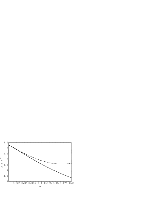
FIG. 15.: Numerical curve for $M(k)/\gamma$ (solid curve) as a function of $\gamma$ compared to the small $\gamma$ expansion (dashed curve) given in Eq. (C124). The vertical axis has the unit ${\rm R\!y}^{2}a_{0}^{3}$ and horizontal axis is dimensionless.

D Details of the exchange terms

We first examine the third term $T_{3}$ in Eq. (49). For this term $T_{3}$, only the “vacuum state” $|0\rangle$ (i.e. the tritium nucleus) contributes to the intermediate states when inserting a complete set of states just before the operator $N_{\bf p}(0)$. Hence,

$$T_{3} = \langle f|\psi^{\dagger}(0)|0\rangle{1\over E-E_{i}}\langle 0|N_{\bf p}(0)|i\rangle$$ (D1)

$$= -\phi_{f}^{*}(0){1\over E-E_{i}}\langle{\bf p}|\left\{{e^{2}\over 4\pi r}+v(r)\right\}|i\rangle\,,$$ (D2)

where $\langle{\bf p}|$ and $|i\rangle$ are the electron states of the final beta ray and the initial tritium atom. The Schrödinger equations for these energy eigenstates can be used to rewrite

$$T_{3}=-\phi_{f}^{*}(0)\langle{\bf p}|i\rangle\,.$$ (D3)

This is an exchange term which represents the amplitude for the electron produced by the weak interaction shaking the bound electron of the original tritium out and being bound by the final helium nucleus itself. We shall not evaluate $T_{3}$ because it is canceled by a piece of the exchange term $T_{\rm e}$ which we now turn to discuss.

The exchange part $T_{\rm e}$ in $T_{2}$ of Eq. (67) involves the ket $|i,{\bf r}_{2}{=}{\bf 0}\rangle$ For the evaluation of this exchange term, it is convenient to interchange the roles of $r_{1}$ and $r_{2}$ in Eqs. (69), (70) and (71) and define

$${\tilde{H}}_{1} = {{\bf p}_{1}^{2}\over 2m}-{e^{2}\over 4\pi r_{1}}\,,$$ (D4)

$${\tilde{H}}_{2} = {{\bf p}_{2}^{2}\over 2m}-{2e^{2}\over 4\pi r_{2}}\,,$$ (D5)

$${\tilde{H}}_{I} = {e^{2}\over 4\pi|{\bf r}_{1}-{\bf r}_{2}|}-{e^{2}\over 4\pi r_{1}}\,.$$ (D6)

This enables us to expand $T_{\rm e}$ in powers of ${\tilde{H}}_{I}$ as was done before [c.f. Eq. (73)]. The leading term in $T_{\rm e}$, which we now denote as $T_{\rm e}^{0}$, is

$$T_{\rm e}^{0}=\int(d^{3}{\bf r}_{1})\phi^{*}_{\bf p}({\bf r}_{1})\phi_{i}({\bf r}_{1})\langle f|\left[{e^{2}\over 4\pi|{\bf r}_{1}-{\bf r}_{2}|}-{2e^{2}\over 4\pi r_{1}}-v(r_{1})\right]{1\over{\tilde{H}}_{2}+E_{i}-E-E_{f}-i\epsilon}|{\bf r}_{2}{=}{\bf 0}\rangle\,,$$ (D7)

upon using the fact that $|i\rangle$ is an eigenstate of ${\tilde{H}}_{1}$. Noting that $\langle f|$ is an eigenstate of ${\tilde{H}}_{2}$, we may write

$$T_{\rm e}^{0} = \!\int(d^{3}{\bf r}_{1})\phi^{*}_{\bf p}({\bf r}_{1})\phi_{i}({\bf r}_{1})\langle f|\left({e^{2}\over 4\pi|{\bf r}_{1}{-}{\bf r}_{2}|}-{e^{2}\over 4\pi r_{1}}\right){1\over{\tilde{H}}_{2}{+}E_{i}{-}E{-}E_{f}{-}i\epsilon}|{\bf r}_{2}{=}{\bf 0}\rangle$$ (D9)

$$+{1\over E-E_{i}}\phi_{f}^{*}(0)\int(d^{3}{\bf r}_{1})\phi^{*}_{\bf p}({\bf r}_{1})\phi_{i}({\bf r}_{1})\left[{e^{2}\over 4\pi r_{1}}+v(r_{1})\right]\,.$$

The second term here exactly cancels $T_{3}$ in view of Eq. (D2).

To evaluate the sum $T_{\rm e}^{0}+T_{3}$, the first line in Eq. (D9), we follow the method of Appendix B in writing the denominator as the integral of an exponential, use the Heisenberg equation of motion with $\langle f|(\tilde{H}_{2}-E_{f})=0$, and express the Coulomb Green’s functions as Fourier integrals, to obtain

$$T_{\rm e}^{0}+T_{3} = e^{2}\!\int(d^{3}{\bf r}_{1})\phi^{*}_{\bf p}({\bf r}_{1})\phi_{i}({\bf r}_{1})\int_{0}^{\infty}dt\,e^{i(E-E_{i})t}$$ (D11)

$$\int{(d^{3}{\bf k})\over(2\pi)^{3}}{1\over k^{2}}e^{i{\bf k}\cdot{\bf r}_{1}}\langle f|\left(e^{-i{\bf k}\cdot{\bf r}_{2}(t)}-1\right)|{\bf r}_{2}{=}{\bf 0}\rangle\,.$$

In leading order, which is equivalent to the $p\to\infty$ limit, we may replace the outgoing beta electron wave function $\phi^{*}_{\bf p}({\bf r}_{1})$ by the free plane wave $e^{-i{\bf p}\cdot{\bf r}_{1}}$, neglect $E_{i}$ relative to $E=p^{2}/2m$, and replace ${\bf r}_{2}(t)$ by the free particle motion,

$${\bf r}_{2}(t)={\bf r}_{2}+{\bf p}t/m\,.$$ (D12)

Ordering the resulting exponential gives

$$e^{-i{\bf k}\cdot{\bf r}_{2}(t)}\simeq e^{-ik^{2}t/2m}e^{-it{\bf k}\cdot{\bf p}/m}e^{-i{\bf k}\cdot{\bf r}_{2}}\,.$$ (D13)

Since the momentum operator generates a spatial translation, we now arrive at

$$T_{\rm e}^{0}+T_{3} \simeq ie^{2}\!\int(d^{3}{\bf r}_{1})\int{(d^{3}{\bf k})\over(2\pi)^{3}}{1\over k^{2}}e^{-i({\bf p}-{\bf k})\cdot{\bf r}_{1}}\phi_{i}({\bf r}_{1})$$ (D15)

$$\int_{0}^{\infty}dt\,e^{ip^{2}t/2m}\left\{e^{-ik^{2}t/2m}\langle f|{\bf r}_{2}={\bf k}t/m\rangle-\langle f|{\bf r}_{2}{=}{\bf 0}\rangle\right\}\,.$$

To exhibit the leading order contribution, we change variables by writing

$${\bf k}={m\over t}{\bf r}\,,$$ (D16)

and

$$t={mr\over p}\tau\,,\qquad{\bf r}_{1}={\bf r}+{1\over p}{\bf u}\,.$$ (D17)

This change produces

$$T_{\rm e}^{0}+T_{3} \simeq i4\pi\eta^{3}a_{0}^{2}\!\int(d^{3}{\bf r}){1\over r^{2}}\int_{0}^{\infty}{d\tau\over\tau}e^{-i({\bf p}\cdot{\bf r}-pr/\tau)}$$ (D19)

$$e^{ipr\tau/2}\left\{e^{-ipr/2\tau}\phi_{f}^{*}({\bf r})-\phi_{f}^{*}({\bf 0})\right\}\int{(d^{3}{\bf u})\over(2\pi)^{3}}\phi_{i}({\bf r}+{\bf u}/p)e^{-i(\hat{\bf p}-\hat{\bf r}/\tau)\cdot{\bf u}}\,.$$

In the $p\to\infty$ limit, $\phi_{i}({\bf r}+{\bf u}/p)$ may be replaced by $\phi_{i}({\bf r})$, and we encounter

$$\int{(d^{3}{\bf u})\over(2\pi)^{3}}e^{-i(\hat{\bf p}-\hat{\bf r}/\tau)\cdot{\bf u}} = \delta^{(3)}(\hat{\bf p}-\hat{\bf r}/\tau)$$ (D20)

$$= \delta(1-\tau)\sum_{lm}Y_{lm}^{*}(\hat{\bf p})Y_{lm}(\hat{\bf r})\,,$$ (D21)

which produces

$$T_{\rm e}^{0}+T_{3}\simeq i4\pi\eta^{3}a_{0}^{2}\!\int(d^{3}{\bf r}){1\over r^{2}}\sum_{l^{\prime}m^{\prime}}Y_{l^{\prime}m^{\prime}}^{*}(\hat{\bf p})Y_{l^{\prime}m^{\prime}}(\hat{\bf r})\left\{\phi_{f}^{*}({\bf r})-e^{ipr}\phi_{f}^{*}({\bf 0})\right\}\phi_{i}({\bf r})\,.$$ (D22)

The last term involving $e^{ipr}\phi_{f}^{*}({\bf 0})$ vanishes in the large $p$ limit by virtue of its infinitely rapid phase oscillation. The angular part of the ${\bf r}$ integration just picks out the $l$ and $m$ values of the final atomic wave function,

$$\phi_{f}^{*}({\bf r})=R_{fl}^{*}(r)Y^{*}_{lm}(\hat{\bf r})\,.$$ (D23)

Accordingly, to the leading order, the exchange amplitude is given by

$$T_{\rm e}^{0}+T_{3}\simeq i\,4\pi\eta^{3}\,a_{0}^{2}\,Y_{lm}^{*}({\hat{\bf p}})\int_{0}^{\infty}drR_{fl}^{*}(r)\phi_{i}(r)\,,$$ (D24)

which is of order $\eta^{3}$.

Although the amplitude (D24) is of order $\eta^{3}$, it contributes to the decay rate only through the order $\eta^{4}$. For $l{\not=}0$, this result is of order $\eta^{2}$ relative to the leading direct result (136) which is of order $\eta$. Therefore the exchange effect gives a correction to the decay rate at order $\eta^{4}$. For case $l=0$, the leading exchange amplitude (D24) is relatively imaginary. Since the leading imaginary amplitude appears at the order $\eta$, the exchange correction to the decay rate is only of order $\eta^{4}$ We note here that this contradicts with the results in the literature [14], where the dominant exchange amplitudes appear in order $\eta^{4}$.

REFERENCES

• [1] J. F. Wilkerson, Nucl. Phys. B 31 (Proc. Suppl.) (1993), 32.
• [2] R. G. H. Robertson et al., Phys. Rev. Lett. 67 (1991), 957.
• [3] E. Holzschuh et al., Phys. Lett. B 287 (1992), 381.
• [4] H. Kawakami et al., Phys. Lett. B 256 (1991), 105.
• [5] W. Stoeffl, Bull. Am. Phys. Soc. 37 (1992), 925; D. J. Decman and W. Stoeffl, presented at conf. The Many Aspects of Neutrino Physics, Fermilab, Nov. 1991 (unpublished); W. Stoeffl and D. J. Decman, Proceedings of XXVIIIth Rencontre De Moriond Workshop, Villars sur Ollon, Switzerland, Jan 30 - Feb 6, 15 (1993); W. Stoeffl and D. J. Decman, Anomalous Structure in the Beta Decay of Gaseous Molecular Tritium, UCRL-JC-115771/Preprint, (Phys. Rev. Lett., to be published).
• [6] H. Backe et al., Phys. Scr. T 22 (1988), 98; A. Picard et al., Nucl. Instr. and Methods in Phys. Research B63 (1992), 345; Ch. Weinheimer, et al., Phys. Lett. B 300 (1993), 210.
• [7] D. A. Knapp, Los Alamos Ph. D. thesis, (1986).
• [8] R. L. Martin and J. S. Cohen, Phys. Lett. A 110 (1985), 95; O. Fackler, B. Jeziorski, W. Lolos, J. J. Monkhorst, and K. Szalewica, Phys. Rev. Lett. 55 (1985), 1388; H. Agren and V. Carravetta, Phys. Rev. A 38 (1988), 2707.
• [9] D. H. Wilkinson, Nucl. Phys. A 526 (1991), 131; J. J. Simpson, Phys. Rev. D 23 (1981), 649.
• [10] R. G. H. Robertson and D. A. Knapp, Ann. Rev. Nucl. Part. Sci. 38 (1988), 185.
• [11] L. Durand and J. L. Lopez, Phys. Lett. B 198 (1987), 249; J. L. Lopez and L. Durand, Phys. Rev. C 37 (1988), 535.
• [12] E. G. Drukarev and M. I. Strikman, Zh. Eksp. Teor. Fiz. 91 (1986), 1160 [Sov. Phys. — JETP 64 (1986), 686].
• [13] M. E. Rose, Phys. Rev. 49 (1936), 727.
• [14] J. N. Bahcall, Phys. Rev. 129 (1963), 2683.
• [15] See, for example, L. S. Brown, “Quantum Field Theory,” pp. 219-298, Cambridge University Press, 1992.
• [16] See, for example, K. Gottfried, “Quantum Mechanics,” section 17, W. A. Benjamin, Inc., New York, 1966. Notice that our wave function differs from the wave function there by a factor $(2\pi)^{3/2}$ due to different normalization, and our radial wave function $R_{kl}(r)$ is denoted by $C_{l}(k;r)$ there.
• [17] For the integral representation of the confluent hypergeometric function, see, for example, L. D. Landau and E. M. Lifshitz, “Quantum Mechanics,” 2nd ed., p. 602, Pergamon Press, 1965. The formulas we need are (d.8) and (d.9), p. 602.