BNL-61907

ISU-HET-95-4

June, 1995

LIMITS ON NON STANDARD TOP QUARK COUPLINGS FROM ELECTROWEAK MEASUREMENTS

S. Dawson^(a) and G. Valencia^(b)
(a) Physics Department, Brookhaven National Laboratory, Upton, NY 11973
^(b) Department of Physics, Iowa State University, Ames IA 50011

We calculate the typical size of loop corrections to electroweak observables arising from non-standard $Z{\overline{t}}t$ and $Wtb$ vertices. We use an effective Lagrangian formalism based on the electroweak gauge group $SU(2)_{L}\times U(1)_{Y}\rightarrow U(1)_{EM}$. Limits on the non-standard model top quark couplings from electroweak observables are presented and compared with previously obtained limits.

1 Introduction

The large mass of the recently discovered top quark suggests that the top quark is fundamentally different from the five lighter quarks. A number of models have been proposed in which the interactions of the top quark are responsible for the $SU(2)_{L}\times U(1)_{Y}$ electroweak symmetry breaking [1, 2]. In this note, we make a model-independent study of the limits on the couplings of the third generation quarks to gauge bosons which can be inferred from the LEP and SLC data.

Precision electroweak measurements at LEP and SLC offer a window into the $Z{\overline{t}}t$ and $Wtb$ couplings since these couplings appear in loop corrections to the $Z$ decay widths. Rare $B$ and $K$ decays such as $b\rightarrow s\gamma$ can also probe the $Wtb$ coupling [3], while in the future, the $Wtb$ coupling can perhaps be measured to an accuracy of around $30\%$ at the Tevatron through single top production [4] .

As has been emphasized recently [5], the determination of $\alpha_{s}(M_{Z})$ at LEP is somewhat higher than that obtained from low energy measurements such as deep inelastic scattering. The existence of new non-standard model physics will affect the extraction of $\alpha_{s}$ at the $Z$ pole and in many cases will lower it to be in agreement with the low energy data [6, 7].

We consider a picture in which the new physics responsible for the electroweak symmetry breaking is at some high scale, $\Lambda>4\pi v\sim 3~{}TeV$. In this case, the physics at low energy can be written in terms of an effective Lagrangian describing the interactions of the $SU(2)_{L}\times U(1)_{Y}$ gauge fields with the Goldstone bosons which become the longitudinal components of the $W$ and $Z$ gauge bosons. It is straightforward to incorporate fermions into this picture [4, 8, 9]. We will not concern ourselves with the source of the new physics–it could be supersymmetry, technicolor, top color, or something else entirely. The only important point is that the new physics occurs at a high scale, so that an expansion in powers of $M_{Z}^{2}/\Lambda^{2}$ is appropriate.

2 Effective Lagrangian

In this note, we assume that whatever is responsible for generating the non-standard model top quark couplings occurs at a high scale (perhaps $\Lambda\sim 3~{}TeV$) and so the use of a non-linear effective Lagrangian is appropriate. This Lagrangian can be used to describe the electroweak sector of the theory at low energy. We will assume that only the top quark couplings are non-standard; the case of non-standard $b$- quark couplings to the $Z$ has been examined by many authors [11]. If we consider the gauge group $SU(2)_{L}\times U(1)_{Y}$ broken to $U(1)_{EM}$, then there are $3$ Goldstone bosons, $\omega_{i}$, which eventually become the longitudinal components of the $W^{\pm}$ and $Z$ gauge bosons. The minimal Lagrangian which describes the interactions of the $SU(2)_{L}\times U(1)_{Y}$ gauge bosons with the Goldstone bosons has been given in [12]. This non-renormalizable Lagrangian is interpreted as an effective field theory, valid below some scale $\Lambda$ and yields the gauge boson self interactions that we use in this calculation [9].

In a similar way one can write an effective Lagrangian that describes the interactions of fermions to the electroweak gauge bosons. The terms that are needed for our calculation have been described in the literature [8] and in unitary gauge they are:

$${\cal L}_{\rm eff} = -{g\over 2\cos\theta_{W}}\biggl{[}(L_{t}+\delta L_{t}){\overline{t}}_{L}\gamma^{\mu}t_{L}+(R_{t}+\delta R_{t}){\overline{t}}_{R}\gamma^{\mu}t_{R}\biggr{]}Z_{\mu}$$ (1)

$$-\biggl{\{}{g\over\sqrt{2}}\biggl{[}(1+\delta\kappa_{L}){\overline{t}}_{L}\gamma^{\mu}b_{L}+(\delta\kappa_{R}){\overline{t}}_{R}\gamma^{\mu}b_{R}\biggr{]}W_{\mu}^{+}+h.c.\biggr{\}}$$

where we use the standard notation $t_{L,R}=(1\mp\gamma_{5})/2t$, $L_{t}=1-4/3s_{Z}^{2}$, $R_{t}=-4/3s_{Z}^{2}$. We have assumed that the new interactions are CP conserving and so there are 4 new real parameters to be examined: $\delta L_{t}$, $\delta R_{t}$, $\delta\kappa_{L}$, and $\delta\kappa_{R}$. We will use Eq. 1 at one-loop, but we will not consider other anomalous couplings that may act as counterterms to this one-loop calculation. Therefore, our results will not constitute strict bounds on the parameters of Eq. 1, but instead they will depend on the naturalness assumption that contributions from different couplings do not cancel each other. For example, we do not discuss possible flavor changing neutral current couplings.

3 Limits from Electroweak data

Possible effects of new physics at LEP and SLC from non-standard $t$-quark couplings can be parameterized in terms of the $4$ parameters $S$, $T$, $U$, and $\delta_{b{\overline{b}}}$ [14]. The parameters $S$, $T$, and $U$ describe the effects of the new physics on the gauge boson two point functions, while $\delta_{b{\overline{b}}}$ contains the non-oblique corrections to the $Z\rightarrow b{\overline{b}}$ decay rate. The non-standard top quark couplings do not generate non-oblique corrections to decay rates other than $Z\rightarrow b\overline{b}$.

We perform a one-loop calculation of these effects and retain terms linear and quadratic in the small parameters ($\delta\kappa_{L},\delta\kappa_{R},\delta L_{t}$, and $\delta R_{t}$). Of course, our formalism is based on the assumption that the new couplings are small corrections to the minimal standard model couplings and thus the linear terms dominate the quadratic terms whenever our formalism is valid. We keep the quadratic terms only because there is one coupling that does not contribute linearly to the processes in question. Since the bounds we obtain are based on naturalness assumptions, among them that there are no cancellations between different contributions to the physical observables, they can be applied to this quadratic term as well.

Our one loop calculation including the new couplings is divergent. In the language of effective field theories these divergences would be absorbed by higher dimension counterterms. We will make use of the divergent terms to place bounds on the couplings by examining the leading non-analytic contribution to the amplitudes as discussed in Ref. [9]. To this effect we first regularize the integrals in $n=4-2\epsilon$ space-time dimensions. The coefficient of $1/\epsilon$ is also the coefficient of the term $\log\mu^{2}$ and thus gives the leading non-analytic term. The use of these terms as estimates for the size of counterterms has been emphasized in Ref. [10].

The caveats discussed in Ref. [9] apply here as well: our bounds are valid only as order of magnitude estimates. They are also based on the assumption that terms induced by different couplings do not cancel against each other. In other words, the LEP observables do not directly measure the coefficients in Eq. 1 and it is only from naturalness arguments that we can place limits on the anomalous top quark couplings. For this reason our bounds are not a substitute for direct measurements in future high energy machines.

In order to obtain limits we use the fit of Ref. [7] to possible “new physics” contributions to $S$,$T$, $U$, and $\delta_{b{\overline{b}}}$. This fit assumes $M_{t}=175\pm 16~{}GeV$ and gives:

$$S_{\rm NEW}^{exp} = -.21\pm.24^{-.08}_{+.17}$$

$$T_{\rm NEW}^{exp} = -.09\pm.32^{+.16}_{-.11}$$

$$U_{\rm NEW}^{exp} = -.53\pm.61$$

$$\delta_{b{\overline{b}},{\rm NEW}}^{exp} = .022\pm.011\quad.$$

The standard model top quark and Higgs boson contributions are ${\bf{\it not}}$ included in the “new physics” contributions. The central values in Eq. LABEL:langnum are for $M_{H}=300~{}GeV$, the upper second errors are the differences when $M_{H}=1~{}TeV$, while the lower second errors take $M_{H}=60~{}GeV$.

Refs. [4, 8, 13] computed the contributions of ${\cal O}({M_{t}^{2}/M_{W}^{2}})$ to $T$ and $\delta_{b{\overline{b}}}$. Here we extend that calculation to include all the leading non-analytic terms, even those not enhanced by $M_{t}^{2}/M_{W}^{2}$. We find

$$S_{\rm NEW} = {1\over 3\pi}\biggl{[}2\delta R_{t}-\delta L_{t}-{3\over 2}(\delta L_{t}^{2}+\delta R_{t}^{2})\biggr{]}\log({\mu^{2}\over M_{Z}^{2}})$$

$$T_{\rm NEW} = {3\over 4\pi s_{Z}^{2}}\biggl{(}{M_{t}\over M_{W}}\biggr{)}^{2}\biggl{[}\delta\kappa_{L}+{\delta\kappa_{L}^{2}+\delta\kappa_{R}^{2}\over 2}+\delta R_{t}-\delta L_{t}$$

$$-{(\delta L_{t}-\delta R_{t})^{2}\over 2}\biggr{]}\log({\mu^{2}\over M_{Z}^{2}})$$

$$U_{\rm NEW} = {1\over\pi}\biggl{[}-2\delta\kappa_{L}-(\delta\kappa_{L}^{2}+\delta\kappa_{R}^{2})+\delta L_{t}+{\delta L_{t}^{2}+\delta R_{t}^{2}\over 2}\biggr{]}\log({\mu^{2}\over M_{Z}^{2}})$$

$$\delta_{b{\overline{b}},{\rm NEW}} = {\alpha\over 9\pi}{1\over L_{B}^{2}+R_{B}^{2}}\biggl{\{}{3(4s_{Z}^{4}-18s_{Z}^{2}+9)\over 4s_{Z}^{2}\cos 2\theta_{W}}{M_{t}^{2}\over M_{W}^{2}}\biggl{[}-{(\delta R_{t}-\delta L_{t})^{2}\over 2}+{\delta\kappa_{L}^{2}\over 2}+\delta\kappa_{L}\biggr{]}$$ (3)

$$+{3\over 4s_{Z}^{2}\cos 2\theta_{W}}{M_{t}^{2}\over M_{W}^{2}}\biggl{[}\delta L_{t}(4s_{Z}^{4}+2s_{Z}^{2}-3)-{\delta\kappa_{R}^{2}\over 2}(28s_{Z}^{4}+2s_{Z}^{2}-9)$$

$$+{\delta R_{t}\over 2}(4s_{Z}^{4}-28s_{Z}^{2}+15)\biggr{]}+{4s_{Z}^{2}-3\over 3\cos 2\theta_{W}}\biggl{(}2\delta R_{t}-\delta L_{t}-{3\over 2}(\delta L_{t}^{2}+\delta R_{t}^{2})\biggr{)}$$

$$+{(16s_{Z}^{2}-17)\over 4c_{Z}^{2}s_{Z}^{2}}\biggl{[}\biggl{(}{\delta\kappa_{L}^{2}\over 2}+\delta\kappa_{L}\biggr{)}(2s_{Z}^{2}-3)+\delta\kappa_{R}^{2}\biggr{]}\biggr{\}}\log({\mu^{2}\over M_{Z}^{2}}),$$

where $L_{B}=-1+2/3s_{Z}^{2}$ and $R_{B}=2/3s_{Z}^{2}$. We have not included contributions that are independent of $\delta\kappa_{L}$, $\delta\kappa_{R}$, $\delta L_{t}$, or $\delta R_{t}$. These were the subject of Ref. [9].

As discussed in Ref. [9], we choose as input parameters for our renormalization scheme $G_{F}$, $M_{Z}$ and $\alpha(M_{Z})=1/128.8$. In this scheme $M_{W}$ and $s_{Z}^{2}$ are derived quantities. Numerically:

$$\delta_{b{\overline{b}}} = {\alpha\over\pi}\biggl{\{}{M_{t}^{2}\over M_{W}^{2}}\biggl{[}-2.29\biggl{(}(\delta R_{t}-\delta L_{t})^{2}-\delta\kappa_{L}^{2}-2\delta\kappa_{L}\biggr{)}$$ (4)

$$+3.19\delta\kappa_{R}^{2}-2.11\delta L_{t}+3.96\delta R_{t}\biggr{]}+.29(\delta R_{t}^{2}+\delta L_{t}^{2})+.19(\delta L_{t}-2\delta R_{t})$$

$$-.65\delta\kappa_{R}^{2}+3.57(\delta\kappa_{L}^{2}+2\delta\kappa_{L})\biggr{\}}\log({\mu^{2}\over M_{Z}^{2}})\quad.$$

The anomalous couplings are assumed to be small, so we will retain only the linear couplings with the exception of $\delta\kappa_{R}$ as mentioned before. We follow the philosophy of Ref. [10] in our use of the leading non-analytic terms. Accordingly, we must choose a renormalization scale below the scale of new physics $\Lambda\approx 3~{}TeV$ in such a way that the logarithms are of order one. With the prejudice that these new couplings are somehow related to the top-quark mass, we choose for our estimates $\mu=2M_{t}$. Using $M_{t}=175\pm 16~{}GeV$ we find the $90\%$ confidence level limits:

• From $U^{exp}_{\rm NEW}$: $-2<-2\delta\kappa_{L}+\delta L_{t}<.6$

• From $S^{exp}_{\rm NEW}$: $-2<2\delta R_{t}-\delta L_{t}<1$

• From $T^{exp}_{\rm NEW}$ : $-.06<\delta\kappa_{L}+\delta R_{t}-\delta L_{t}<.05$

• From $\delta_{b\overline{b},{\rm NEW}}^{exp}$: $.02<\delta\kappa_{L}-.3\delta L_{t}+.6\delta R_{t}<.2$

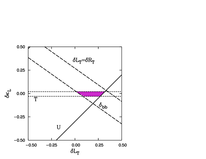
Figure 1: $90\%$ confidence level bounds from electroweak data with $\mu=2M_{t}$. The region enclosed by the dotted and dashed lines are the limits from $T^{exp}_{\rm NEW}$ and $\delta_{b{\overline{b}},{\rm NEW}}^{exp}$ respectively. For $\delta L_{t}=\delta R_{t}$, the limit from $S^{exp}_{\rm NEW}$ is $-2<\delta L_{t}<1$. The region above the solid line is allowed by $U^{exp}_{\rm NEW}$. The region allowed by all measurements is shaded.

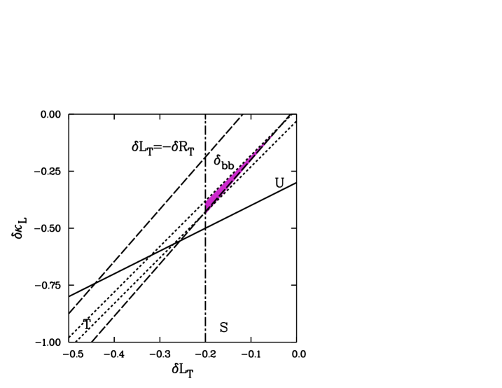
Figure 2: $90\%$ confidence level bounds from electroweak data with $\mu=2M_{t}$. The regions enclosed by the dotted and dashed lines are the limits from $T^{exp}_{\rm NEW}$ and $\delta_{b{\overline{b}},{\rm NEW}}^{exp}$ respectively. The region to the right of the dot-dashed line is allowed from $S^{exp}_{\rm NEW}$, while the region above the solid line is allowed by $U^{exp}_{\rm NEW}$.

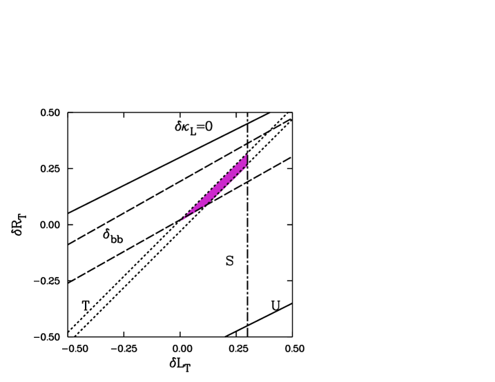
Figure 3: $90\%$ confidence level bounds from electroweak data with $\mu=2M_{t}$. The regions enclosed by the dotted and dashed lines are the limits from $T^{exp}_{\rm NEW}$ and $\delta_{b{\overline{b}},{\rm NEW}}^{exp}$ respectively. The region to the left of the dot-dashed line is allowed from $U^{exp}_{\rm NEW}$, while the region below the solid line is that allowed by $S^{exp}_{\rm NEW}$. The region allowed by all measurements is shaded.

In Fig. 1, we take $\delta L_{t}=\delta R_{t}$ and show the limits on $\delta\kappa_{L}$ as a function of $\delta L_{t}$. Including the limit from $U^{exp}_{\rm NEW}$ excludes a considerably larger region of parameter space than would be excluded from $T^{exp}_{\rm NEW}$ and $\delta_{b{\overline{b}},{\rm NEW}}^{exp}$ alone. If the new couplings modify only the axial coupling to the $Z$, ${\cal L}\sim\overline{t}\gamma^{\mu}\gamma_{5}tZ_{\mu}$, then $\delta L_{t}=-\delta R_{t}$. We show the limits in this case in Fig. 2 and see that only a small region of parameter space is allowed. This agrees with previous observations that the electroweak data tend to prefer $\delta L_{t}=\delta R_{t}$ [4]. In Fig. 3, we set $\delta\kappa_{L}=0$ and show the $90\%$ confidence level bounds on $\delta L_{t}$ and $\delta R_{t}$. In this figure, we again see the trend that in the allowed region, $\delta L_{t}\sim\delta R_{t}$. In all three figures, it is interesting to note the role of the limit on $U^{exp}_{\rm NEW}$, which is more significant than the limit from $S^{exp}_{\rm NEW}$.

The effects of a possible right-handed coupling of the $W$ to the $b$ and $t$ first arises at ${\cal O}(\delta\kappa_{R}^{2})$ in $Z$ decays. The best limit comes from $T_{\rm NEW}^{exp}$ and is

$$\mid\kappa_{R}\mid<.3\quad.$$ (5)

This is considerably weaker than the limit from the CLEO measurement of $b\rightarrow s\gamma$[3].

$$-.05<{\delta\kappa_{R}\over\mid V_{tb}\mid}<.01\quad.$$ (6)

4 Conclusions

The increasing precision of electroweak measurements, along with the recent measurement of the top quark mass, allows limits to be placed on the non-standard model couplings of the top quark to gauge bosons. We have updated previous limits by including terms not enhanced by the top quark mass. These additional terms allow a larger region of parameter space to be excluded than in previous studies.

It is interesting to speculate as to the size of these coefficients in various models. If the non-standard couplings arise from loop effects then they might be expected to have a size $\sim{\alpha\over\pi}\sim.002$, several orders of magnitude smaller than the current limits. In models where the non-standard couplings arise from four-fermion operators at a high scale, the coefficients have a typical size [13],

$$\delta L_{t}\sim{3g_{A}\over 8\pi^{2}}{M_{t}^{2}\over\Lambda^{2}}\log\biggl{(}{\Lambda^{2}\over M_{t}^{2}}\biggr{)}\quad.$$ (7)

In the top color model of Ref. [13], $g_{A}\sim 4\pi(.11)$ and so a scale $\Lambda\sim 2~{}TeV$ would yield a coefficient, $\delta L_{t}\sim 10^{-3}$. Unfortunately, unlike the case with the b-quark couplings, the limits on top quark couplings do not yet seriously constrain model building.

References

- [1] W. Bardeen, C. Hill, and M. Lindner, Phy. Rev. D41 (1990) 1647; C. Hill, Phys. Lett. B266 (1991) 419; S. Martin, Phys. Rev. D46 (1992) 2197; Phys. Rev. D45(1992) 4283; Nucl. Phys. B398 (1993) 359; M. Lindner and D. Ross, Nucl. Phys. B370 (1992) 30; R. Bonisch, Phys. Lett. B268 (1991) 394; C. Hill, D. Kennedy, T. Onogi, and H. Yu, Phys. Rev. D47 (1993) 2940
- [2] C. Hill, Phys. Lett. B345 (1995) 483; E. Eichten and K. Lane, BUHEP-95-11, hep-ph/9503433, March, 1995.
- [3] K. Fukikawa and A. Yamada, Phys. Rev. D49 (1994) 5890; J. Hewett and T. Rizzo, Phys. Rev. D49 (1994) 319.
- [4] K. Whisnant, B. L. Young and X. Zhang, Phys. Rev. D52 (1995) 3115; E. Malkawi and C.-P. Yuan, Phys. Rev. D50 (1994) 4462; D. Carlson, E. Malkawi, and C.-P. Yuan, Phys. Lett. B337 (1994) 145.
- [5] M. Shifman, Mod. Phys. Lett. A10 (1995) 605.
- [6] S. Catani, DFF- 211/10/94, hep-ph/9411361, November, 1994; P. Chankowski and S. Pokorski, IFT-UW-95/5, hep-ph/9505304, May, 1995; G. Kane, R. Stuart, and J. Wells, UM-TH-95-16, hep-ph/9505207, April, 1995.
- [7] J. Erler and P. Langacker, Phys. Rev. D50 (1994) 1304.
- [8] R. Peccei and X. Zhang, Nucl. Phys. B337 (1990) 269; R. Peccei, S. Peris, and X. Zhang, Nucl. Phys. B349 (1991) 305.
- [9] S. Dawson and G. Valencia, Nucl. Phys. B439 (1995) 3.
- [10] A. Manohar and H. Georgi, Nucl. Phys. B234 (1984) 189.
- [11] R. Holdom, R. Chivukula, S. Selipsky, and E. Simmons, Phys. Rev. Lett. 69 (1992) 575; R. Chivukula, E. Simmons, and J. Terning, Phys. Lett. B331 (1994) 383; G.-H. Wu,Phys. Rev. Lett. 74 (1995) 4137; D. Schaile and P. Zerwas, Phys. Rev. 45 (1992) 3263.
- [12] A. Longhitano, Nucl. Phys. B188 (1981) 118.
- [13] X. Zhang, Mod. Phys. Lett. A9 (1994) 1955; C. Hill and X. Zhang, Phys. Rev. D51 (1995) 3563.
- [14] D. C. Kennedy and B. W. Lynn, Nucl. Phys. 322 (1989) 1; M. Peskin and T. Takeuchi, Phys. Rev. Lett. 65 (1990) 964; Phys. Rev. D46 (1992) 381; G. Altarelli, and R. Barbieri, and F. Caravaglios, Nucl. Phys. 405 (1993) 3.