We analyze the large-order behaviour in perturbation theory of classes of diagrams with an arbitrary number of chains (i.e. photon lines, dressed by vacuum polarization insertions). We derive explicit formulae for the leading and subleading divergence as $n\to\infty$, and a complete result for the vacuum polarization at the next-to-leading order in $1/N_{f}$. In general, diagrams with more chains yield stronger divergence. We define an analogue of the familiar diagrammatic $R$-operation, which extracts ultraviolet renormalon counterterms as insertions of higher-dimension operators. We then use renormalization group equations to sum the leading $(\ln n/N_{f})^{k}$-corrections to all orders in $1/N_{f}$ and find the asymptotic behaviour in $n$ up to a constant that must be calculated explicitly order by order in $1/N_{f}$.

submitted to Nuclear Physics B

1 Introduction

Perturbative calculations in quantum field theories involve integrations over arbitrarily small distances and typically lead to divergent results. A finite result is obtained, when a theory is first regulated and counterterms are added to the bare Lagrangian ${\cal L}_{0}$. The Green functions computed from

$${\cal L}={\cal L}_{0}(\Lambda)+{\cal L}^{(4)}_{\rm ct}(\Lambda)$$ (1.1)

have perturbative expansions free from divergences order by order in the renormalized coupling $\alpha(\mu)$ so that they are finite in the limit when the cut-off $\Lambda$ is removed. A justification for this rather ad hoc-looking procedure can be obtained from the philosophy of ‘effective field theories’: Only the renormalized parameters are accessible to low-energy experiments and the apparently divergent regions of integration are in fact (almost) insignificant.

From the beginnings of renormalized quantum field theory it has been recognized that the Green functions (in the limit $\Lambda\to\infty$) obtained in this way can not be unambiguously defined (as certain analytic functions in a neighbourhood of $\alpha=0$) through their perturbative expansions alone, because they diverge for any $\alpha\neq 0$ [1]. Although from a practical point of view one may consider these expansions as asymptotic (to nature), the (non-perturbative) existence of renormalized field theories remains a mathematically largely unsolved problem, the divergence of perturbative expansions being one face of this problem, the issue of triviality in non-asymptotically free theories being another.

Without touching the profound problem of existence, the behaviour of perturbative expansions as formal series is itself important. In considering the perturbative expansion to all orders, one takes in fact a glimpse beyond perturbation theory. Thus, although the questions of triviality and Landau poles in general can not be answered without knowledge of non-perturbative properties of the theory, some aspects can be investigated strictly within perturbation theory. In theories where the coupling can become large at low energies, the details of the divergence of the perturbation series may provide some hints to selecting the numerically most important corrections already in moderately large orders. The dominant source of divergence (at least with present knowledge) was identified by Lautrup [2] and ‘t Hooft [3], who investigated a particular class of diagrams with an arbitrary number of vacuum polarization insertions into a single gauge boson line in a loop diagram. The sum of these diagrams has the generic behaviour

$$\Gamma(\underline{p},\mu,\alpha(\mu))=\sum_{n}K\left(\frac{\beta_{0}}{a}\right)^{n}n!\,n^{b}\alpha(\mu)^{n+1}\left[1+{\cal{O}}\!\left(\frac{1}{n}\right)\right]\,.$$ (1.2)

Here $\underline{p}$ is a collection of external momenta and $\beta_{0}$ is the first coefficient of the $\beta$-function. With the definition given later, the constant $a$ is integer (and sometimes half-integer). The $n!$-behaviour arises as a consequence of renormalization and for this reason has become known as renormalon divergence. Note that the term ‘divergence’ is applied to the divergence of the perturbation series as well as to the divergences of Feynman integrals, which are subtracted in the process of renormalization.

In strictly renormalizable theories the coupling depends logarithmically on the renormalization scale $\mu$ and each vacuum polarization loop gives a $\ln k^{2}/\mu^{2}$. This logarithm is large whenever the loop momentum $k$ is very different from $\mu$. In the present paper we consider only large momentum regions $k\gg\mu$ and ultraviolet (UV) renormalons, with $a>0$. The divergences associated with regions of integration over large loop momenta, like ${\mbox{d}}^{4}k/k^{4}$ for large $k$, are removed by the familiar renormalization procedure. The ultraviolet renormalons occur when a large power of $\ln k^{2}/\mu^{2}$ is integrated over the remaining ultraviolet regions of the subtracted integrands. In particular, the strongest divergence ($a=1$) is exclusively due to the remaining behaviour ${\mbox{d}}^{4}k/k^{6}$ for large $k$. The fact that UV renormalons are related to the large momentum expansion of Feynman integrands is crucial for their understanding, since it allows to describe UV renormalon divergence in large orders in terms of local operators just as explicit divergences in finite orders in the usual framework of renormalization. This observation is the basis for Parisi’s hypothesis [4] that UV renormalons can be removed by adding higher dimensional operators to the Lagrangian. In particular, the leading UV renormalon ($a=1$) could be compensated by an additional term

$${\cal L}_{\rm ct}^{(6)}=\frac{1}{\mu^{2}}\sum_{i}E_{i}(\alpha(\mu))\,{\cal O}_{i}\,,$$ (1.3)

where the sum runs over all local operators ${\cal O}_{i}$ of dimension six. To compensate all UV renormalons an infinite series of higher-dimensional operators would have to be added to the Lagrangian. In this paper we deal explicitly only with the leading UV renormalon and restrict ourselves to operators of dimension six.

The fact that the removal of ultraviolet renormalons, as the removal of ultraviolet divergences, can be formulated at the level of counterterms in the Lagrangian implies their universality: Once the coefficients $E_{i}$ have been determined from a suitable set of Green functions, the subtraction of the first ultraviolet renormalon is automatic for all Green functions. Another consequence is that the $E_{i}$ satisfy renormalization group equations, because Green functions with operator insertions satisfy them. These considerations fix the constant $b$ in eq. (1.2) [4]. The solution of the renormalization group equation depends on a boundary value which remains unconstrained by general considerations and is related to the normalization $K$ of the renormalon divergence in eq. (1.2).

An alternative approach, based on the Lagrangian at a finite cut-off rather than the renormalized Lagrangian, has been taken in [5]. The idea is that, since UV renormalons arise as a consequence of the infinite cut-off limit, their information is encoded in the large-cut-off expansion. Viewed in this way the compensation of UV renormalons bears close resemblance to Symanzik improvement of lattice actions [6].

Although the absence of the first ultraviolet renormalon as a consequence of eq. (1.3) seems rather obvious from the physical origin of UV renormalons, it has not yet been rigorously established. Moreover, the diagrammatic interpretation of eq. (1.3) is rather unclear: It does not give a clue, which diagrams contribute to the coefficients $E_{i}$ or whether they can be calculated at all in a systematic way. These are the questions which we address in this paper.

The diagrammatic study of UV renormalons received new attention only recently, through the work of Zakharov [7] and others [8–11]. The main difficulty that the diagrammatic approach has to face is that, because the object is to study perturbative expansions in large (that is, to all) orders, there is in fact no natural expansion parameter that would select a manageable subset of the infinity of all diagrams. In abelian gauge theory it is useful to classify diagrams in terms of complete gauge boson propagators. In first approximation, where only the first coefficient in the $\beta$-function is kept, the complete photon propagator reduces to a ‘chain’, a string of fermion loops. With few exceptions, previous investigations of UV renormalons have focused on diagrams with a single chain. In [12] it was shown that at this level one could remove the first ultraviolet renormalon from Green functions by counterterms of the form of eq. (1.3). The full complexity of calculating the normalization $K$ is already exhibited by diagrams with one complete photon propagator: To obtain the value of $K$, one can not approximate the propagator by a string of fermion loops (chain). The exact photon propagator has to be kept [10, 13]. For practical purposes this is equivalent to the statement that $K$ can not be calculated exactly.

An important new insight comes from the work of Vainshtein and Zakharov [14], who investigated the dominant contributions to the large-order behaviour of the photon vacuum polarization from diagrams with two chains by making direct use of the fact that the UV renormalons originate from the large-momentum regions in loops. The diagrams with two chains display a qualitatively new behaviour, because the four-fermion operators that appear in eq. (1.3) do not contribute to diagrams with a single chain. After insertion into the photon vacuum polarization, they were found to yield the dominant large-order behaviour.

In this paper we approach UV renormalons from an entirely diagrammatic perspective within the expansion in the number of chains, or, to be precise, in $1/N_{f}$, where $N_{f}$ is the number of fermions. Guided by the interpretation of UV renormalon divergence as similar to the usual ultraviolet divergences, we proceed in close analogy with the usual renormalization program. We will see that the analysis of UV renormalon divergence order by order in the expansion in chains has much in common with the analysis of UV divergence order by order in the coupling $\alpha$. The UV renormalon problem then takes a form similar to usual UV divergences: While certain properties like locality of counterterms and renormalization group equations can be established to all orders (for an arbitrary number of chains), the actual calculation of counterterms is limited to a few first terms because of the increasing complexity of integrals. In the present paper we proceed heuristically and do not give proofs which could be worked out as generalizations of standard cumbersome proofs of renormalization theory. Rather than giving proofs we describe the properties of regularized Feynman integrals and subtraction operators which would be essential ingredients to these proofs and illustrate how the extraction of ultraviolet renormalon divergence works in a number of examples.

Let us make a remark on the framework of the expansion in the number of chains: It might appear inconsequent to replace one expansion (the one in the coupling $\alpha$) by another. Our attitude is that this expansion can shed some light on the organization of UV renormalon divergence in the same way as, for instance, the $1/N_{c}$-expansion in QCD may reveal some information on the strong-coupling regime. In addition, we will see that the dominant UV renormalon divergences in each order of $1/N_{f}$ can be resummed to all orders in $1/N_{f}$ by solving the renormalization group equations. It is possible that the conclusions drawn from the $1/N_{f}$-expansion are not valid for any finite $N_{f}$ or valid only in a finite range of $N_{f}$. However, in an abelian gauge theory we do not consider this a likely possibility and rather expect a smooth continuation from the large-$N_{f}$ limit to small $N_{f}$.

In Sect. 2 we begin with detailing the expansion in chains. We introduce the Borel transform as generating function of perturbative coefficients and show how the factorial divergence of perturbation theory is encoded in the singularities of analytically regularized Feynman integrals. We collect some of their properties and classify the subgraphs that can contain the dominant UV renormalon. The extraction of the renormalon divergence then reduces to the extraction of pole parts of analytically regularized Feynman integrals at certain positions in regularization parameter space.

In Sect. 3 we construct an operation that picks out the terms with the largest number of singular factors. The leading large-$n$ behaviour at any order in $1/N_{f}$ is then found by successive extraction of pole parts of one-loop integrals. Beyond the leading large-$n$ behaviour it is essential to apply the method of infrared rearrangement [15, 16]. The operations introduced in this section are illustrated by the simplest example of the fermion self-energy up to two chains. In Sect. 4 we compute the fermion-photon vertex and the photon vacuum polarization including all diagrams with two chains and those diagrams with three chains that contain an additional fermion loop.

The universality of UV renormalons becomes most transparent by elevating the diagrammatic subtractions to the level of counterterms in the Lagrangian. We formulate the results of the previous sections in this language in Sect. 5. The renormalization group equations for Green functions with operator insertions are then used to sum the leading UV renormalon singularities to all orders in $1/N_{f}$. We summarize in Sect. 6 and discuss further applications of the formalism.

The derivation of some results quoted in sections 2 and 3 is collected in an appendix.

2 Renormalons and analytic regularization

In this section we set up the reorganization of the perturbation series in terms of chains and derive the Feynman rules for the Borel transform of this expansion. We show how renormalons are related to the singularities of analytically regularized Feynman integrals. We consider only the abelian gauge theory (QED) with Lagrangian

$${\cal L}=-\frac{1}{4}F_{\mu\nu}F^{\mu\nu}+\bar{\psi}i\!\not\!\partial\psi+g\bar{\psi}\!\not\!\!A\psi+{\cal L}^{(4)}_{\rm ct}\,.$$ (2.1)

Since we are interested in large-momentum regions, we can consider the fermions as massless. We assume $N_{f}$ species of fermions, but do not write the flavour index explicitly. Summation over repeated flavour indices is understood. The $\beta$-function is given by ($\alpha=g^{2}/(4\pi)$)

$$\beta(\alpha)=\mu^{2}\frac{\partial\alpha}{\partial\mu^{2}}=\beta_{0}\alpha^{2}+\beta_{1}\alpha^{3}+\ldots\,,\qquad\quad\beta_{0}=\frac{N_{f}}{3\pi}\,,\qquad\beta_{1}=\frac{N_{f}}{4\pi^{2}}\,.$$ (2.2)

2.1 Chains

Consider the perturbative expansion of a truncated Green function $G(\underline{q};\alpha)$, where $\underline{q}=(q_{1},\ldots,q_{M})$ denotes a collection of external momenta and $\alpha=\alpha(\mu)$ the renormalized coupling. We can organize this expansion in terms of diagrams with complete photon propagators

$$\frac{(-i)}{k^{2}}\left(g_{\mu\nu}-\frac{k_{\mu}k_{\nu}}{k^{2}}\right)\,\frac{\alpha}{1+\Pi(k^{2})}+(-i)\,\xi\,\frac{k_{\mu}k_{\nu}}{k^{4}}\,\alpha\,,$$ (2.3)

where $\Pi(k^{2})$ is the photon vacuum polarization and $\xi$ the gauge fixing parameter. Each such diagram corresponds to a class of diagrams in the usual sense. Let $\bar{\Gamma}$ be such a class of diagrams with $N$ complete photon propagators and let the lowest power of $g$ that occurs in a diagram in $\bar{\Gamma}$ be $g^{e}\alpha^{N}$. (In the abelian theory, $e$ depends only on the Green function $G$ and equals the number of external photon lines.) Then we write the contribution from $\bar{\Gamma}$ to the series expansion of $G$ as

$$G_{\bar{\Gamma}}(\underline{q};\alpha)=(-ig)^{e}\sum_{n=N-1}^{\infty}r_{n}\alpha^{n+1}\,.$$ (2.4)

Note that if we consider a physical quantity, we may take the complete photon propagator to be renormalized. Due to the Ward identity, no further renormalization is required and the sum over all diagrams with a given number of renormalized photon propagators is finite.

Formally, the series can be written in the Borel representation

$$G_{\bar{\Gamma}}(\underline{q};\alpha)=(-ig)^{e}\frac{1}{\beta_{0}}\int\limits_{0}^{\infty}du\,e^{-u/(\beta_{0}\alpha)}\,B[G_{\Gamma}](\underline{q};u)\,,$$ (2.5)

where

$$B[G_{\Gamma}](\underline{q};u)=\sum_{n=N-1}^{\infty}\frac{r_{n}}{n!}\,\beta_{0}^{-n}u^{n}$$ (2.6)

is the Borel transform of the series. The factorial divergence of the series then leads to singularities of the Borel transform at finite values of $u$. For example, the large-order behaviour of eq. (1.2) results in a singularity at $u=a$ and the constant $b$ determines the nature of the singularity. The integral in eq. (2.5) does not exist due to these singularities. In the present context, we use the Borel transform only as generating function for the perturbative coefficients. We do not consider at all the problem of summation of the perturbative series (e.g. by use of the Borel transform).

Let $\Gamma$ be the skeleton diagram corresponding to $\bar{\Gamma}$. Then $G_{\bar{\Gamma}}$ is represented as

$$G_{\bar{\Gamma}}(\underline{q};\alpha)=(-ig)^{e}\int\prod_{l}\frac{{\mbox{d}}^{4}p_{l}}{(2\pi)^{4}}\prod_{j=1}^{N}\frac{{\mbox{d}}^{4}k_{j}}{(2\pi)^{4}}\,I_{\Gamma}(\underline{q};p_{l},k_{j})\,\prod_{j=1}^{N}\frac{\alpha}{k_{j}^{2}(1+\Pi(k_{j}^{2}))}\,.$$ (2.7)

The momenta $p_{l}$ are assigned to fermion lines and $k_{j}$ to photon lines. The function $I_{\Gamma}$ is the Feynman integrand (without the factors $1/k^{2}_{j}$) of the skeleton diagram, including $\delta$-functions in momenta from vertices. The complete photon propagators are written explicitly, except for the Lorentz structure $(-i)(g_{\mu\nu}-k_{\mu}k_{\nu}/k^{2})$, which is included in $I_{\Gamma}$. We can drop the piece proportional to $\xi$ in eq. (2.3) by specifying Landau gauge $\xi=0$. This will be assumed in the following unless stated otherwise. The convolution theorem for Borel transforms can be used to derive the identity

$$B\!\left[\prod_{j=1}^{N}\frac{\alpha}{1+\Pi(k_{j}^{2})}\right](u)=\frac{1}{\beta_{0}^{N-1}}\int\limits_{0}^{u}\left[\prod_{j=1}^{N}du_{j}\right]\,\delta\!\left(u-\sum_{j=1}^{N}u_{j}\right)\,\prod_{j=1}^{N}B\!\left[\frac{\alpha}{1+\Pi(k_{j}^{2})}\right]\!(u_{j})\,,$$ (2.8)

so that

$$B[G_{\Gamma}](\underline{q};u) = \frac{1}{\beta_{0}^{N-1}}\int\limits_{0}^{u}\left[\prod_{j=1}^{N}du_{j}\right]\,\delta\!\left(u-\sum_{j=1}^{N}u_{j}\right)$$ (2.9)

$$\times\,\int\prod_{l}\frac{{\mbox{d}}^{4}p_{l}}{(2\pi)^{4}}\prod_{j=1}^{N}\frac{{\mbox{d}}^{4}k_{j}}{(2\pi)^{4}}\,I_{\Gamma}(\underline{q};p_{l},k_{j})\,\prod_{j=1}^{N}\frac{1}{k_{j}^{2}}\,B\!\left[\frac{\alpha}{1+\Pi(k_{j}^{2})}\right]\!(u_{j})\,.$$

This expression is still too complicated, because it contains the complete photon propagators. The complete propagators can themselves be expanded, if we consider the limit, when the number of fermion flavours $N_{f}$ is large. Then write

$$\Pi(k^{2})=-\beta_{0}\alpha\left[\ln\left(-\frac{k^{2}}{\mu^{2}}\right)+C\right]+\Pi_{1}(k^{2})+{\cal O}\!\left(\frac{1}{N_{f}}\right)\,.$$ (2.10)

This expansion in chains is depicted in Fig. 1. The dashed line denotes a chain, i.e. a photon propagator with an arbitrary number of simple fermion loops inserted. $C$ is a subtraction constant for the fermion loop, $C=-5/3$ in the $\overline{\rm MS}$ scheme. Then we use again the convolution theorem to obtain

Figure 1: Expansion of the photon vacuum polarization in chains ($1/N_{f}$). The dashed line denotes summation over a photon line with an arbitrary number of fermion loops inserted.

$$B\!\left[\frac{\alpha}{1+\Pi(k^{2})}\right]\!(u)=\left(-\frac{k^{2}}{\mu^{2}}\,e^{C}\right)^{u}-\frac{1}{\beta_{0}^{2}}\int\limits_{0}^{u}dv\,v\left(-\frac{k^{2}}{\mu^{2}}\,e^{C}\right)^{v}B\!\left[\frac{\Pi_{1}}{\alpha}\right]\!(u-v)+\ldots$$ (2.11)

The expansion can be continued to include further terms. We will not need them in this paper. The Borel transform of $\Pi_{1}$ has been computed in [8, 9]. It can be written as

$$B\!\left[\frac{\Pi_{1}}{\alpha}\right]\!(u) = \beta_{1}\left[\left(-\frac{k^{2}}{\mu^{2}}\,e^{C}\right)^{u}F(u)-G(u)\right]$$ (2.12)

$$F(u) = -\frac{32}{3}\,\frac{1}{u(2+u)}\sum_{k=2}^{\infty}\frac{(-1)^{k}k}{(k^{2}-(1+u)^{2})^{2}}\,,$$

where $G(u)$ is a scheme-dependent function, whose expression, for example in the $\overline{\rm MS}$ scheme, can be found in Sect. 5 of [17]. (Note that the parameter $u$ there, as in most publications that deal mainly with infrared renormalons in QCD, is defined with an opposite sign compared to the definition we use in this paper.) We will not need an explicit form of $G(u)$.

Let us momentarily replace all complete photon propagators by chains, so that we keep only the first term on the right hand side of eq. (2.11). Then

$$B[G_{\Gamma}](\underline{q};u)=\frac{1}{\beta_{0}^{N-1}}\left(-\mu^{2}e^{-C}\right)^{-u}\int\limits_{0}^{u}\left[\prod_{j=1}^{N}du_{j}\right]\,\delta\!\left(u-\sum_{j=1}^{N}u_{j}\right)\,G_{\Gamma}(\underline{q};\underline{u})\,,$$ (2.13)

where $\underline{u}=(u_{1},\ldots,u_{N})$ and

$$G_{\Gamma}(\underline{q};\underline{u})=\int\prod_{l}\frac{{\mbox{d}}^{4}p_{l}}{(2\pi)^{4}}\prod_{j=1}^{N}\left[\frac{{\mbox{d}}^{4}k_{j}}{(2\pi)^{4}}\frac{1}{(k_{j}^{2})^{1-u_{j}}}\right]\,I_{\Gamma}(\underline{q};p_{l},k_{j})$$ (2.14)

is the skeleton diagram with analytically regularized photon propagators. Note that a different parameter is introduced for each photon line and the fermion lines are not regularized. For a physical quantity the sum over all skeleton diagrams is finite. For individual diagrams $\Gamma$ all UV divergences are explicitly regularized by the parameters $u_{i}$, since the only loops without any regularization parameter in $\Gamma$ are fermion loops with four or more photon lines attached, which are UV finite. Since fermion lines are not analytically regularized, gauge invariance is preserved.

The factorial divergence of perturbation theory corresponds to singularities of $B[G_{\Gamma}](\underline{q};u)$. From eq. (2.13) together with eq. (2.14) we deduce that it is sufficient to know the singularities of the analytically regularized skeleton diagram. We collect results on its singularity structure in the next subsection.

Corrections to the approximation of replacing the complete photon propagator by a chain can be incorporated through the corrections to the first term in eq. (2.11). $B[G_{\Gamma}](\underline{q};u)$ is then expressed as a certain convolution integral of $G_{\Gamma}(\underline{q};u_{i})$ and $B[\Pi_{1}/\alpha](u)$. Similar expressions follow, if one includes yet further terms in eq. (2.11). Thus, provided the vacuum polarization is known to the desired accuracy, one can restrict attention to analytically regularized skeleton diagrams.

When the complete photon propagator is replaced by a chain, the calculation of $B[G_{\Gamma}](\underline{q};u)$ for a skeleton diagram with an arbitrary number of chains follows from the usual Feynman rules with the following modifications: The photon propagator is given by

$$\frac{(-i)}{k^{2}}\left(g_{\mu\nu}-\frac{k_{\mu}k_{\nu}}{k^{2}}\right)\left(-\frac{\mu^{2}}{k^{2}}e^{-C}\right)^{-u_{j}}$$ (2.15)

(a $+i\epsilon$-prescription is understood) and for internal vertices we have

$$(-i)\sqrt{\frac{4\pi}{\beta_{0}}}\,\gamma_{\mu}\,.$$ (2.16)

For vertices extending to an external photon line we have $\gamma_{\mu}$ only, cf. eq. (2.4). Finally all $u_{j}$-parameters are integrated over with $\beta_{0}\int_{0}^{u}\prod du_{j}\,\delta(u-\sum u_{j})$.

2.2 Singularities of analytically regularized Feynman
diagrams

To characterize the singularities of $B[G_{\Gamma}](\underline{q};u)$ we use the results and techniques developed for the analysis of divergences and singularities of Feynman integrals [18, 19, 20]. Here we summarize the relevant statements regarding their analytical structure. Details can be found in the appendix.

Let $F_{\Gamma}(\underline{q},\underline{m})$ be a Feynman integral corresponding to a graph $\Gamma$. It is a function of external momenta $\underline{q}=(q_{1},\ldots,q_{M})$ and masses $\underline{m}=(m_{1},\ldots,m_{L})$. Below we really need only the pure massless case. The Feynman integral is supposed to be constructed from propagators of the form

$$\frac{Z_{l}(p)}{(p^{2}+m_{l}^{2})^{1+r_{l}}}.$$ (2.17)

Here $Z_{l}$ is a polynomial of degree $a_{l}$ in the momentum of the $l$-th line. For the moment we let $r_{l}$ be integer. The UV divergences are characterized by the UV degrees of divergence of subgraphs $\gamma$ of $\Gamma$,

$$\omega(\gamma)=4h(\gamma)-2L(\gamma)+a(\gamma)-2r(\gamma),$$ (2.18)

where $h(\gamma)$ and $L(\gamma)$ are respectively the numbers of loops and lines of $\gamma$, $a(\gamma)=\sum_{l\in\gamma}a_{l}$ $r(\gamma)=\sum_{l\in\gamma}r_{l}$. An analytically regularized Feynman integral is defined by the replacement

$$1/(p^{2}+m_{l}^{2})^{1+r_{l}}\to 1/(p^{2}+m_{l}^{2})^{1+r_{l}+\lambda_{l}}.$$ (2.19)

For some lines, the corresponding $\lambda$-parameters can be equal to zero.

Let us suppose that there are no infrared (IR) divergences in the graph and that the available $\lambda$-parameters are sufficient to regularize UV divergences in all UV divergent subgraphs (in which $\omega(\gamma)\geq 0$). The second assumption means that for any such $\gamma$ at least one of the corresponding regularization parameters is not identically zero. Then the analytically regularized Feynman diagram $F_{\Gamma}(\underline{q};\underline{\lambda})$ can be represented as

$$\sum_{\cal F}\prod_{\gamma\in{\cal F}:\,\omega(\gamma)\geq 0}\frac{1}{\lambda(\gamma)}\;g_{\cal F}(\underline{\lambda})$$ (2.20)

where $\underline{\lambda}=(\lambda_{1},\ldots,\lambda_{L})$, the functions $g_{\cal F}$ are analytical in a vicinity of the point $\underline{\lambda}=\underline{0}$, and $\lambda(\gamma)=\sum_{\l\in\gamma}\lambda_{l}$. Here the sum is over all maximal forests of $\Gamma$. Remember that a forest is a set of non-overlapping subgraphs. A forest ${\cal F}$ is maximal if for any $\gamma$ which does not belong to ${\cal F}$ the set ${\cal F}\cup\{\gamma\}$ is no longer a forest. The steps that lead to eq. (2.20) are detailed in the appendix.

We now consider the behaviour of $G_{\Gamma}(\underline{q};\underline{u})$ of eq. (2.14) in the vicinity of the point $\underline{u}_{0}=(u_{01},\ldots,u_{0N})$. The previous discussion is applicable without modification, when all components of $\underline{u}_{0}$ are integer. We now allow them to be arbitrary complex numbers. Thus we set $r_{l}=-u_{0l}$ and $\lambda_{l}=u_{0l}-u_{l}$. As specific examples, one may have in mind the skeleton diagrams shown in Fig. 2. It is natural to define the UV degree of divergence of a subgraph $\gamma$ dependent on $\underline{u}_{0}$ and given by

$$\omega_{\underline{u}_{0}}(\gamma)=4h(\gamma)-L_{f}(\gamma)-2L_{ph}(\gamma)+2u_{0}(\gamma)\,,$$ (2.21)

where $L_{f(ph)}(\gamma)$ is the number of fermion (photon) lines in $\gamma$, $u_{0}(\gamma)=\sum_{l\in\gamma}{\rm Re\,}(u_{0l})$ and a similar definition holds for $u(\gamma)$. Note that eq. (2.20) is derived from the factorization of singularities in terms of sector variables, eq. (A.12). The same factorization shows that the analytically regularized Feynman diagram $G_{\Gamma}(\underline{q};\underline{u})$ is a meromorphic function of $\underline{u}$ with poles described by the equations

$$u(\gamma)=u_{0}(\gamma)-\lambda(\gamma)=-[\omega_{\underline{0}}(\gamma)/2]+k,\;\;k=0,1,2,\ldots\,,$$ (2.22)

where $[x]$ denotes the integer part of $x$. Since $\lambda(\gamma)$ is by definition small, we see that the subgraph $\gamma$ contributes a singular factor $1/\lambda(\gamma)$ to eq. (2.20) only if $u_{0}(\gamma)$ is integer. Thus $G_{\Gamma}(\underline{q};\underline{u})$ can be represented as

$$G_{\Gamma}(\underline{q};\underline{u})=\sum_{\cal F}\prod_{{\scriptsize\begin{array}[]{c}\gamma\in{\cal F}:\omega_{\underline{u}_{0}}(\gamma)\geq 0\\[0.0pt] u_{0}(\gamma)\,\,{\rm integer}\end{array}}}\frac{1}{u_{0}(\gamma)-u(\gamma)}\;g_{\cal F}(\underline{u})$$ (2.23)

Figure 2: Ladder contributions to the photon vacuum polarization.

where the functions $g_{\cal F}$ are analytical in a vicinity of the point $\underline{u}_{0}$. Note that because the fermion loop with four photon lines attached is UV convergent in QED, the forests that contain this subgraph as their smallest element should be excepted from the sum above.

When the singularities of $G_{\Gamma}(\underline{q};\underline{u})$ at $u(\gamma)=0$ are removed by the usual process of renormalization, the condition that $u(\gamma)$ is integer for at least one $\gamma\in{\cal F}$ in order to obtain a singularity implies that the Borel transform $B[G_{\Gamma}](\underline{q};u)$ is analytic for $0\leq u<1$. Moreover, the singularity closest to the origin at $u=1$ arises only from the boundaries of the integration over the $u_{j}$ in eq. (2.13). The singularity at $u=1$ is called the leading ultraviolet renormalon. The strongest singularity for a given set of diagrams $\bar{\Gamma}$ comes from those forests which contain the maximal number of divergent subgraphs ($\omega_{\underline{u}_{0}}(\gamma)\geq 0$) and from those points $\underline{u}_{0}$ in the integration domain, where $u_{0}(\gamma)$ is integer for all divergent subgraphs $\gamma$ of the forest.

As long as we are interested only in the leading UV renormalon, we are interested only in the domain $0\leq u_{l}\leq 1$, $0\leq\sum u_{l}\leq 1$, whence $u_{0}(\gamma)\leq 1$. Therefore $\omega_{\underline{u}_{0}}(\gamma)\geq 0$ implies $\omega(\gamma)\geq-2$ (here $\omega(\gamma)$ denotes the usual degree of divergence, i.e. $u_{0}(\gamma)=0$ in eq. (2.21)). In particular, if a subgraph $\gamma$ includes all the regularized photon lines, we have exactly $\omega_{\underline{u}_{0}}(\gamma)=\omega(\gamma)-2$. Thus we have to consider not only divergent (in the usual sense, i.e. with $\omega(\gamma)\geq 0$) subgraphs but also those convergent ones, that have $\omega(\gamma)=-1$ or $\omega(\gamma)=-2$. An example of such a subgraph is given by the ‘box’, consisting of lines $\{1,2,4,7\}$ in Fig. 2b. Thus the 1PI Green functions with the following field content contain the leading UV renormalon: $\bar{\psi}\psi$, $\bar{\psi}\psi\bar{\psi}\psi$, $\bar{\psi}A^{n}\psi$ ($n=1,2,3$). All other Green functions are superficially free from the leading UV renormalon and develop it only through subgraphs that can be classified in terms of the Green functions listed above.

Barring cancellations, eq. (2.23) allows us to derive in a straightforward manner the $n$-dependence of the large-order behaviour of a set of diagrams $\bar{\Gamma}$. As an illustration, we consider the contributions to the photon vacuum polarization depicted in Fig. 2. Referring to diagram (b), denote $\gamma_{1}=\{1,3,6\}$, $\gamma_{2}=\{1,2,4,7\}$, $\gamma_{+}$ the union of $\gamma_{1}$ and $\gamma_{2}$ and $\Gamma$ the entire graph. Thus $u(\gamma_{1})=u_{1}$ and $u(\gamma_{2})=u(\gamma_{+})=u(\Gamma)=u_{1}+u_{2}=u$. The last equality follows from the delta-function in eq. (2.13). Let ${\cal F}_{1}=\{\gamma_{1},\gamma_{+},\Gamma\}$ and ${\cal F}_{2}=\{\gamma_{2},\gamma_{+},\Gamma\}$. When $u$ approaches unity, we find that in the vicinity of the point $\underline{u}_{0}=(1,0)$ the singular factors in eq. (2.23) for these two forests are given by

$${\cal F}_{1}:\quad\frac{1}{(1-u)^{2}}\frac{1}{1-u_{1}}\qquad\quad{\cal F}_{2}:\quad\frac{1}{(1-u)^{3}}\,.$$ (2.24)

The integration over $u_{1}$ and $u_{2}$ is trivial and leads to the singularities of $B[G_{\Gamma}](\underline{q};u)$

$${\cal F}_{1}:\quad\frac{\ln(1-u)}{(1-u)^{2}}\quad\Rightarrow\quad K_{1}\,\beta_{0}^{n}n!\,n\ln n\,\alpha^{n+1}$$ (2.25)

$${\cal F}_{2}:\quad\frac{1}{(1-u)^{3}}\quad\Rightarrow\quad K_{2}\,\beta_{0}^{n}n!\,n^{2}\,\alpha^{n+1}\,.$$ (2.26)

The constants $K_{1,2}$ will be determined in Sect. 4. To the right of the arrows we have indicated the corresponding large-order contribution to the perturbation expansion $(-ig)^{2}\sum r_{n}\alpha^{n+1}$ of the vacuum polarization, which can be deduced from eq. (2.6).

We notice that the strongest divergence, $n!\,n^{2}$, arises from the forest that contains the box subgraph. The contribution from one chain, shown in Fig. 2a, produces only $1/(1-u)^{2}$ [8]. Therefore the diagrams with two chains dominate by a factor of $n$ over the single chain ones [14]. This enhancement has a simple interpretation in terms of counting logarithms that are integrated over. In a given order $g^{2}\alpha^{n+1}$ in perturbation theory the single chain in diagram (a) gives $n$ logarithms from $n$ fermion loops. One additional logarithm is generated from the UV behaviour of the reduced diagram, when the subgraph $\{1,2,4\}$ is contracted. The result is $n!\,n$. In case of (b), at the same order in perturbation theory, we have only $n-1$ fermion loops, but the reduced diagram after contraction of the box subgraph contains two UV logarithms so that the total number of logarithms is the same as for (a). However, there exist $n$ ways of distributing $n-1$ fermion loops over two photon propagators and the stronger divergence, $n!\,n^{2}$ arises from this combinatorial enhancement. In the following we will see that the singular factors in eq. (2.23) originate from ${\mbox{d}}^{4}k/k^{6}$ terms in the expansion of Feynman integrands in external (exceptional) momenta. This will allow us to associate the box subgraph with a counterterm proportional to a four-fermion operator in the sum of eq. (1.3) and to give yet another interpretation of this enhancement.

What can be expected from diagrams with more than two chains? Consider the ladder diagram with $N$ chains in Fig. 2c. It is not difficult to see that the strongest singularity at $u=1$ comes from a forest built as follows: Start with the subgraph $\{1,2,N+2,2N+3\}$ and continue by including subsequent ladders to the right. The product of $N+1$ singular factors for $\underline{u}_{0}=(1,0,\ldots,0)$ is given by

$$\frac{1}{1-u_{1}-u_{2}}\frac{1}{1-u_{1}-u_{2}-u_{3}}\,\ldots\,\frac{1}{1-u_{1}-\ldots-u_{N-1}}\frac{1}{(1-u_{1}-\ldots-u_{N})^{3}}\,,$$ (2.27)

resulting in the singularity $\ln^{N-2}(1-u)/(1-u)^{3}$. Thus each additional chain yields an enhancement only by a factor of $\ln n$ for large $n$, but no additional factors $n$ occur. If we anticipate the association of the box subgraph with a four-fermion operator insertion, we can interpret the dressing by ladders as a renormalization of this operator. Thus we expect that the series of singularities generated by ladder diagrams (and many others) can be summed by renormalization group methods and exponentiates according to

$$\sum_{N}\frac{A^{N-2}}{(N-2)!}\ln^{N-2}(1-u)/(1-u)^{3}\longrightarrow\frac{1}{(1-u)^{3+A}}.$$ (2.28)

This will be discussed further in Sect. 5.

Beyond the point $u=1$, the Borel transform $B[G_{\Gamma}](\underline{q};u)$ defines a multi-valued function due to the cuts attached to the singular points. The above analytic properties of $G_{\Gamma}(\underline{q};\underline{u})$ imply that after integration over $\underline{u}$ the singular points in $u$ in the right half-plane occur at integers with a cut attached to each such point. We can therefore conclude that to any finite order in the expansion in chains the only singular points in the right half of the Borel plane are UV renormalons at integer $u$. Whether this reflects the correct singularity structure of QED, depends on the behaviour of the $1/N_{f}$ expansion. For example, the number of skeleton diagrams grows rapidly in higher orders of $1/N_{f}$, so that the $1/N_{f}$-expansion of the normalization $K$ of UV renormalons could be combinatorically divergent. Factorial divergence of the perturbative expansion due to the number of diagrams is indeed expected for theories with bosonic self-interaction. For theories with no bosonic self-interaction such as QED, the Pauli exclusion principle enforces strong cancellations. For QED with finite UV cut-off, the combinatorial divergence was found to be [21, 22]

$$r_{n}\sim\Gamma\!\left(\frac{n}{2}\right)\,\left(\frac{1}{a}\right)^{n}\,n^{b}\,.$$ (2.29)

If this combinatorial behaviour persists when it interferes with UV renormalization, the corresponding singularities occur at $|u|=\infty$ in the Borel plane. Thus it is reasonable to assume that in QED the conclusions obtained from the chain expansion pertain to the full theory in any finite domain in the Borel plane.

It is interesting to compare this with the non-abelian gauge theory. In this case the existence of instantons and bosonic self-interaction leads to singularities at finite values of $u$, connected with the value of the action of an instanton-antiinstanton pair [23]. Because the action is independent of $N_{f}$, this singularity does not show up in any finite order in the $1/N_{f}$ expansion. (The simplest way to see this is to rescale the coupling as $a=\alpha N_{f}$ and to write $\exp(-S/\alpha)=\exp(-N_{f}S/a)$, which has vanishing Taylor expansion in $1/N_{f}$.) Thus, as physically expected (for other reasons as well), a strict $1/N_{f}$ expansion is certainly in trouble for non-abelian theories.

3 Extraction of singularities

While the formulas given in the previous section allow us to derive the $n$-dependence of the large-order behaviour for a given set of diagrams, we are still lacking a method to compute the overall normalization without having to compute the analytically regularized Feynman integrals exactly. In this section we first derive a formula that allows calculation of the leading singularity, defined as the collection of terms with the maximal number of singular factors in eq. (2.23), by consecutive extraction of pole parts of one-loop integrals. The next-to-leading singularity is defined by the collection of terms with one singular factor less than the maximal number. We shall see that the computation of the first correction to the normalization $K$ of the large-order behaviour requires some specific contributions to the next-to-leading singularity and corrections to the approximation of the complete photon propagator by a chain. The techniques developed in this section are applied to the fermion self-energy for illustration.

3.1 The basic formula for the leading singularity

As mentioned above the leading singularity (LS) of the given Feynman integral is defined as the sum of terms in eq. (2.20) with the maximal number of the factors $\lambda(\gamma)$ in the denominator. Eq. (2.23) shows that this number is equal to or less than the maximal number of divergent subgraphs that can belong to the same forest. Note that ‘divergent’ for given $\underline{u}_{0}$ means $\omega_{\underline{u}_{0}}(\gamma)\geq 0$. Suppose that these divergent subgraphs form a nested sequence $\gamma_{1}\subset\ldots\subset\gamma_{n_{0}}$ and let $k_{i}$, $i=1,\ldots,n_{0}$, be the loop momentum of $\gamma_{i}/\gamma_{i-1}$ ($\gamma_{0}$ is defined to be the empty set). The singular factors in eq. (2.23) arise when the internal momenta of a given subgraph are much larger than the external momenta of this subgraph. Therefore we expect that the leading singularity arises from the strongly ordered region

$$k_{1}\gg k_{2}\gg\ldots\gg k_{n_{0}}\,.$$ (3.1)

Because of this ordering every subgraph appears as insertion of a local vertex with respect to the next loop integration. The leading singularity can then be found from consecutive contraction of one-loop subgraphs and insertion of the polynomial in external momenta associated with the local vertex. This fact is succinctly expressed by the following simple representation for the leading singularity:

$$LS(F_{\Gamma})=\sum_{{\cal F}:|{\cal F}_{h,div}|=n_{0}}\prod_{\gamma\in{\cal F}_{h,div}}\frac{1}{\lambda(\gamma)}\left(\mbox{res}_{\lambda(\gamma)}F_{\gamma/\gamma_{-}}(u(\gamma))\right).$$ (3.2)

Recall that $\lambda(\gamma)=u_{0}(\gamma)-u(\gamma)$ and that for the given point $\underline{u}_{0}$ the values $u_{0}(\gamma)$ must be integer for all $\gamma\in{\cal F}_{h,div}$ to obtain the maximal number of singular factors. Here each maximal forest $\cal F$ is represented as ${\cal F}_{h}\cup{\cal F}_{r}\equiv{\cal F}_{h,div}\cup{\cal F}_{h,conv}\cup{\cal F}_{r}$ where the subscripts ‘div’ and ‘conv’ denote 1PI elements respectively with $\omega_{\underline{u}_{0}}(\gamma)\geq 0$ and $\omega_{\underline{u}_{0}}(\gamma)<0$ and ${\cal F}_{r}$ contains all non-1PI elements. The number $n_{0}$ denotes $\max_{\cal F}|{\cal F}_{h,div}|$, i.e. the maximal possible number of divergent subgraphs that can belong to the same maximal forest. Furthermore $\gamma_{-}$ is the set of maximal elements $\gamma^{\prime}\in{\cal F}$ with $\gamma^{\prime}\subset\gamma$. Each factor $\mbox{res}_{\lambda(\gamma)}F_{\gamma/\gamma_{-}}(u(\gamma))$ is a polynomial with respect to external momenta and internal masses of $\gamma/\gamma_{-}$. It is implied that these factors are partially ordered and before calculation of the residue $\mbox{res}_{\lambda(\gamma)}F_{\gamma/\gamma_{-}}(u(\gamma))$ all polynomials associated with the set $\gamma_{-}$ are inserted into this ‘next’ reduced diagram. Note also that for the Feynman integral $F_{\gamma/\gamma_{-}}(u(\gamma))$ the sum of regularization parameters is $u(\gamma)$, rather than $u(\gamma/\gamma_{-})$. It does not matter into which line of the reduced diagram $\gamma/\gamma_{-}$ the regularization parameter $\lambda\equiv u(\gamma)$ is introduced, since the corresponding pole part in this $\lambda$ does not depend on this choice. Eq. (3.2) formalizes the expectation that the leading singularities of the Borel transform can be calculated by extracting pole parts of one-loop subgraphs and reduces to the purely combinatorial problem of writing down all maximal forests for a given diagram $\Gamma$.

A proof of eq. (3.2), based on the $\alpha$-representation technique to resolve the singularities of Feynman diagrams, can be found in the appendix. Here we summarize only the main points of this approach.

The initial step is to represent the Feynman diagram as an integral over $L$ positive parameters $\alpha_{l}$ corresponding to its lines. Then one performs a decomposition of this $\alpha$-representation into subdomains which are called sectors and correspond directly to one-particle-irreducible subgraphs of the given graph. After introducing, in each sector, new variables associated with the family of 1PI subgraphs of the given sector, the complicated structure of the integrand is greatly simplified, and the analysis of convergence and/or analytical structure with respect to the parameters of analytic regularization reduces to power counting in one-dimensional integrals over sector variables. At this point one observes that the singular factors exactly correspond to divergent subgraphs of the given graph.

The leading singularity then appears from the sectors with maximal number of divergent subgraphs. To calculate coefficients of the products of these singular factors one uses the local nature of UV divergences. Practically, this means that calculation of residues with respect to the corresponding linear combination of analytical parameters reduces to Taylor expansion of the corresponding subdiagram in its external momenta and inserting the resulting polynomial into the reduced diagram. Eventually one comes to eq. (3.2).

An alternative proof could use the method of glueing [24] which rests on integration of a given diagram with an additional (glueing) analytically regularized propagator. Within this method, the information about the large momentum behaviour is encoded in analytical properties of glued diagrams with respect to parameters of analytical regularization. In our problem, the idea would be to use an inverse translation of these properties to get the analytical properties of a diagram in the $u$-parameters from the large momentum expansion of specific subdiagrams.

3.2 Self-energy: The leading singularity

In this subsection we exemplify the extraction of the leading singular behaviour by self-energy diagrams with two chains. These diagrams are shown in Fig. 3c and d. Diagram e also contributes at the same order in $1/N_{f}$. (For the counting in $N_{f}$ it is useful to think of $\alpha$ as being of order $1/N_{f}$.) It corresponds to a correction to the photon propagator in eq. (2.11) and will be dealt with later. For completeness, we note that the Borel transform of the leading order diagram Fig. 3a is given by

$$B_{\bar{\Gamma}_{a}}[\Sigma](u) = (-i)^{2}4\pi\int\frac{{\mbox{d}}^{4}k}{(2\pi)^{4}}\frac{\gamma_{\mu}\,i(\!\not\!Q-\!\not\!k)\gamma_{\nu}}{(Q-k)^{2}}\left(-\frac{\mu^{2}}{k^{2}}e^{-C}\right)^{-u}\frac{(-i)}{k^{2}}\left(g_{\mu\nu}-\frac{k_{\mu}k_{\nu}}{k^{2}}\right)$$ (3.3)

$$\stackrel{{\scriptstyle u\rightarrow 1}}{{=}} \frac{i}{4\pi}\left(-\frac{Q^{2}}{\mu^{2}}e^{C}\right)\not\!Q\,\frac{1}{2}\frac{1}{1-u}\,.$$

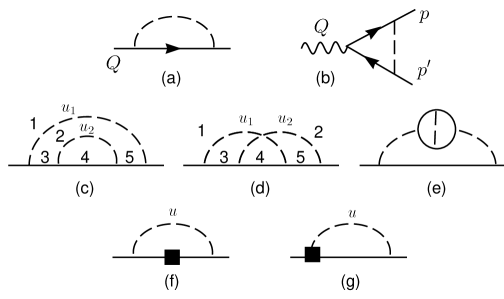
Figure 3: Self-energy diagrams at next-to-leading order in $1/N_{f}$ ((c)–(e)). (a) and (b) show the non-vanishing subgraphs for diagrams (c), (d). (f) and (g) show the reduced diagrams with insertion of a polynomial in external momenta of the contracted subgraphs in (c) and (d).

The self-energy requires renormalization beyond renormalization of the coupling. In general this requirement is translated into the necessity to subtract those singularities in the $u_{j}$ that give rise to a singularity at $u=0$ of the Borel transform. (Such a singularity prevents the calculation of coefficients $r_{n}$ of the perturbative expansion as derivatives of the Borel transform at $u=0$, see Sect. 2.1.) In the present case, the pole at $u=0$ is absent, because the logarithmic UV divergence of the one-loop self-energy cancels in Landau gauge. When fermion loops are inserted in the photon line, logarithmic overall divergences are present. In terms of the Borel transform their subtraction in a specified scheme amounts to subtracting an arbitrary function of $u$ with the only restriction that it does not have a pole at $u=0$. In the $\overline{\rm MS}$ scheme this function is entire [11] and does not introduce new singularities at any $u$. In general, it is quite non-trivial to determine this function in a given renormalization scheme (for a single chain see [11], appendix A). We do not discuss this point further, since our main interest concerns physical quantities. In this case all subtractions necessary for UV finiteness are implicitly contained in the definition of the renormalized complete photon propagator.

Let us now turn to the diagrams c and d in Fig. 3. Each maximal forest contains two non-trivial elements, the entire graph $\Gamma$ and a one-loop subgraph $\gamma$. The contributions from most forests vanish, because the reduced graph $\Gamma/\gamma$ is a tadpole graph, for instance in case of $\gamma=\{1,2,4,5\}$ for diagram c. For diagram c only one non-vanishing forest remains, ${\cal F}=\{\{2,4\},\Gamma_{c}\}$, for diagram d we have $\{\{1,3,4\},\Gamma_{d}\}$ and the symmetric forest $\{\{2,4,5\},\Gamma_{d}\}$. The leading singularity has two singular factors: $1/(1-u)$ from $\Gamma/\gamma$ and $1/(1-u_{j})$ ($j=1,2$) or $1/u_{j}$ from $\gamma$. Thus the leading singularity at $u=1$ arises from the points $\underline{u}_{0}=(1,0)$ and $\underline{u}_{0}=(0,1)$ in regularization parameter space.

We consider first diagram c and the vicinity of $(0,1)$. If we denote the momentum of lines 2 and 5 by $Q-k_{1}$, the pole part of $\gamma=\{2,4\}$ is given by the second line of eq. (3.3) with $u$ replaced by $u_{2}$ and $Q$ by $Q-k_{1}$. The insertion of the polynomial in $Q-k_{1}$ associated with the contraction of $\gamma$ into the reduced graph is shown in Fig. 3f. The corresponding Feynman integral (up to constants that can be read off eq. (3.3)) is given by

$$\frac{1}{1-u_{2}}\int\frac{{\mbox{d}}^{4}k_{1}}{(2\pi)^{4}}\frac{\gamma_{\mu}\,(\!\not\!Q-\!\not\!k_{1})(Q-k_{1})^{2}(\!\not\!Q-\!\not\!k_{1})(\!\not\!Q-\!\not\!k_{1})\gamma_{\nu}}{(Q-k_{1})^{4}}\frac{1}{(k_{1}^{2})^{1-u}}\left(g_{\mu\nu}-\frac{k_{\mu}k_{\nu}}{k^{2}}\right)\,.$$ (3.4)

The denominator in $Q-k_{1}$ is cancelled and the integral vanishes. In the vicinity of the other point, $u_{1}$=1, $u_{2}=0$, the potential pole $1/u_{2}$ is absent due to finiteness of the one-loop self-energy in Landau gauge as noted above. Thus diagram c does not contribute at all to the leading singularity. Note that according to eq. (3.2) and the appendix, the regularization parameter associated with the photon line of the reduced diagram is $u=u_{1}+u_{2}$, rather than $u_{1}$. In other words, the reduced diagram inherits the $u$-parameters from the contracted subgraph, here $u_{2}$. The reason for this is that the singularities in $\underline{u}$ from an element $\gamma_{+}\in{\cal F}$ (in the present example $\gamma_{+}=\Gamma$) are determined by $u(\gamma_{+})$, rather than $u(\gamma_{+}/\gamma)$, see Sect. 2.2. A less formal argument comes from doing the subgraph $\gamma$ exactly. Simply by dimensional reasons the Borel transform is proportional to $(\mu^{2}/(Q-k_{1})^{2})^{-u_{2}}$, so that the parameter $u_{2}$ is attached to the fermion line of the reduced graph. The singularities of the reduced graph arise in turn from the integration region $k_{1}\gg Q$, so that we may neglect $Q$ in this expression and attach the parameter $u_{2}$ to the photon line, where it combines with $u_{1}$ to $u$. This statement is true in general (see the appendix): In calculating the leading singularity, the $u$-parameters inherited from the contracted subgraph can be attached to an arbitrary line of the reduced graph.

Turning to diagram d, consider the forest $\{\{1,3,4\},\Gamma_{d}\}$. Again we have to analyze the points $\underline{u}_{0}=(1,0)$ and $\underline{u}_{0}=(0,1)$. The second one does not contribute two singular factors, since the one-loop vertex subgraph $\{1,3,4\}$ shown in Fig. 3b is UV finite in Landau gauge, so that no singularity $1/u_{1}$ occurs. In the vicinity of the first point we require the singularity of the vertex subgraph at $u_{1}=1$. With the momentum assignments of Fig. 3b we find

$$\int\frac{{\mbox{d}}^{4}k}{(2\pi)^{4}}\frac{\gamma_{\rho}(\!\not\!p-\!\not\!k)\gamma_{\nu}(\!\not\!p^{\prime}-\!\not\!k)\gamma_{\sigma}}{(p-k)^{2}(p^{\prime}-k)^{2}(k^{2})^{1-u_{1}}}\left(g_{\mu\nu}-\frac{k_{\mu}k_{\nu}}{k^{2}}\right)$$

$$\stackrel{{\scriptstyle u_{1}\rightarrow 1}}{{=}}\,\frac{i}{16\pi^{2}}\frac{1}{1-u_{1}}\left[-\frac{2}{3}(Q^{2}\gamma_{\mu}-\!\not\!QQ_{\mu})+\frac{1}{2}\left(\left(p^{2}+{p^{\prime}}^{2}\right)\gamma_{\mu}+\!\not\!p\gamma_{\mu}\!\not\!p^{\prime}\right)\right]\,,$$ (3.5)

where $Q=p^{\prime}-p$ is the momentum of the external photon. Note that the terms not containing $Q$ in the second line vanish on-shell and in the Lorentz structure of the terms containing $Q$ one recognizes the Feynman rule for insertion of the operator $\bar{\psi}\gamma_{\nu}\psi\partial_{\mu}F^{\mu\nu}$.

In order to calculate the pole parts of one-loop integrals like the vertex above, one should use the fact that the poles of interest are of ultraviolet origin, that is from the region of integration, where $k$ is much larger than all external momenta. Therefore we can expand the denominator in $p/k$ and $p^{\prime}/k$. The IR divergences that arise in this way can be regularized by a cut-off $|k|>\mu$ or in any other convenient way. Lorentz invariance then allows us to drop all terms with an odd number of $k$’s in the numerator and to simplify the numerator by relations such as $k_{\rho}k_{\sigma}\rightarrow g_{\rho\sigma}/4$ and its generalizations to more factors of $k$. If the original integral was logarithmically UV divergent, the result is expressed as the sum

$$\sum_{n=0}{\cal P}_{n}(\underline{q})\,(-16i\pi^{2})\int\limits_{|k|>\mu}\frac{{\mbox{d}}^{4}k}{(2\pi)^{4}}\frac{1}{(k^{2})^{2+n-u(\gamma)}}\,,$$ (3.6)

where ${\cal P}_{n}(\underline{q})$ is a polynomial of degree $n$ in the external momenta. The $k$-integral gives a pure pole, so that ${\cal P}_{n}(\underline{q})$ can be identified with the residue in eq. (3.2) that is to be inserted into the reduced graph. For the fermion-photon vertex ${\cal P}_{0}(\underline{q})$ vanishes and for ${\cal P}_{1}(\underline{q})$ we obtain eq. (3.2). Notice that the pole at $u=n$ is related to the term ${\mbox{d}}^{4}k/(k^{2})^{2+n}$ in the expansion of the integrand. The relation to Taylor operators is clarified further in the appendix.

The remainder of the calculation is straightforward. Eq. (3.2) is inserted into the reduced graph shown in Fig. 3g and the singular part of the reduced graph is extracted in the same way as before. Adding the contribution from the symmetric forest, we arrive at

$$G_{\Gamma_{d}}(Q;u_{1},u_{2})=\frac{i}{(4\pi)^{2}}\,Q^{2}\not\!Q\,\left(-\frac{1}{3}\right)\frac{1}{1-u_{1}-u_{2}}\left[\frac{1}{1-u_{1}}+\frac{1}{1-u_{2}}\right]\,.$$ (3.7)

After integration over $u_{1}$ and $u_{2}$ according to eq. (2.13), the final result for the leading singularity at $u=1$ from the two-chain diagrams c and d is

$$B_{\bar{\Gamma}_{c}}[\Sigma](u)+B_{\bar{\Gamma}_{d}}[\Sigma](u)\stackrel{{\scriptstyle u\rightarrow 1}}{{=}}\frac{i}{4\pi}\left(-\frac{Q^{2}}{\mu^{2}}e^{C}\right)\not\!Q\,\frac{1}{2}\frac{1}{1-u}\,\frac{1}{N_{f}}\left[\ln(1-u)+{\cal O}(1)\right]\,,$$ (3.8)

which has to be compared with the leading order contribution, eq. (3.3). (The factor $1/N_{f}$ originates from $1/\beta_{0}$ in eq. (2.13).) In this case we find $\beta_{0}^{n}n!\,\ln n$ for large $n$ with a logarithmic enhancement as compared to the leading order. The ${\cal O}(1)$ contribution in brackets will be found in Sect. 3.4. This concludes the illustration of the general method of extracting the leading singularity. The algebraically more extensive case of the vertex and vacuum polarization is treated in Sect. 4.

3.3 Next-to-leading singularity and IR rearrangement

At this point it is helpful to refer again to the large-order behaviour of perturbative expansions, eq. (1.2). Within the expansion in the number of chains, we write

$$K=K^{[1]}\,(1+\delta K^{[2]}+\ldots),\qquad b=b^{[1]}+b^{[2]}+\ldots\,,$$ (3.9)

where $\delta K^{[N]}$, $b^{[N]}$ denote contributions from $N$ chains. Since we expand in chains before taking the large-$n$ limit, eq. (1.2) must be written as

$$r_{n}=K^{[1]}\,\beta_{0}^{n}\,n!\,n^{b^{[1]}}\left(1+\left\{b^{[2]}\ln n+\delta K^{[2]}\right\}+\ldots\right)\left[1+{\cal{O}}\!\left(\frac{1}{n}\right)\right]\,,$$ (3.10)

where the ellipses represent terms like ${b^{[2]}}^{2}\ln^{2}n$ etc. from diagrams with three and more chains. Close to $u=1$, the corresponding Borel transform eq. (2.6) is

$$B[G](\underline{q};u) = \frac{K^{[1]}\Gamma(1+b^{[1]})}{(1-u)^{1+b^{[1]}}}\left(1+\left\{-b^{[2]}\left(\ln(1-u)-\psi(1+b^{[1]})\right)+\delta K^{[2]}\right\}\ldots\right)$$ (3.11)

$$\times\left[1+{\cal O}\left((1-u)\ln^{k}(1-u)\right)\right]\,,$$

where $\psi(x)$ is Euler’s $\psi$-function. From this expression we deduce that $b^{[2]}$ can be read off from the leading singularities of diagrams with two chains, such as those considered in the previous subsection. On the other hand to obtain the first correction $\delta K^{[2]}$ to the normalization, we require also some terms with only one singular factor. This can be either $1/(1-u_{1}-u_{2})$ or $1/(1-u_{j})$ ($u_{j}=1,2$). After integration over $u_{1}$, $u_{2}$, the second type produces a singularity $\ln(1-u)$ and contributes only to $1/n$-corrections in eq. (3.10). Thus, we consider only singular factors of type $1/(1-u)$.

This distinction is important both as far as the physical origin of the singularity is concerned as well as its extraction. Recall that, for example for the contribution from Fig. 3d to the self-energy, the leading singularity (two singular factors) comes from the loop momentum regions

$$Q\ll k_{1}\ll k_{2}\qquad Q\ll k_{2}\ll k_{1}\,.$$ (3.12)

To obtain at least one singular factor, we must consider the regions

$$Q\ll k_{1}\sim k_{2}\,,$$

$$Q\sim k_{1}\ll k_{2}\qquad Q\sim k_{2}\ll k_{1}\,.$$ (3.13)

Only in the first case we obtain $1/(1-u)$, because both virtual photons have momentum larger than the external momentum $Q$, so that the large-momentum part of the diagram contains all available $u$-parameters. Moreover, because of this, the residue of the pole is polynomial in the external momentum. On the other hand, the regions listed in the second line lead to singularities $1/(1-u_{j})$. The residue is no longer ‘local’ (polynomial in external momenta), but contains $\ln(Q^{2}/\mu^{2})$. A simple way to see this is to note that by dimensional reasons the Borel transform for diagram d is proportional to $\!\not\!Q\,(Q^{2}/\mu^{2})^{u}$. This implies that the leading singularity at $u=1$ in fact arises in the combination

$$\!\not\!Q\,Q^{2}\,\frac{1}{1-u_{j}}\left[\frac{1}{1-u}-\ln\frac{Q^{2}}{\mu^{2}}\right]\,,$$ (3.14)

so that the coefficient of the logarithm is related to the residue for the leading singularity. One may compare this with the $1/\epsilon^{2}$ and $(1/\epsilon)\ln(Q^{2}/\mu^{2})$ poles for a dimensionally regularized two-loop integral before the subtraction of subdivergences is taken into account.

We also see that if explicit renormalization (in the usual sense) is needed as in case of the self-energy, the arbitrariness in choosing finite subtractions affects only the residues of $1/(1-u_{j})$. Indeed, the effect of such a subtraction is described by (taking $j=2$, so that the logarithmic UV divergence occurs in the subgraph with photon line regularized by $u_{1}$)

$$\frac{1}{1-u}\frac{a}{u_{1}}-\frac{1}{1-u_{2}}\left[\frac{a}{u_{1}}+G(u_{1})\right]=\frac{a}{(1-u)(1-u_{2})}-\frac{G(u_{1})}{1-u_{2}}\,,$$ (3.15)

where $G(u_{1})$ has no pole at $u_{1}=0$, but is arbitrary otherwise. Recall that $a$ is in fact zero for the self-energy (in Landau gauge). We therefore conclude that the terms that contribute to $\delta K^{[2]}$ are local and do not depend on the renormalization scheme.

The fact that the residues of the singular factors that contribute to the overall normalization of renormalon divergence are polynomial in the external momenta allows us to use the method of IR rearrangement [15, 16] (see also [25] for a review) which was originally developed for and successfully applied to renormalization group calculations. In its original form, the method is based on polynomial dependence of UV counterterms on momenta and masses. It consists of the following two steps: (a) Differentiation in external momenta and internal masses. The problem thereby reduces to the calculation of zero-degree polynomials. (b) Putting to zero all the internal masses and external momenta except one. Usually, at step b one puts to zero all the momenta and masses and chooses a new momentum that flows through the diagram in some appropriate way. The goal is to make this choice in such a way that the diagram becomes calculable. In simple cases the problem reduces to calculation of the pole part of primitively divergent propagator-type integrals or vacuum integrals with one non-zero mass. The application in the present context is illustrated in Sect. 3.4.

The arguments presented above can easily be generalized to the contribution $\delta K^{[N]}$ to the normalization $K$ from $N$ chains. For such a contribution we need at least one singular factor of type $1/(1-u)$, (with $u=u_{1}+\ldots+u_{N}$). Although no ordering of loop momenta is required, all loop momenta $k_{i}$ have to be much larger than the external momenta $\underline{q}$ in order to get such a singular factor. Therefore the residue of these terms remains local for any $N$. Similarly, if UV renormalization is necessary, the arbitrariness in choosing finite subtractions affects the singularity of the Borel transform only at the level of $\ln^{k}(1-u)$ (where typically $k<N$) and therefore modifies only the $1/n$-corrections to the asymptotic behaviour in eq. (3.10). A scheme-dependence enters the overall normalization only through the subtraction constant $C$ for the fermion loop [26], see eq. (2.10). With the help of IR rearrangement, the calculation of $K$ to an arbitrary order in the expansion in chains reduces to extracting pole parts of primitively divergent propagator-type integrals or vacuum integrals with one non-zero mass.

Note that IR rearrangement can be applied also to the calculation of $1/n$ corrections to the asymptotic behaviour. Because of the logarithms in external momenta that enter in this place, one must apply explicit subtractions in subgraphs, which remove these logarithms. Since the combinatorial structure of eq. (2.23) is completely analogous to the one that arises in the context of usual renormalization, the combinatorial structure of the subtraction operator is equally simple. We will return to this point in Sect. 5.

3.4 Self-energy: The next-to-leading singularity

In this subsection we illustrate the calculation of $\delta K^{[2]}$ and the use of IR rearrangement for this purpose by continuing with the fermion self-energy. When $\Gamma=\Gamma_{c},\Gamma_{d}$ as shown in Fig. 3c and d, we have for the integral in eq. (2.13) the following asymptotic behaviour at $u\to 1$:

$$\int_{0}^{u}{\mbox{d}}u^{\prime}\,G_{\Gamma}(Q;u^{\prime},u-u^{\prime})\stackrel{{\scriptstyle u\rightarrow 1}}{{=}}\frac{1}{1-u}\left[a_{1}(Q)\ln(1-u)+a_{2}(Q)+{\cal O}\left((1-u)\ln(1-u)\right)\right]\,,$$ (3.16)

where $a_{i}$ are proportional to $\not\!QQ^{2}$ with no logarithm in $Q^{2}/\mu^{2}$ as explained in Sect. 3.3. ($a_{1}(Q)$ is given in eq. (3.8).) According to eq. (2.23), the function $G_{\Gamma}(u_{1},u_{2})$ can be represented as

$$G_{\Gamma}(u_{1},u_{2})=\frac{1}{1-u_{1}-u_{2}}\left[\frac{g_{1}(u_{1},u_{2})}{1-u_{1}}+\frac{g_{2}(u_{1},u_{2})}{1-u_{2}}\right]\equiv\frac{h(u_{1},u_{2})}{(1-u_{1}-u_{2})(1-u_{1})(1-u_{2})}\,.$$ (3.17)

Now we apply the following proposition: If $f(u^{\prime})$ is analytic at $0\leq u^{\prime}\leq 1$ then

$$\int_{0}^{u}{\mbox{d}}u^{\prime}\frac{f(u^{\prime})}{(1-u^{\prime})(1-u+u^{\prime})}\stackrel{{\scriptstyle u\rightarrow 1}}{{=}}-[f(0)+f(1)]\ln(1-u)$$ (3.18)

when $u\to 1$. As a result we have

$$\int_{0}^{u}{\mbox{d}}u_{1}{\mbox{d}}u_{2}\,\delta(u_{1}+u_{2}-u)\frac{h(u_{1},u_{2})}{(1-u_{1}-u_{2})(1-u_{1})(1-u_{2})}$$

$$\hskip 28.45274pt=\,-[h(1,0)+h(0,1)]\,\frac{\ln(1-u)}{1-u}+\frac{1}{1-u}\int_{0}^{1}{\mbox{d}}u^{\prime}\overline{h}(u^{\prime},1-u^{\prime}),$$ (3.19)

when $u\to 1$. Here

$$\overline{h}(u^{\prime},1-u^{\prime}) = \frac{h(u^{\prime},1-u^{\prime})}{u^{\prime}(1-u^{\prime})}-\frac{h(1,0)}{1-u^{\prime}}-\frac{h(0,1)}{u^{\prime}}$$ (3.20)

$$= \frac{g_{1}(u^{\prime},1-u^{\prime})-g_{1}(1,0)}{1-u^{\prime}}+\frac{g_{2}(u^{\prime},1-u^{\prime})-g_{2}(0,1)}{u^{\prime}}\,.$$

Define $b_{1}=g_{1}(1,0)$ and $b_{2}=g_{2}(0,1)$, so that the leading singularity is determined by

$$G_{\Gamma}(Q;u_{1},u_{2})=\frac{1}{1-u_{1}-u_{2}}\frac{b_{1}}{1-u_{1}}\quad{\rm near}\quad u_{1}=1,u_{2}=0\,,$$

$$G_{\Gamma}(Q;u_{1},u_{2})=\frac{1}{1-u_{1}-u_{2}}\frac{b_{2}}{1-u_{2}}\quad{\rm near}\quad u_{1}=0,u_{2}=1\,.$$ (3.21)

Then the coefficients that enter eq. (3.16) are expressed as

$$a_{1} = -b_{1}-b_{2},$$

$$a_{2} = \int_{0}^{1}{\mbox{d}}u^{\prime}\left\{\mbox{res}_{u-1}G_{\Gamma}(Q;u^{\prime},u-u^{\prime})-\frac{b_{1}}{1-u^{\prime}}-\frac{b_{2}}{u^{\prime}}\right\}.$$ (3.22)

Generally speaking, one can directly use eq. (3.4) for calculation. This is indeed possible for the rainbow diagram of Fig. 3c, which can be computed exactly for arbitrary $u_{1}$ and $u_{2}$. After a straightforward calculation, we get

$$a_{1} = 0\quad\mbox{(see Sect.~{}3.2)}$$

$$\overline{h}(u^{\prime},1-u^{\prime}) = \frac{i}{(4\pi)^{2}}\,Q^{2}\!\not\!Q\,\left(-\frac{3}{2}\right)\frac{1-u^{\prime}}{2+u^{\prime}}\,.$$ (3.23)

Integration according to eq. (3.4) and reinstating the factors from eq. (2.13) yields

$$B_{\bar{\Gamma}_{c}}[\Sigma](u)\stackrel{{\scriptstyle u\rightarrow 1}}{{=}}\frac{i}{4\pi}\left(-\frac{Q^{2}}{\mu^{2}}e^{C}\right)\not\!Q\,\frac{1}{2}\frac{1}{1-u}\,\frac{1}{N_{f}}\left[\frac{27}{4}\ln\frac{2}{3}+\frac{9}{4}\right]\,.$$ (3.24)

In most cases, however, the analytically regularized Feynman integral is hardly calculable for arbitrary values of $u_{1}$ and $u_{2}$. This is true in particular already for diagram d in Fig. 3. In this situation one first calculates coefficients $b_{1}$ and $b_{2}$ (and if necessary also the coefficients of terms $1/((1-u)u_{j})$) with the help of general statements regarding the leading singularity, and then the function that enters the integrand of eq. (3.4) using IR rearrangement. To apply IR rearrangement to diagram d we use the fact that the coefficients $a_{i}$ are polynomials in $Q$, in this case $\not\!QQ^{2}$. Thus we differentiate three times. Since $\partial_{Q}^{2}\!\not\!\partial_{Q}\not\!QQ^{2}=48$, the substitution

$$G_{\Gamma}(Q;u^{\prime},u-u^{\prime})\longrightarrow\,\not\!QQ^{2}\,\frac{1}{48}\partial_{Q}^{2}\!\not\!\partial_{Q}G_{\Gamma}(Q;u^{\prime},u-u^{\prime})$$ (3.25)

leaves the coefficient $a_{2}(Q)$ unchanged. To reduce the number of terms that arise in the process of differentiation, we route the external momentum $Q$ through the lines 1 and 5 in Fig. 3d, so that the corresponding momenta are $Q-k_{1}$ and $Q-k_{2}$, respectively. The threefold differentiation of the product of photon propagator and fermion propagator gives rise to six new diagrams $\Gamma_{i}$ with the same topology as the original diagram but with propagators differentiated in a special way. The residue

$$\mbox{res}_{u-1}G_{\Gamma_{i}}(Q;u^{\prime},u-u^{\prime})$$ (3.26)

for each diagram is now a number independent of the external momentum $Q$. The second step in the IR rearrangement is to apply the equation

$$\mbox{res}_{u-1}G_{\Gamma_{i}}(Q;u^{\prime},u-u^{\prime})=\mbox{res}_{u-1}G^{\prime}_{\Gamma_{i}}(p;u^{\prime},u-u^{\prime})\,.$$ (3.27)

The meaning of this equation is as follows: Instead of the initial external momentum $Q$, one introduces a new external momentum $p$ which flows through the diagram in some appropriate way. In our example diagram d (and its descendents $\Gamma_{i}$) we choose $p$ to flow through line 5 (so that the vertex to which lines 1, 4, 5 are attached becomes external). Due to this choice of external momentum the ‘new’ diagram $G^{\prime}_{\Gamma_{i}}(p;u^{\prime},u-u^{\prime})$ becomes explicitly calculable by consecutive application of one-loop integrations.

The extensive algebra connected with numerators of integrals after differentiation can be done with the help of REDUCE [27]. A generic integral has the form

$$\int\frac{{\mbox{d}}^{4}k_{1}}{(2\pi)^{4}}\frac{{\mbox{d}}^{4}k_{2}}{(2\pi)^{2}}\frac{N(k_{1},k_{2},p)}{(k_{1}^{2})^{a}((k_{1}-k_{2})^{2})^{b}(k_{2}^{2})^{c}((p-k_{2})^{2})^{d}}\,.$$ (3.28)

We can take the $k_{1}$-integral. Since the remaining $k_{2}$ satisfies $k_{2}\gg p$ to obtain a singularity $1/(1-u)$, we can then extract the pole factor from the $k_{2}$-integral by expansion in the external momentum as in Sect. 3.2. Summing over all six contributions from differentiation, we obtain

$$a_{1} = \frac{i}{(4\pi)^{2}}\,Q^{2}\!\not\!Q\left(-\frac{2}{3}\right)\quad\mbox{(see Sect.~{}3.2)}$$

$$\overline{h}(u^{\prime},1-u^{\prime}) = \frac{i}{(4\pi)^{2}}\,Q^{2}\!\not\!Q\,\frac{1}{3}\left[\frac{3}{2}-\frac{1}{2+u^{\prime}}+\frac{1}{1+u^{\prime}}+\frac{1}{2-u^{\prime}}-\frac{1}{3-u^{\prime}}\right]\,.$$ (3.29)

Integration according to eq. (3.4) and reinstating the factors from eq. (2.13) yields

$$B_{\bar{\Gamma}_{d}}[\Sigma](u)\stackrel{{\scriptstyle u\rightarrow 1}}{{=}}\frac{i}{4\pi}\left(-\frac{Q^{2}}{\mu^{2}}e^{C}\right)\not\!Q\,\frac{1}{2}\frac{1}{1-u}\,\frac{1}{N_{f}}\left[\ln(1-u)+2\ln 2-\ln 3+\frac{3}{4}\right]\,.$$ (3.30)

When combined with eq. (3.24), this results in

$$\delta K^{[2]}_{c+d}=\frac{1}{4}\left(35\ln 2-31\ln 3+12\right)\,.$$ (3.31)

3.5 Self-energy: Propagator corrections and summary

To complete the calculation of all contributions at subleading order in $1/N_{f}$ (for the $N_{f}$-counting one rescales $a=\alpha N_{f}$) we have to analyze diagram e in Fig. 3 (plus the self-energy type contributions to the vacuum polarization insertion, not shown in the figure). This diagram is treated differently from c and d, because it appears as the first correction to approximating the complete photon propagator in eq. (2.11) by a chain, the first term on the right hand side of eq. (2.11). Corrections of this type have been considered previously in [9, 28]. To include the second term in eq. (2.11), we write, as in [28],

$$F_{\rm reg}(u)=F(u)+\frac{1}{u}\,,\qquad G_{\rm reg}(u)=G(u)+\frac{1}{u}\,,$$ (3.32)

where $F(u)$ is given in eq. (2.12) and $F_{\rm reg}(u)$ and $G_{\rm reg}(u)$ are finite at $u=0$. When the second term on the right hand side of eq. (2.11) is inserted for the single complete photon propagator in eq. (2.9), we obtain

$$B_{\bar{\Gamma}_{e}}[\Sigma](u) = \frac{\beta_{1}}{\beta_{0}^{2}}\int\limits_{0}^{u}\frac{dv\,v}{u-v}\left(B_{\bar{\Gamma}_{a}}[\Sigma](u)-B_{\bar{\Gamma}_{a}}[\Sigma](v)\right)$$ (3.33)

$$-\,\frac{\beta_{1}}{\beta_{0}^{2}}\int\limits_{0}^{u}dv\,v\left(B_{\bar{\Gamma}_{a}}[\Sigma](u)\,F_{\rm reg}(u-v)-B_{\bar{\Gamma}_{a}}[\Sigma](v)\,G_{\rm reg}(u-v)\right)\,,$$

where $B_{\bar{\Gamma}_{a}}[\Sigma](u)$ is the leading order contribution given in eq. (3.3). The vacuum polarization insertion requires renormalization and the function $G(u)$ takes into account the arbitrariness of finite subtractions, that is, the arbitrariness in defining the renormalized coupling $\alpha=\alpha(\mu)$. We evaluate eq. (3.33) in two schemes: The $\overline{\rm MS}$ scheme, in which case $G_{\rm reg}(u)$ is an entire function [17, 28], and the so-called MOM scheme, where the renormalized coupling is defined by

$$\alpha_{\rm MOM}(\mu)=\frac{\alpha_{R}(\mu^{\prime})}{1+\Pi_{R}(\mu/\mu^{\prime},\mu^{\prime})}\,,$$ (3.34)

where $R$ denotes any renormalization scheme or bare quantities. In this scheme we have $F(u)=G(u)$ [17] and eq. (3.33) takes the particularly simple form

$$B_{\bar{\Gamma}_{e}}^{\rm MOM}[\Sigma](u)=\frac{\beta_{1}}{\beta_{0}^{2}}\int\limits_{0}^{u}dv\,v\left[\frac{1}{u-v}-F_{\rm reg}(u-v)\right]\left(B_{\bar{\Gamma}_{a}}[\Sigma](u)-B_{\bar{\Gamma}_{a}}[\Sigma](v)\right)\,.$$ (3.35)

Contrary to the $\overline{\rm MS}$ scheme, the finite subtractions are themselves factorially divergent in this scheme.

The right hand side of the first line of eq. (3.33) is easily evaluated as $u\to 1$, given that $B_{\bar{\Gamma}_{a}}[\Sigma](v)\sim 1/(1-v)$ close to $v=1$. We get

$$\frac{\beta_{1}}{\beta_{0}^{2}}\int\limits_{0}^{u}\frac{dv\,v}{u-v}\left(B_{\bar{\Gamma}_{a}}[\Sigma](u)-B_{\bar{\Gamma}_{a}}[\Sigma](v)\right)\stackrel{{\scriptstyle u\to 1}}{{=}}-\frac{\beta_{1}}{\beta_{0}^{2}}\,B_{\bar{\Gamma}_{a}}[\Sigma](u)\left(\ln(1-u)+1\right)$$ (3.36)

up to ${\cal O}((1-u)\ln(1-u))$ terms. To evaluate the second line in eq. (3.33), we note first that we can drop the contribution from $G_{\rm reg}$ as long as we are not interested in singularities weaker than $1/(1-u)$. In the $\overline{\rm MS}$ scheme, this follows from $G_{\rm reg}(u)$ being entire, so that one gets only a $\ln(1-u)$-singularity from $v$ close to one. In the MOM scheme, we also observe singular behaviour when $v$ is close to zero, but since $B_{\bar{\Gamma}_{a}}[\Sigma](v)$ is finite as $v\to 0$, one gets again only $\ln(1-u)$. Therefore, to the present accuracy, the results in the $\overline{\rm MS}$ and MOM scheme are the same. Next we separate the double pole of $F_{\rm reg}(u)$ at $u=1$, since it gives rise to a logarithmic singularity of the $v$-integral at $u=1$. In the remaining terms we can set $u=1$. Adding the result from the previous equation we obtain

$$B_{\bar{\Gamma}_{e}}[\Sigma](u)\stackrel{{\scriptstyle u\to 1}}{{=}}B_{\bar{\Gamma}_{a}}[\Sigma](u)\left[\left(-\frac{\beta_{1}}{\beta_{0}^{2}}-\frac{1}{N_{f}}\right)\ln(1-u)+\frac{1}{N_{f}}\,\delta K_{\rm prop}\right]\,,$$ (3.37)

where

$$\delta K_{\rm prop} = -\frac{2}{3}+\frac{233}{12}\ln 2-\frac{157}{12}\ln 3$$ (3.38)

$$\,-\,24\sum_{k=3}^{\infty}\frac{(-1)^{k}k}{(k^{2}-1)^{2}}\left\{\frac{1}{2k^{2}}+\frac{1}{2}\ln\frac{k^{2}-1}{k^{2}-4}+\frac{3k^{2}-1}{k^{3}}\left[\mbox{arctan}\frac{1}{k}-\mbox{arctan}\frac{2}{k}\right]\right\}$$

$$= -1.7266\ldots\,.$$

Recall that $\beta_{1}/\beta_{0}^{2}=9/(4N_{f})={\cal O}(1/N_{f})$. We can now combine eqs. (3.24), (3.30) and (3.37) to obtain the final result for the self-energy to subleading order in $1/N_{f}$:

$$B[\Sigma](u) \stackrel{{\scriptstyle u\rightarrow 1}}{{=}} \frac{i}{4\pi}\left(-\frac{Q^{2}}{\mu^{2}}e^{C}\right)\not\!Q\,\frac{1}{2}\frac{1}{1-u}\,\Bigg{[}1-\frac{\beta_{1}}{\beta_{0}^{2}}\ln(1-u)+\frac{1}{N_{f}}\left(\delta K^{[2]}_{c+d}+\delta K_{\rm prop}\right)$$ (3.39)

$$\vspace*{1cm}+\,{\cal O}\!\left((1-u)\ln(1-u),\frac{1}{N_{f}^{2}}\right)\Bigg{]}\,,$$

with $\delta K^{[2]}_{c+d}$ given in eq. (3.31). By comparison of eq. (3.11) with eq. (3.10), this result can be translated into the large-order behaviour of the self-energy. Notice that there is a cancellation of $\ln(1-u)/(1-u)$ terms between diagrams d and e of Fig. 3 and the only remaining logarithmic enhancement is proportional to $\beta_{1}/\beta_{0}^{2}$. This remaining term can be traced to eq. (3.36) and then further to the coefficient of the pole of $F(u)$ at $u=0$. It is therefore unambiguously identified as the expected correction to $b$ in eq. (1.2) due to two-loop evolution of the coupling (see Sect. 5).

The cancellation between vertex and propagator corrections is of general nature and recurs in further examples in Sect. 4. It can be phrased as a cancellation between the two subgraphs shown in Fig. 4. Note that these subgraphs are of the same order in $1/N_{f}$ and for any diagram that contains the left subgraph there is a diagram that contains the right one and vice versa. Assume that these diagrams have $N$ and $N+1$ chains respectively. The contraction of the left vertex subgraph gives $c/(1-u_{N})$ with some constant $c$. Now consider the other subgraph. Contraction of the vertex subgraph in the inner box gives $c/(1-u_{N+1})$ with the same constant $c$ when $u_{N+1}$ is close to one. The subsequent contraction of the second box turns the simple pole into a double pole. If one takes into account all factors, including the different power of $\beta_{0}$ in eq. (2.13), one finds that the coefficient of the double pole is $(-i)c$. After this contraction, the lower chain carries regularization parameter $u_{N}+u_{N+1}$. A factor $(-i)$ from one photon propagator is obtained from joining the two chains into one (this can be done, since both have the same momentum). One can then make use of the $\delta$-function constraint in eq. (2.13). From the left diagram we get simply

Figure 4: Cancellation of leading singularities between vertex and propagator corrections. Since these graphs should be inserted as subgraphs, the external photon lines are drawn as chains.

$$\frac{c}{1-(u-u_{1}\ldots-u_{N-1})}$$ (3.40)

and from the right

$$\int\limits_{0}^{u-u_{1}-\ldots-u_{N-1}}\!\!\!du_{N}\frac{(-c)}{(1-(u-u_{1}\ldots-u_{N-1}-u_{N}))^{2}}\,.$$ (3.41)

Both contributions cancel each other up to non-singular terms. As a result the leading singularity drops out in the sum of the two diagrams that contain the graphs of Fig. 4 as subgraphs. This cancellation does not apply to the next-to-leading singularity of the diagrams.

Finally we note that eq. (3.33) is universal and can be used for any Green function with the obvious replacement for the corresponding leading order Borel transform.

4 Vertex function and vacuum polarization

In this section we turn to the classical example of the photon vacuum polarization. For reasons that will become clear it is useful to consider first the fermion-photon vertex function. We restrict ourselves to the leading singularity at $u=1$.

The photon vacuum polarization is gauge-independent. One can introduce a gauge parameter $\xi$, so that the Lorentz structure in eq. (2.15) takes the familiar form for covariant gauges. The result must be independent of $\xi$. In particular, one can take Feynman gauge and considerably simplify the algebra connected with numerators. The price to pay for this simplification is the presence of singular factors like $1/((1-u)u_{j})$ in individual diagrams, which are absent in Landau gauge, because the one-loop self-energy and vertex function are separately UV finite in this gauge. To render each diagram separately finite, one would have to add the usual counterterms. In practice we do not have to bother about these subtractions, since we know that all such singular factors must cancel in the final result. We have done the calculation for the vacuum polarization in an arbitrary covariant gauge and verified independence of $\xi$ explicitly. Gauge-dependent intermediate expressions that follow below are given in Landau gauge, as before.

4.1 Vertex function

The result for the leading order diagram with one chain, Fig. 3b, is obtained from eq. (3.2) after restoration of overall factors:

$$B_{\rm LO}[\Gamma](u)\stackrel{{\scriptstyle u\rightarrow 1}}{{=}}\,-\frac{1}{4\pi\mu^{2}}\,e^{C}\,\frac{1}{1-u}\left[-\frac{2}{3}(Q^{2}\gamma_{\mu}-\!\not\!QQ_{\mu})+\frac{1}{2}\left(\left(p^{2}+{p^{\prime}}^{2}\right)\gamma_{\mu}+\!\not\!p\gamma_{\mu}\!\not\!p^{\prime}\right)\right]\,.$$ (4.1)

The corresponding large-order behaviour is proportional to $\beta_{0}^{n}n!$. Recall that the coupling $(-ig)$ to the external photon is not included in the Borel transform.

4.1.1 Vertex diagrams with two chains

The diagrams with two chains are shown in Fig. 5. Any maximal forest of any of these diagrams has two 1PI elements, one of which is the diagram itself. According to eq. (3.2), the leading singularity arises from the combinations

$$\frac{1}{(1-u)^{2}}\,,\,\,\frac{1}{1-u}\frac{1}{1-u_{j}}\,,\,\,\frac{1}{1-u}\frac{1}{u_{j}}\,,$$ (4.2)

Figure 5: Vertex diagrams with two chains.

where the last combination is in fact absent. The first combination arises from ‘box’ subgraphs as discussed in Sect. 2.2. For each diagram, in each forest, there are three choices for the second 1PI element $\gamma\not=\Gamma$, which is a one-loop subgraph. For each of the 18 distinct combinations we have to consider the region $u(\gamma)=1$, where $u(\gamma)$ is the sum of $u$-parameters of the lines of the corresponding one-loop subgraph. The result is denoted by (Nx), where N=$1,\ldots,6$ for the six diagrams and x=a,b,c for the three possible one-loop subgraphs. Seven of the 18 combinations lead to insertions into reduced graphs that vanish. The remaining eleven ones are described as follows, according to their subgraph $\gamma$:

(1a): The ‘small’ vertex consisting of lines with momenta $k_{2},p^{\prime}-k_{1}-k_{2},p-k_{1}-k_{2}$.

(1b): The ‘box’ subgraph.

(2a): The subgraph consisting of lines with momenta $k_{2},p-k_{1}-k_{2},p^{\prime}-k_{1}-k_{2},p^{\prime}-k_{2}$.

(2b): The subgraph symmetric to (2a) with lines $k_{2},p-k_{1},p-k_{1}-k_{2},p^{\prime}-k_{1}-k_{2}$.

(2c): The ‘crossed box’ subgraph.

(3a): The subgraph with lines $k_{1},p-k_{1}-k_{2},p-k_{1},p^{\prime}-k_{1}$.

(3b): The vertex subgraph on the upper fermion leg.

(4a): The subgraph with lines $k_{1},p-k_{1},p^{\prime}-k_{1},p^{\prime}-k_{1}-k_{2}$, symmetric to (3a).

(4b): The vertex subgraph on the lower fermion leg.

(5a): The self-energy subgraph on the upper leg.

(6a): The self-energy subgraph on the lower leg.

In addition to subgraphs of self-energy [(5a),(6a)] and vertex type [(1a),(3b),(4b)], which have superficial degree of divergence $\omega(\gamma)=0$, we also encounter subgraphs with four external fermion legs [(1b),(2c)] and two fermion and two photon legs [(2a),(2b),(3a),(4a)] with $\omega(\gamma)=-2$.

Specifically, for the box-type subgraphs one obtains

$$\frac{i}{1-u}\frac{3\pi}{N_{f}}\left[\pm\frac{3}{4}\gamma_{\mu}\otimes\gamma^{\mu}-\frac{3}{2}\gamma_{\mu}\gamma_{5}\otimes\gamma^{\mu}\gamma_{5}\right]\,,$$ (4.3)

with the upper sign for (1b) and the lower sign for (2c). In the sum of both contributions only the structure $\gamma_{\mu}\gamma_{5}\otimes\gamma^{\mu}\gamma_{5}$ survives. Similar cancellations occur between other subgraphs and one should combine them before insertion in the reduced diagram. It is then straightforward to calculate the combinations

(I) $$=$$ (1a)

$$= -\frac{1}{12}\,(p^{2}+{p^{\prime}}^{2})\,\gamma_{\mu}+\frac{1}{3}\,(\!\not\!pp_{\mu}+\!\not\!p^{\prime}p^{\prime}_{\mu})-\frac{3}{2}\,(\!\not\!pp^{\prime}_{\mu}+\!\not\!p^{\prime}p_{\mu})+2p\cdot p^{\prime}\gamma_{\mu}+\!\not\!p\gamma_{\mu}\!\not\!p^{\prime}$$

(II) $$=$$ [(2a)+(3a)]+[(2b)+(4a)]

$$= \frac{1}{12}\,(p^{2}+{p^{\prime}}^{2})\,\gamma_{\mu}-\frac{1}{3}\,(\!\not\!pp_{\mu}+\!\not\!p^{\prime}p^{\prime}_{\mu})+\frac{1}{2}\,(\!\not\!pp^{\prime}_{\mu}+\!\not\!p^{\prime}p_{\mu})-2p\cdot p^{\prime}\gamma_{\mu}-\frac{1}{2}\,\!\not\!p\gamma_{\mu}\!\not\!p^{\prime}$$

(III) $$= \mbox{(3b)+(4b)}=\frac{8}{9}\,(Q^{2}\gamma_{\mu}-\!\not\!QQ_{\mu})$$

$$-\,\frac{3}{4}\,(p^{2}+{p^{\prime}}^{2})\,\gamma_{\mu}+\frac{1}{3}\,(\!\not\!pp_{\mu}+\!\not\!p^{\prime}p^{\prime}_{\mu})-\frac{1}{2}\,(\!\not\!pp^{\prime}_{\mu}+\!\not\!p^{\prime}p_{\mu})+2p\cdot p^{\prime}\gamma_{\mu}-\frac{1}{6}\!\not\!p\gamma_{\mu}\!\not\!p^{\prime}$$

(IV) $$=$$ (5a)+(6a)

$$= \frac{1}{12}\,(p^{2}+{p^{\prime}}^{2})\,\gamma_{\mu}-\frac{1}{3}\,(\!\not\!pp_{\mu}+\!\not\!p^{\prime}p^{\prime}_{\mu})+\frac{3}{2}\,(\!\not\!pp^{\prime}_{\mu}+\!\not\!p^{\prime}p_{\mu})-2p\cdot p^{\prime}\gamma_{\mu}-\!\not\!p\gamma_{\mu}\!\not\!p^{\prime}$$

(V) $$= \mbox{(1b)+(2c)}=2\,(Q^{2}\gamma_{\mu}-\!\not\!QQ_{\mu})$$

It is understood that each line is multiplied by $1/(16\pi^{2})$ and $1/(1-u)(1-u_{1})$ except for (V), where the latter factor is replaced by $1/(1-u)^{2}$. Note that (I) and (IV) cancel against each other. The other terms add to

$$G_{\bar{\Gamma}_{\rm(1)-(6)}}[\Gamma](u) \stackrel{{\scriptstyle\rm LS}}{{=}} -\frac{1}{12\pi^{2}}\Bigg{\{}\frac{1}{1-u}\frac{1}{1-u_{1}}\left[-\frac{2}{3}(Q^{2}\gamma_{\mu}-\!\not\!QQ_{\mu})+\frac{1}{2}\left(\left(p^{2}+{p^{\prime}}^{2}\right)\gamma_{\mu}+\!\not\!p\gamma_{\mu}\!\not\!p^{\prime}\right)\right]$$ (4.5)

$$\hskip 28.45274pt-\,\frac{3}{2}\,\frac{1}{(1-u)^{2}}\,(Q^{2}\gamma_{\mu}-\!\not\!QQ_{\mu})\Bigg{\}}\,.$$

The first line has exactly the same structure as the leading order result, eq. (4.1). After integration over the $u$-parameters, it leads to a singularity of the form $\ln(1-u)/(1-u)$,

$$B_{\rm LO}[\Gamma](u)\,\frac{1}{N_{f}}\ln(1-u)\,.$$ (4.6)

This is not the only contribution of this form, however. As in Sect. 3.5, eq. (3.37), the universal propagator corrections add

$$B_{\rm LO}[\Gamma](u)\,\left(-\frac{\beta_{1}}{\beta_{0}^{2}}-\frac{1}{N_{f}}\right)\ln(1-u)\,,$$ (4.7)

and by the same cancellation as for the self-energy only the term with $\beta_{1}/\beta_{0}^{2}$ is left.

Adding everything together, we find that, including diagrams with two chains and propagator corrections, eq. (4.1) is extended to

$$B_{\rm NLO}[\Gamma](u)\!\! \stackrel{{\scriptstyle u\rightarrow 1}}{{=}} \!\!-\frac{1}{4\pi\mu^{2}}\,e^{C}\Bigg{\{}\frac{1}{1-u}\left(1-\frac{\beta_{1}}{\beta_{0}^{2}}\ln(1-u)\right)\bigg{[}-\frac{2}{3}(Q^{2}\gamma_{\mu}-\!\not\!QQ_{\mu})+\frac{1}{2}\left(\Big{(}p^{2}+{p^{\prime}}^{2}\right)\gamma_{\mu}$$ (4.8)

$$\hskip 56.9055pt+\,\!\not\!p\gamma_{\mu}\!\not\!p^{\prime}\Big{)}\bigg{]}+\,\frac{3}{2N_{f}}\,\frac{1}{(1-u)^{2}}\,(Q^{2}\gamma_{\mu}-\!\not\!QQ_{\mu})\Bigg{\}}\,.$$

The first line has a similar structure as in case of the self-energy. The two-loop evolution of the coupling leads to a logarithmic enhancement in the large-order behaviour, $\beta_{0}^{n}n!\,\ln n$, while being formally of order $1/N_{f}$. The second line incorporates the contributions from box type subgraphs, which were absent for the self-energy (at the level of two chains). While this contribution starts at order $1/N_{f}$, it leads to an enhanced divergence in large orders, $\beta_{0}n!\,n$ for the reasons explained in Sect. 2.2. In the language of operator insertions, introduced in Sect. 1 and pursued in Sect. 5, we can identify this contribution with an insertion of the operator $\bar{\psi}\gamma_{\mu}\gamma_{5}\psi\bar{\psi}\gamma^{\mu}\gamma_{5}\psi$ in place of the box subgraph, see eq. (4.3). The pattern of large-order behaviour for the vertex function with two chains is the same as for the vacuum polarization in [14]. With the help of IR rearrangement one can also compute the NLS, i.e. all terms that yield $1/(1-u)$. In particular, the contribution from propagator corrections $\delta K_{\rm prop}$ is the same as for the self-energy in Sect. 3.5.

4.1.2 Vertex diagrams with one fermion loop and three chains

In this subsection we analyze the set of graphs, labelled (1) to (6) in Fig. 6. These diagrams have three chains, but contribute at order $1/N_{f}^{2}$, because the fermion loop brings a factor $N_{f}$. This set of diagrams is separately gauge-independent and we use Feynman gauge to simplify the algebra. The leading singularity is determined by the contributions with the maximal number of singular factors in eq. (2.23) which is three for the diagrams in Fig. 6 rather than two as for those in Fig. 5. Because of fermion loops, the counting in $1/N_{f}$ and chains is no longer equivalent beyond a certain order. In general it is the number of chains and not the power in $1/N_{f}$, which determines the strength of the renormalon singularity and the divergence in large orders of perturbation theory, so that the diagrams in Fig. 6 can be expected to dominate the large-order behaviour at order $1/N_{f}^{2}$. We determine the singularity at $u=1$ up to terms $\ln(1-u)/(1-u)$. This includes those parts of the next-to-leading singularity that produce $1/(1-u)^{2}$.

As usual, the leading singularity is determined by subsequent contractions of one-loop subgraphs. The eight subgraphs that contribute to the singularity at $u=1$ are enumerated (1a) to (6b) in Fig. 6. There are many more subgraphs, which after contraction lead to vanishing (tadpole-type) reduced graphs. Other subgraphs like those in the last row of Fig. 6 have non-vanishing reduced graphs, but do not contribute at $u=1$. For the first two graphs in that row, the contraction can be seen to correspond to operators of dimension eight, which contribute to $u=2$ and higher poles only. In other words, the degree of divergence is $\omega(\gamma)\leq-3$. The last graph need not be considered, because the subgraph contains only fermion lines and no $u$-parameter.

Figure 6: (1)–(6): Diagrams with three chains that contribute to the vertex at order $1/N_{f}^{2}$. (1a)–(6b): The eight subgraphs which contribute to the leading singularity at $u=1$. The last line shows subgraphs with non-vanishing reduced graphs that do not contribute at $u=1$.

The subgraphs of all eight non-vanishing contributions have the form of boxes or ‘crossed boxes’. When each box is combined with its corresponding crossed box, contraction of these subgraphs reduces to the insertion of $\bar{\psi}\gamma_{\mu}\gamma_{5}\psi\bar{\psi}\gamma^{\mu}\gamma_{5}\psi$, see eq. (4.3). The four reduced graphs are shown in Fig. 7, where the black box is accompanied by a factor $1/(1-u_{i}-u_{j})$ ($i,j$ refer to the labels of the two contracted chains). Each of the graphs $(I)$ to $(IV)$ has two subgraphs with non-vanishing reduced graphs, called ‘type A’ and ‘type B’ in Fig. 7. The contraction of type A yields another factor $1/(1-u_{i}-u_{j})$ ($i,j$ being the same as in the previous contraction), while the contraction of type B produces $1/(1-u)$. The final contraction of the one-loop graphs to the right of the arrows in Fig. 7 gives $1/(1-u)$ in both cases. After integrating over the $u_{i}$ with

$$\int\limits_{0}^{u}\,du_{1}du_{2}du_{3}\,\delta(u-u_{1}-u_{2}-u_{3})$$ (4.9)

the leading singularity at $u=1$ is of form

$$\mbox{type A}: \frac{1}{(1-u)^{2}}$$

$$\mbox{type B}: \frac{\ln(1-u)}{(1-u)^{2}}\,.$$ (4.10)

Figure 7: $(I)$–$(IV)$: The reduced graphs corresponding to contraction of the subgraphs in (1a)–(6b) in the previous figure. Each reduced graph has a subgraph of type A and B, whose contraction gives rise to the reduced graph shown on the right side.

In fact, we find that for each of the four diagrams of type A the traces vanish and there is no double pole contribution from this set. The contraction of type B results only in the tensor structure $\gamma_{\mu}\otimes\gamma^{\mu}$ but no $\gamma_{\mu}\gamma_{5}\otimes\gamma^{\mu}\gamma_{5}$. As evident from Fig. 7 the pole term obtained in this contraction is related to operator mixing between $\bar{\psi}\gamma_{\mu}\gamma_{5}\psi\bar{\psi}\gamma^{\mu}\gamma_{5}\psi$ and $\bar{\psi}\gamma_{\mu}\psi\bar{\psi}\gamma^{\mu}\psi$. The final result for the leading singularity is then

$$B_{\bar{\Gamma}_{\rm Fig.\ref{vertex31}}}[\Gamma](u)\stackrel{{\scriptstyle u\to 1}}{{=}}-\frac{1}{4\pi\mu^{2}}\,e^{C}\,\frac{27}{2N_{f}}\,\frac{\ln(1-u)}{(1-u)^{2}}\,(Q^{2}\gamma_{\mu}-\not\!QQ_{\mu})\,,$$ (4.11)

where $Q$ is the momentum of the external photon.

To obtain all terms $1/(1-u)^{2}$ in the final result, we have to collect in addition all contributions with two singular denominator factors $1/(1-u)$, since the contributions from terms with three singular factors (type A above) vanish. Since one such factor comes from the last contraction, all such terms arise from two-loop four-fermion graphs, obtained by cutting the fermion loop in the diagrams (1) to (6) in Fig. 6. The problem therefore reduces to computing first the leading and next-to-leading singularity for the four-fermion Green function with three chains, extending eq. (4.3) to the next order in the chain expansion. The resulting expression is then inserted into a reduced graph of type B, shown to the right of the arrow in Fig. 7.

As in the case of the self-energy, we use the method of infrared rearrangement to obtain the coefficient of the singular factor $1/(1-u)$ of the two-loop (three chain) four-fermion graphs. Since the singularity is local and proportional to $Q^{0}$, no differentiation is required. Therefore we can set all external momenta to zero from the start and introduce a new external momentum $p$ that flows through a single line. We then encounter integrals of the form

$$\int\frac{{\mbox{d}}^{4}k_{1}}{(2\pi)^{4}}\frac{{\mbox{d}}^{4}k_{2}}{(2\pi)^{4}}\frac{\gamma_{\alpha}\!\not\!k_{2}\gamma_{\beta}\!\not\!k_{1}\gamma_{\gamma}\otimes\gamma^{\gamma}\!\not\!k_{1}\gamma^{\beta}\!\not\!k_{2}\gamma^{\alpha}}{((p+k_{1})^{2})^{3-u_{1}}(k_{2}^{2})^{3-u_{2}}((k_{1}+k_{2})^{2})^{1-u_{3}}}$$ (4.12)

which are easily evaluated. Then, as a straightforward generalization of the formulae of Sect. 3.4, one subtracts the contributions from the leading singularity before integration over $u$-parameters. We can set $u=u_{1}+u_{2}+u_{3}=1$ after this step and perform the integration. We then obtain for the Borel transform of the two-loop four-fermion graphs near $u=1$

$$-\frac{i}{1-u}\frac{3\pi}{N_{f}}\frac{27}{2N_{f}}\left[\ln(1-u)+C_{\rm box}\right]\,\gamma_{\mu}\otimes\gamma^{\mu}\,,$$ (4.13)

where $C_{\rm box}=1.016\ldots$ results from numerical integration over a product of $\Gamma$-functions.

The corresponding contribution to the vertex follows from inserting the previous line in place of the black box in the last diagram of Fig. 7. The result is

$$B_{\bar{\Gamma}_{\rm Fig.\ref{vertex31}}}[\Gamma](u)\stackrel{{\scriptstyle u\to 1}}{{=}}-\frac{1}{4\pi\mu^{2}}\,e^{C}\,\frac{27}{2N_{f}}\,\frac{1}{(1-u)^{2}}\left[\ln(1-u)+C_{\rm box}\right]\,(Q^{2}\gamma_{\mu}-\not\!QQ_{\mu})\,,$$ (4.14)

extending eq. (4.11) including all contributions of order $1/(1-u)^{2}$. Note that these diagrams produce the dominant pole in the vertex function at order $1/N_{f}^{2}$.

4.1.3 Summary

Collecting all contributions at order $1/N_{f}^{2}$, eq. (4.8) and eq. (4.14), the final result for the large-order behaviour of the vertex function reads

$$\Gamma(p,p^{\prime};\alpha)=(-ig)\sum_{n=0}^{\infty}r_{n}\alpha^{n+1}$$ (4.15)

with

$$r_{n}\!\! \stackrel{{\scriptstyle n\to\infty}}{{=}} \!\!-\frac{1}{4\pi\mu^{2}}\,e^{C}\,\beta_{0}^{n}\,n!\Bigg{\{}\left(1+\frac{\beta_{1}}{\beta_{0}^{2}}(\ln n-\psi(1))\right)\bigg{[}-\frac{2}{3}(Q^{2}\gamma_{\mu}-\!\not\!QQ_{\mu})+\frac{1}{2}\left(\Big{(}p^{2}+{p^{\prime}}^{2}\right)\gamma_{\mu}$$ (4.16)

$$+\!\not\!p\gamma_{\mu}\!\not\!p^{\prime}\Big{)}\bigg{]}+\,\left(\frac{3}{2N_{f}}n+\frac{27}{2N_{f}}n\,\left(-\ln n+\psi(2)+C_{\rm box}+{\cal O}\!\left(\frac{\ln n}{n}\right)\right)\right)\,(Q^{2}\gamma_{\mu}-\!\not\!QQ_{\mu})\Bigg{\}}\,.$$

The missing ${\cal O}(1/n\ln n)$ terms come from the uncalculated $\ln(1-u)/(1-u)$ terms of the diagrams with three chains and one fermion loop.

4.2 Vacuum polarization

With the results for the vertex function, the results for the vacuum polarization are immediate. A specialty of the vacuum polarization is that the skeleton diagrams corresponding to diagrams with one chain have two loops. This gives an additional factor $n$ in large-orders as compared to the vertex already in lowest order.

4.2.1 One chain

The diagrams with a single chain are part of Fig. 1. The diagram where the chain forms a self-energy subgraph does not contribute to the leading singularity. The reason is that the only forest that does not lead to tadpole reduced graphs is the one with the self-energy subgraph. If $p$ is the external momentum of this subgraph, the self-energy close to $u=1$ is proportional to $p^{2}\!\not\!p$, see eq. (3.3), and the insertion of this polynomial into the reduced graph eliminates any $1/p^{2}$ from loop lines of the reduced graph. Thus the reduced graph is effectively a tadpole and vanishes. We are left with the first graph in the second line of Fig. 1. The contraction of the vertex subgraph leads to the insertion of eq. (4.1), so that

$$B_{\rm LO}[\Pi](u) \stackrel{{\scriptstyle u\to 1}}{{=}} 2\cdot\left(-\frac{N_{f}}{4\pi\mu^{2}}\right)\,e^{C}\left(-\frac{2}{3}\right)\frac{1}{1-u}\int\frac{{\mbox{d}}^{4}p}{(2\pi)^{4}}\frac{{\rm tr}\,(\gamma_{\mu}\!\not\!p(Q^{2}\gamma_{\nu}-\!\not\!QQ_{\nu})(\!\not\!p+\!\not\!Q))}{(p^{2})^{2-u}(p+Q)^{2}}$$ (4.17)

$$\stackrel{{\scriptstyle u\to 1}}{{=}} (-i)\,(g_{\mu\nu}Q^{2}-Q_{\mu}Q_{\nu})\left(-\frac{Q^{2}}{\mu^{2}}e^{C}\right)\frac{N_{f}}{36\pi^{3}}\frac{1}{(1-u)^{2}}\,.$$

Notice that the terms involving $p$ and $p^{\prime}$ in eq. (4.1) do not contribute, when inserted into the reduced diagram, because they eliminate one of the two denominators. The overall factor two accounts for the two possible insertions into the left or right vertex. The second line above reproduces the asymptotic behaviour of the exact result of [8]. The corresponding large-$n$ behaviour is proportional to $\beta_{0}^{n}n!\,n$. To compute the $1/n$ corrections one would use IR rearrangement with additional subtractions of non-local terms in external momenta.

4.2.2 Two chains

We calculate the leading singularity for the diagrams with two chains, see Fig. 8. A maximal forest contains three 1PI elements. Now we encounter for the first time forests, where non-trivial elements are disjoint and do not form a nested sequence, for instance for the third diagram in class (IV). However, close to $u=1$, such forests do not contribute to the leading singularity, since they produce at most $\ln(1-u)/(1-u)$. When the non-trivial elements form a nested sequence, the reduced diagram is a tadpole, whenever the smallest subgraph in this sequence contains one or both of the external vertices. 8

Figure 8: Vacuum polarization diagrams with two chains. The crosses denote insertions of external photon legs.

With these restrictions in mind, let us turn to the diagrams (I) in Fig. 8. The smallest graph in each non-vanishing maximal forest is a self-energy subgraph. Close to $u_{i}=1$, where $u_{i}$ is the regularization parameter of this subgraph, it reduces to an insertion proportional to $p^{2}\!\not\!p$, with $p$ the external momentum of the subgraph. Again this insertion eliminates one denominator, so that the reduced graph in fact vanishes. One can convince oneself that for class (II) a non-tadpole reduced graph always requires contraction of the two-loop self-energy subgraph. We then get the same cancellation as for (I). Thus there is no contribution to the leading singularity from the first seven diagrams.

Considering class (III) and (IV), we can divide all maximal forests into three groups: (i) A forest of type $\{{\cal F}_{\rm vertex},\Gamma\}$, where ${\cal F}_{\rm vertex}$ is a forest that has already been evaluated for the two-chain vertex (Fig. 5) and $\Gamma$ is the entire diagram. (ii) Forests with nested 1PI elements, not belonging to group (i). (iii) Forests with disjoint one-loop elements. It turns out that (ii) always leads to reduced graphs of tadpole type and (iii) does not contribute to the leading singularity as noted above. Thus we arrive at the same conclusion as in the case of a single chain that the leading singularity of the vacuum polarization is given by insertion of the result for the vertex function, in the present situation eq. (4.5) or eq. (4.8), if one includes already the propagator corrections. Again, only the terms involving $Q$ contribute for the same reason as above. Since such terms do not arise from class (III) diagrams, only the final four diagrams in Fig. 8 contribute to the leading singularity. (This could be deduced without knowing the result for the vertex function, applying the same argument as to class (I) and (II).) The insertion leads to exactly the same integral for the reduced graph as in eq. (4.17). Therefore we get (including propagator corrections)

$$B_{\rm NLO}[\Pi](u) \stackrel{{\scriptstyle u\to 1}}{{=}} (-i)\,(g_{\mu\nu}Q^{2}-Q_{\mu}Q_{\nu})\left(-\frac{Q^{2}}{\mu^{2}}e^{C}\right)\frac{N_{f}}{36\pi^{3}}\frac{1}{(1-u)^{2}}\Bigg{[}1-\frac{\beta_{1}}{\beta_{0}^{2}}\ln(1-u)$$ (4.18)

$$-\frac{9}{4N_{f}}\,\frac{1}{1-u}\Bigg{]}\,.$$

and the corresponding large-order behaviour of the perturbative expansion (including now the ‘light-by-light’ scattering contributions)

$$r_{n} \stackrel{{\scriptstyle n\to\infty}}{{=}} (-i)\,(g_{\mu\nu}Q^{2}-Q_{\mu}Q_{\nu})\left(-\frac{Q^{2}}{\mu^{2}}e^{C}\right)\frac{N_{f}}{36\pi^{3}}\,\beta_{0}^{n}\,n!\,n\Bigg{(}1+\frac{\beta_{1}}{\beta_{0}^{2}}\,(\ln n-\psi(2))$$ (4.19)

$$\,-\frac{9}{8N_{f}}n-\frac{81}{8N_{f}}n\left\{-\ln n+\psi(3)+C_{\rm box}\right\}\Bigg{)}\,.$$

The corrections to this result are ${\cal O}(1/N_{f},\ln^{2}n/N_{f}^{2})$ relative to the unity in brackets. The pattern of divergence is the same as for the vertex function in that contractions that lead to four-fermion operator insertions are enhanced by a factor of $n$ as discussed in Sect. 2.2. In analogy with the vertex function, Sect. 4.1.2, the ‘light-by-light’ diagrams with three chains and two fermion loops, not shown in Fig. 8, contribute to the vacuum polarization at subleading order in $1/N_{f}$.

Setting the expression in curly brackets to zero, eq. (4.19) agrees with the corresponding result in the erratum to [14], where the light-by-light contributions are eliminated by a certain charge assignment to the fermions. Compared to the approach taken there, based on the background field technique, the diagrammatic formalism presented here lacks the elegance of maintaining explicit gauge invariance. This leads to a proliferation of terms such as in eq. (4.1.1), most of which cancel in the final result. On the other hand, the conceptual framework developed in Sect. 3 allows us to systematically compute corrections, either from more then two chains or contributions subleading in $n$ for large $n$, such as the first correction to the normalization $K$ of the large-order behaviour (see the example of the self-energy in Sect. 3) and thus elucidates the origins and organization of divergence for arbitrarily complicated diagrams. The understanding of the systematics of the chain expansion to all orders is the subject of the following section.

5 UV renormalon counterterms and
renormalization group

The previous examples illustrate that diagrams with a larger number of chains (suppressed by powers of $1/N_{f}$) lead to stronger divergence in large orders of perturbation theory. Except for an enhancement of $n$ due to the new class of box-type subgraphs, the enhancement is logarithmic in $n$. For each additional chain one can obtain at most one $\ln n$, as there is one additional singular factor in the $u$-parameters. The expansion parameter of the chain expansion is in fact $\ln n/N_{f}$ and any finite order approximation in $1/N_{f}$ does not provide the correct asymptotic behaviour in $n$.

The situation is reminiscent of standard applications of the renormalization group, which allow us to deduce the large-momentum behaviour of Green functions, which can not be determined from finite-order perturbative expansions in $\alpha$. The key idea is to prove factorization of the dependence on the variable under consideration and relate this dependence to one on an artificial factorization scale. In the present case, factorial divergence in $n$ is equivalent to poles in the Borel parameter $u$, which in turn are related to the regions of large loop momenta. Specifically, for the contribution from a given forest, the leading singularity could be determined from the ${\mbox{d}}^{4}k/k^{6}$-piece in the expansion of the smallest non-trivial element of the forest in its external momenta and thereby associated with insertion of a dimension six operator. Generalizing this observation, the desired factorization would be summarized by the statement [4] that the leading UV renormalon could be compensated in all Green functions by adding

$${\cal L}_{\rm ct}^{(6)}=\frac{1}{\mu^{2}}\sum_{i}E_{i}(\alpha(\mu))\,{\cal O}_{i}\,,$$ (5.1)

to the renormalized Lagrangian, where ${\cal O}_{i}$ are dimension six operators and $E_{i}(\alpha(\mu))$ factorially divergent series in $\alpha$ with finite coefficients that depend on the renormalization conditions implied for the (usual) renormalized Lagrangian as well as the operators ${\cal O}_{i}$.

Such a statement implies that UV renormalons are local. Indeed, all explicit results for large-$n$ behaviour given so far were straightforwardly obtained as local quantities (polynomial in external momentum). But the expectation to get each time a local result is too naive and logarithms of the external momenta arise at the level of $1/n$-corrections. The situation is rather similar to the calculation of UV counterterms. If one does not remove subdivergences and calculates the pole part of a diagram in $\epsilon=(4-d)/2$ (where $d$ is the space-time dimension) the result is inevitably non-local. To get a proper answer one should first take care of all the subdivergences of the diagram by inserting the corresponding counterterms which subtract the subdivergences. In the case of UV renormalons, one should also subtract, for subgraphs of a given graph, the factorial divergence associated with subgraphs. This procedure is of course implicit in writing eq. (5.1) and the non-trivial assertion is that the remaining ‘overall’ UV renormalon divergence for the given graph is indeed local. The UV renormalon subtractions will be organized in the same way as usual subtractions of UV divergences that enter the standard UV $R$-operation (i.e. renormalization at the diagrammatical level).

In Sect. 5.1 we illustrate the procedure on the simplest example, then defining the general ${\cal R}$-operation in Sect. 5.2. The analogy with the usual $R$-operation suggests eq. (5.1), but we do not actually prove this result. The resulting combinatorial structure of the ${\cal R}$-operation enables us to straightforwardly translate our result into the Lagrangian language. The best way to establish this property manifestly is to apply formulae of the so-called counterterm technique [29, 30, 25] which are essentially based on combinatorial properties of the $R$-operation and locality of counterterms. We shall list the corresponding formulae in Sect. 5.3. These formulae do not explicitly give the operators which are added to the Lagrangian in every concrete situation. In Sect. 5.4 we characterize these operators, the corresponding renormalon counterterms and derive renormalization group equations for the coefficient functions $E_{i}$ that enter eq. (5.1). The solutions to these equations sum all contributions of order $(\ln n/N_{f})^{k}$ and provide the correct asymptotic behaviour in $n$, up to an overall constant, that can be determined only order by order in $1/N_{f}$. For the vacuum polarization, this solution is found in Sect. 5.5.

5.1 Counterterms: An example

The simplest case of subtraction of subdivergences, considered already in [12], is the photon vacuum polarization with a single chain.

Let $G_{\bar{\Gamma}}(\underline{q};\alpha)$ represent the perturbation series in $\alpha$, generated by the set of diagrams $\bar{\Gamma}$, such as shown in Fig. 9a for the vacuum polarization. Assuming that we know how to extract the factorial divergence for a given set of diagrams including $1/n^{k}$-corrections to the leading asymptotic behaviour up to some specified value $k_{0}$ of $k$, we define an operation ${\cal K}$ that does this. If the factorial divergence comes from a branch point in the Borel plane as is generally the case, $k_{0}$ cuts off the infinite series of corrections to the leading asymptotic behaviour. If it comes from a pole, as for a single chain, this series terminates by itself. Since there is only one regularization parameter $u$, the singularities at $u\to 1$ are of the form $1/(1-u)^{2}$ and $1/(1-u)$. The residue of the simple pole of the corresponding skeleton diagram with analytically regularized photon propagator involves a logarithm of the external momentum. In terms of large-$n$ behaviour, we find

Figure 9: Leading order vacuum polarization: Diagrams (a) and counterterm insertions (b), (c).

$${\cal K}\Pi_{\bar{\Gamma}}(Q;\alpha) = (-i)\,(g_{\mu\nu}Q^{2}-Q_{\mu}Q_{\nu})\left(-\frac{Q^{2}}{\mu^{2}}e^{C}\right)\sum_{n}\frac{N_{f}}{36\pi^{3}}\,\beta_{0}^{n}\,n!\alpha(\mu)^{n+1}$$ (5.2)

$$\,\times\left\{n-\ln\left(-\frac{Q^{2}}{\mu^{2}}e^{C}\right)+\frac{17}{6}\right\}\,,$$

see eq. (4.17). The $1/n$-corrections are taken from the exact result [8]. Because of the logarithm, the previous equation can not be obtained from the insertion of

$$\frac{1}{\mu^{2}}E_{4}^{\prime}(\alpha(\mu))\,{\cal O}_{4}^{\prime}\;,\qquad{\cal O}_{4}^{\prime}=\partial_{\nu}F^{\nu\rho}\partial^{\mu}F_{\mu\rho}$$ (5.3)

into the two-point function.

To arrive at a local result for the overall counterterm associated with the vacuum polarization diagrams one should insert the (renormalon) counterterms $\overline{\Delta}(\gamma_{i})$ for two 1-loop vertex subgraphs $\gamma_{1}$ and $\gamma_{2}$ of the first diagram in Fig. 9a and deal with the quantity

$${\cal R}^{\prime}\Pi_{\bar{\Gamma}}(q;u)\equiv(1+\overline{\Delta}(\gamma_{1})+\overline{\Delta}(\gamma_{2}))\Pi_{\bar{\Gamma}}(q;u)\,.$$ (5.4)

Here ${\cal R}^{\prime}$ is the incomplete (‘renormalon’) ${\cal R}$-operation, i.e. without the last (overall) counterterm. The various symbols that appear in the previous equation will be defined more precisely in the following subsection.

The counterterms connected with the vertex subgraphs can be deduced from eq. (4.1). Adding the term

$$\frac{1}{\mu^{2}}E_{3}^{\prime}(\alpha(\mu))\,{\cal O}_{3}^{\prime}\equiv-\sum_{n}\frac{e^{C}}{6\pi\mu^{2}}\,\beta_{0}^{n}n!\,\bar{\psi}\gamma_{\mu}\psi\partial_{\nu}F^{\nu\mu}$$ (5.5)

to the Lagrangian, the vertex function $\Gamma$ is free from the first UV renormalon to the leading order in $1/N_{f}$. This new term in the Lagrangian contributes to the vacuum polarization at leading order through the diagrams shown in Fig. 9b, which correspond to the two additional terms in eq. (5.4). Their evaluation gives

$$(\overline{\Delta}(\gamma_{1})+\overline{\Delta}(\gamma_{2}))\,\Pi_{\bar{\Gamma}}(q;\alpha) = i\,(g_{\mu\nu}Q^{2}-Q_{\mu}Q_{\nu})\left(-\frac{Q^{2}}{\mu^{2}}e^{C}\right)$$ (5.6)

$$\times\sum_{n}\frac{N_{f}}{36\pi^{3}}\,\beta_{0}^{n}\,n!\alpha(\mu)^{n+1}\left[\left(\frac{1}{\epsilon}-\gamma_{E}+\ln 4\pi\right)-\ln\left(-\frac{Q^{2}}{\mu^{2}}\right)+\frac{5}{3}\right]\,.$$

The insertion of counterterms for subdiagrams generates new UV divergences. Their subtraction corresponds to a renormalization prescription for the set of dimension six operators. Since the $u$-parameters are not sufficient to regularize these UV divergences, we have applied dimensional regularization. Choosing the $\overline{\rm MS}$ subtraction scheme, operator renormalization on the diagrammatic level is accomplished, when the insertion of the (finite) renormalon counterterm is followed by the action of the $\overline{\rm MS}$ $R$-operation. Thus we apply the product

$$R{\cal R}^{\prime}=1+(1+\Delta(\Gamma/\gamma_{1}))\overline{\Delta}(\gamma_{1})+(1+\Delta(\Gamma/\gamma_{2}))\overline{\Delta}(\gamma_{2}),$$ (5.7)

instead of eq. (5.4). Here $1+\Delta(\Gamma/\gamma_{1})\equiv R(\Gamma/\gamma_{i}),\;i=1,2$ are $R$-operations for the reduced diagrams. Combining eqs. (5.2) and (5.6), we obtain

$${\cal K}R{\cal R}^{\prime}\Pi_{\bar{\Gamma}}(Q;\alpha) = (-i)\,(g_{\mu\nu}Q^{2}-Q_{\mu}Q_{\nu})\left(-\frac{Q^{2}}{\mu^{2}}e^{C}\right)\sum_{n}\frac{N_{f}}{36\pi^{3}}\,\beta_{0}^{n}\,n!\alpha(\mu)^{n+1}$$ (5.8)

$$\,\times\left[n+\frac{7}{6}-C\right]\,.$$

The logarithm of $Q^{2}$ has dropped out and the overall counterterm, represented by diagram c of Fig. 9, is local as required. It is straightforward to read off the coefficient $E_{4}^{\prime}$ from the previous equation, so that the vacuum polarization is free from the first UV renormalon, if the operators ${\cal O}_{3}^{\prime}$ and ${\cal O}_{4}^{\prime}$ are added to the Lagrangian with appropriately chosen coefficients.

For diagrams with two chains, the diagrams with counterterm insertions also have to be calculated in the chain expansion. Consider the diagram shown in Fig. 10a that contributes to the self-energy. Combining results from Sect. 3, the Borel transform of this (set of) diagram(s) in the vicinity of $u=1$ can be represented as

Figure 10: A self-energy diagram and its counterterms.

$$B[\Sigma_{\bar{\Gamma}_{c}}](u) \stackrel{{\scriptstyle u\rightarrow 1}}{{=}} \frac{i}{4\pi}\left(-\frac{Q^{2}}{\mu^{2}}e^{C}\right)\not\!Q\,\frac{1}{2}\frac{1}{N_{f}}\Bigg{[}\frac{\ln(1-u)}{1-u}+\frac{\delta K^{[c]}}{1-u}$$ (5.9)

$$\,+\ln(1-u)\left\{-\ln\left(-\frac{Q^{2}}{\mu^{2}}\right)+{\,\rm const}\right\}+\ldots\Bigg{]}\,,$$

where $\delta K^{[c]}$ has been given in Sect. 3.4 and the unspecified constant is scheme-dependent. The two diagrams with insertions of ${\cal O}_{3}^{\prime}$, Fig. 10b, contain one chain and its contribution is given by the product of the series for $E_{2}(\alpha(\mu))$ with the series for the renormalized diagram with operator insertion. The Borel transform is given by the convolution

$$2\cdot\frac{1}{\beta_{0}}\int\limits_{0}^{u}du_{1}du_{2}\,\delta(u-u_{1}-u_{2})\,\frac{1}{\mu^{2}}B[E_{2}](u_{1})\,\frac{(-i)}{4\pi}\,Q^{2}\!\not\!Q\left[\left(-\frac{Q^{2}}{\mu^{2}}e^{C}\right)^{-u_{2}}\!\!P(u_{2})-R(u_{2})\right]\,,$$ (5.10)

where both, $P(u_{2})$ and $R(u_{2})$, behave as $-1/(2u_{2})$ as $u_{2}\to 0$ and the factor of two accounts for the two identical diagrams. The function $P(u_{2})$ arises from straightforward calculation of these diagrams with analytically regularized photon propagator. Since the diagrams are quadratically divergent, the series of ultraviolet poles of $P(u_{2})$ starts from $u_{2}=-1,0,1,\ldots$. The function $R(u_{2})$ incorporates the ultraviolet subtractions in the adopted scheme for the operator renormalization (in this case mixing of ${\cal O}_{3}^{\prime}$ into $\bar{\psi}\partial^{2}\!\!\not\!\partial\psi$). In the $\overline{\rm MS}$ scheme only the logarithmic divergences are subtracted, so that $R(u_{2})$ is analytic except at $u_{2}=0$. The function $R(u_{2})$ can be calculated with the methods of [11]. Using the series for $E_{3}^{\prime}$ given above, the previous integral can be evaluated and yields

$$B[\Sigma_{\bar{\Gamma}_{c,\rm ct}}](u)\stackrel{{\scriptstyle u\rightarrow 1}}{{=}}\frac{i}{4\pi}\left(-\frac{Q^{2}}{\mu^{2}}e^{C}\right)\not\!Q\,\frac{1}{2}\frac{1}{N_{f}}\,\ln(1-u)\left\{\ln\left(-\frac{Q^{2}}{\mu^{2}}\right)+{\,\rm const}^{\prime}\right\}\,.$$ (5.11)

The sum of eqs. (5.9) and (5.11) can again be absorbed into a local counterterm proportional to $\bar{\psi}\partial^{2}\!\not\!\partial\psi$. The logarithm of $Q^{2}$ arises only from $u_{1}\to 1$, and the unspecified constant depends on the subtraction scheme for the dimension six operators.

It appears that there is also a logarithmic singularity in $u$ from the other integration boundary, $u_{2}\to 1$, because $P(u_{2})$ is singular at this point. This contribution would be proportional to $\not\!Q(Q^{2}/\mu^{2})^{2}$. However, we can always choose the series for $E_{3}^{\prime}$ to start at some sufficiently large $n_{0}$, so that the region $u_{2}\to 1$ is suppressed by a zero of $B[E_{3}^{\prime}](u_{1})$ and is non-singular.

It is worth emphasizing that the non-local terms are related to logarithmic divergences of the reduced diagrams (diagrams with insertion of dimension six operators), while their coefficient is also unambiguously related to the leading singularity of the original diagram. (As in dimensional regularization a pole in $\epsilon$ is accompanied by a logarithm in momenta.) This property allows us to sum the leading singularities to all orders in $1/N_{f}$ with a variant of standard renormalization group techniques.

We also note that as long as we consider only the first UV renormalon at $u=1$, we do not have to consider multiple insertions of dimension six operators. For instance, for two insertions, to be sensitive at once, to the singularity at $u(\gamma_{1})=1$ and at $u(\gamma_{2})=1$, we need at least $u=2$, since the $\gamma_{1}$ and $\gamma_{2}$ can not have common $u$-parameters. The same conclusion follows from

$$(\beta_{0}^{n}n!)\,(\beta_{0}^{n}n!)\sim 2\left(\frac{\beta_{0}}{2}\right)^{2n}(2n)!\,\sqrt{\pi n}$$ (5.12)

in the language of large-$n$ behaviour.

5.2 ${\cal R}$-operation

The illustrated counterterm procedure can be generalized to arbitrary diagrams. Moreover, since according to eq. (2.23) the combinatorial structure of poles in the $u$-parameters that eventually give rise to singularities in $u$ of the Borel transform is identical to the combinatorial structure of logarithmic UV divergences, the ‘renormalon ${\cal R}$-operation’ can be constructed in analogy with the usual $R$-operation.

Let us recall that the standard $R$-operation applied to a Feynman integral $F_{\Gamma}$ acts as [31, 32, 33, 20]

$$R\,F_{\Gamma}=\sum_{\gamma_{1},\ldots,\gamma_{j}}\Delta(\gamma_{1})\ldots\Delta(\gamma_{j})F_{\Gamma}\equiv R^{\prime}\,F_{\Gamma}+\Delta(\Gamma)\,F_{\Gamma},$$ (5.13)

where $\Delta(\gamma)$ is the corresponding counterterm operation, and the sum is over all sets $\{\gamma_{1},\ldots,\gamma_{j}\}$ of disjoint divergent 1PI subgraphs, with $\Delta(\emptyset)=1$. The ‘incomplete’ $R$-operation $R^{\prime}$ by definition includes all the counterterms except the overall one $\Delta(\Gamma)$. Within dimensional renormalization, the action of the counterterm operation on the given Feynman integral is described as

$$\Delta(\gamma)\,F_{\Gamma}=F_{\Gamma/\gamma}\circ P_{\gamma},$$ (5.14)

where $F_{\Gamma/\gamma}$ is the Feynman integral corresponding to the reduced graph $\Gamma/\gamma$ and the right-hand side of eq. (5.14) denotes the Feynman integral that differs from $F_{\Gamma/\gamma}$ by insertion of the polynomial $P_{\gamma}(\underline{q},\underline{m})$ into the vertex $v_{\gamma}$ to which the subgraph $\gamma$ was collapsed. In the MS-scheme the coefficients of these polynomials are represented as linear combinations of poles in $\epsilon=(4-d)/2$. It is implied that dimensional regularization is still present in eqs. (5.13) and (5.14).

In the framework of the renormalization schemes based on dimensional regularization the $P_{\gamma}(\underline{q},\underline{m})$ are polynomials with respect to masses $\underline{m}$ and external momenta $\underline{q}$ of $\gamma$ [34] (remember that it is sufficient to consider the pure massless case in our problem). The degree of each $P_{\gamma}$ equals the degree of divergence $\omega(\gamma)$. In the MS scheme these polynomials are defined recursively by equations

$$P_{\gamma}\equiv\Delta(\gamma)\,F_{\gamma}=-\hat{K}_{\epsilon}R^{\prime}\,F_{\gamma}$$ (5.15)

for the graphs $\gamma$ of a given theory. Here $\hat{K}_{\epsilon}$ is the operator that picks up the pole part of the Laurent series in $\epsilon$. Note that the essential part of the basic theorem on the $R$-operation in the framework of dimensional renormalization [20] is just the above polynomial dependence of diagrammatic counterterms $P_{\gamma}(\underline{q},\underline{m})$ on masses and external momenta.

Let us now define an operation ${\cal R}$, with the same combinatorial structure as $R$ in eq. (5.13), which removes a (finite) number of terms in the large order behavior of a given set of diagrams (that is, the leading large-$n$ behaviour, including $1/n^{k}$-corrections up to some $k_{0}$, is removed). This operation is applied to sets of diagrams $\bar{\Gamma}$, defined as in Sect. 2.1 except that the photon propagators in $\bar{\Gamma}$ are chains rather than complete photon propagators. We assume that this set of diagrams includes the usual UV counterterms, if necessary, so that $G_{\bar{\Gamma}}(\underline{q};\alpha)$ is a series in $\alpha$ with finite coefficients, when the regularization is removed. We define the ${\cal R}$ recursively by

$${\cal R}\,G_{\bar{\Gamma}}=\sum_{\gamma_{1},\ldots,\gamma_{j}}\overline{\Delta}(\bar{\gamma}_{1})\ldots\overline{\Delta}(\bar{\gamma}_{j})G_{\bar{\Gamma}}\equiv{\cal R}^{\prime}\,G_{\bar{\Gamma}}+\overline{\Delta}(G)\,G_{\bar{\Gamma}}\,,$$ (5.16)

$$\overline{\Delta}(\bar{\gamma})\,G_{\bar{\Gamma}}=\frac{1}{\mu^{2}}G_{\overline{\Gamma/\gamma}}\circ{\cal P}_{\bar{\gamma}}\,,$$ (5.17)

where the sum is over all sets $\{\gamma_{1},\ldots,\gamma_{j}\}$ of disjoint 1PI skeleton subgraphs with degree of divergence $\omega(\gamma_{i})\geq-2$. Every polynomial ${\cal P}_{\bar{\gamma}}$ is represented as a finite sum of terms of the form

$$\sum_{n}e^{C}\beta_{0}^{n}\,n!n^{j}\ln^{l}n\,p_{jl}(\underline{q}^{\gamma})$$ (5.18)

where $p_{jl}$ are polynomials of degree $\omega(\gamma)+2$ in external momenta of $\gamma$. These counterterms ${\cal P}_{\gamma}$ are determined by

$${\cal P}_{\gamma}\equiv\overline{\Delta}(\bar{\gamma})\,G_{\bar{\gamma}}=-{\cal K}R{\cal R}^{\prime}G_{\gamma}(\underline{q},\alpha)\,.$$ (5.19)

The operator ${\cal K}$ extracts the factorial divergence (including $1/n^{k}$-corrections up to the chosen $k_{0}$) of the series in $\alpha$ to its right. The incomplete ${\cal R}$-operation ${\cal R}^{\prime}$ is described by eq. (5.16). It is implied that the initial $R$-operation in the MS-scheme that subtracts the (usual) UV divergences in $\bar{\gamma}$ is implicit in $G_{\bar{\gamma}}(\underline{q},\alpha)$. (Alternatively it could be included in the definition of ${\cal R}$. In terms of Borel transforms these subtractions correspond to the subtraction of poles at $u(\gamma)=0$ plus a series in $u(\gamma)$.) The insertion of ${\cal P}$ for subgraphs of a given graph generated new UV divergences, which are subtracted by subsequent application of $R\equiv R^{\rm MS}$, the usual renormalization in the MS-scheme. Note that these extra MS-counterterms (associated with the renormalization of dimension six operators) are not inserted in the usual way: We have counterterms ${\cal P}_{\bar{\gamma}}$ accompanied by such counterterms but do not have these counterterms alone.

When calculating the counterterms ${\cal P}_{\bar{\gamma}}$ with the help of eq. (5.19) we introduce dimensional regularization which will be switched off only after the action of the operation $R$ but before extracting the large-order behaviour with ${\cal K}$. As in the usual calculation of counterterms IR rearrangement can be used (as in Sect. 3.3) to simplify the calculation of ${\cal P}_{\bar{\gamma}}$, i.e. we differentiate $\omega(\gamma)+2$ times in the external momenta, then put them to zero for all resulting diagrams and introduce, in the simplest way for the calculation, a new external momentum. If there is no way to avoid IR divergences when following this prescription, we can apply the so-called $R^{*}$-operation [16] which removes these spurious divergences. In this case, we have (after differentiation) the product $R^{*}{\cal R}^{\prime}$ in eq. (5.19) instead of $R{\cal R}^{\prime}$. Note that it is natural to apply the dimensional $R^{*}$ because we then get zero not only for massless vacuum diagrams and tadpoles themselves but as well for the corresponding ‘$R^{*}$-normalized’ values.

We state without detailed proof that the ${\cal P}_{\bar{\gamma}}$ will indeed be local (polynomial), so that the corresponding subtractions can be implemented in terms of dimension six operators in the Lagrangian. A complete proof would follow the same strategy as for the usual $R$-operation.

5.3 Counterterms in the Lagrangian

The operation ${\cal R}$ was defined at the diagrammatic level. However, the combinatorial structure of the $R$-operation, eq. (5.13) together with the locality of the counterterms enable one to express the renormalization procedure by inserting counterterms into the Lagrangian. An explicit way to do this is to apply formulae of the counterterm technique [29, 30, 25]. For the generating functional of Green functions the basic formula looks like

$$R\exp\{iS(\phi)\}=\exp\{iS_{r}(\phi)\},$$ (5.20)

where $\phi$ stands for the collection of all the fields of a given theory, $S$ is the interaction part of the action and $S_{r}$ is the renormalized action (interaction plus counterterms) which is explicitly expressed through the counterterm operation as

$$S_{r}(\phi)=\Delta(\exp\{iS(\phi)\}-1).$$ (5.21)

By definition, the $R$-operation and counterterm operations, as applied to functionals, act on each diagram involved in their diagrammatic expansions.

Now we observe that the same combinatorial arguments that resulted in eqs. (5.20) and (5.21) can be used to describe the ${\cal R}$-operation in eq. (5.16) in the Lagrangian language. We have

$${\cal R}\exp\{iS(\phi)\}=\exp\{i\overline{S}_{r}(\phi)\},\;\;\;\;\overline{S}_{r}(\phi)=\overline{\Delta}(\exp\{iS(\phi)\}-1),$$ (5.22)

where application of the counterterm operation $\overline{\Delta}$ to the functional in the right-hand side of eq. (5.22) reduces to the action of the diagrammatic counterterm operation (given by eqs. (5.17) and (5.19)) on the whole classes of diagrams with vacuum polarization insertions into the photon propagator.

Eqs. (5.22) provide an explicit realization of the fact that the renormalons can be compensated by inserting counterterms into the Lagrangian. The calculation of these counterterms is performed by use of eq. (5.19) – see examples in the previous section. Remember that to absorb the large order behavior into the Lagrangian we restrict ourselves to the dimension six finite extra counterterms while the infinite extra counterterms serve to renormalize diagrams which are generated by insertion of these dimension six operators.

5.4 Renormalization group equations

Since we do not necessarily want to modify the QED Lagrangian by higher-dimensional operators, the main relevance of the statement that UV renormalons could be compensated in this way is that it provides information about the large-$n$ behaviour of perturbative expansions in the unmodified theory beyond the $1/N_{f}$-expansion.

To develop the argument it is convenient to adopt a different language for the counterterms (and we stress that the physical content stays the same – in particular it is entirely perturbative, although some expressions may not appear so). Given the Borel transform $B[G](u)$, we can formally recover $G(\alpha)$ by

$$G(\alpha)=\frac{1}{\beta_{0}}\int\limits_{0}^{\infty}du\,e^{-u/(\beta_{0}\alpha)}\,B[G](u)\,.$$ (5.23)

Let us assume that the perturbative coefficients of $G(\alpha)$ are made real by multiplication of appropriate factors of $i$ so that $B[G](u)$ is real. Because of the singularities on the integration contour, starting at $u=1$, we define the integral with a contour in the complex plane slightly above the real axis. $G(\alpha)$ acquires an imaginary part, whose dependence on $\alpha$ is in one-to-one correspondence with the nature of the singularity. If $B[G](u)$ has a simple pole at $u=1$,

$$B[G](u)\,\sim\frac{c}{1-u}\Rightarrow{\rm Im}\,G(\alpha)=\frac{\pi c}{\beta_{0}}\,e^{-1/(\beta_{0}\alpha)}\,.$$ (5.24)

A double pole gives an additional factor $1/(\beta_{0}\alpha)$. Instead of choosing $E_{3}^{\prime}$ as series in $\alpha$ to compensate factorial divergence, let us now choose $E_{3}^{\prime}$ to compensate the imaginary parts of the Borel integral generated by factorial divergence. In this language $E_{3}^{\prime}$ in eq. (5.5) is replaced by

$$-\frac{1}{\mu^{2}}\frac{\pi}{\beta_{0}}\frac{e^{C}}{6\pi}\,e^{-1/(\beta_{0}\alpha)}\,.$$ (5.25)

By construction the Green functions computed from the modified Lagrangian (i.e. including dimension six counterterms) satisfy

$${\rm Im}\,G^{\rm mod}(\alpha)={\cal O}\!\left(e^{-2/(\beta_{0}\alpha)}\right)\,,$$ (5.26)

where the remaining imaginary part is related to singularities at $u=2$ and higher. Thus,

$${\rm Im}\,G(\alpha)=-\frac{1}{\mu^{2}}\sum_{i}E_{i}(\alpha)\,G_{{\cal O}_{i}}(\alpha)+{\cal O}\!\left(e^{-2/(\beta_{0}\alpha)}\right)$$ (5.27)

for the Green functions in the unmodified theory. Here $G_{{\cal O}_{i}}(\alpha)$ denotes the Green function $G$ with one zero-momentum insertion of the dimension six operator ${\cal O}_{i}$. As discussed in Sect. 5.1 multiple insertions contribute only to singularities at $u=2$ or higher. A simple equation like the previous one can not be expected to hold for these singularities.

A Green function $G(\alpha)$, and therefore ${\rm Im}\,G(\alpha)$, and $G_{{\cal O}_{i}}(\alpha)$ satisfies a standard renormalization group equation. Comparing the renormalization group equations for ${\rm Im}\,G(\alpha)$ and $G_{{\cal O}_{i}}(\alpha)$, we obtain the evolution equation for the coefficient functions,

$$\left[\left(\mu^{2}\frac{\partial}{\partial\mu^{2}}+\beta(\alpha)\frac{\partial}{\partial\alpha}\right)\delta_{ij}+\gamma_{ji}(\alpha)\right]\left(\frac{1}{\mu^{2}}\,E_{j}(\alpha(\mu))\right)=0\,,$$ (5.28)

where

$$\gamma_{ij}(\alpha)=\mu^{2}\frac{dZ_{ik}}{d\mu^{2}}\,(Z^{-1})_{kj}\,,\qquad{\cal O}_{i}^{\rm ren}=Z_{ij}{\cal O}_{j}^{0}$$ (5.29)

are the anomalous dimension matrix and renormalization constants for the set of dimension six operators. (We assume dimensional renormalization so that operators with different dimension do not mix.) Since $E_{i}(\alpha(\mu))$ does not depend on $\mu$ explicitly, we arrive at

$$\left[\left(\beta(\alpha)\frac{d}{d\alpha}-1\right)\delta_{ij}+\gamma^{T}_{ij}(\alpha)\right]E_{j}(\alpha)=0\,,$$ (5.30)

where $\gamma^{T}$ denotes the transpose of $\gamma$. The solution is given by

$$E_{i}(\alpha(\mu))=\exp\left(\int\limits_{\alpha_{0}}^{\alpha(\mu)}d\alpha^{\prime}\frac{\delta_{ij}-\gamma^{T}_{ij}(\alpha^{\prime})}{\beta(\alpha^{\prime})}\right)\hat{E}_{j}$$ (5.31)

and $\alpha$-independent initial conditions $\hat{E}_{j}$. Consequently the $\alpha$-dependence of ${\rm Im}\,G(\alpha)$ and therefore the $n$-dependence of the large-$n$ behaviour of the perturbative expansion of $G(\alpha)$ is completely determined by renormalization group considerations. (To obtain the complete $1/n^{k}$-corrections to the leading large-$n$ behaviour one has to compute $G_{{\cal O}_{i}}(\alpha)$ to order $\alpha^{k}$ in addition.) The initial conditions $\hat{E}_{j}$ provide the overall normalization, which has to be determined, for each operator, from a suitably chosen Green function. This calculation can be done systematically only through expansion in $1/N_{f}$. A solution of form (5.31) has been obtained previously by Parisi [4] and employed in [28] in a heavy quark effective theory context. Similar ideas, although in a technically somewhat different set-up, were used by Vainshtein and Zakharov [14] to find the asymptotic behaviour of a current two-point function in a QED-like model.

Let us now discuss the set of operators ${\cal O}_{i}$. Since we consider operator insertions into Green functions, which can have off-shell external momenta, we keep operators which vanish by equations of motion as well as gauge-variant operators in the general case. However, not all operators are of importance for any given Green function $G$, since the contribution to ${\rm Im}\,G$ from an operator ${\cal O}_{i}$ with coefficient $E_{i}$ (which is independent of $G$) can have additional factors of $\alpha$ from $G_{{\cal O}_{i}}(\alpha)$, which lead to $1/n$-suppression in the contribution to the large-order behaviour of $G$.

Specifically, in the example to follow in Sect. 5.5, we consider the operators

$${\cal O}_{1} = \bar{\psi}\gamma_{\mu}\gamma_{5}\psi\bar{\psi}\gamma^{\mu}\gamma_{5}\psi$$ (5.32)

$${\cal O}_{2} = \bar{\psi}\gamma_{\mu}\psi\bar{\psi}\gamma^{\mu}\psi\,,$$

$${\cal O}_{3} = g\bar{\psi}\gamma_{\mu}\psi\left(D_{\nu}F^{\nu\mu}+g\bar{\psi}\gamma^{\mu}\psi\right)$$

$${\cal O}_{4} = g^{2}D_{\nu}F^{\nu\rho}\left(D^{\mu}F_{\mu\rho}+g\bar{\psi}\gamma_{\rho}\psi\right)$$

Note that ${\cal O}_{3}$ and ${\cal O}_{4}$ vanish by the equation of motion for the photon field, but should be kept, because for the vertex function and vacuum polarization we consider an off-shell external photon. We omit the operators that vanish by the equation of motion for the fermion field from the above list, because in the examples to follow we assume the external fermion lines to be on-shell for simplification. We have also omitted the gauge-variant operators.

5.5 Asymptotic behaviour

5.5.1 Solution to the renormalization group equation

We now solve the renormalization group equations, eq. (5.28), which allows us to derive a ‘renormalization group improved’ form for the large-order behaviour of the vertex function and vacuum polarization which replaces the next-to-leading $1/N_{f}$-result given in Sect. 4. This improved form sums all $(\ln n/N_{f})^{k}$-contributions to all orders in $1/N_{f}$ and provides the correct asymptotic behaviour in $n$ with corrections being of order $1/n$ or $1/N_{f}$. In the case of the vertex function, we consider only the case when the external fermions are on-shell, so that the Dirac structures involving $p$ and $p^{\prime}$ in eq. (4.1) can be neglected. As a consequence, eq. (5.32) exhausts the list of all possible dimension six operators, since we have to consider zero-momentum insertions only and restrict ourselves to gauge-invariant quantities.

In the operator basis chosen above, the anomalous dimension matrix is block triangular, since the operators that vanish by the equation of motion do not mix into those that don’t. The result for the anomalous dimension matrix is

$$-\gamma^{T}_{ij}(\alpha)=\left(\begin{array}[]{cccc}0\cdot\alpha&\frac{3\alpha}{2\pi}&0&0\\[2.84544pt] \frac{11\alpha}{6\pi}&\frac{2N_{f}+1}{3}\frac{\alpha}{\pi}&0&0\\[2.84544pt] -\frac{1}{12\pi^{2}}&-\frac{2N_{f}+1}{12\pi^{2}}&\frac{N_{f}\alpha}{3\pi}&0\cdot\alpha^{2}\\[2.84544pt] 0&0&\frac{N_{f}}{12\pi^{2}}&\frac{N_{f}\alpha}{3\pi}\end{array}\right)\,.$$ (5.33)

All entries are given to lowest order in $\alpha$ for each entry. Corrections of order $\alpha$ will generate only $1/n$-corrections to the asymptotic behaviour in $n$ and we do not consider such corrections. Eq. (5.30) is easily solved with this anomalous dimension matrix. It is possible and advantageous to choose the solution such that $\alpha$ appears only in the combination $a\equiv\beta_{0}\alpha$. We first solve for $E_{1}$ and $E_{2}$ by diagonalizing the $2\times 2$-matrix pertaining to operators ${\cal O}_{1}$ and ${\cal O}_{2}$. Then we integrate to obtain first $E_{3}$ and then $E_{4}$. Introducing

$$\lambda_{1,2}=\frac{2N_{f}+1}{6}\pm\sqrt{\left(\frac{2N_{f}+1}{6}\right)^{2}+\frac{11}{4}}\qquad\quad\gamma_{i}=-\frac{\lambda_{i}}{\pi\beta_{0}}\,,$$ (5.34)

we obtain

$$E_{1}(\alpha) = e^{-1/a}a^{-\beta_{1}/\beta_{0}^{2}}\,(1+{\cal O}(a))\left(\left(\frac{2N_{f}+1}{3}\right)^{2}+11\right)^{-1/2}$$ (5.35)

$$\times\left(-\lambda_{2}a^{-\gamma_{1}}\left[\hat{E}_{1}+\frac{6\lambda_{1}}{11}\hat{E}_{2}\right]+\lambda_{1}a^{-\gamma_{2}}\left[\hat{E}_{1}+\frac{6\lambda_{2}}{11}\hat{E}_{2}\right]\right),$$

$$E_{2}(\alpha) = e^{-1/a}a^{-\beta_{1}/\beta_{0}^{2}}\,(1+{\cal O}(a))\left(\left(\frac{2N_{f}+1}{3}\right)^{2}+11\right)^{-1/2}$$ (5.36)

$$\times\left(\frac{11}{6}a^{-\gamma_{1}}\left[\hat{E}_{1}+\frac{6\lambda_{1}}{11}\hat{E}_{2}\right]-\frac{11}{6}a^{-\gamma_{2}}\left[\hat{E}_{1}+\frac{6\lambda_{2}}{11}\hat{E}_{2}\right]\right),$$

$$E_{3}(\alpha) = e^{-1/a}a^{-\beta_{1}/\beta_{0}^{2}}\,(1+{\cal O}(a))\Bigg{[}\frac{1}{a}\,\hat{E}_{3}+\left(\left(\frac{2N_{f}+1}{3}\right)^{2}+11\right)^{-1/2}$$ (5.37)

$$\times\Bigg{\{}\frac{\gamma^{T}_{31}}{a}\left(-\frac{\lambda_{2}}{\gamma_{1}}a^{-\gamma_{1}}\left[\hat{E}_{1}+\frac{6\lambda_{1}}{11}\hat{E}_{2}\right]+\frac{\lambda_{1}}{\gamma_{2}}a^{-\gamma_{2}}\left[\hat{E}_{1}+\frac{6\lambda_{2}}{11}\hat{E}_{2}\right]\right)$$

$$\,+\frac{\gamma^{T}_{32}}{a}\left(\frac{11}{6\gamma_{1}}a^{-\gamma_{1}}\left[\hat{E}_{1}+\frac{6\lambda_{1}}{11}\hat{E}_{2}\right]-\frac{11}{6\gamma_{2}}a^{-\gamma_{2}}\left[\hat{E}_{1}+\frac{6\lambda_{2}}{11}\hat{E}_{2}\right]\right)\Bigg{\}}\Bigg{]},$$

$$E_{4}(\alpha) = e^{-1/a}a^{-\beta_{1}/\beta_{0}^{2}}\,(1+{\cal O}(a))\Bigg{[}\frac{1}{a}\,\hat{E}_{4}+\frac{\gamma^{T}_{43}}{a^{2}}\,\hat{E}_{3}+\left(\left(\frac{2N_{f}+1}{3}\right)^{2}+11\right)^{-1/2}$$

$$\times\Bigg{\{}\frac{\gamma^{T}_{43}}{a}\frac{\gamma^{T}_{31}}{a}\left(-\frac{\lambda_{2}}{\gamma_{1}(1+\gamma_{1})}a^{-\gamma_{1}}\left[\hat{E}_{1}+\frac{6\lambda_{1}}{11}\hat{E}_{2}\right]+\frac{\lambda_{1}}{\gamma_{2}(1+\gamma_{2})}a^{-\gamma_{2}}\left[\hat{E}_{1}+\frac{6\lambda_{2}}{11}\hat{E}_{2}\right]\right)$$

$$\,+\frac{\gamma^{T}_{43}}{a}\frac{\gamma^{T}_{32}}{a}\left(\frac{11}{6\gamma_{1}(1+\gamma_{1})}a^{-\gamma_{1}}\left[\hat{E}_{1}+\frac{6\lambda_{1}}{11}\hat{E}_{2}\right]-\frac{11}{6\gamma_{2}(1+\gamma_{2})}a^{-\gamma_{2}}\left[\hat{E}_{1}+\frac{6\lambda_{2}}{11}\hat{E}_{2}\right]\right)\Bigg{\}}\Bigg{]}.$$

These results can be translated into the original language, where the $E_{i}(\alpha)$ were factorially divergent series, by the rule

$$e^{-1/a}\,a^{b}\longrightarrow\frac{1}{\pi}\sum_{n}\beta_{0}^{n}\,n!n^{-b}\,.$$ (5.39)

One can then determine the large-order behaviour of any given Green function directly from

$$G(\alpha)\stackrel{{\scriptstyle n\to\infty}}{{=}}-\frac{1}{\mu^{2}}\sum_{i}E_{i}(\alpha)\,G_{{\cal O}_{i}}(\alpha)\,.$$ (5.40)

5.5.2 Matching

It remains to determine the integration constants $\hat{E}_{i}$ by matching the solution to the renormalization group equation above with the results of explicit calculations in the chain expansion. We do this interpreting $E_{i}(\alpha)$ as factorially divergent series in $\alpha$. Comparison with explicit calculation provides a non-trivial consistency check as it must be reproducible with four $n$-independent constants $\hat{E}_{i}$.

Four-fermion scattering. Since the insertion of ${\cal O}_{3}$ and ${\cal O}_{4}$ into the four-point function vanishes, the four-point function allows us to determine $\hat{E}_{1}$ and $\hat{E}_{2}$. As mentioned before, we consider on-shell external fermion legs. Most of the ingredients for the calculation of four-fermion scattering to next-to-next-to-leading (NNLO) order in $1/N_{f}$ are scattered among previous results and we quote results only after putting them together.

At leading order, we have a tree diagram with a single chain. It does not yield divergences in large orders. At next-to-leading order, the set of 1PI diagrams consists of the box diagrams. From eq. (4.3) we obtain

$$r_{n}^{\rm 1PI,NLO}\stackrel{{\scriptstyle n\to\infty}}{{=}}-\frac{1}{\mu^{2}}e^{C}\,2\left(-\frac{9\pi}{N_{f}}\right)\beta_{0}^{n}n!\,\gamma_{\mu}\gamma_{5}\otimes\gamma^{\mu}\gamma_{5}\,,$$ (5.41)

where $r_{n}$ is the coefficient of $i\alpha^{n+1}$ in the perturbative expansion and the factor of two comes from an equal contribution of scattering and annihilation type diagrams. There are two contributions from one-particle reducible (1PR) diagrams. One from a vertex-correction to the LO diagram and the other from inserting a chain into one of the fermion loops of the chain in the LO diagram. Each contribution individually gives $(n-1)!$ for large $n$, but this leading terms cancels in the sum of both by the cancellation discussed at the end of Sect. 3. As a result we find

$$r_{n}^{\rm 1PR,NLO}\stackrel{{\scriptstyle n\to\infty}}{{=}}-\frac{1}{\mu^{2}}e^{C}\,{\rm const}\cdot\beta_{0}^{n}(n-2)!\,\gamma_{\mu}\otimes\gamma^{\mu}\,,$$ (5.42)

where the constant is determined by the $1/n$-correction to the asymptotic behaviour of the leading order vacuum polarization, see e.g. Sect. 5.1. Compared to the 1PI diagrams, the 1PR ones are suppressed by $1/n^{2}$ for large $n$.

To compare this with the solution to the renormalization group equation, we expand eqs. (5.35) and (5.36) in $1/N_{f}$ and note that up to $1/n$-corrections, the large-order behaviour of the four-point function is given by

$$-\frac{4}{\mu^{2}}\left(E_{1}(\alpha)\,\gamma_{\mu}\gamma_{5}\otimes\gamma^{\mu}\gamma_{5}+E_{2}(\alpha)\,\gamma_{\mu}\otimes\gamma^{\mu}\right)\,.$$ (5.43)

With

$$\gamma_{1}=-2-\frac{1}{N_{f}}-\frac{99}{8N_{f}^{2}}+\cdots\qquad\quad\gamma_{2}=\frac{99}{8N_{f}^{2}}+\cdots$$ (5.44)

we get

$$E_{1}(\alpha)=\sum_{n}\beta_{0}^{n}n!\alpha^{n+1}\,\hat{E}_{1}\qquad\quad E_{2}(\alpha)=\sum_{n}\beta_{0}^{n}(n-2)!\alpha^{n+1}\,\hat{E}_{2}\,,$$ (5.45)

where the $1/n^{2}$-suppression of $E_{2}$ follows from $\gamma_{1}=-2$ at leading order. By comparison with the NLO calculation one determines

$$\hat{E}_{1}=-\frac{9\pi}{2N_{f}}e^{C}\,,$$ (5.46)

while $\hat{E}_{2}$ is related to the $1/n$-correction to the leading order vacuum polarization.

At NNLO we separate again the 1PI from the 1PR diagrams. All terms that involve $\gamma_{\mu}\otimes\gamma^{\mu}$ have been evaluated in Sect. 4.1.2. All other 1PI diagrams that did not contribute to the vertex function in Sect. 4.1.2 are proportional to $\gamma_{\mu}\gamma_{5}\otimes\gamma^{\mu}\gamma_{5}$ in large orders and do not yield logarithmic enhancement. We can summarize their contribution by a constant $D_{\rm box}$ in order to obtain

$$r_{n}^{\rm 1PI,NNLO} \stackrel{{\scriptstyle n\to\infty}}{{=}} -\frac{1}{\mu^{2}}\,e^{C}\,2\left(-\frac{9\pi}{N_{f}}\right)\beta_{0}^{n}n!\Bigg{[}\left\{\frac{\beta_{1}}{\beta_{0}^{2}}\,(\ln n-\psi(1))+\frac{D_{\rm box}}{N_{f}}\right\}\gamma_{\mu}\gamma_{5}\otimes\gamma^{\mu}\gamma_{5}$$ (5.47)

$$\,+\left\{-\frac{9}{2N_{f}}\,(\ln n-\psi(1))+\frac{9C_{\rm box}}{2N_{f}}\right\}\gamma_{\mu}\otimes\gamma^{\mu}\Bigg{]}\,,$$

with $C_{\rm box}$ as in Sect. 4.1.2. The 1PR diagrams involve insertions of the next-to-leading order results for the vertex function and vacuum polarization collected in Sect. 4. There is only a partial cancellation between vertex and vacuum polarization insertions and the 1PR diagrams are not suppressed by $1/n^{2}$ in comparison to the 1PI ones any more:

$$r_{n}^{\rm 1PR,NNLO}\stackrel{{\scriptstyle n\to\infty}}{{=}}-\frac{1}{\mu^{2}}\,e^{C}\,2\left(-\frac{9\pi}{N_{f}}\right)\beta_{0}^{n}n!\left\{\frac{9}{2N_{f}}\,(\ln n-\psi(1))-\frac{9C_{\rm box}}{2N_{f}}-\frac{11}{4N_{f}}\right\}\gamma_{\mu}\otimes\gamma^{\mu}\,.$$ (5.48)

In the sum of 1PR and 1PI contributions only the last term survives in the $\gamma_{\mu}\otimes\gamma^{\mu}$-structure. Expanding eqs. (5.35) and (5.36) to NNLO, we have

$$E_{1}(\alpha) = \sum_{n}\beta_{0}^{n}n!\alpha^{n+1}\left[\hat{E}_{1}\left(1+\frac{\beta_{1}}{\beta_{0}^{2}}\ln n\right)-\frac{9}{4N_{f}}\hat{E}_{2}\right]\,,$$

$$E_{2}(\alpha) = \sum_{n}\beta_{0}^{n}n!\alpha^{n+1}\left[-\frac{11}{4N_{f}}\hat{E}_{1}\right]\,,$$ (5.49)

neglecting $1/n$-corrections. Given $\hat{E}_{1}$ above, $E_{2}(\alpha)$ is completely determined and coincides with the $\gamma_{\mu}\otimes\gamma^{\mu}$-term in the explicit calculation, the sum of eqs. (5.47) and (5.48) – a highly non-trivial consistency check. The comparison of the $\gamma_{\mu}\gamma_{5}\otimes\gamma^{\mu}\gamma_{5}$-term determines the $1/N_{f}^{2}$-corrections to $\hat{E}_{1}$.

Although the initial conditions can only be determined order by order in $1/N_{f}$, the $n$-dependence in large-orders is determined already by the anomalous dimension matrix. Since $\gamma_{2}>\gamma_{1}$, the final result for four-fermion scattering can be written as

$$r_{n} \stackrel{{\scriptstyle n\to\infty}}{{=}} -\frac{1}{\mu^{2}}\,e^{C}\,\beta_{0}^{n}n!\,n^{\beta_{1}/\beta_{0}^{2}+\gamma_{2}}\left(1+{\cal O}\!\left(\frac{1}{n}\right)\right)$$ (5.50)

$$\times\,2\left(-\frac{9\pi}{N_{f}}\right)\left(1+{\cal O}\!\left(\frac{1}{N_{f}}\right)\right)\left\{\gamma_{\mu}\gamma_{5}\otimes\gamma^{\mu}\gamma_{5}-\frac{11}{4N_{f}}\,\gamma_{\mu}\otimes\gamma^{\mu}\right\}\,.$$

For $N_{f}=1$, $\beta_{1}/\beta_{0}^{2}+\gamma_{2}=4.48\ldots$. In the above equations all terms $(\ln n/N_{f})^{k}$ are summed to all orders in $1/N_{f}$ and corrections are of order $1/n$ and $1/N_{f}$ to the normalization as indicated.

Vacuum polarization. The asymptotic behaviour up to $1/n$-corrections follows from insertion of ${\cal O}_{4}$ into the photon two-point function, which results in

$$2g^{2}\left(-\frac{Q^{2}}{\mu^{2}}\right)(Q^{2}g_{\mu\nu}-Q_{\mu}Q_{\nu})\,E_{4}(\alpha)\,.$$ (5.51)

Again we check that the renormalization group equation sums correctly the $\ln n$-terms in the finite-order $1/N_{f}$-result. Since we did not compute $1/n$-corrections to the leading asymptotic behaviour, we can drop the terms containing $n^{\gamma_{1}}\sim 1/n^{2}$ ($a^{-\gamma_{1}}$ in eq. (5.5.1)) in comparison to those with $n^{\gamma_{2}}$. Furthermore, since $\lambda_{2}\sim 1/N_{f}^{2}$ and $\hat{E}_{1}$ and $\hat{E}_{2}$ are of the same order in $1/N_{f}$, we may also neglect all terms that contain $\lambda_{2}\hat{E}_{2}$ in the remaining terms. With these simplifications

$$E_{4}(\alpha) = \sum_{n}\beta_{0}^{n}n!n^{\beta_{1}/\beta_{0}^{2}}\left(1+{\cal O}\left(\frac{1}{n}\right)\right)\Bigg{[}n\,\hat{E}_{4}+\gamma^{T}_{43}\,n^{2}\,\hat{E}_{3}$$ (5.52)

$$\,+\left(\left(\frac{2N_{f}+1}{3}\right)^{2}+11\right)^{-1/2}\gamma^{T}_{43}\left\{\gamma^{T}_{31}\lambda_{1}-\gamma^{T}_{32}\frac{11}{6}\right\}\,\frac{n^{2}n^{\gamma_{2}}}{\gamma_{2}(1+\gamma_{2})}\,\hat{E}_{1}\Bigg{]}\,.$$

Notice the term $n^{\gamma_{2}}/\gamma_{2}$, which, upon expansion in $1/N_{f}$, produces

$$n\,{\rm-\,independent}+\ln n+{\cal O}\!\left(\frac{1}{N_{f}}\right)\,$$ (5.53)

with $n$-independent terms proportional to $N_{f}^{2}$. These terms would be absent, had we expanded the renormalization group equation first in $1/N_{f}$ and then integrated it. In this case we would have obtained $\ln n$ for $n^{\gamma_{2}}/\gamma_{2}$, when it occurs in $E_{3}(\alpha)$ and $\ln n+1$, when it occurs in $E_{4}(\alpha)$. (The additional ‘$+1$’ comes from expansion of $1/(1+\gamma_{2})$ in $E_{4}(\alpha)$, when the expansion in $1/N_{f}$ is performed after integration of the renormalization group equation.) The terms proportional to positive powers of $N_{f}$ are indeed irrelevant and can be absorbed into a redefinition of $\hat{E}_{3}$. In the following this redefinition will be understood implicitly, so that we may substitute $n^{\gamma_{2}}/\gamma_{2}$ by $\ln n$ (in $E_{3}(\alpha)$) and $\ln n+1$ (in $E_{4}(\alpha)$) to the order in $1/N_{f}$, where we can compare with explicit calculation. Finally, we obtain

$$E_{4}(\alpha)=\sum_{n}\beta_{0}^{n}n!\,n\left(1+\frac{\beta_{1}}{\beta_{0}^{2}}\ln n\right)\Bigg{[}\hat{E}_{4}+\frac{N_{f}}{12\pi^{2}}\,n\,\hat{E}_{3}+\frac{1}{2}\,e^{C}\,\frac{N_{f}}{36\pi^{3}}\frac{81}{8N_{f}}\,n\,(\ln n+1)\Bigg{]}\,,$$ (5.54)

where the leading order result for $\hat{E}_{1}$ has been used. Explicit calculation, including the light-by-light scattering diagrams, yielded

$$r_{n} \stackrel{{\scriptstyle n\to\infty}}{{=}} g^{2}\left(-\frac{Q^{2}}{\mu^{2}}\right)(Q^{2}g_{\mu\nu}-Q_{\mu}Q_{\nu})\,\beta_{0}^{n}n!\,n\left(1+\frac{\beta_{1}}{\beta_{0}^{2}}\ln n\right)$$ (5.55)

$$\times\frac{N_{f}}{36\pi^{3}}\left[1-\frac{9n}{8N_{f}}-\frac{81n}{8N_{f}}\left\{-\ln n+\psi(3)+C_{\rm box}\right\}\right]$$

as coefficient of $i\alpha^{n+1}$. Comparison of the previous two equations shows that the $\ln n$-term is indeed correctly reproduced (recall the factor of two in eq. (5.51)) and the others can be accounted for, if

$$\hat{E}_{4}=\frac{N_{f}}{72\pi^{3}}\,e^{C}$$ (5.56)

and the terms proportional to $n$ in square brackets, including $C_{\rm box}$ from light-by-light scattering, are absorbed into $\hat{E}_{3}$. The correct asymptotic behaviour of the vacuum polarization is

$$r_{n}\stackrel{{\scriptstyle n\to\infty}}{{=}}{\rm const}\times\beta_{0}^{n}n!\,n^{2+\beta_{1}/\beta_{0}^{2}+\gamma_{2}}\,,$$ (5.57)

the constant again being determined only as expansion in $1/N_{f}$.

Our solution for $E_{4}(\alpha)$ that determines the asymptotic behaviour of the vacuum polarization differs from [14], because we consider a different theory, QED with $N_{f}$ fermions of identical charge. In [14], the condition $\sum_{i}Q_{i}=0$ on the charges of the fermions has been imposed, so that the light-by-light contributions to the vertex and vacuum polarization vanish. This condition modifies the anomalous dimension matrix and consequently the solution for $E_{i}(\alpha)$ for $i=3,4$. As far as we can tell, our result would coincide with [14], if the same condition were imposed, although our derivation and formalism is technically different (but physically equivalent).

Vertex function. Since all $\hat{E}_{i}$ are now fixed (to leading order in $1/N_{f}$), we obtain a prediction for the vertex function without free parameters. For the three-point function, the 1PR diagrams with an insertion of ${\cal O}_{4}$ into the ‘external’ photon line are not suppressed for large $n$, since $E_{4}(\alpha)/E_{3}(\alpha)\sim n$. The large-order behaviour is given in terms of $E_{3}(\alpha)$ and $E_{4}(\alpha)$ by

$$-g\frac{1}{\mu^{2}}\,(Q^{2}\gamma_{\mu}-\!\not\!QQ_{\mu})\,[E_{3}(\alpha)-g^{2}E_{4}(\alpha)]\,.$$ (5.58)

After expansion in $1/N_{f}$, the terms involving $\hat{E}_{i}$ for $i=1,2,3$ almost cancel in the combination $E_{3}(\alpha)-g^{2}E_{4}(\alpha)$, the difference arising entirely from the different interpretation of $n^{\gamma_{2}}/\gamma_{2}$ for $E_{3}(\alpha)$ and $E_{4}(\alpha)$, when expanded in $1/N_{f}$, as mentioned before. We are left with

$$r_{n}\stackrel{{\scriptstyle n\to\infty}}{{=}}-g\frac{1}{\mu^{2}}\,e^{C}\,\frac{1}{6\pi}\,(Q^{2}\gamma_{\mu}-\!\not\!QQ_{\mu})\,\beta_{0}^{n}n!\,\alpha^{n+1}\left(1+\frac{\beta_{1}}{\beta_{0}^{2}}\ln n\right)\left[1-\frac{81n}{8N_{f}}\right]\,.$$ (5.59)

An analogous cancellation between 1PI and 1PR diagrams occurs in the explicit calculation to NLO in $1/N_{f}$, for which we obtain

$$r_{n} \stackrel{{\scriptstyle n\to\infty}}{{=}} -g\frac{1}{\mu^{2}}\,e^{C}\,(Q^{2}\gamma_{\mu}-\!\not\!QQ_{\mu})\,\beta_{0}^{n}n!\left(1+\frac{\beta_{1}}{\beta_{0}^{2}}\ln n\right)\alpha^{n+1}$$

$$\times\,\Bigg{\{}\left[-\frac{1}{6\pi}+\frac{3n}{8\pi N_{f}}+\frac{27n}{8\pi N_{f}}\,(-\ln n+\psi(2)+C_{\rm box})\right]$$

$$+\,\left[\frac{1}{3\pi}-\frac{3n}{8\pi N_{f}}-\frac{27n}{8\pi N_{f}}\,(-\ln n+\psi(3)+C_{\rm box})\right]\Bigg{\}}$$

$$= \,-g\frac{1}{\mu^{2}}\,e^{C}\,\frac{1}{6\pi}\,(Q^{2}\gamma_{\mu}-\!\not\!QQ_{\mu})\,\beta_{0}^{n}n!\,\alpha^{n+1}\left(1+\frac{\beta_{1}}{\beta_{0}^{2}}\ln n\right)\left[1-\frac{81n}{8N_{f}}\right]\,.$$

The second line comes from the vertex function in Sect. 4.1.3 and the third from insertion of the vacuum polarization (Sect. 4.2.2) into the external line. The sum is in agreement with the previous result. To obtain the 1PR vertex function, one would have to amputate the external photon line and the corresponding contribution to the large-$n$ behaviour that comes from the photon vacuum polarization.

6 Conclusion and outlook

We have described a systematic approach to factorial divergence in large orders of perturbation theory generated by large-momentum regions of loop integrations. In this approach we reorganize the full perturbation series in terms of diagrams with a fixed number of chains, equivalent to an expansion in $1/N_{f}$. We can then exploit a standard technique applied for analysis of UV/IR divergences and singularity structure of analytically regularized Feynman amplitudes to classify the UV renormalon singularities of the Borel transform for any given class of diagrams. The problem of finding the overall normalization $K$ of the large-order behaviour reduces to calculating the residues of these singularities. The coefficient of the strongest singularity can be found algebraically by repeated contraction of one-loop subgraphs, but provides information on anomalous dimensions only. A non-trivial contribution to $K$ requires calculation of part of the next-to-leading singularity. However this part is local so that it can be obtained with the help of infrared rearrangement. Still, diagrams with an arbitrary number of chains contribute to the overall normalization.

Using the similarity of our UV renormalon calculus with the analysis of usual logarithmic UV divergences, we have shown that the contributions from UV renormalons to the large-order behaviour are naturally characterized as insertions of higher-dimensional operators into Green functions, a hypothesis originally forwarded by Parisi [4]. These insertions assume the form $\sum_{i}E_{i}(\alpha)G_{{\cal O}_{i}}(\underline{q};\alpha)$, where the $E_{i}$ are independent of external momenta and account for factorial divergence from loop momentum regions $\underline{k}\gg\underline{q}$, where all loop momenta are much larger than the external momenta. On the other hand higher-order corrections in $\alpha$ to the Green function with operator insertion $G_{{\cal O}_{i}}(\underline{q};\alpha)$ take into account subleading contributions in $n$ for large $n$ from loop momentum regions, where at least one of the loop momenta is of order of the external momenta.

This systematic organization comes at a price, the introduction of an artificial expansion parameter $1/N_{f}$. In particular, diagrams with a larger number of chains (and thus suppressed in $1/N_{f}$) are not suppressed for large $n$, the order of perturbation theory. Quite to contrary, they are typically enhanced by a factor of $\ln n$ per chain, so that any finite order in the $1/N_{f}$-expansion does not provide the correct asymptotic behaviour in $n$ in the full theory for any $N_{f}$. However, just as renormalizability of the theory allows us to go beyond a finite-order expansion in $\alpha$ using renormalization group equations, the fact that UV renormalons can be compensated by counterterms of higher-dimensional operators to any order in $1/N_{f}$ allows us to transcend a fixed-order expansion in $1/N_{f}$, using low-order results only. The application of renormalization group ideas then leads to resummation of $(\ln n/N_{f})^{k}$-terms and the correct large-$n$ behaviour is found in terms of anomalous dimensions of dimension-six operators (see eq. (5.57) for the photon vacuum polarization). The overall normalization is determined by matching order by order in $1/N_{f}$. The behaviour of the $1/N_{f}$-expansion for this constant remains a problem that can not be addressed within this framework. Because the overall normalization remains undetermined for all practical purposes in the realistic situation ($N_{f}\sim 1$), a modified QED without UV renormalons (quite similar to the suggestion of [35]) – and therefore potentially Borel summable – resembles in effect a non-renormalizable theory. For each higher-dimensional operator an unknown constant $\hat{E}_{i}$ has to be introduced. Of course, this is just the statement that for all practical purposes QED can be considered as an effective theory below the Landau pole, not withstanding its hypothesized ‘triviality’.

On the technical side, we have somewhat glossed over the details of two issues. The first is the calculation of $1/n$-corrections to the leading asymptotic behaviour. Here one could also use IR rearrangement, provided one properly subtracts the non-local terms that arise from subdivergences. This procedure can lead to a non-trivial interplay of analytic and dimensional regularizations. A similar interplay affects the second issue of how to implement the correct $\overline{\rm MS}$ subtractions (or any other) implied to obtain the renormalized perturbation series in the first place. In QED this issue concerns only the overall subtractions for the photon vacuum polarization. While these subtractions do not involve factorial divergence at the level of a single chain, their insertion as counterterm into more complicated diagrams contributes to factorial divergence at the level of $1/n$-corrections to the leading asymptotic behaviour of diagrams with two or more chains. Thus both issues must be considered when computing $1/n$-corrections, but do not affect the status of the overall normalization $K$, which is independent of subtractions up to the trivial factor $e^{C}$.

There exist several obvious extensions of this work. The techniques developed here are applicable without modification to the next UV renormalons ($u=2,3,\ldots$), which are related to operators with dimension larger than six. However, one has to cope with a significant increase in complexity, because multiple insertions of dimension six (and in general, lower-dimensional) operators contribute and the Borel transform is a multi-valued function. When applying the formalism the Heavy Quark Effective Theory (to be precise, an abelian version of it), owing to the different power-counting for the static quark propagator, one can obtain singularities at half-integer values of $u$. A special feature of this theory is that the self-energy is linearly UV divergent. If one repeats the analysis of the heavy quark self-energy [28] along the lines of Sect. 3, one finds that the terms $N_{1}^{c}$ and $N_{1}^{d}$, not computed in [28], add to zero.

A natural extension would include infrared renormalons. The corresponding poles at negative $u$ can again be classified in terms of singularities of analytically regularized integrals, now from regions of small loop momentum flow through chains. The modifications of our formalism arise only from the different notions of irreducibility of subgraphs in the infrared and ultraviolet. Thus 1PI (UV-irreducible) subgraphs in Sect. 3.1 should be replaced by IR-irreducible subgraphs [25], (UV) forest by IR forests etc. For the general structure of large-$n$ behaviour associated with diagrams with multiple chains, we expect little difference from the ultraviolet case. In the language of counterterms in the Lagrangian, IR renormalons would be interpreted as non-local operators [36], since IR renormalons are local in momentum space (while UV renormalons are local in coordinate space).

The ultimate goal is still a diagrammatic understanding of renormalons in non-abelian gauge theories, that is QCD. Given that even in QED with $N_{f}\sim 1$ there is little to say about the overall normalization of large-order behaviour, there is little to hope that one could obtain more than the exponent $b$ in the expected behaviour

$$K\,{\beta_{0}^{\rm NA}}^{n}\,n!n^{b}\,.$$ (6.1)

Already this form poses the challenge to understand, on a diagrammatic level, how the contributions from many diagrams with many loops combine to produce the first coefficient $\beta_{0}^{\rm NA}$ of the non-abelian $\beta$-function, which, contrary to QED, is not related to loop-insertions into the gluon propagator. Although the physics described by non-abelian gauge theories changes discontinuously with $N_{f}$ for sure, the structure of Feynman diagrams does not, so that we may still try to approach the question from large $N_{f}$, provided we consider the expansion in $N_{f}$ as formal. Writing $\beta_{0}^{\rm NA}=\beta_{0}+\delta\beta_{0}^{\rm NA}$, where $\beta_{0}$ denotes the abelian part, the previous equation is expanded as

$$K^{[1]}\,\beta_{0}^{n}\,n!n^{b^{[1]}}\left\{1+\left[\delta\beta_{0}^{\rm NA}n+\delta b^{[2]}\ln n+\delta K^{[2]}+\ldots\right]\right\}\,,$$ (6.2)

so that for each chain (defined as in the abelian theory as gluon propagator with fermion loops) we need an additional enhancement of $n$ (rather than $\ln n$) that combines exactly to ${\beta_{0}^{\rm NA}}^{n}$ to all orders in $1/N_{f}$. In QCD, contrary to QED (where these contributions cancel between various diagrams due to the Ward identity), one also has to take into account the possibility of first inserting a (usual) UV counterterm and then an UV renormalon counterterm, in addition to the situation discussed at length where one first inserts a UV renormalon counterterm and then a (usual) UV counterterm, related to renormalization of a dimension-six operator. A more detailed investigation reveals that the first contributions combine to produce the term $\delta\beta_{0}^{\rm NA}n$ above, while the others are interpreted in terms of dimension-six operators just as in the abelian theory.

Acknowledgments. We would like to thank Gerhard Buchalla, Konstantin Chetyrkin, Arkady Vainshtein and Valentine Zakharov for numerous helpful discussions during the course of this work. We are especially thankful to Arkady Vainshtein for his insistent criticism of an earlier version of Sect. 5.5. We are grateful to Wolfgang Hollik, Thomas Mannel and the particle theory group at the University of Karlsruhe for their hospitality, when part of this work was done. We thank the organizers of the Ringberg Workshop ‘Advances in perturbative and non-perturbative techniques’, where this work was started, and the organizers of the Aspen Workshop on ‘Higher order corrections in the Standard Model’, where this work was (almost) completed, for inviting us both. Thanks to the Aspen Center for Physics for creating an enjoyable atmosphere during the Workshop. The work of M. B. is supported by the Alexander von Humboldt-foundation.

Appendix A Singularity structure of analytically regularized Feynman integrals

A.1 $\alpha$-representation

A general theorem [18] regarding the analytical structure of an analytically regularized Feynman integral $F_{\Gamma}(\underline{q},\underline{m};\underline{\lambda})$ states that it is a meromorphic function of the regularization parameters.

A standard way to prove this property and to get more concrete information about singularities with respect to $\underline{\lambda}$ is to apply the well-known $\alpha$-representation of the Feynman integrals which is obtained by rewriting propagators as

$$\frac{Z_{l}(p)}{(p^{2}+m_{l}^{2})^{1+\lambda_{l}}}=\frac{1}{\Gamma(\lambda_{l}+1)}Z_{l}(\partial/\partial\xi_{l})\int_{0}^{\infty}{\mbox{d}}\alpha_{l}\;\alpha_{l}^{\lambda_{l}}\left.\exp\{-(p^{2}+m_{l}^{2})\alpha+\xi_{l}\}\right|_{\xi_{l}=0}\,.$$ (A.1)

and performing Gauß integration in the loop momenta in the integrand of the integral in $\alpha_{1},\ldots\alpha_{L}$. Since the parameters $r_{l}$ can be taken into account by a redefinition of $\lambda_{l}$ we suppose now that $r_{l}=0$ for all $l$.

After that the analytically regularized Feynman integral takes the form

$$F_{\Gamma}(\underline{q},\underline{m};\underline{\lambda}) = C(\underline{\lambda})\int_{R_{+}^{L}}{\mbox{d}}\underline{\alpha}\prod_{l}\alpha_{l}^{\lambda_{l}}D(\underline{\alpha})^{-2}Z(\underline{q},\underline{\alpha})\exp\left\{-A(\underline{q},\underline{\alpha})/D(\underline{\alpha})-\sum_{l=1}^{L}m^{2}_{l}\alpha_{l}\right\}$$ (A.2)

$$\equiv \int{\mbox{d}}\underline{\alpha}\prod_{l}\alpha_{l}^{\lambda_{l}}I(\underline{q},\underline{m},\underline{\alpha};\underline{\lambda})\,,$$

where

$$C(\underline{\lambda})=\frac{1}{(16\pi^{2})^{h}}\prod_{l}\frac{1}{\Gamma(\lambda_{l}+1)}\,,$$

$$Z(\underline{q},\underline{\alpha})=\prod_{l}Z_{l}(\partial/\partial u_{l})\left.\exp\left\{(B(\underline{q},\underline{\xi},\underline{\alpha})+K(\underline{q},\underline{\xi},\underline{\alpha}))/D(\underline{\alpha})\right\}\right|_{\underline{\xi}=0}\,.$$ (A.3)

Here $\underline{\xi}=(\xi_{1},\ldots,\xi_{L})$, $\underline{\alpha}=(\alpha_{1},\ldots,\alpha_{L})$, ${\mbox{d}}\underline{\alpha}={\mbox{d}}\alpha_{1}\ldots{\mbox{d}}\alpha_{L}$. The integration is over the domain of non-negative parameters $\underline{\alpha}$, and $D,A,B,K$ are homogeneous functions that are constructed for the graph $\Gamma$ according to well-known rules (see, e.g., [20, 25, 29]). The homogeneity degrees of the functions $D(\underline{\alpha})$ and $A(\underline{q},\underline{\alpha})$ with respect to the set of variables $\underline{\alpha}$ are respectively $h$ and $h+1$. The function $A(\underline{q},\underline{\alpha})$ is quadratic with respect to $\underline{q}$.

A.2 Sectors

The problem of characterizing the singularities in $\underline{\lambda}$ can be reduced to resolving singularities of integrands in the $\alpha$-representation which is a problem of algebraic geometry. A natural approach is to locally introduce new variables in which the original complicated singularities are factorized. In renormalization theory however one applies a simple change of variables to achieve this goal. First, the integration domain in (A.2) is decomposed into subdomains that are called sectors. Second, in each sector new (sector) variables are introduced. In these variables the singularities of all the functions involved are factorized so that the problem reduces to power counting in the sector variables.

We will not deal with IR problems so that it is sufficient to introduce sectors and sector variables associated with 1PI subgraphs and corresponding to maximal generalized forests. Let us call a subgraph UV-irreducible if it is either 1PI or consists of a single line which is not a loop line. A set $F$ of UV-irreducible subgraphs is called a generalized forest if the following conditions hold: (a) for every pair of 1PI subgraphs $\gamma,\gamma^{\prime}\in F$ one has either $\gamma\subset\gamma^{\prime}$, or $\gamma^{\prime}\subset\gamma$, or $\gamma$ and $\gamma^{\prime}$ are disjoint (with respect to the set of vertices); (b) if $\gamma_{1},\ldots,\gamma_{j}\in F$ are pairwise disjoint with respect to the set of lines then the subgraph $\cup_{i}\gamma_{i}$ is one-particle-reducible (1PR). Generalized forests which do not involve single lines are nothing but forests in the common sense. Thus every generalized forest $F$ is represented as the union $F_{h}\cup F_{r}$ of a forest $F_{h}$ consisting of 1PI elements and a family $F_{r}$ of 1PR single lines.

Let $\cal F$ be a maximal generalized forest so that for any $\gamma$ which does not belong to ${\cal F}$ the set ${\cal F}\cup\{\gamma\}$ is no longer a generalized forest Let $\sigma$ be the mapping defined by $\sigma(\gamma)\in\gamma$ and $\sigma(\gamma)\not\in\gamma^{\prime}$ for any $\gamma^{\prime}\subset\gamma,\;\gamma^{\prime}\in{\cal F}$ so that $\sigma(\gamma)$ is the line that belongs to $\gamma$ and does not belong to subgraphs smaller than $\gamma$.

Let us define the following family of domains (sectors) [19, 18, 20] associated with the maximal generalized forests of $\Gamma$:

$${\cal D}_{\cal F}=\{\underline{\alpha}|\alpha_{l}\leq\alpha_{\sigma(\gamma)}\;\;\forall l\in\gamma\in{\cal F}\}\,.$$ (A.4)

The intersection of any two distinct (corresponding to different generalized forests) sectors has zero measure and the union of all the sets $\bigcup_{\cal F}{\cal D}_{\cal F}$ is the whole integration domain in the $\alpha$-representation.

Let $F_{\Gamma}^{\cal F}(\underline{q},\underline{m};\underline{\lambda})$ be the contribution of a sector ${\cal D}_{\cal F}$ to the given Feynman integral. Let us introduce the following (sector) variables:

$$\alpha_{l}=\prod_{l\in\gamma\in{\cal F}}t_{\gamma}\,.$$ (A.5)

The corresponding Jacobian equals $\prod_{\gamma\in{\cal F}}t_{\gamma}^{L(\gamma)-1}$. The inverse formulae are

$$t_{\gamma}=\alpha_{\sigma(\gamma)}/\alpha_{\sigma(\gamma_{+})}\,,$$ (A.6)

where $\gamma_{+}$ denotes the minimal element of $\cal F$ that contains $\gamma$ (we put $\alpha_{\sigma(\Gamma_{+})}\equiv 1$).

Due to factorization properties of the homogeneous functions of the $\alpha$-representation, $F_{\Gamma}$ can be represented as

$$F_{\Gamma}^{\cal F}(\underline{q},\underline{m};\underline{\lambda})=\int_{0}^{\infty}t_{\Gamma}^{\lambda(\Gamma)-[\omega(\Gamma)/2]-1}{\mbox{d}}t_{\Gamma}\prod_{\gamma\in{\cal F};\gamma\neq\Gamma}\int_{0}^{1}t_{\gamma}^{\lambda(\gamma)-[\omega(\gamma)/2]-1}{\mbox{d}}t_{\gamma}f(\underline{q},\underline{m},\underline{t};\underline{\lambda})\,,$$ (A.7)

where $f$ is an infinitely differentiable function, the square brackets denote the integer part of a number, and

$$\lambda(\gamma)=\sum_{\l\in\gamma}\lambda_{l}\,.$$ (A.8)

Thus the UV convergence analysis and therefore the analysis of the analytic properties in $\underline{\lambda}$ is characterized with the help of properties of one-dimensional distribution $x^{\lambda}_{+}$ which is a meromorphic function with respect to $\lambda$, with simple poles at the points $\lambda=-1-n,\;n=0,1,2,\ldots$ where

$$x^{\lambda}_{+}=\frac{(-1)^{n}}{n!}\frac{1}{\lambda+n}\delta^{(n)}(x)+{\cal O}(1)\,.$$ (A.9)

A.3 Taylor operators

To analyze analytical structure of the Feynman integral with respect to complex parameters $\underline{\lambda}$ let us introduce standard Taylor operators and present them in various forms.

Let ${\cal T}^{N}_{\ldots}$ be the operator that picks up the terms up to the $N$-th order of the Taylor expansion in the corresponding set of variables. Then the formal Taylor expansion in masses and (independent) external momenta is described in the $\alpha$-parametric language as

$$M^{N}_{\Gamma}F_{\Gamma}(\underline{q},\underline{m};\underline{\lambda}) \equiv {\cal T}^{N}_{\underline{q},\underline{m}}F_{\Gamma}(\underline{q},\underline{m};\underline{\lambda})\equiv\left.{\cal T}^{N}_{\kappa}F_{\Gamma}(\kappa\underline{q},\kappa\underline{m};\underline{\lambda})\right|_{\kappa=1}$$ (A.10)

$$= \int{\mbox{d}}\underline{\alpha}\prod_{l}\alpha_{l}^{\lambda_{l}}\left.{\cal T}^{N}_{\kappa}\kappa^{4h(\Gamma)+a(\Gamma)}I(\underline{q},\underline{m},\underline{\alpha}^{\prime};\underline{\lambda})\right|_{\kappa=1}\,,$$

where $\alpha^{\prime}_{l}=\kappa^{2}\alpha_{l}$.

Note that this is just a formal expansion operator in the sense that it would certainly generate IR divergences when naively applied to the Feynman integral. But we shall usually apply such operators not to the whole integrals but to its sector contributions. These operators are by definition applied to the integrand of the $\alpha$-integrals involved.

Let $\gamma$ be a subgraph of $\Gamma$. Let us perform its mass and momentum expansion by the operator $M_{\gamma}$ and then insert the result into the reduced graph $\Gamma/\gamma$. We denote the insertion of a polynomial $\cal P$ in external momenta of the subgraph $\gamma$ into the reduced diagram by $F_{\Gamma/\gamma}\circ{\cal P}$. Thus we are dealing with $F_{\Gamma/\gamma}\circ M_{\gamma}F_{\gamma}$ which is by definition the action of the operator $M_{\gamma}$ associated with $\gamma$ on the whole Feynman integral $F_{\Gamma}$.

To describe this procedure in the $\alpha$-parametric language let us remember that the $\alpha$-representation is obtained by performing integrals over the loop momenta. If one first integrates over thee loop momenta of the subgraph $\gamma$, one obtains the $\alpha$-representation for the Feynman integral associated with the subgraph. After using formula (A.10) and continuing integration over the rest loop momenta (in fact associated with the reduced graph $\Gamma/\gamma$) one arrives at the relation

$$M_{\gamma}^{N}F_{\Gamma}(\underline{q},\underline{m};\underline{\lambda}) \equiv (F_{\Gamma/\gamma}\circ M_{\gamma}F_{\gamma})(\underline{q},\underline{m};\underline{\lambda})$$ (A.11)

$$= \int{\mbox{d}}\underline{\alpha}\prod_{l}\alpha_{l}^{\lambda_{l}}\left.{\cal T}^{N}_{\kappa}\kappa^{4h(\gamma)+a(\gamma)}I(\underline{q},\underline{m},\underline{\alpha}^{\prime};\underline{\lambda})\right|_{\kappa=1}\,,$$

where $\alpha^{\prime}_{l}=\kappa^{2}\alpha_{l}$ if $l\!\not\!\in\gamma$ and $\alpha^{\prime}_{l}=\alpha_{l}$ if $l\in\gamma$.

These simple arguments would be rigorous if one could control convergence of the integrals in the loop momenta and in the $\alpha$-parameters involved and easily prove that one may change the order of the integration. It happens that it is simpler to provide a direct proof of (A.11) — see [20] (Lemma 5). More details can be found in [25] (Lemma 11.1).

Let $\gamma\in{\cal F}$. Note that by (A.5) multiplication of all $\alpha_{l}$ with $l\in\gamma$ by $\kappa^{2}$ is equivalent to the replacement $t_{\gamma}\to\kappa^{2}t_{\gamma}$. Therefore the action of the operator $M_{\gamma}^{N}$ on the sector contribution takes the form

$$M_{\gamma}^{N}F_{\Gamma}^{\cal F}(\underline{q},\underline{m};\underline{\lambda})=\int_{0}^{\infty}t_{\Gamma}^{\lambda(\Gamma)-[\omega(\Gamma)/2]-1}{\mbox{d}}t_{\Gamma}\prod_{\gamma^{\prime}\in{\cal F};\gamma^{\prime}\neq\Gamma}\int_{0}^{1}t_{\gamma^{\prime}}^{\lambda(\gamma^{\prime})-[\omega(\gamma^{\prime})/2]-1}{\mbox{d}}t_{\gamma^{\prime}}{\cal T}^{N}_{t_{\gamma}}f(\underline{q},\underline{m},\underline{t};\underline{\lambda})\,,$$ (A.12)

where $f$ is the function that enters (A.7).

A.4 Analytic structure in $\lambda$

Representation (A.7) shows that the sector contribution $F_{\Gamma}^{\cal F}(\underline{q},\underline{m};\underline{\lambda})$ to the analytically regularized Feynman integral $F_{\Gamma}(\underline{q},\underline{m};\underline{\lambda})$ can be represented as a

$$\prod_{\gamma\in{\cal F}:\omega(\gamma)\geq 0}\frac{1}{\lambda(\gamma)}\;g_{\cal F}(\underline{\lambda})\,,$$ (A.13)

where the function $g_{\cal F}$ is analytical in a vicinity of the point $\underline{\lambda}=\underline{0}$. The whole Feynman integral is therefore looks like the sum (2.20) of the terms (A.13) over all the maximal forests of $\Gamma$.

The leading singularity of the given Feynman integral is by definition the sum of terms (A.13) with the maximal number of the factors $\lambda(\gamma)$ in the denominator. According to (A.13) this number is equal to or less than the maximal number of divergent subgraphs that can belong to the same forest. For simplicity, let us now consider only the vicinity of the point $\lambda_{l}=0$.

To calculate the leading singularity let us observe that the singular factor $1/\lambda(\gamma)$ originates from the integral over the sector variable $t_{\gamma}$ in (A.7). Due to (A.9), evaluation of the residue at this pole amounts to the action of the Taylor operator ${\cal T}^{\omega(\gamma)}_{t_{\gamma}}$ which in turn is equivalent to the action of the operator $M_{\gamma}^{N}$, with $N=\omega(\gamma)$, given by the right-hand side of (A.11). Using this relation we observe that the problem reduces to evaluation of the residue of the Feynman integral $F_{\gamma}(\underline{\lambda})$ with respect to $\lambda(\gamma)$ and insertion of the result into the reduced graph.

Consider, for example, a situation when a given maximal forest contains only two divergent subgraphs $\gamma$ and $\Gamma$. Let $\hat{K}_{\lambda}$ be the operator that picks up the pole part of Laurent series in $\lambda$. Then we see that the leading singularity $LS(F^{\cal F}_{\Gamma})$ is given by

$$\hat{K}_{\lambda(\Gamma)}\left(F^{{\cal F}/\gamma}_{\Gamma/\gamma}(\underline{\lambda}_{\Gamma/\gamma},\{\lambda(\gamma)\})\circ\hat{K}_{\lambda(\gamma)}\overline{F}^{{\cal F}(\gamma)}_{\gamma}(\underline{\lambda})\right)\,,$$ (A.14)

Remember that $\lambda(\gamma)$ is given by (A.8). Here ${\cal F}/\gamma$ is a generalized forest of the reduced graph (it is obtained from ${\cal F}$ by ‘dividing’ each element $\gamma^{\prime}$ with $\gamma\subset\gamma^{\prime}$ by $\gamma$) and ${\cal F}(\gamma)$ is the generalized forest of $\gamma$ which is the ‘projection’ of $\cal F$ to $\gamma$. (Note that there is one-to-one correspondence between generalized forests $\cal F$ that satisfy $\gamma\in{\cal F}$ and generalized forests of $\gamma$ and $\Gamma/\gamma$.) By $F^{\cal F/\gamma}_{\Gamma/\gamma}(\ldots,\{\lambda\})$ we denote the given sector contribution regularized by inserting the factor $\alpha_{\sigma(\gamma_{+})}^{\lambda}\equiv t_{\gamma_{+}}^{\lambda}t_{(\gamma_{+})_{+}}^{\lambda}\ldots t_{\Gamma}^{\lambda}$ into the integrand. Finally, $\overline{F}^{{\cal F}(\gamma)}_{\gamma}(\underline{\lambda})$ differs from $F^{{\cal F}(\gamma)}_{\gamma}(\underline{\lambda})$ by the reduction of the region of integration to $\alpha_{l}\leq\alpha_{\sigma(\gamma_{+})},\;l\in\gamma$.

Let us now observe that

$$\left.\hat{K}_{\lambda(\gamma)}\overline{F}^{{\cal F}(\gamma)}_{\gamma}(\underline{\lambda})=\hat{K}_{\lambda(\gamma)}F^{{\cal F}(\gamma)}_{\gamma}(\underline{\lambda})=\hat{K}_{\lambda}F^{{\cal F}(\gamma)}_{\gamma}(\lambda)\right|_{\lambda=\lambda(\gamma)}\equiv\frac{1}{\lambda(\gamma)}\mbox{res}_{\lambda}F^{{\cal F}(\gamma)}_{\gamma}(\lambda)\,.$$ (A.15)

where it is implied that $F^{{\cal F}(\gamma)}_{\gamma}(\lambda)$ is regularized by introducing the regularization parameter $\lambda$ into any line of $\gamma$. Similarly, we have

$$\left.\hat{K}_{\lambda(\Gamma)}\left(F^{{\cal F}/\gamma}_{\Gamma/\gamma}(\underline{\lambda}_{\Gamma/\gamma},\{\lambda(\gamma)\})\circ{\cal P}\right)=\hat{K}_{\lambda}\left(F^{{\cal F}/\gamma}_{\Gamma/\gamma}(\lambda)\circ{\cal P}\right)\right|_{\lambda=\lambda(\Gamma)}\equiv\frac{1}{\lambda(\Gamma)}\mbox{res}_{\lambda}\left(F^{{\cal F}/\gamma}_{\Gamma/\gamma}(\lambda)\circ{\cal P}\right)\,,$$ (A.16)

Here ${\cal P}$ is the polynomial (A.15) that is inserted into the reduced graph.

Let us represent a maximal forest $\cal F$ as ${\cal F}_{h}\cup{\cal F}_{r}\equiv{\cal F}_{h,div}\cup{\cal F}_{h,conv}\cup{\cal F}_{r}$ where the subscripts ‘div’ and ‘conv’ denote 1PI elements respectively with $\omega(\gamma)\geq 0$ and $\omega(\gamma)<0$. Let $\max_{\cal F}|{\cal F}_{h,div}|=n_{0}$ be the maximal possible number of divergent subgraphs that can belong to the same maximal forest.

Using straightforward generalization of the arguments used in the above example with two divergent subgraphs and performing summation over all the maximal forests of the given graph we come to the following simple representation for the leading singularity:

$$LS(F_{\Gamma})=\sum_{{\cal F}:|{\cal F}_{h,div}|=n_{0}}\prod_{\gamma\in{\cal F}_{h,div}}\frac{1}{\lambda(\gamma)}\left(\mbox{res}_{\lambda}F_{\gamma/\gamma_{-}}(\lambda)\right)\,.$$ (A.17)

Here $\gamma_{-}$ is the set of maximal elements $\gamma^{\prime}\in{\cal F}$ with $\gamma^{\prime}\subset\gamma$. Each factor $\mbox{res}_{\lambda}F_{\gamma/\gamma_{-}}(\lambda)$ is a polynomial with respect to external momenta and internal masses of $\gamma/\gamma_{-}$. It is implied that these factors are partially ordered and before calculation the residue $\mbox{res}_{\lambda}F_{\gamma/\gamma_{-}}(\lambda)$ all polynomials associated with the set $\gamma_{-}$ are inserted into this ‘next’ reduced diagram. Remember that when calculating these residues it does not matter into which line the regularization parameter $\lambda$ is introduced.

References

- [1] F. Dyson, Phys. Rev. 85 (1952) 631
- [2] B. Lautrup, Phys. Lett. 69B (1977) 109
- [3] G. ’t Hooft, in ‘The Whys of Subnuclear Physics’, Proc. Int. School, Erice, 1977, ed. A. Zichichi (Plenum, New York, 1978)
- [4] G. Parisi, Phys. Lett. 76B (1978) 65
- [5] M.C. Bergère and F. David, Phys. Lett. 135B (1984) 412
- [6] K. Symanzik, Nucl. Phys. B226 (1983) 187, 205
- [7] V.I. Zakharov, Nucl. Phys. B385 (1992) 452
- [8] M. Beneke, Nucl.Phys. B405 (1993) 424
- [9] D. Broadhurst, Z. Phys. C58 (1993) 339
- [10] G. Grunberg, Phys. Lett. B304 (1993) 183
- [11] M. Beneke and V.M. Braun, Nucl. Phys. B426 (1994) 301
- [12] G. Di Cecio and G. Paffuti, Int. J. Mod. Phys. A10 (1995) 1449
- [13] M. Beneke and V.I. Zakharov, Phys. Lett. B312 (1993) 340
- [14] A.I. Vainshtein and V.I. Zakharov, Phys. Rev. Lett. 73 (1994) 1207; University of Minnesota preprint TPI-MINN-94/9-T (1994) [hep-ph/9404248]; Erratum, to appear
- [15] A.A. Vladimirov, Teor. Mat. Fiz. 43 (1980) 210
- [16] K.G. Chetyrkin and V.A. Smirnov, Phys. Lett. 144B (1984) 419
- [17] P. Ball, M. Beneke and V.M. Braun, Nucl. Phys. B452 (1995) 563 [hep-ph/9502300]
- [18] E. Speer, J. Math. Phys. 9 (1968) 1404; Commun. Math. Phys. 23 (1971); ibid. 25 (1972); Ann. Inst. H. Poincaré, 23 (1975).
- [19] K. Pohlmeyer, DESY Preprint (1974); J. Math. Phys. 23 (1982) 2511
- [20] P. Breitenlohner and D. Maison, Commun. Math. Phys. 52 (1977) 11, 39, 55
- [21] G. Parisi, Phys. Lett. 66B (1977) 382; C. Itzykson, G. Parisi and J-B. Zuber, Phys. Rev. D16 (1977) 996; R. Balian et al., Phys. Rev. D17 (1978) 1041
- [22] E.B. Bogomolny and V.A. Fateyev, Phys. Lett. 76B (1978) 210
- [23] E.B. Bogomolny and V.A. Fateyev, Phys. Lett. 71B (1977) 93
- [24] K.G. Chetyrkin, S.G. Gorishny and F.V. Tkachov, Phys. Lett. 119B (1982) 407; K.G. Chetyrkin, Phys. Lett. 126B (1983) 371; Teor. Mat. Fiz. 75 (1988) 26; 76, 207; Preprint MPI–PAE/PTh 13/91
- [25] V.A. Smirnov, ‘Renormalization and asymptotic expansions’ (Birkhäuser, Basel, 1991)
- [26] M. Beneke and V.I. Zakharov, Phys. Rev. Lett. 69 (1992) 2472
- [27] A.C. Hearn, ‘REDUCE user’s manual’, RAND publication CP78 (Santa Monica, 1987)
- [28] M. Beneke, Phys. Lett. B344 (1995) 341
- [29] S.A. Anikin and O.I. Zavialov, Teor. Mat. Fiz 26 (1976) 162; S.A. Anikin, M.C. Polivanov and O.I. Zavialov, Fortschr. Physik 27 (1977) 459; O.I. Zavialov, ‘Renormalized Quantum Field Theory’ (Kluwer Academic Press, 1990)
- [30] K.G. Chetyrkin and V.A. Smirnov, Teor. Mat. Fiz. 64 (1985) 370
- [31] N.N. Bogoliubov and O.S. Parasiuk, Acta Math. 97 (1957) 227
- [32] K. Hepp, Commun. Math. Phys. 2 (1966) 301
- [33] W. Zimmermann, Commun. Math. Phys. 15 (1969) 208
- [34] J.C. Collins, Nucl. Phys. B80 (1974) 341
- [35] G. Grunberg, Phys. Lett. B349 (1995) 469
- [36] G. Parisi, Nucl. Phys. B150 (1979) 163