Approximate spectral functions in thermal field theory††thanks: Work supported by GSI
Abstract
Causality requires, that the (anti-) commutator of two interacting field operators vanishes for space-like coordinate differences. This implies, that the Fourier transform of the spectral function of this quantum field should vanish in the space-like domain. We find, that this requirement imposes some constraints on the use of resummed propagators in high temperature gauge theory.
pacs:
05.30.Ch, 11.10.Wx, 12.38.Mh, 25.75.+r, 52.25.TxI Introduction
In the past decade the interest in quantum field theory at nonzero temperature has grown considerably [1, 2, 3]. In part this is due to experimental and theoretical efforts to understand various hot quantum systems, like e.g. ultrarelativistic heavy-ion collisions or the early universe.
A particularly interesting problem when investigating such systems is the question of their single particle spectrum. Although for an interacting quantum field this spectrum in general has a very rich structure, we may also count calculations of particle masses and spectral width parameters (i.e., damping rates) in this category. Consequently we find, that a large number of research papers is dealing with the question of the single particle spectrum on an approximate level.
With the present paper we address the question, whether the approximations used in many of these papers are consistent with basic requirements of quantum field theory. To this end we investigate some common approximations made to the quantity which summarizes the spectral properties of a quantum field, i.e., its spectral function . Up to a factor this function is the imaginary part of the full retarded two-point function, propagating an excitation with energy and momentum . We find indeed, that some approximations to the spectral functions require great care in their usage.
The paper is organized as follows: First we present a brief introduction dealing with free boson and fermion quantum fields. We then investigate the properties of simple approximate spectral functions for interacting boson and fermion fields, and finally we turn to the physical problem of gauge theory at finite temperature.
II Simple spectral functions and commutators
The spectral function has two features which are intimately related to fundamental requirements of quantum field theory. To begin with, the quantization rules for boson and fermion fields (which we will use in the free as well as in the interacting case),
| (1) | |||||
| (2) |
require that the spectral function is normalized. Although the normalization may be difficult to achieve numerically, we do not consider this a serious principal problem.
The second important feature of the spectral function is that its four dimensional Fourier transform into coordinate space must vanish for space-like arguments. This is equivalent to the Wightman axiom of locality, i.e., field operators must (anti-)commute for space-like separations in Minkowski space [4].
In an interacting many-body system, we may very well expect non-locality in a causal sense: Wiggling the system at one side will certainly influence the other side after some time. The locality axiom ensures that this influence does not occur over space-like separations, i.e., faster than a physical signal can propagate. Thus, to distinguish between the causal non-locality and the violation of the locality axiom, we will henceforth denote the latter a violation of causality.
In the following we will furthermore distinguish fermionic and bosonic quantities by a lower index. For two field operators the locality axiom then amounts to the requirement, that the (anti-) commutator function of two field operators and also its expectation value fulfills
| (3) |
In terms of the spectral function, these expectation values are
| (4) |
We first consider the case of free quantum fields, for completeness we quote the free spectral functions found in any textbook on field theory:
| (5) | |||||
| (6) |
For these spectral functions one obtains as the (anti-) commutator expectation value and , where
| (7) |
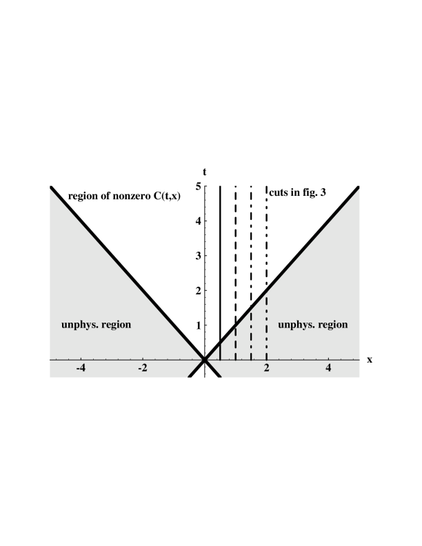
Clearly this is zero for space-like arguments, i.e., for . This free commutator function has support only in the unshaded area of Fig. 1, and it is singular at its boundaries (but zero outside).
We now turn to nontrivial spectral functions, which are more appropriate for a thermal system. The physical reason is, that at finite temperature particles are subject to collisions, hence their state of motion will change after a certain time. In a hot quantum system therefore the off-shell propagation of particles plays an important role. This off-shellness is contained in a continuous spectral function, which must not have an isolated -function like pole. In principle this means that at nonzero temperature every quantum system must be described on the same footing as a gas of resonances. However, this does not imply that thermal particles may decay – they are merely scattered thermally by the other components of the system.
Apart from this physically motivated use of continuous spectral functions at finite temperature, one may also adopt a mathematically rigorous stance. We do not elaborate on this, but rather quote the Narnhofer-Thirring theorem [5]. It states, that interacting systems at finite temperature cannot be described by particles with a sharp dispersion law, only non-interacting “hot” systems may have a -like spectral function. Ignoring this mathematical fact one finds as an echo serious infrared divergences in high temperature perturbative quantum chromo dynamics (QCD). Consequently, these unphysical singularities are naturally removed within an approach of finite temperature field theory with continuous mass spectrum [6, 7].
Thus, for a mathematical as well as a physical reason, finite temperature spectral functions are more complicated than those given in eq. (6). The question then arises, how much more complicated they have to be in order to be consistent with the requirements we have discussed above: Fully self consistent calculations of the corresponding spectral functions are very rare due to the numerical difficulties involved [7, 8, 9]. More often one uses an ansatz for such a function which involves only a small number of parameters which are then determined in a more or less “self”-consistent scheme.
As an example we consider two seemingly simplistic generalizations of the spectral functions in eq. (6), which involve only one additional parameter:
| (8) | |||||
| (9) | |||||
| (11) | |||||
where . These relativistic Breit-Wigner functions are somewhat oversimplified as compared with the real world: They attribute the same spectral width to very fast and very slow particles. Indeed, even when approximating a more sophisticated calculation of a spectral function by simple poles in the complex energy plane, one obtains a strongly momentum dependent spectral width parameter (see [7, pp. 350] for an example).
However, for some physical effects the influence of fast particles is reduced by Bose-Einstein or Fermi-Dirac distribution functions, such that one may use these simple spectral functions. Their constant spectral width parameters then may be considered as a parametrisation of the dominant low-energy phenomena. A good example for such a physical effect is the radiation of soft photons from a hot plasma, i.e., the “glow” of the plasma, where the ansatz of a constant spectral width parameter gives results comparable to the classical Landau-Pomeranchuk-Migdal effect [10].
It is a matter of a few lines to show, that the (anti-) commutator functions for the quantum fields defined by these spectral functions are
| (12) | |||||
| (13) |
These simple generalizations of the free spectral function therefore have the important property to preserve causality: Their Fourier transform vanishes for space-like arguments. Consequently, if these spectral functions are used to construct a generalized free field theory [6, 7], it will be local.
Let us note at this point, that the most general form of a spectral function which conforms with this requirement has been given in ref. [11]. We are not, however, interested in the most general spectral function, but in those which are only slightly more complicated than the free case.
III Hot gauge theory
To this end, we turn to study hot gauge theory, as discussed in the current literature [12, 13, 14, 15]. Naturally we cannot possibly check all the existing calculations of spectral functions, and therefore restrict ourselves to the most basic picture obtained in high-temperature QED. Up to a single difference this exactly comprises the fermion gauge boson spectral functions obtained in the hard thermal loop resummation scheme of QCD [13].
Let us first study the fermion of this model, which has a propagator [14]
| (14) | |||
| (15) |
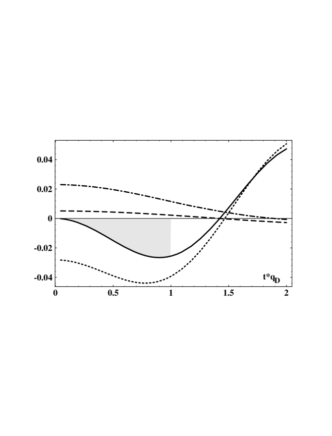
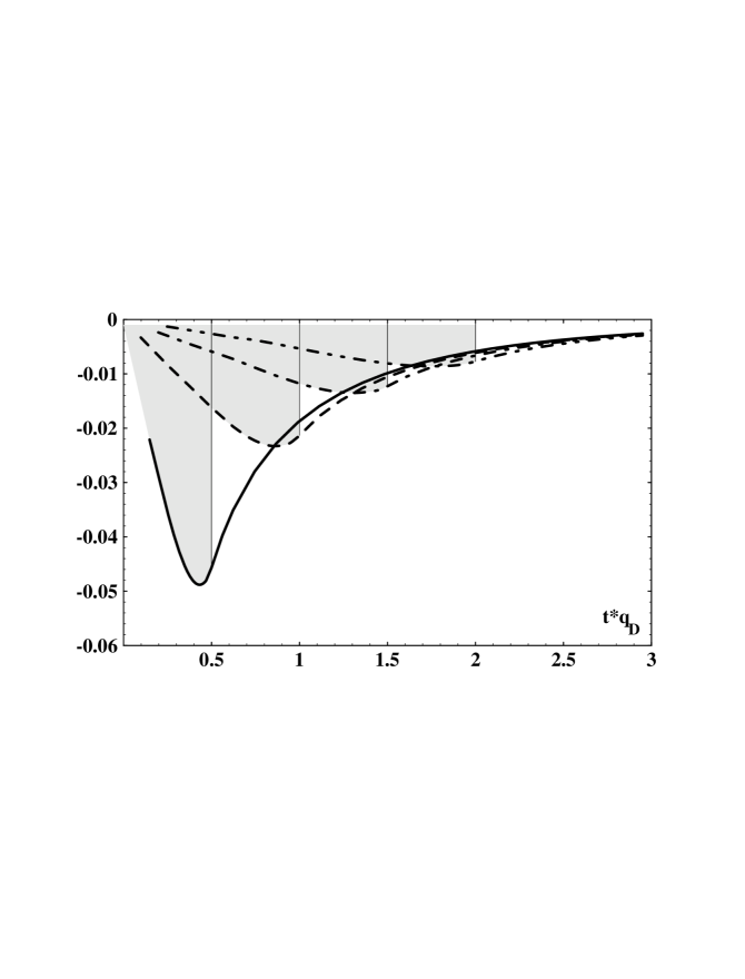
Here, , and is the Debye screening “mass”, proportional to the temperature. The spectral function of this propagator has a rather complicated structure, described in detail in ref. [14]: Four discrete poles at energies and with on the real axis; and a continuum for . Each of these pieces contributes to the Fourier transform as may be seen from the top panel of Fig. 2.
The four dimensional Fourier transform is a linear functional of the imaginary part of the propagator. Thus, each contribution to the spectral function may be transformed separately, and their sum then constitutes the total Fourier transform.
It is a priori clear that this total Fourier transform must be in agreement with the locality axiom. This follows from the fact, that is holomorphic in the forward tube, i.e., for timelike imaginary part of the four vector . However, only the sum of all contributions vanishes in the spacelike region, and therefore locality and causality are only guaranteed if spacelike and timelike four-momenta are taken into account in the propagator (15). A restriction in the fashion leads to a violation of causality.
It was already mentioned that there exists a difference between the hard thermal loop resummation (HTL) scheme and high temperature QED (or QCD). In the HTL method, the “dressed” propagators are used only for soft momenta which are smaller than , for high momenta one is required to use free propagators. The region of intermediate momenta is usually ignored in this method.
The locality axiom provides a convenient method to check for the validity of this approximation. To this end, we “patch” the free and resummed propagator together at the separation scale .
In the bottom panel of Fig.2 we show the anti-commutator function of two fermion fields using this prescription. Clearly, even the sum of all contributions does not vanish outside the physical region. We therefore conclude at this point, that no local quantum field theory can be constructed which conforms to the “patching” rule for the propagators. Consequently, one may not ignore the intermediate momentum region in hot gauge theory.
In the next step, we consider the gauge boson propagators, which for transverse and longitudinal degrees of freedom are
| (16) | |||||
| (17) |
is the bosonic Debye screening “mass”, which is proportional to the plasma frequency; it sets the only scale inherent to these propagators.
Both of them have a continuous imaginary part (= spectral function) in the regime , as well as a -function pole at some energy . The analytical structure of these propagators is quite complicated, but similar to the fermionic case it may be shown that they are holomorphic functions in the forward tube, and therefore their total Fourier transform is zero outside the physical region.
However, a restriction to spacelike momenta, i.e., to , leads to a violation of causality. A similar statement holds if these propagators are used only for timelike momenta, and consequently one should not consider plasmon propagation separately from “collective” effects.
The full gauge boson propagator is a linear combination of transverse and longitudinal piece with certain projection factors and a gauge parameter . In particular, the canonical 33-component is
| (18) |
We therefore have to study the Fourier transform of these products, and thereby concentrate on the transverse piece since its Fourier transform is numerically easier to obtain.
In the two panels of Fig. 2 we show the Fourier transform of the continuous part (spacelike momenta) and the plasmon part (timelike momenta) of the transverse piece of , i.e., of . The plot was made for several values of as function of (See Fig. 1 for the location of the displayed curves in the - plane). To each curve in the figure, we have added a thin vertical line separating the regions inside and outside the forward lightcone.
In the (shaded) region outside the forward cone, the two different contributions have the same sign and do not cancel each other in the total Fourier transform. It now remains the question, whether this is cured by taking into account the longitudinal piece of the propagator .
Obviously, since and are local by themselves, the violation of locality we saw above is due to the projection factors. Specifically it is due to the factor which introduces a branching-point singularity at in the forward tube. However, as is easily noted,
| (19) |
which implies that the branching point singularities cancel in the sum of transverse and longitudinal piece of eq. (18). We therefore term this violation of the locality axiom a purely kinematical one, which is cured by using transverse and longitudinal propagator on the same footing.
Consequently, the canonical gauge boson propagators of hot gauge theory are holomorphic functions for timelike imaginary part of , i.e., in their forward tube. Their Fourier transform vanishes for , and therefore they obey the locality axiom.
However, as pointed out before, this necessitates the use of the resummed propagator for all momenta. If for ”hard” momenta they are replaced by the free boson propagator, or forcibly set to zero, causality is violated. From a more mathematical viewpoint, the “patching” of propagators breaks the principle of analytical continuation. The violation of locality arises, because the “patched” propagators are no longer globally holomorphic in the forward tube.
Similarly, causality is violated if the propagators are restricted to spacelike or timelike momenta alone, as may be seen from Fig. 2 and 3. Another problem of remains even if the resummed propagators are used globally, i.e., for soft as well as for hard momenta: They do not conform with the relativistic Kubo-Martin-Schwinger boundary condition, which requires an exponential falloff in the high-momentum limit [16].
IV Conclusion
One may draw three conclusions from the present work. Firstly we find, that seemingly simplistic ansatz spectral functions as given in eqs. (11) obey the axiom of locality, i.e., they allow only causal non-locality. This makes them a reasonable starting point for any nonperturbative treatment of matter at high temperature.
The second conclusion is associated with the perturbative treatment of particles in hot gauge theory. Let us first discuss, whether a possible violation of locality in this case is of any relevance for measurable quantities: Following ref. [13] one may argue, that the gauge field itself has no physical meaning. However, the commutator of two magnetic field components in our example, where the commutator expectation value of different space-like components is zero, reads
| (20) |
This implies, that in the present example a non-vanishing commutator function of the gauge field outside the light cone generally leads to a non-vanishing commutator function for observable quantities. However, this statement has to be restricted: The purely kinematical violation of causality we observed when not combining transverse and longitudinal degrees of freedom will be canceled by moving to magnetic fields.
If we exclude this case, the violation we are discussing here would have the physical effect that the magnetic field could not be “measured” independently at two points with a space-like separation.
Another example is the electric field at space-time coordinate produced by a transverse -function perturbation at space-time coordinate . It is nothing but the time derivative of the Fourier transform of at point . Obviously a violation of the locality axiom implies, that this electric field may be measured already for times , and therefore it propagates faster than light (FTL).
According to our calculation such a violation may happen when plasmon propagation and collective effects are treated separately, i.e., when momenta are restricted to the timelike or spacelike region. Consequently such a separation should be done very carefully.
However, FTL propagation may also arise with propagators that are “patched” together: Resummed propagators for soft momenta, and free propagators for hard momenta. Our conclusion is, that to preserve causality one needs a spectral function which interpolates in a “smooth analytical way” between the high-momentum and the soft-momentum region, i.e., a naive “patching” may lead to unphysical results.
The third conclusion is associated with the separation into transverse and longitudinal degrees of freedom. From the standard literature one may get the impression, that they may be treated independently. In several applications of the propagators (17), one of the two is replaced by a free propagator. As we have argued, this is an invalid approximation: In order to preserve causality, longitudinal and transverse propagator must coincide in the limit .
Let us finally discuss a recipe to obtain local spectral functions. As noted before, the most general such function at finite temperature has been given in ref. [11, 16], where it was also shown that in principle an exponential falloff is necessary to obey the relativistic KMS-condition. For any non-local approximation (like e.g. obtained by “patching” propagators together) one may proceed as follows. In coordinate space, the non-local commutator function is multiplied by , then transformed back into momentum space. Equivalently, one may convolute the old momentum space propagator with the Fourier transform of such a -function.
We are currently exploring, how such a prescription would affect the “patched” spectral functions of hot gauge theory. Preliminary calculations show, that indeed this procedure leads to a spectral function which does not differ too much from eqn. (17), but which is nonzero for all values of the real energy parameter.
REFERENCES
-
[1]
Proceedings of the
Workshop on Perturbative Methods in Hot Gauge,
Winnipeg 1993;
Can.J.Phys. 71 Nos. 5 & 6 (1993) -
[2]
Proceedings of the
3rd Workshop on Thermal Field Theories
and their Applications, Banff 1993;
eds. F.C.Khanna, R.Kobes, G.Kunstatter und H.Umezawa
(World Scientific, Singapore 1994) -
[3]
Proceedings of the
4th Workshop on Thermal Field Theories
and their Applications, Dalian 1995 (to be published) -
[4]
J.Glimm and A.Jaffe, Quantum Physics
(Springer, New York 1981) -
[5]
H.Narnhofer, M.Requardt and W.Thirring,
Commun.Math.Phys. 92 (1983) 247 - [6] N.P.Landsman, Ann.Phys. 186 (1988) 141
- [7] P.A.Henning, Phys.Rep. 253 (1995) 235 – 380
- [8] P.A.Henning, Nucl.Phys. A546 (1992) 653
- [9] C.M.Korpa and R.Malfliet, Phys.Lett. B315 (1993) 209
-
[10]
P.A.Henning and E. Quack, Phys.Rev.Lett. 75 (1995) 2811,
extended version hep-ph 9508201 -
[11]
J.Bros and D.Buchholz, Z.Physik C 55 (1992) 509;
see also hep-th 9511202 and Ann.Inst. H.Poincaré 64 (1996) in press. - [12] H.A.Weldon, Phys.Rev. D 26 (1982) 1394
- [13] R.Pisarski, Physica A 158 (1989) 146
- [14] H.A.Weldon, Phys.Rev. D 47 (1989) 2410
- [15] J.P.Blaizot and E.Iancu, CEA Saclay Preprint T95/087
- [16] J.Bros and D.Buchholz, Nucl.Phys. B429 (1994) 291
Acknowledgements
We thank D.Buchholz for alerting us to the possible violation of locality when using approximate spectral functions. One of us (P.A.H.) wishes to express his gratitude to the members of the Service Physique Theorique in Saclay for their kind hospitality.
Gratefully acknowledged are stimulating discussions of this work with H.A.Weldon, R.Pisarski, L.McLerran and J.P.Blaizot on occasion of the VIIth Max-Born Symposium in Karpacz/Poland. Finally, thanks to J.Lindner for his comments on the manuscript.

Top panel: resummed propagator (15) used for all momenta;
bottom panel: (15) for momenta ,
otherwise free propagator.
Vertical lines at discontinuity omitted in the top panel.
Dotted line: “particle” contribution, dashed line “hole”
contribution, dash-dotted line continuum contribution (see text and ref.
[14]).
Continuous line: Sum of the three pieces, unphysical contribution shaded.
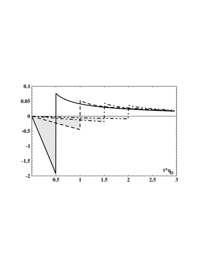
Top panel: continuous part (spacelike momenta);
bottom panel: plasmon part (timelike momenta),
-functions at removed. Note the two
different vertical scales in the bottom panel.
Plotted for = 0.5 (continuous), 1.0 (dashed), 1.5 (dash-dotted)
and 2.0 (dash-double-dotted).
Contributions outside the forward lightcone are shaded.