Transverse spin and transverse momenta
in hard scattering processes

Abstract

Inclusive and semi-inclusive deep inelastic leptoproduction offers possibilities to study details of the quark and gluon structure of the hadrons involved. In many of these experiments polarization is an essential ingredient. We also emphasize the dependence on transverse momenta of the quarks, which leads to azimuthal asymmetries in the produced hadrons.

October 1995
NIKHEF 95-057
hep-ph/9510317

Talk presented at the workshop on Prospects of Spin Physics at HERA, 28-31 August 1995, DESY (Hamburg), Germany

Transverse spin and transverse momenta

in hard scattering processes

P.J. Mulders
National Institute for Nuclear Physics and High-Energy Physics
(NIKHEF), P.O. Box 41882, NL-1009 DB Amsterdam, the Netherlands
and
Department of Physics and Astronomy, Free University
De Boelelaan 1081, NL-1081 HV Amsterdam, the Netherlands

1 Introduction

Hard processes using electroweak probes are very well suited to probe the quark and gluon structure of hadrons. The leptonic part is known, determining the kinematics of the electroweak probe. Examples of such processes are

• Lepton-hadron scattering (DIS)

  $$\gamma^{\ast}(q)+H\ \longrightarrow\ h+X\qquad\qquad(-q^{2}\equiv Q^{2}\geq 0)$$

• Drell-Yan scattering (DY)

  $$H_{A}+H_{B}\ \longrightarrow\ \gamma^{\ast}(q)+X\qquad\qquad(q^{2}\equiv Q^{2}\geq 0)$$

• Electron-positron annihilation

  $$\gamma^{\ast}(q)\ \longrightarrow\ h_{1}+h_{2}+X\qquad\qquad(q^{2}\equiv Q^{2}\geq 0)$$

The interaction of the electroweak probe with quarks is known.

We consider deep inelastic processes where $Q$ is considerably larger (how much is mostly an empirical fact) than the typical hadronic scale $\Lambda$, which is of order 1 GeV. The large momentum $Q$ makes it feasible to do the calculation within the framework of QCD. One writes down a diagrammatic expansion of the hard scattering amplitude (actually the squared amplitude), dividing it into hard and soft parts. The simplest (parton model diagram) for semi-inclusive $\ell H$ scattering is shown in Fig. 1.

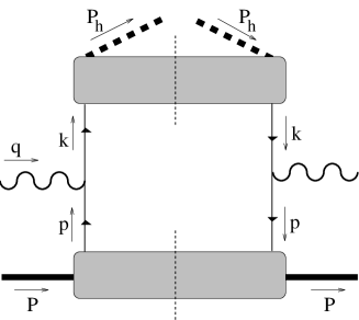
Figure 1: The parton level diagram for semi-inclusive deep inelastic scattering

The photon couples into the hard part, containing quark and gluon lines, while hadrons couple into soft parts, represented by a blob connecting hadron lines and quark and gluon lines for which the momenta satisfy $p_{i}\cdot p_{j}\sim\Lambda^{2}\ll Q^{2}$. For the calculation of the hard part one can use the QCD Feynman rules, while for the soft parts simply the definition enters, being expectation values of quark and gluon fields in hadron states.

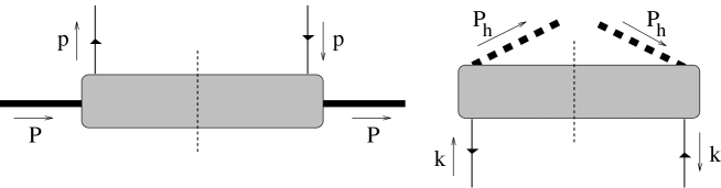
Figure 2: Quark-quark correlation function giving quark distributions (left) and fragmentation functions (right)

It turns out that at tree level the leading diagrams contain soft parts that are quark-quark correlation functions of the type shown in Fig. 2, given by [1, 2, 3]

$$\Phi_{ij}(p,P,S)=\frac{1}{(2\pi)^{4}}\int d^{4}x\ e^{i\,p\cdot x}\langle P,S|\overline{\psi}_{j}(0)\,\psi_{i}(x)|P,S\rangle,$$ (1)

where a summation over color indices is implicit, and

$$\Delta_{ij}(k,P_{h},S_{h})=\sum_{X}\frac{1}{(2\pi)^{4}}\int d^{4}x\ e^{ik\cdot x}\,\langle 0|\psi_{i}(x)|P_{h},S_{h};X\rangle\langle P_{h},S_{h};X|\overline{\psi}_{j}(0)|0\rangle$$ (2)

where an averaging over color indices is implicit. In both definitions flavor indices are suppressed and also the path ordered link operator needed to make the bilocal matrix element color gauge-invariant is omitted.

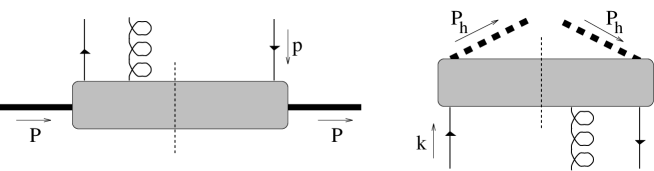
Figure 3: Quark-quark-gluon correlation functions contributing in hard scattering processes at subleading order.

The large scale $Q$ leads to an ordering of the terms in the diagrammatic expansion [4] in powers of $1/Q$, $\alpha_{s}$ and $\alpha_{s}\ln Q^{2}$. Writing down the simplest diagram where a photon is absorbed on a quark one ends up with the combination of soft parts in Fig. 2. Gluonic corrections in the hard QCD part of the process can be absorbed in a scale dependence of the soft parts, at least at leading order (factorization). At order $1/Q$ also quark-quark-gluon correlation functions (shown in Fig. 3) appear. These can be rewritten in quark-quark correlation functions using the QCD equations of motion, provided that one does include the dependence on the transverse momenta of the quarks.

Next step is the analysis of the correlation functions including the transverse momentum dependence [5, 6]. It is convenient to parametrize the momenta in terms of lightcone coordinates, $p=[p^{-},p^{+},\mbox{\boldmath$p$}_{T}]$ with $p^{\pm}=(p^{0}\pm p^{3})/\sqrt{2}$. Choosing a frame in which the hadrons are collinear one writes for the hadrons and virtual photon in $\ell H$ scattering,

$$P \ =\ \left[\frac{x_{\scriptscriptstyle B}M^{2}}{A\sqrt{2}},\frac{A}{x_{\scriptscriptstyle B}\sqrt{2}},\mbox{$\bf 0$}_{T}\right]\ \equiv\ \frac{Q}{x_{\scriptscriptstyle B}\sqrt{2}}\,n_{+}+\frac{x_{\scriptscriptstyle B}M^{2}}{Q\sqrt{2}}\,n_{-},$$ (3)

$$P_{h} \ =\ \left[\frac{z_{h}Q^{2}}{A\sqrt{2}},\frac{AM_{h}^{2}}{z_{h}Q^{2}\sqrt{2}},\mbox{$\bf 0$}_{T}\right]\ \equiv\ \frac{z_{h}\,Q}{\sqrt{2}}\,n_{-}+\frac{M_{h}^{2}}{z_{h}\,Q\sqrt{2}}\,n_{+},$$ (4)

$$q \ =\ \left[\frac{Q^{2}}{A\sqrt{2}},-\frac{A}{\sqrt{2}},\mbox{\boldmath$q$}_{T}\right]\ =\ \frac{Q}{\sqrt{2}}\,n_{+}-\frac{Q}{\sqrt{2}}\,n_{-}+q_{\scriptstyle T}.$$ (5)

Note that in a frame in which $P$ and $q$ have no transverse momenta, the outgoing hadron has a transverse momentum $\mbox{\boldmath$P$}_{h\perp}=-z\mbox{\boldmath$q$}_{T}$. The calculation of the diagrams involves an integral over soft parts,

$$\Phi^{[\Gamma]}(x,\mbox{\boldmath$p$}_{T}) = \left.\frac{1}{2}\int dp^{-}\ Tr(\Phi\,\Gamma)\right|_{p^{+}=xP^{+},\ \mbox{\boldmath$p$}_{T}},$$ (6)

$$\Delta^{[\Gamma]}(z,\mbox{\boldmath$k$}_{T}) = \left.\frac{1}{4z}\int dk^{+}\ Tr(\Delta\,\Gamma)\right|_{k^{-}=P_{h}^{-}/z,\ \mbox{\boldmath$k$}_{T}}.$$ (7)

Depending on the Dirac matrix $\Gamma$, these correlation functions are parametrized in terms of distribution and fragmentation functions, e.g. for a polarized spin 1/2 target with spin vector $S=\left[-\lambda\,M/2P^{+},\lambda\,P^{+}/M,\mbox{\boldmath$S$}_{T}\right]$ with $\lambda^{2}+\mbox{\boldmath$S$}_{T}^{2}$ = 1,

$$\Phi^{[\gamma^{+}]}(x,\mbox{\boldmath$p$}_{T})=f_{1}(x,\mbox{\boldmath$p$}_{T}),$$ (8)

$$\Phi^{[\gamma^{+}\gamma_{5}]}(x,\mbox{\boldmath$p$}_{T})=\lambda\,g_{1L}(x,\mbox{\boldmath$p$}_{T})+g_{1T}(x,\mbox{\boldmath$p$}_{T})\,\frac{(\mbox{\boldmath$p$}_{T}\cdot\mbox{\boldmath$S$}_{T})}{M}\equiv g_{1s}(x,\mbox{\boldmath$p$}_{T}),$$ (9)

$$\Phi^{[i\sigma^{i+}\gamma_{5}]}(x,\mbox{\boldmath$p$}_{T})=S_{\scriptstyle T}^{i}\,h_{1T}(x,\mbox{\boldmath$p$}_{T})+\frac{p_{\scriptstyle T}^{i}}{M}\,h_{1s}^{\perp}(x,\mbox{\boldmath$p$}_{T}),$$ (10)

$$\Phi^{[1]}(x,\mbox{\boldmath$p$}_{T})=\frac{M}{P^{+}}\,e(x,\mbox{\boldmath$p$}_{T})$$ (11)

$$\Phi^{[\gamma^{i}]}(x,\mbox{\boldmath$p$}_{T})=\frac{p_{\scriptstyle T}^{i}}{P^{+}}\,f^{\perp}(x,\mbox{\boldmath$p$}_{T}),$$ (12)

$$\Phi^{[\gamma^{i}\gamma_{5}]}(x,\mbox{\boldmath$p$}_{T})=\frac{M\,S_{\scriptstyle T}^{i}}{P^{+}}\,g_{\scriptstyle T}^{\prime}(x,\mbox{\boldmath$p$}_{T})+\frac{p_{\scriptstyle T}^{i}}{P^{+}}\,g_{s}^{\perp}(x,\mbox{\boldmath$p$}_{T})$$ (13)

$$\Phi^{[i\sigma^{ij}\gamma_{5}]}(x,\mbox{\boldmath$p$}_{T})=\frac{S_{\scriptstyle T}^{i}p_{\scriptstyle T}^{j}-p_{\scriptstyle T}^{i}S_{\scriptstyle T}^{j}}{P^{+}}\,h_{\scriptstyle T}^{\perp}(x,\mbox{\boldmath$p$}_{T})$$ (14)

$$\Phi^{[i\sigma^{+-}\gamma_{5}]}(x,\mbox{\boldmath$p$}_{T})=\frac{M}{P^{+}}\,h_{s}(x,\mbox{\boldmath$p$}_{T}).$$ (15)

In naming the functions we have extended the scheme proposed by Jaffe and Ji [7] for the $\mbox{\boldmath$k$}_{T}$-integrated functions. Depending on the Lorentz structure of the Dirac matrices $\Gamma$ the parametrization involves powers $(1/P^{+})^{t-2}$, where $t$ is referred to as ’twist’. Integrated over $k_{T}$ and taking moments in $x$ it corresponds to the OPE ’twist’ of the (in that case) local operators. When everything is done it will turn out that the factors $1/P^{+}$ give rise to factors $1/Q$ in the cross sections. The leading projections $\Phi^{[\gamma^{+}]}$, $\Phi^{[\gamma^{+}\gamma_{5}]}$ and $\Phi^{[i\sigma^{+i}\gamma_{5}]}$ can be interpreted as quark momentum densities, namely the unpolarized distribution, the chirality (for massless quarks helicity) distribution and the transverse spin distribution, respectively.

For the fragmentation functions one has an analogous analysis, which for unpolarized final state hadrons yields

$$\Delta^{[\gamma^{-}]}(z,\mbox{\boldmath$k$}_{T})=D_{1}(z,-z\mbox{\boldmath$k$}_{T}),$$ (16)

$$\Delta^{[i\sigma^{i-}\gamma_{5}]}(z,\mbox{\boldmath$k$}_{T})=\frac{\epsilon_{\scriptscriptstyle T}^{ij}k_{Tj}}{M_{h}}\,H_{1}^{\perp}(z,-z\mbox{\boldmath$k$}_{T}),$$ (17)

$$\Delta^{[1]}(z,\mbox{\boldmath$k$}_{T})=\frac{M_{h}}{P_{h}^{-}}\,E(z,-z\mbox{\boldmath$k$}_{T}),$$ (18)

$$\Delta^{[\gamma^{i}]}(z,\mbox{\boldmath$k$}_{T})=\frac{k_{T}^{i}}{P_{h}^{-}}\,D^{\perp}(z,-z\mbox{\boldmath$k$}_{T}),$$ (19)

$$\Delta^{[i\sigma^{ij}\gamma_{5}]}(z,\mbox{\boldmath$k$}_{T})=\frac{M_{h}\,\epsilon_{\scriptscriptstyle T}^{ij}}{P_{h}^{-}}\,H(z,-z\mbox{\boldmath$k$}_{T}).$$ (20)

Here each power $1/P_{h}^{-}$ leads to a factor $1/Q$ in the cross section. The functions $H_{1}^{\perp}$ and $H$ have no equivalent for distribution functions. They are allowed for the fragmentation functions because time reversal invariance cannot be used in the analysis for $\Delta$ which involves out-states $|P_{h},X\rangle$.

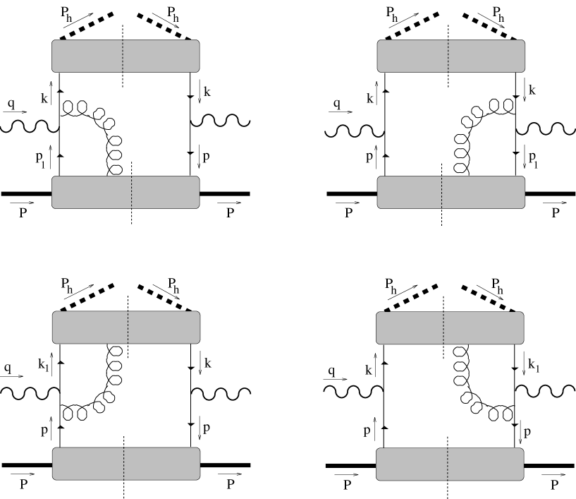
Figure 4: Diagrams contributing at order $1/Q$ in semi-inclusive deep inelastic scattering

Putting everything together [8], the result of the tree-level calculation up to order $1/Q$ is given by the diagram in Fig. 1 and the diagrams shown in Fig. 4 (plus of course antiquark diagrams). The result involves combinations of the distribution and fragmentation functions defined above. The inclusion of qqG-correlation functions of the type in Fig. 3 and their relation to qq-correlations through the equations of motion are essential to ensure electromagnetic gauge invariance. We give 3 specific examples of cross sections. The first is well-known, being the result for inclusive $\ell H$ scattering up to order $1/Q$ including polarization. Using the scaling variables $x=Q^{2}/2P\cdot q$ and $y=P\cdot k/P\cdot q$ one obtains

$$\frac{d\sigma}{dx_{\scriptscriptstyle B}\,dy} = \frac{4\pi\alpha^{2}\,s}{Q^{4}}\ \Biggl{\{}\,\left\lgroup\frac{y^{2}}{2}+1-y\right\rgroup x_{\scriptscriptstyle B}f_{1}(x_{\scriptscriptstyle B})+\lambda_{e}\,\lambda\,y\left\lgroup 1-\frac{y}{2}\right\rgroup x_{\scriptscriptstyle B}g_{1}(x_{\scriptscriptstyle B})$$ (21)

$$-\lambda_{e}\,|\mbox{\boldmath$S$}_{\perp}|\,\frac{M}{Q}\,2\,y\sqrt{1-y}\,\cos(\phi_{s})\,x_{\scriptscriptstyle B}^{2}\,g_{T}(x_{\scriptscriptstyle B})\,\Biggr{\}}.$$

As indicated before, the twist-3 function in $\Phi^{[\gamma^{i}\gamma_{5}]}$ surviving after $k_{T}$-integration, $g_{T}=g_{T}^{\prime}+(\mbox{\boldmath$k$}_{T}^{2}/2M^{2})\,g_{T}^{\perp}$, appears at subleading order. Reinstating the summation over quark flavors and identifying the result with the most general cross sections, expressed in terms of structure functions, one obtains

$$\frac{F_{2}(x_{\scriptscriptstyle B},Q^{2})}{x_{\scriptscriptstyle B}}=2\,F_{1}(x_{\scriptscriptstyle B},Q^{2})=\sum_{a}e_{a}^{2}\,\left(f_{1}^{(a)}(x_{\scriptscriptstyle B})+\bar{f}_{1}^{(a)}(x_{\scriptscriptstyle B})\right),$$ (22)

$$2\,\mbox{\large{\em g}}_{1}(x_{\scriptscriptstyle B},Q^{2})=\sum_{a}e_{a}^{2}\,\left(g_{1}^{(a)}(x_{\scriptscriptstyle B})+\bar{g}_{1}^{(a)}(x_{\scriptscriptstyle B})\right),$$ (23)

$$\mbox{\large{\em g}}_{T}(x_{\scriptscriptstyle B},Q^{2})=\mbox{\large{\em g}}_{1}(x_{\scriptscriptstyle B},Q^{2})+\mbox{\large{\em g}}_{2}(x_{\scriptscriptstyle B},Q^{2})=\frac{1}{2}\sum_{a}e_{a}^{2}\,\left(g_{T}^{(a)}(x_{\scriptscriptstyle B})+\bar{g}_{T}^{(a)}(x_{\scriptscriptstyle B})\right).$$ (24)

The second example is semi-inclusive scattering including the dependence on the transverse momentum $\mbox{\boldmath$P$}_{h\perp}$ of the detected hadron [9, 10]. For this we assume a gaussian transverse momentum dependence for the quark distribution and fragmentation functions,

$$f(x,\mbox{\boldmath$p$}_{T}^{2}) = f(x)\,\frac{R_{H}^{2}}{\pi}\,\exp(-R_{H}^{2}\mbox{\boldmath$p$}_{T}^{2})\equiv f(x)\,{\cal G}(|\mbox{\boldmath$p$}_{T}|;R_{H}),$$ (25)

$$D(z,z^{2}\mbox{\boldmath$k$}_{T}^{2}) = D(z)\,\frac{R_{h}^{2}}{\pi\,z^{2}}\,\exp(-R_{h}^{2}\mbox{\boldmath$k$}_{T}^{2})=\frac{D(z)}{z^{2}}\,{\cal G}(|\mbox{\boldmath$k$}_{T}|;R_{h})=D(z)\,{\cal G}\left(z|\mbox{\boldmath$k$}_{T}|;\frac{R_{h}}{z}\right).$$ (26)

This enables us to express the results in the $\mbox{\boldmath$p$}_{T}$-integrated distributions and a (normalized) gaussian distribution, while we can evaluate the complex-looking convolutions in transverse momenta that appear in the cross sections replacing them by a simple gaussian distribution in $Q_{T}$. The result for the cross section is

$$\frac{d\sigma}{dx_{\scriptscriptstyle B}\,dy\,dz_{h}\,d^{2}\mbox{\boldmath$P$}_{h\perp}}\ =\ \frac{4\pi\alpha^{2}\,s}{Q^{4}}\,\sum_{a,\bar{a}}e_{a}^{2}\,\left\lgroup\frac{y^{2}}{2}+1-y\right\rgroup\,x_{\scriptscriptstyle B}f_{1}^{a}(x_{\scriptscriptstyle B})\,D^{a}_{1}(z_{h})\,\frac{{\cal G}(Q_{T};R)}{z_{h}^{2}}$$

$$\qquad\quad\mbox{}-\frac{4\pi\alpha^{2}\,s}{Q^{4}}\,\lambda\,\sum_{a,\bar{a}}e_{a}^{2}\,(1-y)\,\sin(2\phi_{h})\,\frac{Q_{T}^{2}\,R^{4}}{MM_{h}\,R_{H}^{2}\,R_{h}^{2}}\,x_{\scriptscriptstyle B}h_{1L}^{\perp\,a}(x_{\scriptscriptstyle B})H_{1}^{\perp\,a}(z_{h})\,\frac{{\cal G}(Q_{T};R)}{z_{h}^{2}}$$

$$\qquad\quad\mbox{}-\frac{4\pi\alpha^{2}\,s}{Q^{4}}\,|\mbox{\boldmath$S$}_{\perp}|\,\sum_{a,\bar{a}}e_{a}^{2}\,\Biggl{\{}(1-y)\,\sin(\phi_{h}+\phi_{s})\,\frac{Q_{T}\,R^{2}}{M_{h}\,R_{h}^{2}}\,x_{\scriptscriptstyle B}h^{a}_{1}(x_{\scriptscriptstyle B})H_{1}^{\perp\,a}(z_{h})$$

$$\qquad\qquad\qquad\quad+(1-y)\,\sin(3\phi_{h}-\phi_{s})\,\frac{Q_{T}^{3}\,R^{6}}{2M^{2}M_{h}\,R_{H}^{4}\,R_{h}^{2}}\,x_{\scriptscriptstyle B}h_{1T}^{\perp\,a}(x_{\scriptscriptstyle B})H_{1}^{\perp\,a}(z_{h})\Biggr{\}}\,\frac{{\cal G}(Q_{T};R)}{z_{h}^{2}}$$

$$\qquad\quad\mbox{}+\frac{4\pi\alpha^{2}\,s}{Q^{4}}\,\lambda_{e}\lambda\,\sum_{a,\bar{a}}e_{a}^{2}\,y\left(1-\frac{y}{2}\right)\,x_{\scriptscriptstyle B}\,g^{a}_{1L}(x_{\scriptscriptstyle B})\,D^{a}_{1}(z_{h})\,\frac{{\cal G}(Q_{T};R)}{z_{h}^{2}}$$

$$\qquad\quad\mbox{}+\frac{4\pi\alpha^{2}\,s}{Q^{4}}\,|\mbox{\boldmath$S$}_{\perp}|\,\sum_{a,\bar{a}}e_{a}^{2}\,y\left(1-\frac{y}{2}\right)\,\cos(\phi_{h}-\phi_{s})\,\frac{Q_{T}\,R^{2}}{M\,R_{H}^{2}}\,g^{a}_{1T}(x_{\scriptscriptstyle B})D^{a}_{1}(z_{h})\,\frac{{\cal G}(Q_{T};R)}{z_{h}^{2}}.$$ (27)

We see that all six twist-two $x$- and $\mbox{\boldmath$p$}_{T}$-dependent quark distribution functions for a spin 1/2 hadron can be accessed in leading order asymmetries if one considers lepton and hadron polarizations. One of the asymmetries involves the transverse spin distribution $h_{1}^{a}$ [11]. On the production side, only two different fragmentation functions are involved, the familiar unpolarized fragmentation function $D_{1}^{a}$ and the fragmentation function $H_{1}^{\perp a}$. The latter is one of the functions which depends on interactions and is allowed in the fragmentation process because one cannot use time-reversal invariance.

As our last example, we give the extension of the above result up to order $1/Q$ for an unpolarized nucleon target. One obtains

$$\frac{d\sigma}{dx_{\scriptscriptstyle B}\,dy\,dz_{h}\,d^{2}\mbox{\boldmath$P$}_{h\perp}}\ =\ \frac{4\pi\alpha^{2}\,s}{Q^{4}}\,\sum_{a,\bar{a}}e_{a}^{2}\,\Biggl{\{}\left\lgroup\frac{y^{2}}{2}+1-y\right\rgroup\,x_{\scriptscriptstyle B}f_{1}^{a}(x_{\scriptscriptstyle B})\,D^{a}_{1}(z_{h})$$

$$\qquad\mbox{}-2(2-y)\sqrt{1-y}\,\cos(\phi_{h})\,\frac{Q_{T}}{Q}\Biggl{(}\,\frac{R^{2}}{R_{H}^{2}}\,x_{\scriptscriptstyle B}^{2}f^{\perp\,a}(x_{\scriptscriptstyle B})D^{a}_{1}(z_{h})-\frac{R^{2}}{R_{h}^{2}}\,x_{\scriptscriptstyle B}f^{a}_{1}(x_{\scriptscriptstyle B})\,\frac{\tilde{D}^{\perp\,a}(z_{h})}{z_{h}}\Biggr{)}$$

$$\qquad\mbox{}-\lambda_{e}\,2y\sqrt{1-y}\,\sin\phi_{h}\,\frac{Q_{T}}{Q}\,\frac{M\,R^{2}}{M_{h}\,R_{h}^{2}}\,x_{\scriptscriptstyle B}^{2}\,\tilde{e}^{a}(x_{\scriptscriptstyle B})\,H_{1}^{\perp\,a}(z_{h})\Biggr{\}}\,\frac{{\cal G}(Q_{T};R)}{z_{h}^{2}},$$ (28)

The $\langle\cos(\phi_{h})\rangle$ asymmetry in unpolarized leptoproduction, unfortunately is rather complicated, involving one twist-three distribution function ($f^{\perp a}$) and one twist-three fragmentation function ($D^{\perp a}$) [12]. It is important to point out, however, that the $\langle\cos(\phi_{h})\rangle$ asymmetry is not only a kinematical effect [13]. It reduces to a kinematical factor only depending on $y$ and $Q^{2}$ when the interaction-dependent pieces in the twist-three functions [8] are set to zero, $\tilde{f}^{\perp a}$ = $f^{\perp a}-f_{1}^{a}/x_{\scriptscriptstyle B}$ = 0 and $\tilde{D}^{\perp a}$ = $D^{\perp a}-z_{h}\,D_{1}^{\perp a}$ = 0. At order $1/Q$ there is no $\langle\cos(2\phi_{h})\rangle$ asymmetry in the deep-inelastic leptoproduction cross section. For polarized leptons and unpolarized targets a $\langle\sin(\phi_{h})\rangle$ asymmetry is found [14], involving the interaction dependent part of the distribution function $e^{a}$, $\tilde{e}^{a}$ = $e^{a}-(m/M)f_{1}^{a}$, and the time-reversal odd fragmentation function $H_{1}^{\perp a}$. Noteworthy is that it is the same fragmentation function that appears in several of the leading azimuthal asymmetries for polarized targets.

This work is part of the research program of the foundation for Fundamental Research of Matter (FOM) and the National Organization for Scientific Research (NWO).

References

[1]
D.E. Soper, Phys. Rev. D 15 (1977) 1141; Phys. Rev. Lett. 43
(1979) 1847