Excited states of heavy baryons in the Skyrme model

Abstract

We obtain the spectra of excited heavy baryons containing one heavy quark by quantizing the exactly-solved heavy meson bound states to Skyrme soliton. The results are comparable to the recent experimental observations and quark model predictions, and are consistent with the heavy quark spin symmetry. However, somewhat large dependence of the results on the heavy quark mass strongly calls for the incorporation of the soliton-recoil effects.

I Introduction

Up to the present, most ground state charm baryons containing one $c$-quark, from $\Lambda_{c}^{+}$ to $\Omega_{c}^{0}$, have been observed [1]. There have been much efforts to find excited charm baryons and recently the experimental evidences for $\Sigma_{c}^{*}(2530)$ [2], $\Lambda^{*}_{c}(2593)$ and $\Lambda^{*}_{c}(2625)$ [3, 4, 5, 6] are reported. Although their quantum numbers are not identified yet, the spin-parity of the $\Sigma^{*}_{c}(2530)$ is interpreted as $j^{\pi}=\frac{3}{2}{}^{+}$, and $\Lambda^{*}_{c}(2593)$ and $\Lambda^{*}_{c}(2625)$ decaying to $\Lambda_{c}^{+}\pi^{+}\pi^{-}$ are regarded as candidates for $j^{\pi}=\frac{1}{2}{}^{-}$ and $\frac{3}{2}{}^{-}$ excited states, respectively, in accordance with the quark model predictions [7, 8, 9, 10, 11, 12]. The small mass splittings between $\Sigma^{*}_{c}(2530)$ and $\Sigma_{c}(2453)$ and between $\Lambda_{c}^{*}(2593)$ and $\Lambda_{c}^{*}(2625)$ are consistent with the heavy quark spin symmetry [13, 14], according to which the hadrons come in degenerate doublets with total spin $j_{\pm}=j_{\ell}\pm\frac{1}{2}$ (unless $j_{\ell}$, the total angular momentum of the light degrees of freedom, is zero) in the limit of the heavy quark mass going to infinity.

On the other hand, the excited heavy baryons have been extensively studied not only in various quark/bag models [7, 8, 9, 10, 11, 12, 15] but also in heavy hadron chiral perturbation theory [16] and in the bound state approach of the Skyrme model [17, 18, 19, 20]. In the bound state model, the heavy baryons are described by bound states of heavy mesons and a soliton [21, 22]. A natural explanation of low-lying $\Lambda(1405)$ is one of the success of the bound state approach [23], where this $j^{\pi}=\frac{1}{2}{}^{-}$ state is described by a loosely bound $S$-wave $K$ meson to soliton. The same picture was straightforwardly applied to the excited $\Lambda_{c}^{*}(\frac{1}{2}{}^{-})$ in Ref. [17]. The lack of the heavy quark symmetry in this first trial is later supplied by treating the heavy vector mesons on the same footing as the heavy pseudoscalar mesons [22], and a generic structure of the heavy baryon spectrum of orbitally excited states is established [18].

However, these works were done under the approximation that both the soliton and the heavy mesons are infinitely heavy and so they sit on top of each other. It is evident that this approximation cannot describe well the orbitally and/or radially excited states due to the ignorance of any kinetic effects. In Ref. [19], the kinetic effects for the excited states are estimated by approximating the static potentials for the heavy mesons to the quadratic form with the curvature determined at the origin. Such a harmonic oscillator approximation is valid only when the heavy mesons are sufficiently massive so that their motions are restricted to a very small range. The situation is improved in Ref. [20] by making an approximate Schrödinger-like equation and by incorporating the light vector mesons. In a recent paper [24], we have obtained all the energy levels of the heavy meson bound states by solving exactly the equations of motion from a given model Lagrangian without using any approximations. (See also Refs. [25, 26].) In this paper, we quantize those states by following the standard collective coordinate quantization method to investigate the excited heavy baryon spectra.

In the next section, we briefly describe our model Lagrangian and the way of solving the equations of motion to obtain the bound states. Then, in Sec. III, we quantize the soliton–heavy-meson bound system based on the standard collective coordinate quantization method and derive the mass formula. The resulting mass spectra of $\Lambda_{c}$, $\Sigma_{c}$, $\Lambda_{b}$, and $\Sigma_{b}$ baryons are presented in Sec. IV and compared with the recent experimental observations and with the quark model predictions. Some detailed expressions are given in Appendix.

II The model

We will work with a simple effective chiral Lagrangian of Goldstone mesons and heavy mesons [27]:

$$\begin{array}[]{rcl}{\cal L}&=&{\cal L}^{\text{SM}}_{M}+D_{\mu}\Phi D^{\mu}\Phi^{\dagger}-m_{\Phi}^{2}\Phi\Phi^{\dagger}-{\textstyle\frac{1}{2}}\Phi^{*\mu\nu}\Phi^{*\dagger}_{\mu\nu}+m_{\Phi^{*}}^{2}\Phi^{*\mu}\Phi^{*\dagger}_{\mu}\\ &&\mbox{}+f_{Q}(\Phi A^{\mu}\Phi^{*\dagger}_{\mu}+\Phi^{*}_{\mu}A^{\mu}\Phi^{\dagger})+{\textstyle\frac{1}{2}}g_{Q}\varepsilon^{\mu\nu\lambda\rho}(\Phi^{*}_{\mu\nu}A_{\lambda}\Phi^{*\dagger}_{\rho}+\Phi^{*}_{\rho}A_{\lambda}\Phi^{*\dagger}_{\mu\nu}).\end{array}$$ (1)

Here, ${\cal L}^{\text{SM}}_{M}$ is an effective chiral Lagrangian of Goldstone pions presented by an $SU(2)$ matrix field $U=\exp(i\mathchoice{{\hbox{\boldmath$\displaystyle\tau$}}}{{\hbox{\boldmath$\textstyle\tau$}}}{{\hbox{\boldmath$\scriptstyle\tau$}}}{{\hbox{\boldmath$\scriptscriptstyle\tau$}}}\cdot\mathchoice{{\hbox{\boldmath$\displaystyle\pi$}}}{{\hbox{\boldmath$\textstyle\pi$}}}{{\hbox{\boldmath$\scriptstyle\pi$}}}{{\hbox{\boldmath$\scriptscriptstyle\pi$}}}/f_{\pi})$, which is simply taken as the Skyrme model Lagrangian,

$${\cal L}^{\text{SM}}_{M}=\frac{f_{\pi}^{2}}{4}\,\text{Tr}\,(\partial_{\mu}U^{\dagger}\partial^{\mu}U)+\frac{1}{32e^{2}}\,\text{Tr}\,[U^{\dagger}\partial_{\mu}U,U^{\dagger}\partial_{\nu}U]^{2},$$ (2)

with the pion decay constant $f_{\pi}$ and the Skyrme parameter $e$. With the help of the Skyrme term, it supports a stable baryon-number-1 soliton solution under the hedgehog configuration

$$U_{0}({\bf r})=\exp[i\mathchoice{{\hbox{\boldmath$\displaystyle\tau$}}}{{\hbox{\boldmath$\textstyle\tau$}}}{{\hbox{\boldmath$\scriptstyle\tau$}}}{{\hbox{\boldmath$\scriptscriptstyle\tau$}}}\cdot\hat{\bf r}F(r)],$$ (3)

where $F(r)$ satisfies the boundary conditions, $F(0)=\pi$ and $F(\infty)=0$.

The heavy pseudoscalar and vector mesons containing a heavy quark $Q$ are represented by anti-isodoublet fields $\Phi$ and $\Phi^{*}_{\mu}$, with their masses $m_{\Phi}$ and $m_{\Phi^{*}}$, respectively. As an example, in case of $Q=c$, they are $D$ and $D^{*}$ meson anti-doublets,

$$\Phi=(D^{0},D^{+})\quad\text{ and }\quad\Phi^{*}=(D^{*0},D^{*+}).$$ (4)

The chiral transformations of the fields are defined as

$$\begin{array}[]{l}\xi\rightarrow L\xi h^{\dagger}=h\xi R^{\dagger},\\ \Phi,\>\Phi^{*}_{\mu}\rightarrow\Phi h^{\dagger},\>\Phi^{*}_{\mu}h^{\dagger},\end{array}$$ (5)

where $\xi\equiv\sqrt{U}=\exp(i\mathchoice{{\hbox{\boldmath$\displaystyle\tau$}}}{{\hbox{\boldmath$\textstyle\tau$}}}{{\hbox{\boldmath$\scriptstyle\tau$}}}{{\hbox{\boldmath$\scriptscriptstyle\tau$}}}\cdot\mathchoice{{\hbox{\boldmath$\displaystyle\pi$}}}{{\hbox{\boldmath$\textstyle\pi$}}}{{\hbox{\boldmath$\scriptstyle\pi$}}}{{\hbox{\boldmath$\scriptscriptstyle\pi$}}}/2f_{\pi})$, $L\in SU(2)_{L}$, $R\in SU(2)_{R}$, and $h$ is an $SU(2)$ matrix depending on $L$, $R$, and $\xi$. The field $\xi$ defines vector and axial vector fields as

$$\begin{array}[]{l}V_{\mu}={\textstyle\frac{1}{2}}(\xi^{\dagger}\partial_{\mu}\xi+\xi\partial_{\mu}\xi^{\dagger}),\\ A_{\mu}={\textstyle\frac{i}{2}}(\xi^{\dagger}\partial_{\mu}\xi-\xi\partial_{\mu}\xi^{\dagger}).\end{array}$$ (6)

Then, the covariant derivatives are expressed in terms of $V_{\mu}$ as

$$D_{\mu}\Phi=\Phi(\stackrel{{\scriptstyle\leftarrow}}{{\partial}}_{\mu}+V_{\mu}^{\dagger}),$$ (7)

and a similar equation for $\Phi^{*}_{\mu}$, which defines the field strength tensor of the heavy vector meson fields as $\Phi^{*}_{\mu\nu}=D_{\mu}\Phi_{\nu}^{*}-D_{\nu}\Phi_{\mu}^{*}$.

In our Lagrangian, we have a few parameters, $f_{\pi}$, $e$, $m_{\Phi}$, $m_{\Phi^{*}}$, $f_{Q}$, and $g_{Q}$, which in principle have to be fixed from the meson dynamics. We will use the experimental values for the heavy meson masses. In order for the quantized soliton to fit the nucleon and $\Delta$ masses [28], the pion decay constant has been adjusted down to $f_{\pi}=64.5$ MeV (with $e=5.45$). However, recently it is shown that, taking into account the Casimir effect of the fluctuating pions around the soliton configuration [29], one can get reasonable nucleon and $\Delta$ masses with the empirical value of the pion decay constant ($\sim$93 MeV). As for the coupling constants $f_{Q}$ and $g_{Q}$, there is no sufficient experimental data to fix them. What is known to us is that, in order for the Lagrangian to respect the heavy quark symmetry, they should be related to each other as

$$\lim_{m_{Q}\rightarrow\infty}f_{Q}/2m_{\Phi^{*}}=\lim_{m_{Q}\rightarrow\infty}g_{Q}=g,$$ (8)

and the nonrelativistic quark model prediction on the universal constant $g$ is $-0.75$ [27], while the experimentally determined upper bound is $g^{2}\raisebox{-2.58334pt}{$\stackrel{{\scriptstyle\textstyle{<}}}{{\sim}}$}0.5$ [30]. We will take $f_{Q}$ and $g_{Q}$ as free parameters with keeping the relation (8) and the nonrelativistic prediction in mind. The parameter dependence of the results will be discussed in detail in Sec. IV. The Lagrangian (1) is the simplest version of the heavy meson effective Lagrangian and one may include the light vector meson degrees of freedom such as $\rho$ and $\omega$ [26, 31] and the higher derivative terms to improve the model predictions.

The equations of motion for the heavy mesons can be read off from the Lagrangian (1) as

$$\begin{array}[]{l}D_{\mu}D^{\mu}\Phi^{\dagger}+m_{\Phi}^{2}\Phi^{\dagger}=f_{Q}A^{\mu}\Phi^{*\dagger}_{\mu},\\ D_{\mu}\Phi^{*\mu\nu\dagger}+m_{\Phi^{*}}^{2}\Phi^{*\nu\dagger}=-f_{Q}A^{\nu}\Phi^{\dagger}+g_{Q}\varepsilon^{\mu\nu\lambda\rho}A_{\lambda}\Phi^{*\dagger}_{\mu\rho},\end{array}$$ (9)

with an auxiliary condition for the vector meson fields

$$m_{\Phi^{*}}^{2}D_{\nu}\Phi^{*\nu\dagger}=-D_{\nu}D_{\mu}\Phi^{*\mu\nu\dagger}-f_{Q}D_{\nu}(A^{\nu}\Phi^{\dagger})+g_{Q}\varepsilon^{\mu\nu\lambda\rho}D_{\nu}(A_{\lambda}\Phi^{*\dagger}_{\mu\rho}),$$ (10)

which reduces to the Lorentz condition $\partial^{\mu}\Phi^{*\dagger}_{\mu}=0$ in case of the free vector meson fields. To avoid any unnecessary complications associated with the anti-doublet structure of $\Phi$ and $\Phi^{*}_{\mu}$, we work with $\Phi^{\dagger}$ and $\Phi^{*\dagger}_{\mu}$. When the static hedgehog configuration of $U_{0}$ is substituted, the vector and axial vector fields become

$$\begin{array}[]{l}V^{\mu}=(V^{0},{\bf V})=\mathchoice{{\hbox{\boldmath$\displaystyle($}}}{{\hbox{\boldmath$\textstyle($}}}{{\hbox{\boldmath$\scriptstyle($}}}{{\hbox{\boldmath$\scriptscriptstyle($}}}0,-i(\mathchoice{{\hbox{\boldmath$\displaystyle\tau$}}}{{\hbox{\boldmath$\textstyle\tau$}}}{{\hbox{\boldmath$\scriptstyle\tau$}}}{{\hbox{\boldmath$\scriptscriptstyle\tau$}}}\times\hat{\bf r})\upsilon(r)\mathchoice{{\hbox{\boldmath$\displaystyle)$}}}{{\hbox{\boldmath$\textstyle)$}}}{{\hbox{\boldmath$\scriptstyle)$}}}{{\hbox{\boldmath$\scriptscriptstyle)$}}},\\ A^{\mu}=(A^{0},{\bf A})=\mathchoice{{\hbox{\boldmath$\displaystyle($}}}{{\hbox{\boldmath$\textstyle($}}}{{\hbox{\boldmath$\scriptstyle($}}}{{\hbox{\boldmath$\scriptscriptstyle($}}}0,\frac{1}{2}[a_{1}(r)\mathchoice{{\hbox{\boldmath$\displaystyle\tau$}}}{{\hbox{\boldmath$\textstyle\tau$}}}{{\hbox{\boldmath$\scriptstyle\tau$}}}{{\hbox{\boldmath$\scriptscriptstyle\tau$}}}+a_{2}(r)\hat{\bf r}\mathchoice{{\hbox{\boldmath$\displaystyle\tau$}}}{{\hbox{\boldmath$\textstyle\tau$}}}{{\hbox{\boldmath$\scriptstyle\tau$}}}{{\hbox{\boldmath$\scriptscriptstyle\tau$}}}\cdot\hat{\bf r}]\mathchoice{{\hbox{\boldmath$\displaystyle)$}}}{{\hbox{\boldmath$\textstyle)$}}}{{\hbox{\boldmath$\scriptstyle)$}}}{{\hbox{\boldmath$\scriptscriptstyle)$}}},\end{array}$$ (11)

where $\upsilon(r)=[\sin^{2}({F}/{2})]/r$, $a_{1}(r)=(\sin F)/r$ and $a_{2}(r)=F^{\prime}-(\sin F)/r$.

Then, the problem becomes to find the classical eigenmodes (especially the bound states) of the heavy mesons moving under the static potentials formed by the soliton field. The equations are invariant under parity operations and the “grand spin” rotation generated by the operator

$${\bf K}={\bf J}+{\bf I}={\bf L}+{\bf S}+{\bf I},$$ (12)

where ${\bf L}$, ${\bf S}$, and ${\bf I}$ are the orbital angular momentum, spin, and isospin operator of the heavy mesons, respectively. This allows us to classify the eigenstates by the grand spin quantum numbers $(k,k_{3})$ and the parity $\pi$. We will denote the set of quantum numbers by $\{n\}$ $(\equiv\{\bar{n};k,k_{3};\pi\}$, $\bar{n}$ is a quantum number to distinguish the radial excitations). For a given grand spin $(k,k_{3})$ with parity $\pi=(-1)^{k\pm 1/2}$, the general wave function of an energy eigenmode can be written as

$$\begin{array}[]{l}\displaystyle\Phi^{\dagger}_{n}({\bf r},t)=e^{+i\varepsilon_{n}t}\varphi_{n}(r){\cal Y}^{(\pm)}_{kk_{3}}(\hat{\bf r}),\hskip 14.22636pt\Phi^{*\dagger}_{0,n}({\bf r},t)=e^{+i\varepsilon_{n}t}i\varphi^{*}_{0,n}(r){\cal Y}^{(\mp)}_{kk_{3}}(\hat{\bf r}),\\ \mathchoice{{\hbox{\boldmath$\displaystyle\Phi$}}}{{\hbox{\boldmath$\textstyle\Phi$}}}{{\hbox{\boldmath$\scriptstyle\Phi$}}}{{\hbox{\boldmath$\scriptscriptstyle\Phi$}}}^{*\dagger}_{n}({\bf r},t)=e^{+i\varepsilon_{n}t}\left[\varphi^{*}_{1,n}(r)\,\hat{{\bf r}}{\cal Y}^{(\mp)}_{kk_{3}}(\hat{\bf r})+\varphi^{*}_{2,n}(r)\,{\bf L}{\cal Y}^{(\pm)}_{kk_{3}}(\hat{\bf r})+\varphi^{*}_{3,n}(r)\,{\bf G}{\cal Y}^{(\mp)}_{kk_{3}}(\hat{\bf r})\right],\end{array}$$ (13)

where ${\bf G}\equiv-i(\hat{\bf r}\times{\bf L})$ and ${\cal Y}^{(\pm)}_{kk_{3}}(\hat{\bf r})$ is the (iso)spinor spherical harmonic obtained by combining the eigenstates of ${\bf L}$ and ${\bf I}$. The wave functions should be normalized so that the eigenmodes carry a unit heavy flavor number ($C=+1$ and $B=-1$). The normalization condition is given in Appendix. Note the different sign convention of the energy in the exponent for the time evolution of the eigenmodes and that $\varphi^{*}_{3}(r)$ $[\varphi^{*}_{2}(r)]$ is absent in case of $k^{\pi}=\frac{1}{2}{}^{+}(\frac{1}{2}{}^{-})$. Substituting Eq. (13) into the equations of motion (9) and auxiliary condition (10), one can obtain coupled differential equations for the radial functions, $\varphi(r)$ and $\varphi^{*}_{\alpha}(r)$ ($\alpha=0,\dots,3$). (See Ref. [24] for more details.)

Given in Fig. 1 is a typical energy spectrum of bound heavy meson states obtained by solving the equations numerically with experimental heavy meson masses ($m_{D}=1867$ MeV, $m_{D^{*}}=2010$ MeV and $m_{B}=5279$ MeV, $m_{B^{*}}=5325$ MeV), $f_{\pi}=64.5$ MeV, $e=5.45$, and $f_{Q}/2m_{\Phi^{*}}=g_{Q}=-0.75$. We present the binding energies defined as $\Delta\varepsilon=m_{\Phi}-\varepsilon$. Comparing it with the energy spectrum obtained in the infinite heavy mass limit [18], one can see that the “parity doubling” artifact is removed by the centrifugal energy contribution and there appear many radially excited states. As a trace of the heavy quark symmetry, the energy levels come in nearly degenerate doublets with grand spin $k_{\pm}=k_{\ell}\pm\frac{1}{2}$ (unless $k_{\ell}=0$) and parity $\pi=(-1)^{k_{\ell}}$ [18], where ${\bf K}_{\ell}\equiv{\bf K}-{\bf S}_{Q}$ with the heavy quark spin ${\bf S}_{Q}$. The energy levels are obtained in the soliton-fixed frame, which must be a crude approximation. The soliton-recoil effects should be incorporated in order for the bound state approach to work well with heavy flavors. In this work, however, we will proceed without incorporating the soliton-recoil effects. We will discuss some possible modifications of the results in Sec. IV, leaving the rigorous and detailed investigations to our future study.

III Quantization

The soliton–heavy-meson bound system described so far does not carry any good quantum numbers except the grand spin, parity, and baryon number. In order to describe baryons with definite spin and isospin quantum numbers, we should quantize the system by going to the next order in $1/N_{c}$ [21]. This can be done by introducing collective variables to the zero modes associated with the invariance of the soliton–heavy-meson bound system under simultaneous isospin rotation of the soliton together with the heavy meson fields:

$$\begin{array}[]{c}\xi({\bf r},t)=C(t)\,\xi_{0}({\bf r})\,C^{\dagger}(t),\\ \Phi({\bf r},t)=\Phi_{\text{bf}}({\bf r},t)\,C^{\dagger}(t),\\ \Phi^{*}_{\mu}({\bf r},t)=\Phi^{*}_{\text{bf},\mu}({\bf r},t)\,C^{\dagger}(t),\end{array}$$ (14)

where $\xi_{0}^{2}\equiv U_{0}$ and $C(t)$ is an SU(2) matrix. The subscript “bf” is to denote that they are the fields in the body-fixed (isospin co-moving) frame. (Hereafter, we will drop it to shorten the notation and all the heavy meson fields appearing in equations are those in the body-fixed frame unless specified.) Assuming sufficiently slow collective rotation, we will work in the Born-Oppenheimer approximation where the bound heavy mesons remain in an unchanged classical eigenmode.

Introduction of the collective variables as Eq. (14) leads us to an additional Lagrangian of $O(1/N_{c})$,

$$L_{-1}={\textstyle\frac{1}{2}}{\cal I}\mathchoice{{\hbox{\boldmath$\displaystyle\omega$}}}{{\hbox{\boldmath$\textstyle\omega$}}}{{\hbox{\boldmath$\scriptstyle\omega$}}}{{\hbox{\boldmath$\scriptscriptstyle\omega$}}}^{2}+\mathchoice{{\hbox{\boldmath$\displaystyle\omega$}}}{{\hbox{\boldmath$\textstyle\omega$}}}{{\hbox{\boldmath$\scriptstyle\omega$}}}{{\hbox{\boldmath$\scriptscriptstyle\omega$}}}\cdot\mathchoice{{\hbox{\boldmath$\displaystyle\Theta$}}}{{\hbox{\boldmath$\textstyle\Theta$}}}{{\hbox{\boldmath$\scriptstyle\Theta$}}}{{\hbox{\boldmath$\scriptscriptstyle\Theta$}}},$$ (15)

where the angular velocity $\textstyle\omega$ of the collective rotation is defined by

$$C^{\dagger}\dot{C}\equiv{\textstyle\frac{i}{2}}\mathchoice{{\hbox{\boldmath$\displaystyle\tau$}}}{{\hbox{\boldmath$\textstyle\tau$}}}{{\hbox{\boldmath$\scriptstyle\tau$}}}{{\hbox{\boldmath$\scriptscriptstyle\tau$}}}\cdot\mathchoice{{\hbox{\boldmath$\displaystyle\omega$}}}{{\hbox{\boldmath$\textstyle\omega$}}}{{\hbox{\boldmath$\scriptstyle\omega$}}}{{\hbox{\boldmath$\scriptscriptstyle\omega$}}},$$ (16)

and ${\cal I}$ is the moment of inertia of the soliton [28]. The explicit form of $\textstyle\Theta$ is

$$\begin{array}[]{rcl}\mathchoice{{\hbox{\boldmath$\displaystyle\Theta$}}}{{\hbox{\boldmath$\textstyle\Theta$}}}{{\hbox{\boldmath$\scriptstyle\Theta$}}}{{\hbox{\boldmath$\scriptscriptstyle\Theta$}}}&=&\displaystyle\int d^{3}r\Bigl{\{}{\textstyle\frac{i}{2}}(\dot{\Phi}{\bf T}_{V}\Phi^{\dagger}-\Phi{\bf T}_{V}\dot{\Phi}^{\dagger}+\dot{\Phi}^{*i}{\bf T}_{V}\Phi^{*i\dagger}-\Phi^{*i}{\bf T}_{V}\dot{\Phi}^{*i\dagger})\\ &&\hskip 30.00005pt\mbox{}+{\textstyle\frac{i}{2}}[\Phi^{*i}{\bf T}_{V}D^{i}\Phi^{*\dagger}_{0}-(D^{i}\Phi^{*}_{0}){\bf T}_{V}\Phi^{*i\dagger}]\\ &&\hskip 30.00005pt\mbox{}-{\textstyle\frac{1}{2}}f_{Q}(\Phi{\bf T}_{A}\Phi^{*\dagger}_{0}+\Phi^{*}_{0}{\bf T}_{A}\Phi^{\dagger})-{\textstyle\frac{i}{2}}g_{Q}\varepsilon^{ijk}\Phi^{*i}\{{\bf T}_{V},A^{j}\}_{+}\Phi^{*k\dagger}\\ &&\hskip 30.00005pt\mbox{}-{\textstyle\frac{1}{2}}g_{Q}\varepsilon^{ijk}[(D^{i}\Phi^{*j}){\bf T}_{A}\Phi^{*k\dagger}+\Phi^{*k}{\bf T}_{A}D^{i}\Phi^{*j\dagger}]\Bigr{\}},\end{array}$$ (17)

where $\{A,B\}_{+}\equiv AB+BA$ and

$$\begin{array}[]{l}{\bf T}_{V}\equiv{\textstyle\frac{1}{2}}(\xi_{0}^{\dagger}\mathchoice{{\hbox{\boldmath$\displaystyle\tau$}}}{{\hbox{\boldmath$\textstyle\tau$}}}{{\hbox{\boldmath$\scriptstyle\tau$}}}{{\hbox{\boldmath$\scriptscriptstyle\tau$}}}\xi_{0}+\xi_{0}\mathchoice{{\hbox{\boldmath$\displaystyle\tau$}}}{{\hbox{\boldmath$\textstyle\tau$}}}{{\hbox{\boldmath$\scriptstyle\tau$}}}{{\hbox{\boldmath$\scriptscriptstyle\tau$}}}\xi_{0}^{\dagger})=t_{1}(r)\mathchoice{{\hbox{\boldmath$\displaystyle\tau$}}}{{\hbox{\boldmath$\textstyle\tau$}}}{{\hbox{\boldmath$\scriptstyle\tau$}}}{{\hbox{\boldmath$\scriptscriptstyle\tau$}}}+t_{2}(r)\hat{\bf r}\mathchoice{{\hbox{\boldmath$\displaystyle\tau$}}}{{\hbox{\boldmath$\textstyle\tau$}}}{{\hbox{\boldmath$\scriptstyle\tau$}}}{{\hbox{\boldmath$\scriptscriptstyle\tau$}}}\cdot\hat{\bf r},\\ {\bf T}_{A}\equiv{\textstyle\frac{1}{2}}(\xi_{0}^{\dagger}\mathchoice{{\hbox{\boldmath$\displaystyle\tau$}}}{{\hbox{\boldmath$\textstyle\tau$}}}{{\hbox{\boldmath$\scriptstyle\tau$}}}{{\hbox{\boldmath$\scriptscriptstyle\tau$}}}\xi_{0}-\xi_{0}\mathchoice{{\hbox{\boldmath$\displaystyle\tau$}}}{{\hbox{\boldmath$\textstyle\tau$}}}{{\hbox{\boldmath$\scriptstyle\tau$}}}{{\hbox{\boldmath$\scriptscriptstyle\tau$}}}\xi_{0}^{\dagger})=t_{3}(r)(\mathchoice{{\hbox{\boldmath$\displaystyle\tau$}}}{{\hbox{\boldmath$\textstyle\tau$}}}{{\hbox{\boldmath$\scriptstyle\tau$}}}{{\hbox{\boldmath$\scriptscriptstyle\tau$}}}\times\hat{\bf r}),\end{array}$$ (18)

with $t_{1}(r)=\cos F$, $t_{2}(r)=1-\cos F$, and $t_{3}(r)=\sin F$. Note that it is nothing but the isospin current of the heavy mesons interacting with Goldstone bosons (modulo the sign) as discussed in Ref. [18].

The spin operator ${\bf J}$ and isospin operator ${\bf I}$ of the system can be obtained by applying the Nöther theorem to the invariance of the Lagrangian under the corresponding rotations:

$$\begin{array}[]{l}I_{a}=D_{ab}(C)R_{b},\\ {\bf J}={\bf R}+{\bf K}_{\text{bf}},\end{array}$$ (21)

where ${\bf R}$ is the rotor spin conjugate to the collective variables,

$${\bf R}=\frac{\delta L}{\delta\mathchoice{{\hbox{\boldmath$\displaystyle\omega$}}}{{\hbox{\boldmath$\textstyle\omega$}}}{{\hbox{\boldmath$\scriptstyle\omega$}}}{{\hbox{\boldmath$\scriptscriptstyle\omega$}}}}={\cal I}\mathchoice{{\hbox{\boldmath$\displaystyle\omega$}}}{{\hbox{\boldmath$\textstyle\omega$}}}{{\hbox{\boldmath$\scriptstyle\omega$}}}{{\hbox{\boldmath$\scriptscriptstyle\omega$}}}+\mathchoice{{\hbox{\boldmath$\displaystyle\Theta$}}}{{\hbox{\boldmath$\textstyle\Theta$}}}{{\hbox{\boldmath$\scriptstyle\Theta$}}}{{\hbox{\boldmath$\scriptscriptstyle\Theta$}}}.$$ (22)

${\bf K}_{\text{bf}}$ is the grand spin operator of the heavy meson fields (in the isospin co-moving frame) and $D_{ab}(C)[\equiv\frac{1}{2}\text{Tr}(\tau_{a}C\tau_{b}C^{\dagger})]$ is the adjoint representation of the collective variables. Note that the grand spin operator plays the role of the spin operator for the heavy mesons, that is, their isospin is transmuted into a part of the spin.

The physical heavy baryon states with spin-parity $j^{\pi}$ and isospin $i$ can be obtained by combining the rotor spin eigenstates and the heavy meson bound states of grand spin $k$ with the help of the Clebsch-Gordan coefficients:

$$\mid i,i_{3};j^{\pi}\!,j_{3}\rangle\!\rangle=\sum_{k_{3}}\langle i,j_{3}\!-\!k_{3},k,k_{3}\!\mid j,j_{3}\rangle\mid i;i_{3},j_{3}\!-\!k_{3}\}\mid\bar{n};k,k_{3};\pi\rangle,$$ (24)

with $k=|j-i|,|j-i|+1,\dots,i+j$. Here, $\mid i;m_{1},m_{2}\}$ ($m_{1},m_{2}=-i,-i+1,\dots,i$) denotes the eigenstate of the rotor-spin operator $R_{a}$:

$$\begin{array}[]{l}{\bf R}^{2}|i;m_{1},m_{2}\}=i(i+1)\mid i;m_{1},m_{2}\},\\ R_{z}\mid i;m_{1},m_{2}\}=m_{2}\mid i;m_{1},m_{2}\},\\ I_{z}\mid i;m_{1},m_{2}\}=m_{1}\mid i;m_{1},m_{2}\},\end{array}$$ (25)

and $\mid\bar{n};k,k_{3};\pi\rangle$ is the single-particle Fock state of the heavy meson fields where one classical eigenmode of the corresponding grand spin quantum number is occupied:

$$\begin{array}[]{l}{\bf K}^{2}_{\text{bf}}\mid\bar{n};k,k_{3};\pi\rangle=k(k+1)\mid\bar{n};k,k_{3};\pi\rangle,\\ K_{\text{bf},z}\mid\bar{n};k,k_{3};\pi\rangle=k_{3}\mid\bar{n};k,k_{3};\pi\rangle.\end{array}$$ (26)

As an artifact of large $N_{c}$ feature of the Skyrme model, one may have baryon states with higher isospin $i\geq 2$. We will restrict our considerations to the heavy baryons with $i=0$ $(\Lambda_{Q})$ and $i=1$ $(\Sigma_{Q})$. To be precise, in Eq. (III), one may have to sum over the possible $k$ as

$$\mid i,i_{3};j^{\pi}\!,j_{3}\rangle\!\rangle=\sum_{k,k_{3}}\alpha_{k}\langle i,j_{3}\!-\!k_{3},k,k_{3}\mid j,j_{3}\rangle\mid i;i_{3},j_{3}\!-\!k_{3}\}\mid\bar{n};k,k_{3};\pi\rangle,$$ (27)

with the expansion coefficients $\alpha_{k}$ to be determined by diagonalizing the Hamiltonian. However, as far as the heavy baryon states are concerned, the mixing effects are rather small. It is shown in Ref. [18] that there is no mixing even when two states become degenerate in the $m_{Q}\rightarrow\infty$ limit. (Such a mixing effect plays the most important role in establishing the heavy quark symmetry in the pentaquark baryons [32].) Thus, we will involve only one single-particle Fock state in the combination (III).

The physical baryons should be the eigenstates of the Hamiltonian and their masses come out as eigenvalues. The Hamiltonian can be obtained by taking the Legendre transformation with the collective variables and the heavy meson fields taken as dynamical degrees of freedom. Up to the order of $1/N_{c}$, we have

$$H=H^{+1}+H^{0}+H^{-1},$$ (29)

where $H^{m}(m=+1,0,-1)$ is the Hamiltonian of $O(N_{c}^{m})$. The Hamiltonian of the leading order in $N_{c}$ is the soliton mass [28]:

$$H^{+1}=M_{\text{sol}},$$ (30)

and $H^{0}$ is the Hamiltonian of the heavy meson fields which yields the eigenenergy $\varepsilon_{n}$ when acts on the single-particle Fock state $\mid\{n\}\rangle$:

$$H^{0}\mid\{n\}\rangle=\varepsilon_{n}\mid\{n\}\rangle.$$ (31)

Finally, the Hamiltonian of order of $1/N_{c}$ arising from the collective rotation is in a form of

$$H^{-1}=\frac{1}{2{\cal I}}({\bf R}-\mathchoice{{\hbox{\boldmath$\displaystyle\Theta$}}}{{\hbox{\boldmath$\textstyle\Theta$}}}{{\hbox{\boldmath$\scriptstyle\Theta$}}}{{\hbox{\boldmath$\scriptscriptstyle\Theta$}}})^{2}.$$ (32)

We will take the $1/N_{c}$ order term as a perturbation. Then, the mass of the heavy baryon state (III) is obtained as

$$m_{(i,j^{\pi})}=M_{\text{sol}}+\varepsilon_{n}+\frac{1}{2{\cal I}}\langle\!\langle i;j^{\pi}\mid(\mathchoice{{\hbox{\boldmath$\displaystyle R$}}}{{\hbox{\boldmath$\textstyle R$}}}{{\hbox{\boldmath$\scriptstyle R$}}}{{\hbox{\boldmath$\scriptscriptstyle R$}}}-\mathchoice{{\hbox{\boldmath$\displaystyle\Theta$}}}{{\hbox{\boldmath$\textstyle\Theta$}}}{{\hbox{\boldmath$\scriptstyle\Theta$}}}{{\hbox{\boldmath$\scriptscriptstyle\Theta$}}})^{2}\mid i;j^{\pi}\rangle\!\rangle,$$ (33)

where $\varepsilon_{n}$ is the eigenenergy of the heavy meson bound state involved in the construction of the state $|i;j^{\pi}\rangle\!\rangle$. If only one single-particle Fock state $\mid\bar{n};k,k_{3};\pi\rangle$ is involved in Eq. (III), we can write the mass formula in a more convenient form as

$$m_{(i,j^{\pi})}=M_{\text{sol}}+\varepsilon_{n}+\frac{3}{8{\cal I}}+\frac{1}{2{\cal I}}[c_{n}j(j+1)+(1-c_{n})i(i+1)-c_{n}k(k+1)].$$ (34)

Here, we have used the Wigner-Eckart theorem to express the expectation value of $\textstyle\Theta$ as

$$\langle\bar{n};k,k^{\prime}_{3};\pi\mid\mathchoice{{\hbox{\boldmath$\displaystyle\Theta$}}}{{\hbox{\boldmath$\textstyle\Theta$}}}{{\hbox{\boldmath$\scriptstyle\Theta$}}}{{\hbox{\boldmath$\scriptscriptstyle\Theta$}}}\mid\bar{n};k,k_{3};\pi\rangle\equiv-c_{n}\langle\bar{n};k,k^{\prime}_{3};\pi\mid{\bf K}_{\text{bf}}\mid\bar{n};k,k_{3};\pi\rangle,$$ (35)

which defines the “hyperfine splitting” constant $c_{n}$. The explicit expressions for $c_{n}$ are given in Appendix. In evaluating the expectation value of $\mathchoice{{\hbox{\boldmath$\displaystyle\Theta$}}}{{\hbox{\boldmath$\textstyle\Theta$}}}{{\hbox{\boldmath$\scriptstyle\Theta$}}}{{\hbox{\boldmath$\scriptscriptstyle\Theta$}}}^{2}$, we have used the fact that $\textstyle\Theta$ is the isospin operator (with opposite sign), which implies

$$\mathchoice{{\hbox{\boldmath$\displaystyle\Theta$}}}{{\hbox{\boldmath$\textstyle\Theta$}}}{{\hbox{\boldmath$\scriptstyle\Theta$}}}{{\hbox{\boldmath$\scriptscriptstyle\Theta$}}}^{2}\mid n;k,k_{3};\pi\rangle=\textstyle{\frac{3}{4}}\mid n;k,k_{3};\pi\rangle.$$ (36)

IV Results and Discussions

As for the $\Lambda_{Q}$ baryons that are constructed with the $i=0$ rotor spin state and one single-particle Fock state $\mid\bar{n};k\!=\!j,\,k_{3};\pi\rangle$, the mass formula can be further simplified as

$$m_{\Lambda_{Q}(j)}=M_{\text{sol}}+\varepsilon_{n}+\frac{3}{8{\cal I}}=m_{N}+m_{\Phi}+\Delta\varepsilon_{n},$$ (37)

where $m_{N}$ is the nucleon mass ($m_{N}=M_{\text{sol}}+3/8{\cal I}$) and $\Delta\varepsilon_{n}=\varepsilon_{n}-m_{\Phi}$. Thus, the mass spectrum of $\Lambda_{Q}$ baryons is exactly the same as Fig. 1 with replacing the $\Delta\varepsilon=0$ line by the $m_{N}+m_{\Phi}$ threshold. However, the $\Lambda_{Q}$ spectrum obtained with the parameters of Fig. 1 (Set 1) is not at the level of being compared with experiments. As can be seen in Fig. 1, the binding energy ($\sim 380$ MeV) and the mass splitting ($\sim 200$ MeV) between the first excited $\Lambda_{c}^{*}$ and the ground state are too small compared with the experimental values, $\sim 520$ and $\sim 310$ MeV, respectively. However, we can easily improve the situation by adjusting the parameters within a reasonable range. Table I summarizes the parameter sets that we will examine and the parameter dependence of $\Lambda_{c}$ spectra are shown in Fig. 2.

What we want to have is more deeply bound states with wider level splittings, which can be achieved if we have a deeper and narrower interacting potentials in the equations of motion for the heavy mesons. One way of obtaining such potentials in a given model Lagrangian is to take the empirical value for $f_{\pi}$ instead of $f_{\pi}=64.5$ MeV. Since the soliton wave function $F(r)$ is only a function of a dimensionless variable $x=ef_{\pi}r$ (in the chiral limit), the functions $a_{1}(r)$ and $a_{2}(r)$ appearing in potentials scale with the factor $ef_{\pi}$. Furthermore, the soliton mass $M_{\text{sol}}$ and the moment of inertia ${\cal I}$ come out in the form of [28]

$$M_{\text{sol}}=\tilde{M}f_{\pi}/e\quad\text{ and }\quad{\cal I}=\tilde{{\cal I}}/(e^{3}f_{\pi}),$$ (38)

with dimensionless quantities $\tilde{M}$ and $\tilde{{\cal I}}$ that are independent of $e$ and $f_{\pi}$. If we are to have a correct $\Delta$-$N$ mass splitting ($3/2{\cal I}$), we have to fix the value of $e$ so that $e^{3}f_{\pi}$ does not change. This condition yields $e=4.82$ when $f_{\pi}=93$ MeV, which implies that the soliton mass becomes so heavy as 1.4 GeV. We expect that the Casimir energy of fluctuating pions [29] can reduce it down to 0.87 GeV. In this work, for a comparison, we fix the nucleon mass to 940 MeV for all parameter sets. Compared with $f_{\pi}$=64.5 MeV and $e$=5.45, $ef_{\pi}$ becomes 1.3 times larger and thus the potential becomes deeper and narrower by the same factor. This is shown by the dashed line of Fig. 3. The change in $f_{\pi}$ alone (Set 2) helps the ground $\Lambda_{c}$ mass to come down to 2339 MeV with the $\Lambda^{*}_{c}$-$\Lambda_{c}$ mass difference being 270 MeV.

Another way of improving the results is simply to take a larger $|g_{Q}|$ value (with putting aside the experimental upper limit on $|g_{Q}|$ for a while), which makes the potential deeper. The dotted line in Fig. 3 is what obtained by varying $g_{Q}$ and $f_{Q}/2m_{\Phi^{*}}$ to $-0.92$ while keeping $f_{\pi}$=64.5 MeV (Set 3). Surprisingly, this nearly 20% change in coupling constants results in about 50% enhancement in the binding energy, while the mass splitting is not so much improved compared with that of Set 1. By the same way, we take the empirical value for $f_{\pi}$ and vary $g_{Q}$ so that the ground $\Lambda_{c}$ mass becomes close to the experimental value, which is achieved with $g_{Q}\sim-0.81$ (Set 4). This parameter set yields comparable $\Lambda_{c}$ mass spectrum to the experiments, which looks quite encouraging. Furthermore, if we break the heavy quark spin symmetric relation, $f_{Q}/2m_{D^{*}}=g_{Q}$, between the two coupling constants, we can obtain more realistic mass splitting between $\Lambda^{*}_{c}(\frac{1}{2}{}^{-})$ and $\Lambda^{*}_{c}(\frac{3}{2}{}^{-})$. As an example, we choose $g_{Q}=-0.70$ and $f_{Q}/2m_{D^{*}}=-0.85$ with $f_{\pi}=93$ MeV (Set 5). Unfortunately, these coupling constants are not close to the recent estimates of $-0.2\sim-0.5$ [33]. We regard this fact as an indication of the important role of higher order corrections such as light vector mesons.

In Fig. 4, we present our results on $\Lambda_{c}$ spectrum (obtained with parameter Set 5) together with the experimental values and the other model calculations; SM (Skyrme model with the heavy pseudoscalar mesons only) [17], QM1 (quark model) [7], QM2 [8], and QM3 [9]. Our result can compete with the quark model calculations quantitatively. Especially, one can notice that it becomes much more improved compared with the first trial, SM [17], in the Skyrme model. One may improve the result by adjusting all the parameters for the best fit. What we have done in this work is just to vary two coupling constants around the values given by the nonrelativistic quark model prediction and the heavy quark symmetric relation, i.e., $f_{Q}/2m_{\Phi^{*}}=g_{Q}=-0.75$. As for the other parameters, we used the empirical value for $f_{\pi}$ with $e$ being fixed by $\Delta$-$N$ mass splitting, and experimental values for the heavy meson masses.

Given in Fig. 5 are the spectrum of $\Sigma_{c}$ of our prediction (obtained with Set 5) and the other model calculations. As a reference line, the ground state of $\Lambda_{c}$ is adopted. Our result is again comparable to the others. However, the splitting between $\Sigma^{*}_{c}$ [$\Sigma_{c}(\frac{3}{2}^{+})$] and $\Sigma_{c}$ appears too small compared with the experimental data. Note that the same is true for the quark models except QM2. It is also interesting to note that one cannot improve this situation simply by making the hyperfine constant $c$ larger in any way. By eliminating $c_{n}$ and ${\cal I}$ in the mass formula (34), we obtain a model-independent relation

$$m_{\Sigma^{*}_{c}}-m_{\Sigma_{c}}=(m_{\Delta}-m_{N})-\textstyle\frac{3}{2}(m_{\Sigma_{c}}-m_{\Lambda_{c}}).$$ (39)

(The same model-independent mass relation holds in the nonrelativistic quark model of De Rújula, Georgi, and Glashow [34].) Thus, when our model successfully reproduces all the experimental values for $m_{N}$, $m_{\Delta}$, $m_{\Lambda_{c}}$, and $m_{\Sigma_{c}}$, we get

$$m_{\Sigma^{*}_{c}}-m_{\Sigma_{c}}\sim 40\text{ MeV}$$ (40)

as our best prediction. It is only the half of the value evaluated with the recent $\Sigma^{*}_{c}(2533)$ [2].

We present the $\Lambda_{b}$ mass spectrum obtained with this parameter set in Fig. 6 with the other model calculations. The parameter set used for the charm baryons does not work well in the bottom sector; Set 5 yields the ground $\Lambda_{b}$ mass as 5492 MeV which is $\sim 150$ MeV below the experimental value. We may repeat the same process of varying the $g_{Q}$ (with keeping the empirical value 93 MeV for $f_{\pi}$) to fit the $\Lambda_{b}$ mass of 5641 MeV. We also expect that the heavy quark symmetry relation (8) holds well in the bottom sector. This process leads us to $g_{Q}=f_{Q}/2m_{B^{*}}=-0.65$ (Set 6). The results with this parameter set are also given in Fig. 6. The mass splitting ($\sim 180$ MeV) between the excited $\Lambda^{*}_{b}$ and the ground state $\Lambda_{b}$ appears much smaller than that of the $\Lambda_{c}$ given in Fig. 4, while the quark model calculations show nearly independent mass splittings whether the heavy constituent is a $c$-quark ($\sim 370$ MeV) or a $b$-quark ($\sim 330$–$390$ MeV). Together with the differences in coupling constants fitting the charm baryons and the bottom baryons, this apparent difference in the mass splitting is certainly at odds with the heavy quark flavor symmetry. Such a heavy quark flavor symmetry is expected to be somehow broken because of the mass difference between the $c$-quark and $b$-quark. However, since both are much heavier than the typical scale of the strong interaction ($\Lambda_{\text{QCD}}\sim 200$ MeV), the actual amount of the symmetry breaking in nature that occurs at the order of $\Lambda_{\text{QCD}}/m_{Q}$ would not be so large.

Such a behavior can be seen also in the $\Sigma_{b}$ spectrum given in Fig. 7. Since there is no experimental data for the $\Sigma_{b}$ baryons, we can only compare our results with the quark model predictions. One can find that the mass splitting between the ground $\Lambda_{b}$ and the $\Sigma_{b}(\frac{1}{2}^{+})$ is 180 $\sim$ 190 MeV, which is comparable to the quark model predictions. Also the small mass splitting ($\sim$ 10 MeV) between $\Sigma_{b}(\frac{1}{2}^{+})$ and $\Sigma_{b}(\frac{3}{2}^{+})$ is still consistent with the quark model predictions. However, as in the $\Lambda_{b}$ spectrum, the excitation energy ($\sim$ 170 MeV) of $\Sigma_{b}(\frac{1}{2}^{-})$ appears again smaller than the quark model values ($\sim$ 280 MeV).

It may be the ignorance of the soliton-recoil effect in our work that causes the larger break down of the heavy quark flavor symmetry than what is actually implied in the model. In order to see this, let us go back to Fig. 1. We can see that the kinetic effect reduces the binding energy of the lowest $D$ $(B)$ meson bound state by 410 (240) MeV from its infinitely heavy mass limit $\Delta\varepsilon_{\infty}=-\frac{3}{2}gF^{\prime}(0)\sim 790$ MeV [24]. Note that the ratio of the kinetic effects ($410/240\sim 1.7$) and the ratio of energy splittings between the first excited state and the ground state $(\sim 300/200)$ are very close to the square root of the (inverse) mass ratio ($\sqrt{2.6}\sim 1.6$). One can easily understand this feature in the harmonic oscillator approximation. Thus, in our working frame, the fact that $B$ mesons are 2.6 times heavier than $D$ mesons becomes directly reflected in the results. A simple way of estimating the soliton-recoil effect is to use the “reduced mass” of the soliton–heavy-meson system, as discussed in Refs. [20, 24]. With the soliton mass about 1 GeV, the reduced masses of the $D$ mesons and $B$ mesons become $\sim 2/3$ GeV and $\sim 5/6$ GeV, respectively. Then, the use of these small reduced masses can widen the energy splittings and their small ratio $\sim 5/4$ will not break the heavy quark flavor symmetry so seriously. (See also Fig. 4 of Ref. [24].) On the other hand, it will require stronger potentials to overcome the larger kinetic energies, which should be supplied by including the light vector mesons and/or higher derivative terms into the Lagrangian [31].

In summary, we have studied the heavy baryon spectrum in the bound state approach to the Skyrme model by using the exactly-solved heavy meson bound states of a given Lagrangian. Our results are qualitatively and/or quantitatively comparable to the experimental observations and the quark model calculations in the charm/bottom sector. The nearly degenerate doublets in the spectrum are consistent with the heavy quark spin symmetry, and our work has a great improvement compared with the first trial [17] of this model. However, the absence of the soliton-recoil in our framework breaks the heavy quark flavor symmetry more than the model really implies. To be consistent with both the heavy quark spin and flavor symmetry, such a soliton-recoil effect should be incorporated into the picture.

In this Appendix, we present the normalization condition of the heavy meson fields and the explicit form of the hyperfine constants. As discussed in Sec. II, the heavy meson fields are normalized to give a unit heavy flavor number. For a given grand spin $k$ with parity $\pi=(-1)^{k\pm 1/2}$, this condition can be written explicitly as

$$1=\int drr^{2}\Bigl{\{} 2\varepsilon_{n}[|\varphi|^{2}+|\varphi_{1}^{*}|^{2}+\lambda_{\pm}|\varphi_{2}^{*}|^{2}+\lambda_{\mp}|\varphi_{3}^{*}|^{2}]$$ (44)

$$\mbox{}+(\varphi_{0}^{*\prime\dagger}\varphi_{1}^{*}+\varphi_{1}^{*\dagger}\varphi_{0}^{*\prime})+(\varphi_{0}^{*\dagger}\varphi_{2}^{*}+\varphi_{2}^{*\dagger}\varphi_{0}^{*})\upsilon\mu_{\pm}+(\varphi_{0}^{*\dagger}\varphi_{3}^{*}+\varphi_{3}^{*\dagger}\varphi_{0}^{*})\left(\frac{1}{r}+\gamma_{\mp}\upsilon\right)\lambda_{\mp}$$

$$\mbox{}-g_{Q}[(\varphi_{1}^{*\dagger}\varphi_{2}^{*}+\varphi_{2}^{*\dagger}\varphi_{1}^{*})a_{1}\mu_{\pm}+(\varphi_{1}^{*\dagger}\varphi_{3}^{*}+\varphi_{3}^{*\dagger}\varphi_{1}^{*})a_{1}\mu_{\mp}+|\varphi_{2}^{*}|^{2}(a_{1}+a_{2})\mu_{\pm}$$

$$\qquad\mbox{}+|\varphi_{3}^{*}|^{2}(a_{1}+a_{2})\mu_{\mp}+(\varphi_{1}^{*\dagger}\varphi_{3}^{*}+\varphi_{3}^{*\dagger}\varphi_{1}^{*})a_{1}\mu_{\mp}]\Bigr{\}},$$

where the constants $\lambda_{\pm}$, $\mu_{\pm}$, and $\gamma_{\pm}$ are written in terms of $k$ as

$$\begin{array}[]{l}\lambda_{+}=(k-1/2)(k+1/2),\\ \mu_{+}=k-1/2,\\ \gamma_{+}=\mu_{+}/\lambda_{+}=1/(k+1/2),\end{array}\hskip 42.67912pt\begin{array}[]{l}\lambda_{-}=(k+1/2)(k+3/2),\\ \mu_{-}=-(k+3/2),\\ \gamma_{-}=\mu_{-}/\lambda_{-}=-1/(k+1/2).\end{array}$$ (45)

The $c$-value defined in Eq. (35) can be written as

$$\quad\langle\bar{n};k,k_{3};\pi=(-1)^{k\pm 1/2}\mid\mathchoice{{\hbox{\boldmath$\displaystyle\Theta$}}}{{\hbox{\boldmath$\textstyle\Theta$}}}{{\hbox{\boldmath$\scriptstyle\Theta$}}}{{\hbox{\boldmath$\scriptscriptstyle\Theta$}}}\mid\bar{n};k,k_{3};\pi=(-1)^{k\pm 1/2}\rangle$$ (46)

$$= c^{n}_{\tau}{\cal Y}^{(\pm)\dagger}_{kk_{3}}\mathchoice{{\hbox{\boldmath$\displaystyle\tau$}}}{{\hbox{\boldmath$\textstyle\tau$}}}{{\hbox{\boldmath$\scriptstyle\tau$}}}{{\hbox{\boldmath$\scriptscriptstyle\tau$}}}{\cal Y}^{(\pm)}_{kk_{3}}+c^{n}_{\ell}{\cal Y}^{(\pm)\dagger}_{kk_{3}}{\bf L}{\cal Y}^{(\pm)}_{kk_{3}}+c^{n}_{g}{\cal Y}^{(\pm)\dagger}_{kk_{3}}{\bf G}{\cal Y}^{(\mp)}_{kk_{3}}$$ (47)

$$\equiv -c_{n}\langle\bar{n};k,k_{3};\pi=(-1)^{k\pm 1/2}\mid{\bf K}_{\text{bf}}\mid\bar{n};k,k_{3};\pi=(-1)^{k\pm 1/2}\rangle,$$ (48)

where the functionals $c^{n}_{\tau}$, $c^{n}_{\ell}$, and $c^{n}_{g}$ are obtained by inserting Eqs. (11), (13), and (18) into Eq. (17). Their explicit expressions are as follows:

$$c^{n}_{\tau}=\int drr^{2}\Bigl{\{} \varepsilon_{n}(|\varphi|^{2}+|\varphi^{*}_{1}|^{2})(t_{1}+t_{2})+\varepsilon_{n}|\varphi^{*}_{2}|^{2}[(t_{1}+t_{2})\lambda_{\pm}+t_{2}\mu_{\pm}]$$ (56)

$$\mbox{}+\varepsilon_{n}|\varphi^{*}_{3}|^{2}[(t_{1}+t_{2})\lambda_{\mp}+t_{2}\mu_{\mp}]+\varepsilon_{n}(\varphi_{2}^{*\dagger}\varphi_{3}^{*}+\varphi_{3}^{*\dagger}\varphi_{2}^{*})\mu_{\pm}$$

$$\mbox{}+{\textstyle\frac{1}{2}}(\varphi_{0}^{*\prime\dagger}\varphi_{1}^{*}+\varphi_{1}^{*\dagger}\varphi_{0}^{*\prime})(t_{1}+t_{2})$$

$$\mbox{}+{\textstyle\frac{1}{2}}(\varphi_{0}^{*\dagger}\varphi_{2}^{*}+\varphi_{2}^{*\dagger}\varphi_{0}^{*})\{\upsilon[(t_{1}+t_{2})\lambda_{\pm}+t_{2}\mu_{\pm}]\gamma_{\pm}+\left(\frac{1}{r}+\upsilon\gamma_{\mp}\right)\mu_{\pm}\}$$

$$\mbox{}+{\textstyle\frac{1}{2}}(\varphi_{0}^{*\dagger}\varphi_{3}^{*}+\varphi_{3}^{*\dagger}\varphi_{0}^{*})\{\upsilon\gamma_{\pm}\mu_{\pm}+\left(\frac{1}{r}+\upsilon\gamma_{\mp}\right)[(t_{1}+t_{2})\lambda_{\mp}+t_{2}\mu_{\mp}]\}$$

$$\mbox{}-{\textstyle\frac{1}{2}}g_{Q}(\varphi_{2}^{*\dagger}\varphi_{3}^{*}+\varphi_{3}^{*\dagger}\varphi_{2}^{*})(a_{1}+a_{2})(t_{1}+t_{2})\lambda_{\mp}-{\textstyle\frac{1}{2}}g_{Q}(\varphi_{2}^{*\dagger}k_{2}+k_{2}^{\dagger}\varphi_{2}^{*})t_{3}\mu_{\mp}$$

$$\mbox{}-{\textstyle\frac{1}{2}}g_{Q}(\varphi_{2}^{*\dagger}k_{3}+k_{3}^{\dagger}\varphi_{2}^{*})t_{3}\mu_{\pm}+{\textstyle\frac{1}{2}}g_{Q}(\varphi_{3}^{*\dagger}k_{2}+k_{2}^{\dagger}\varphi_{3}^{*})t_{3}(2+\mu_{\pm})$$

$$\mbox{}-{\textstyle\frac{1}{2}}g_{Q}(\varphi_{3}^{*\dagger}k_{3}+k_{3}^{\dagger}\varphi_{3}^{*})t_{3}\mu_{\pm}\Bigr{\}},$$

$$c^{n}_{\ell}=\int drr^{2}\Bigl{\{} \varepsilon_{n}|\varphi|^{2}t_{2}\gamma_{\mp}+\varepsilon_{n}|\varphi_{1}^{*}|^{2}(2t_{1}+t_{2})\gamma_{\mp}+\varepsilon_{n}|\varphi_{2}^{*}|^{2}t_{2}\gamma_{\pm}(1-\lambda_{\pm}-\mu_{\pm})$$ (69)

$$\mbox{}+\varepsilon_{n}|\varphi_{3}^{*}|^{2}[(2t_{1}+t_{2})\mu_{\mp}-t_{2}\gamma_{\pm}\mu_{\mp}]+\varepsilon_{n}(\varphi_{2}^{*\dagger}\varphi_{3}^{*}+\varphi_{3}^{*\dagger}\varphi_{2}^{*})(1-\gamma_{\pm}\mu_{\pm})$$

$$\mbox{}-{\textstyle\frac{1}{2}}(\varphi_{0}^{*\prime\dagger}\varphi_{1}^{*}+\varphi_{1}^{*\dagger}\varphi_{0}^{*\prime})(2t_{1}+t_{2})\gamma_{\pm}$$

$$\mbox{}+{\textstyle\frac{1}{2}}(\varphi_{0}^{*\dagger}\varphi_{2}^{*}+\varphi_{2}^{*\dagger}\varphi_{0}^{*})\{\upsilon t_{2}(1-\lambda_{\pm}-\mu_{\pm})\gamma_{\pm}^{2}+\left(\frac{1}{r}+\upsilon\gamma_{\mp}\right)(1-\gamma_{\pm}\mu_{\pm})\}$$

$$\mbox{}+{\textstyle\frac{1}{2}}(\varphi_{0}^{*\dagger}\varphi_{3}^{*}+\varphi_{3}^{*\dagger}\varphi_{0}^{*})\{\upsilon\gamma_{\pm}(1-\gamma_{\pm}\mu_{\pm})+\left(\frac{1}{r}+\upsilon\gamma_{\mp}\right)[(2t_{1}+t_{2})\mu_{\mp}-t_{2}\gamma_{\pm}\mu_{\mp}]\}$$

$$\mbox{}-{\textstyle\frac{1}{2}}f_{Q}(\varphi^{\dagger}\varphi_{0}^{*}+\varphi_{0}^{*\dagger}\varphi)t_{3}\gamma_{\pm}-{\textstyle\frac{1}{2}}g_{Q}(\varphi_{1}^{*\dagger}\varphi_{2}^{*}+\varphi_{2}^{*\dagger}\varphi_{1}^{*})a_{1}t_{1}\gamma_{\pm}$$

$$\mbox{}-{\textstyle\frac{1}{2}}g_{Q}(\varphi_{1}^{*\dagger}\varphi_{3}^{*}+\varphi_{3}^{*\dagger}\varphi_{1}^{*})a_{1}t_{1}(1+\gamma_{\pm})$$

$$\mbox{}-{\textstyle\frac{1}{2}}g_{Q}[|\varphi_{2}^{*}|^{2}+|\varphi_{3}^{*}|^{2}(1+\gamma_{\pm})](a_{1}+a_{2})(t_{1}+t_{2})$$

$$\mbox{}-{\textstyle\frac{1}{2}}g_{Q}(\varphi_{2}^{*\dagger}\varphi_{3}^{*}+\varphi_{3}^{*\dagger}\varphi_{2}^{*})(a_{1}+a_{2})(t_{1}+t_{2})\mu_{\mp}+{\textstyle\frac{1}{2}}g_{Q}(\varphi_{1}^{*\dagger}k_{1}+k_{1}^{\dagger}\varphi_{1}^{*})t_{3}\gamma_{\pm}$$

$$\mbox{}+{\textstyle\frac{1}{2}}g_{Q}(\varphi_{2}^{*\dagger}k_{2}+k_{2}^{\dagger}\varphi_{2}^{*})t_{3}(1+\gamma_{\pm})(1+\mu_{\mp})$$

$$\mbox{}+{\textstyle\frac{1}{2}}g_{Q}(\varphi_{2}^{*\dagger}k_{3}+k_{3}^{\dagger}\varphi_{2}^{*})t_{3}(1+\mu_{\pm})\gamma_{\pm}$$

$$\mbox{}-{\textstyle\frac{1}{2}}g_{Q}(\varphi_{3}^{*\dagger}k_{2}+k_{2}^{\dagger}\varphi_{3}^{*})t_{3}(2+\mu_{\pm})\gamma_{\pm}$$

$$\mbox{}+{\textstyle\frac{1}{2}}g_{Q}(\varphi_{3}^{*\dagger}k_{3}+k_{3}^{\dagger}\varphi_{3}^{*})t_{3}[1+\mu_{\pm}(1+\gamma_{\pm})]\Bigr{\}},$$

$$c^{n}_{g}=\int drr^{2}\Bigl{\{} \varepsilon_{n}|\varphi|^{2}t_{2}\gamma_{\pm}+\varepsilon_{n}|\varphi_{1}^{*}|^{2}(2t_{1}+t_{2})\gamma_{\pm}+\varepsilon_{n}|\varphi_{2}^{*}|^{2}t_{2}[1+\gamma_{\mp}(1-\lambda_{\pm}-\mu_{\pm})]$$ (81)

$$\mbox{}-\varepsilon_{n}|\varphi_{3}^{*}|^{2}[(2t_{1}+t_{2})\mu_{\mp}+t_{2}(\gamma_{\mp}\mu_{\mp}-1)]+\varepsilon_{n}(\varphi_{2}^{*\dagger}\varphi_{3}^{*}+\varphi_{3}^{*\dagger}\varphi_{2}^{*})\gamma_{\pm}\mu_{\pm}$$

$$\mbox{}+{\textstyle\frac{1}{2}}(\varphi_{0}^{*\prime\dagger}\varphi_{1}^{*}+\varphi_{1}^{*\dagger}\varphi_{0}^{*\prime})(2t_{1}+t_{2})\gamma_{\pm}$$

$$\mbox{}+{\textstyle\frac{1}{2}}(\varphi_{0}^{*\dagger}\varphi_{2}^{*}+\varphi_{2}^{*\dagger}\varphi_{0}^{*})\{\upsilon t_{2}[1+\gamma_{\mp}(1-\lambda_{\pm}-\mu_{\pm})]\gamma_{\pm}+\left(\frac{1}{r}+\upsilon\gamma_{\mp}\right)\gamma_{\pm}\mu_{\pm}\}$$

$$\mbox{}+{\textstyle\frac{1}{2}}(\varphi_{0}^{*\dagger}\varphi_{3}^{*}+\varphi_{3}^{*\dagger}\varphi_{0}^{*})\{\upsilon\gamma_{\pm}^{2}\mu_{\pm}-\left(\frac{1}{r}+\upsilon\gamma_{\mp}\right)[(2t_{1}+t_{2})\mu_{\mp}+t_{2}(\gamma_{\mp}\mu_{\mp}-1)]\}$$

$$\mbox{}+{\textstyle\frac{1}{2}}f_{Q}(\varphi^{\dagger}\varphi_{0}^{*}+\varphi_{0}^{*\dagger}\varphi)t_{3}\gamma_{\pm}-{\textstyle\frac{1}{2}}g_{Q}(\varphi_{1}^{*\dagger}\varphi_{2}^{*}+\varphi_{2}^{*\dagger}\varphi_{1}^{*})a_{1}t_{1}(1+\gamma_{\mp})$$

$$\mbox{}+{\textstyle\frac{1}{2}}g_{Q}(\varphi_{1}^{*\dagger}\varphi_{3}^{*}+\varphi_{3}^{*\dagger}\varphi_{1}^{*})a_{1}t_{1}\gamma_{\pm}+{\textstyle\frac{1}{2}}g_{Q}|\varphi_{3}^{*}|^{2}(a_{1}+a_{2})(t_{1}+t_{2})\gamma_{\pm}$$

$$\mbox{}-{\textstyle\frac{1}{2}}g_{Q}(\varphi_{2}^{*\dagger}\varphi_{3}^{*}+\varphi_{3}^{*\dagger}\varphi_{2}^{*})(a_{1}+a_{2})(t_{1}+t_{2})(1-\mu_{\mp})-{\textstyle\frac{1}{2}}g_{Q}(\varphi_{1}^{*\dagger}k_{1}+k_{1}^{\dagger}\varphi_{1}^{*})t_{3}\gamma_{\pm}$$

$$\mbox{}-{\textstyle\frac{1}{2}}g_{Q}(\varphi_{2}^{*\dagger}k_{2}+k_{2}^{\dagger}\varphi_{2}^{*})t_{3}[\gamma_{\pm}+\mu_{\mp}(1+\gamma_{\pm})]$$

$$\mbox{}-{\textstyle\frac{1}{2}}g_{Q}(\varphi_{2}^{*\dagger}k_{3}+k_{3}^{\dagger}\varphi_{2}^{*})t_{3}[\gamma_{\pm}(1+\mu_{\pm})-1]$$

$$\mbox{}+{\textstyle\frac{1}{2}}g_{Q}(\varphi_{3}^{*\dagger}k_{2}+k_{2}^{\dagger}\varphi_{3}^{*})t_{3}[1+\gamma_{\pm}(2+\mu_{\pm})]$$

$$\mbox{}-{\textstyle\frac{1}{2}}g_{Q}(\varphi_{3}^{*\dagger}k_{3}+k_{3}^{\dagger}\varphi_{3}^{*})t_{3}(1+\gamma_{\pm})\mu_{\pm}\Bigr{\}}.$$

The functionals $k_{1}$, $k_{2}$, and $k_{3}$ are defined by

$${\bf D}\times\mathchoice{{\hbox{\boldmath$\displaystyle\Phi$}}}{{\hbox{\boldmath$\textstyle\Phi$}}}{{\hbox{\boldmath$\scriptstyle\Phi$}}}{{\hbox{\boldmath$\scriptscriptstyle\Phi$}}}^{*\dagger}=i\{k_{1}(r)\,\hat{\bf r}{\cal Y}^{(\pm)}_{kk_{3}}+k_{2}(r)\,{\bf L}{\cal Y}^{(\mp)}_{kk_{3}}+k_{3}(r)\,{\bf G}{\cal Y}^{(\pm)}_{kk_{3}}\},$$ (82)

which gives

$$k_{1} = -\varphi_{2}^{*}\left(\frac{1}{r}+\upsilon\gamma_{\pm}\right)\lambda_{\pm}-\varphi_{3}^{*}\upsilon\mu_{\mp},$$ (83)

$$k_{2} = \varphi_{1}^{*}\left(\frac{1}{r}+\upsilon\gamma_{\mp}\right)-\left(\varphi_{3}^{*\prime}+\frac{1}{r}\varphi_{3}^{*}\right),$$ (84)

$$k_{3} = \varphi_{1}^{*}\upsilon\gamma_{\pm}-\left(\varphi_{2}^{*\prime}+\frac{1}{r}\varphi_{2}^{*}\right).$$ (85)

To obtain those formulas, we have used the conjugate form of Eq. (13):

$$\begin{array}[]{l}\displaystyle\Phi({\bf r},t)=e^{-i\varepsilon t}\varphi^{\dagger}(r){\cal Y}^{(\pm)\dagger}_{kk_{3}}(\hat{\bf r}),\\ \displaystyle\Phi^{*}_{0}({\bf r},t)=-e^{-i\varepsilon t}i\varphi^{*\dagger}_{0}(r){\cal Y}^{(\mp)\dagger}_{kk_{3}}(\hat{\bf r}),\\ \mathchoice{{\hbox{\boldmath$\displaystyle\Phi$}}}{{\hbox{\boldmath$\textstyle\Phi$}}}{{\hbox{\boldmath$\scriptstyle\Phi$}}}{{\hbox{\boldmath$\scriptscriptstyle\Phi$}}}^{*}({\bf r},t)=e^{-i\varepsilon t}\left[\varphi^{*\dagger}_{1}(r)\,{\cal Y}^{(\mp)\dagger}_{kk_{3}}(\hat{\bf r})\,\hat{{\bf r}}+\varphi^{*\dagger}_{2}(r)\,{\cal Y}^{(\pm)\dagger}_{kk_{3}}(\hat{\bf r})\,{\bf L}-\varphi^{*\dagger}_{3}(r)\,{\cal Y}^{(\mp)\dagger}_{kk_{3}}(\hat{\bf r})\,({\bf G}-2\hat{\bf r})\right],\end{array}$$ (86)

where all the operators act on the right-hand side.

Then from Eq. (46), we can write $c_{n}$ as

$$c_{n} = \frac{1}{\sqrt{k(k+1)(2k+1)}}\{c^{n}_{\tau}\langle n;k;\pi\|\mathchoice{{\hbox{\boldmath$\displaystyle\tau$}}}{{\hbox{\boldmath$\textstyle\tau$}}}{{\hbox{\boldmath$\scriptstyle\tau$}}}{{\hbox{\boldmath$\scriptscriptstyle\tau$}}}\|n;k;\pi\rangle+c^{n}_{\ell}\langle n;k;\pi\|{\bf L}\|n;k;\pi\rangle$$ (88)

$$\hskip 70.0001pt\mbox{}+c^{n}_{g}\langle n;k;\pi\|{\bf G}\|n;k;\pi\rangle\},$$

where the “reduced matrix elements” are calculated as

$$\langle k;\pi=(-1)^{k+1/2}\|\mathchoice{{\hbox{\boldmath$\displaystyle\tau$}}}{{\hbox{\boldmath$\textstyle\tau$}}}{{\hbox{\boldmath$\scriptstyle\tau$}}}{{\hbox{\boldmath$\scriptscriptstyle\tau$}}}\|k;\pi=(-1)^{k+1/2}\rangle=\sqrt{\frac{(k+1)(2k+1)}{k}},$$ (89)

$$\langle k;\pi=(-1)^{k-1/2}\|\mathchoice{{\hbox{\boldmath$\displaystyle\tau$}}}{{\hbox{\boldmath$\textstyle\tau$}}}{{\hbox{\boldmath$\scriptstyle\tau$}}}{{\hbox{\boldmath$\scriptscriptstyle\tau$}}}\|k;\pi=(-1)^{k-1/2}\rangle=-\sqrt{\frac{k(2k+1)}{k+1}},$$ (90)

$$\langle k;\pi=(-1)^{k+1/2}\|{\bf L}\|k;\pi=(-1)^{k+1/2}\rangle=(k-{\textstyle\frac{1}{2}})\sqrt{\frac{(k+1)(2k+1)}{k}},$$ (91)

$$\langle k;\pi=(-1)^{k-1/2}\|{\bf L}\|k;\pi=(-1)^{k-1/2}\rangle=(k+{\textstyle\frac{3}{2}})\sqrt{\frac{k(2k+1)}{k+1}},$$ (92)

$$\langle k;\pi=(-1)^{k+1/2}\|{\bf G}\|k;\pi=(-1)^{k+1/2}\rangle=-{\textstyle\frac{1}{2}}(k+{\textstyle\frac{3}{2}})\sqrt{\frac{2k+1}{k(k+1)}},$$ (93)

$$\langle k;\pi=(-1)^{k-1/2}\|{\bf G}\|k;\pi=(-1)^{k-1/2}\rangle={\textstyle\frac{1}{2}}(k-{\textstyle\frac{1}{2}})\sqrt{\frac{2k+1}{k(k+1)}},$$ (94)

and the others are zero.

As a specific example, the $c$-values for the $k^{\pi}=\frac{1}{2}^{\pm}$ states are given below:

$$c_{\frac{1}{2}^{+}}=\int drr^{2}\Bigl{\{} {\textstyle\frac{2}{3}}\varepsilon_{\frac{1}{2}^{+}}[|\varphi|^{2}(-t_{1}+t_{2})+|\varphi^{*}_{1}|^{2}(3t_{1}+t_{2})-2|\varphi^{*}_{2}|^{2}(t_{1}+t_{2})]$$ (98)

$$\mbox{}+{\textstyle\frac{1}{3}}(\varphi_{0}^{*\prime\dagger}\varphi^{*}_{1}+\varphi_{1}^{*\dagger}\varphi_{0}^{*\prime})(3t_{1}+t_{2})+{\textstyle\frac{2}{3}}(\varphi_{0}^{*\dagger}\varphi^{*}_{2}+\varphi_{2}^{*\dagger}\varphi_{0}^{*})\upsilon(t_{1}+t_{2})$$

$$\mbox{}+{\textstyle\frac{2}{3}}f_{Q}(\varphi^{\dagger}\varphi^{*}_{0}+\varphi_{0}^{*\dagger}\varphi)t_{3}+{\textstyle\frac{2}{3}}g_{Q}(\varphi_{1}^{*\dagger}\varphi^{*}_{2}+\varphi_{2}^{*\dagger}\varphi_{1}^{*})[a_{1}t_{1}+2\left(\frac{1}{r}-\upsilon\right)t_{3}]$$

$$\mbox{}-{\textstyle\frac{2}{3}}g_{Q}|\varphi^{*}_{2}|^{2}(a_{1}+a_{2})(t_{1}+t_{2})\Bigr{\}},$$

and

$$c_{\frac{1}{2}^{-}}=\int drr^{2}\Bigl{\{} {\textstyle\frac{2}{3}}\varepsilon_{\frac{1}{2}^{-}}[|\varphi|^{2}(3t_{1}+t_{2})+|\varphi^{*}_{1}|^{2}(-t_{1}+t_{2})-2|\varphi^{*}_{3}|^{2}(t_{1}+t_{2})]$$ (102)

$$\mbox{}+{\textstyle\frac{1}{3}}(\varphi_{0}^{*\prime\dagger}\varphi^{*}_{1}+\varphi_{1}^{*\dagger}\varphi_{0}^{*\prime})(-t_{1}+t_{2})-{\textstyle\frac{2}{3}}(\varphi_{0}^{*\dagger}\varphi^{*}_{3}+\varphi_{3}^{*\dagger}\varphi_{0}^{*})\left(\frac{1}{r}-\upsilon\right)(t_{1}+t_{2})$$

$$\mbox{}-{\textstyle\frac{2}{3}}f_{Q}(\varphi^{\dagger}\varphi^{*}_{0}+\varphi_{0}^{*\dagger}\varphi)t_{3}-{\textstyle\frac{2}{3}}g_{Q}(\varphi_{1}^{*\dagger}\varphi^{*}_{3}+\varphi_{3}^{*\dagger}\varphi_{1}^{*})(a_{1}t_{1}-2\upsilon t_{3})$$

$$\mbox{}-{\textstyle\frac{2}{3}}g_{Q}|\varphi^{*}_{3}|^{2}(a_{1}+a_{2})(t_{1}+t_{2})\Bigr{\}}.$$

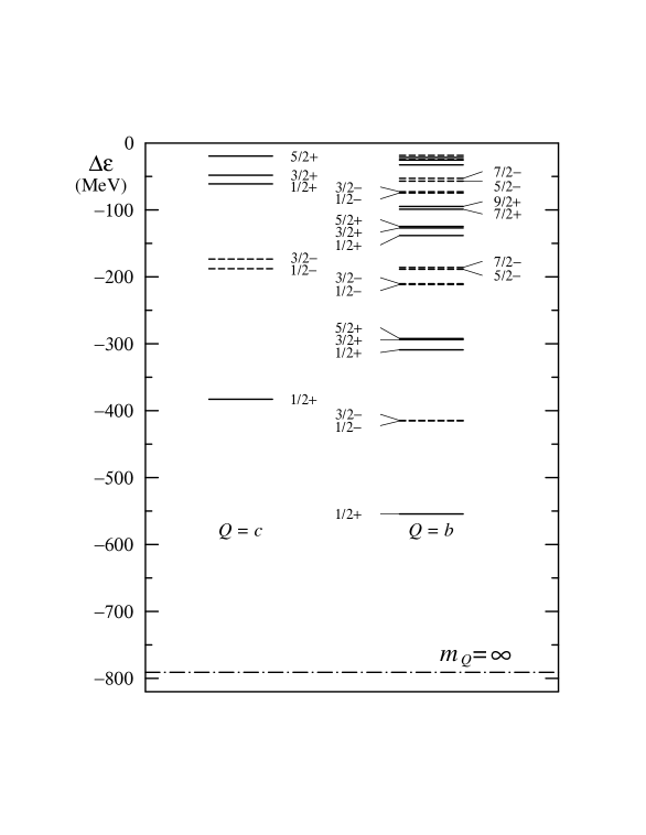
FIG. 1.: Energy levels of $k^{\pi}$ bound heavy meson states obtained with $f_{\pi}=64.5$ MeV, $e=5.45$, $m_{D}=1867$ MeV, $m_{D^{*}}=2010$ MeV, $m_{B}=5279$ MeV, $m_{B^{*}}=5325$ MeV, and $f_{Q}/2m_{\Phi^{*}}=g_{Q}=-0.75$. The dash-dotted line is the binding energy obtained in the infinite mass limit.

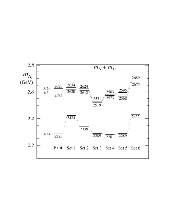
FIG. 2.: Parameter dependence of $\Lambda_{c}$ mass spectrum.

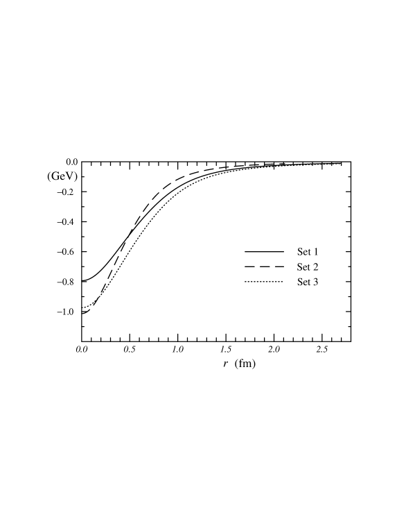
FIG. 3.: Shape of $\frac{1}{2}g_{Q}[a_{1}(r)-a_{2}(r)]$ with various parameter sets.

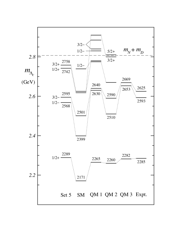
FIG. 4.: Mass spectrum of $\Lambda_{c}(j^{\pi})$. The results with Set 5 are presented. For a comparison, we use the experimental nucleon mass in Set 5. The predictions of other models, SM (Skyrme Model with only pseudoscalar heavy meson) [17], QM1 (Quark Model) [7], QM2 [8], and QM3 [9] are also given.

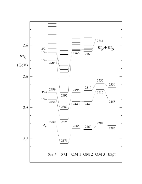
FIG. 5.: Mass spectrum of $\Sigma_{c}(j^{\pi})$. Notations are the same as in Fig. 4.

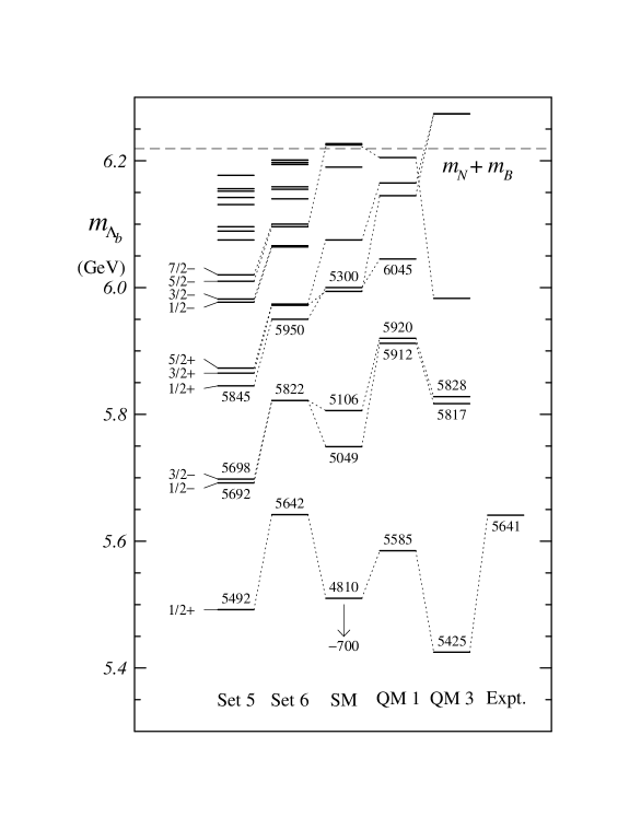
FIG. 6.: Mass spectrum of $\Lambda_{b}(j^{\pi})$. The predictions of Set 5 and Set 6 are presented with the results of SM [17], QM1 [7], and QM3 [9].

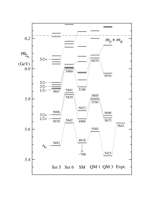
FIG. 7.: Mass spectrum of $\Sigma_{b}(j^{\pi})$. Notations are the same as in Fig. 6.

TABLE I.: Parameter sets. $f_{\pi}$ is in MeV unit and the others are dimensionless.

	$f_{\pi}$	$e$	$g_{Q}$	$f_{Q}/2m_{\Phi^{*}}$
Set 1	64.5	5.45	$-0.75$	$-0.75$
Set 2	93.0	4.82	$-0.75$	$-0.75$
Set 3	64.5	5.45	$-0.92$	$-0.92$
Set 4	93.0	4.82	$-0.81$	$-0.81$
Set 5	93.0	4.82	$-0.70$	$-0.85$
Set 6	93.0	4.82	$-0.65$	$-0.65$

REFERENCES

[1]
Particle Data Group, L. Montanet et al.,
Phys. Rev. D 50, 1173 (1994).
[2]
SKAT Collaboration, V. V. Ammosov et al.,
Pis’ma Zh. Eksp. Teor. Fiz. 58, 241 (1993)
[JETP Lett. 58, 247 (1993)].
[3]
ARGUS Collaboration, H. Albrecht et al.,
Phys. Lett. B 317, 227 (1993).
[4]
E687 Collaboration, P. L. Frabetti et al.,
Phys. Rev. Lett. 72, 961 (1994).
[5]
CLEO Collaboration, D. Acosta et al.,
in Lepton and Photon Interactions,
Proc. of the 16th International Symposium, Ithaca, New York,
1993, edited by P. Drell and D. Rubin (AIP, New York, 1994);
CLEO Collaboration, M. Battle et al.,
in Lepton and Photon Interactions,
Proc. of the 16th International Symposium, Ithaca, New York,
1993, op cit.
[6]
CLEO Collaboration, K. W. Edwards et al.,
Cornell Report No. CLNS-94-1304, 1994 (unpublished).
[7]
S. Capstick and N. Isgur,
Phys. Rev. D 34, 2809 (1986).
[8]
L. A. Copley, N. Isgur, and G. Karl,
Phys. Rev. D 20, 768 (1979).
[9]
C. S. Kalman and B. Tran,
Nuovo Cim. 102A, 835 (1989).
[10]
C. S. Kalman and D. Pfeffer,
Phys. Rev. D 27, 1648 (1983); 28, 2324 (1983).
[11]
K. Maltman and N. Isgur,
Phys. Rev. D 22, 1701 (1980).
[12]
J. L. Rosner,
University of Chicago Report No. EFL-95-02,
1995, hep-ph/9501291.
[13]
M. B. Voloshin and M. A. Shifman,
Yad. Fiz. 45, 463 (1987); 47, 801 (1988)
[Sov. J. Nucl. Phys. 45, 292 (1987);
47, 511 (1988)];
N. Isgur and M. B. Wise,
Phys. Lett. B 232, 113 (1989);
237, 527 (1990).
[14]
N. Isgur and M. B. Wise,
Phys. Rev. Lett. 66, 1130 (1991).
[15]
D. Izatt, C. Detar, and M. Stephenson,
Nucl. Phys. B199, 269 (1982).
[16]
P. Cho,
Phys. Rev. D 50, 3295 (1994).
[17]
M. Rho, D. O. Riska, and N. N. Scoccola,
Phys. Lett. B 251, 597 (1990);
Z. Phys. A 341, 343 (1992).
[18]
Y. Oh, B.-Y. Park, and D.-P. Min,
Phys. Rev. D 50, 3350 (1994).
[19]
C.-K. Chow and M. B. Wise,
Phys. Rev. D 50, 2135 (1994).
[20]
J. Schechter and A. Subbaraman,
Phys. Rev. D 51, 2311 (1995).
[21]
C. G. Callan and I. Klebanov,
Nucl. Phys. B262, 365 (1985).
[22]
E. Jenkins, A. V. Manohar, and M. B. Wise,
Nucl. Phys. B396, 27 (1993);
E. Jenkins and A. V. Manohar,
Phys. Lett. B 294, 273 (1992);
Z. Guralnik, M. Luke, and A. V. Manohar,
Nucl. Phys. B390, 474 (1993);
M. Nowak, M. Rho, and I. Zahed,
Phys. Lett. B 303, 130 (1993);
H. K. Lee and M. Rho,
Phys. Rev. D. 48, 2329 (1993);
K. S. Gupta, M. A. Momen, J. Schechter, and A. Subbaraman,
ibid.47, 4835 (1993);
A. Momen, J. Schechter, and A. Subbaraman,
ibid.49, 5970 (1994);
D.-P. Min, Y. Oh, B.-Y. Park, and M. Rho,
Int. Jour. Mod. Phys. E 4, 47 (1995).
[23]
K. Dannbom, E. M. Nyman, and D. O. Riska,
Phys. Lett. B 227, 291 (1989);
C. L. Schat, N. N. Scoccola, and C. Gobbi,
Nucl. Phys. A585, 627 (1995).
[24]
Y. Oh and B.-Y. Park,
Phys. Rev. D 51, 5016 (1995).
[25]
Y. Oh, B.-Y. Park, and D.-P. Min,
Phys. Rev. D 49, 4649 (1994).
[26]
J. Schechter, A. Subbaraman, S. Vaidya, and H. Weigel,
Nucl. Phys. A590, 655 (1995).
[27]
T.-M. Yan, H.-Y. Cheng, C.-Y. Cheung, G.-L. Lin,
Y. C. Lin, and H.-L. Yu,
Phys. Rev. D 46, 1148 (1992).
[28]
G. S. Adkins, C. R. Nappi, and E. Witten,
Nucl. Phys. B228, 552 (1983).
[29]
B. Moussalam and D. Kalafatis,
Phys. Lett. B 272, 196 (1991);
G. Holzwarth,
Nucl. Phys. A572, 69 (1994);
G. Holzwarth and H. Walliser,
ibid.A587, 721 (1995).
[30]
ACCMOR Collaboration, S. Barlag et al.,
Phys. Lett. B 278, 480 (1992);
CLEO Collaboration, S. Butler et al.,
Phys. Rev. Lett. 69, 2041 (1992).
[31]
R. Casalbuoni, A. Deandrea, N. Di Bartolomeo, R. Gotto,
F. Feruglio, and G. Nardulli,
Phys. Lett. B 292, 371 (1992); 299, 139 (1993);
P. Ko,
Phys. Rev. D 47, 1964 (1993);
J. Schechter and A. Subbaraman,
ibid.48, 332 (1993).
[32]
Y. Oh, B.-Y. Park, and D.-P. Min,
Phys. Lett. B 331, 362 (1994).
[33]
P. Colangelo, G. Nardulli, A. Deandrea, N. Di Bartolomeo, R. Gatto,
and F. Feruglio,
Phys. Lett. B 339, 151 (1994);
P. Jain, A. Momen, and J. Schechter,
Syracuse Report No. SU-4240-581, 1994, hep-ph/9406338.
[34]
A. De Rújula, H. Georgi, and S. L. Glashow,
Phys. Rev. D 12, 147 (1975).