The chiral phase transition in a random matrix model with molecular correlations

Abstract

The chiral phase transition of QCD is analyzed in a model combining random matrix elements of the Dirac operator with specially chosen non-random ones. The special form of the latter is motivated by the assumption that the fermionic quasi-zero modes associated with instanton and anti-instanton configurations determine the chiral properties of QCD. Our results show that the degree of correlation between these modes plays the decisive role. To reduce the value of the chiral condensate by more than a factor of 2 about 95 percent of the instantons and anti-instantons must form so-called molecules. This conclusion agrees with numerical results of the Stony Brook group.

, , and

One of the challenging tasks of hadron physics consists in understanding the properties of the chiral phase transition in QCD, and its relation to the deconfinement phase transition. This fascinating theoretical problem requires the consistent combination of several basic concepts of field theory: Dynamical and spontaneous symmetry breaking, non-trivial topological properties, confinement, and a hierarchy of correlation lengths. A deeper understanding of the chiral phase transition is also urgently required for the analysis of heavy ion collisions at very high energies. Such experiments will be done at RHIC and at LHC in the near future.

Because of its importance, this problem has received considerable theoretical attention especially during the last decade. Some papers which are particularly relevant for our investigation are listed in Refs. [1]–[14]. We use the notation of Shuryak, Verbaarschot, and Jackson [5, 7, 14] whose papers dominate the field. The derivation of the fundamental relations can be found there.

The starting point for most discussions is the Banks-Casher formula [15],

$$\langle\bar{q}q\rangle=-{\pi\over V_{4}}\rho(\mu)\Big{|}_{\mu=0}\;.$$ (1)

It links the value of the chiral condensate, $\langle\bar{q}q\rangle$, to the density of the eigenvalues $\mu$ of the Dirac equation,

$$\left(\mathrm{i}\partial/+g{\lambda^{a}\over 2}A/^{a}\right)\psi(x)=\mu\psi(x)\;,$$ (2)

at $\mu=0$. Here, $V_{4}$ is the four-volume, and $A^{a}$ the gluon field operator. The virtuality of typical fermion states is of order $\Lambda_{\mathrm{QCD}}$ so that they do not contribute to $\rho(0)$. This led to the assumption that $\rho(0)$ is dominated by very special states, the zero modes. Via the Atiyah-Singer index theorem,

$${g^{2}\over 32\pi^{2}}\epsilon_{\mu\nu\rho\sigma}~{}\int\d^{4}x~{}F^{a}_{\mu\nu}F^{a}_{\rho\sigma}=N_{+}-N_{-}\;,$$ (3)

these modes are linked to topologically non-trivial gauge field configurations (instantons and anti-instantons). Here, $N_{+}$ ($N_{-}$) is the number of zero modes with positive (negative) chirality. The integral on the left hand side contains the field tensor $F^{a}_{\mu\nu}$ and yields the topological charge $Q$. This charge is $+1$ ($-1$) for an isolated instanton (anti-instanton). To understand the behavior of the chiral condensate (and, thus, of hadron masses) as a function of, e.g., temperature $T$ it would then suffice to obtain the statistical properties of the zero modes associated with QCD-instantons. (For finite instanton separation, these are more precisely refered to as quasi-zero modes.) Some time ago, it was realized [5, 7] that at $T=0$, this statistical problem can be analyzed with the help of random matrix models; recently, this analysis was extended for the first time to finite temperature [14].

In this paper, we generalize these earlier contributions by investigating the dependence of the condensate on two parameters which characterize the temperature-dependence of the instanton configuration. One of these, $D$, is the strength of the (diagonal) interaction between fermionic states of opposite chirality. It is due to the formation of instanton–anti-instanton pairs (“molecules”) with an optimally attractive relative orientation in color space. This parameter was also used in Ref. [14]. The second parameter, $\alpha$, describes the fraction of instantons and anti-instantons which form such molecules. The inclusion of this new parameter is important because numerical simulations and phenomenological considerations suggest that it plays a crucial role in chiral symmetry breaking [8]. In some of our present work, we actually go beyond this simple two-parameter model and investigate distributions of the diagonal matrix elements. In this way, we derive some general statements about properties of the chiral phase transition, and about the associated critical exponents.

We see from Eq. (3) that each instanton or anti-instanton is associated with one quasi-zero mode. In any given sector of the theory, characterized by the value of the topological charge $Q=N_{+}-N_{-}$, the difference between the number of instantons and of anti-instantons is given by $Q$. In this sector, the QCD partition function for a theory with $N_{f}$ fermionic flavors is thus approximated by

$$Z_{\mathrm{QCD}}(Q)=\lim_{N_{\pm}\rightarrow\infty}\left\langle\prod_{f=1}^{N_{f}}\det\left(\mathrm{i}\partial/+g{\lambda^{a}\over 2}A/^{a}+\mathrm{i}m_{f}\right)\right\rangle_{A}\;.$$ (4)

Here, only quasi-zero modes are taken into account; the matrix in (4) accordingly has dimension $(2N+Q)$. (We define $N=N_{-}$ and assume without loss of generality that $Q\geq 0$.) The average in (4) extends over all gauge field configurations $A^{a}$ with topological charge $Q$ and the usual measure. The symbol $m_{f}$ denotes the mass term.

In a basis of chirality eigenstates, the operator $\mathrm{i}\partial/+g{\lambda^{a}\over 2}A/^{a}$ couples fields of different chirality while the mass term in the determinant conserves chirality. The determinant can be rearranged so that the first $(N+Q)$ states have positive chirality and are localized at the $(N+Q)$ instanton positions, while the remaining $N$ states are the quasi-zero states with negative chirality and are localized at the anti-instanton positions. This yields

$$\det\left(\matrix{\mathrm{i}m_{f}&\mathrm{i}\partial/+g{\lambda^{a}\over 2}A/^{a}\cr(\mathrm{i}\partial/+g{\lambda^{a}\over 2}A/^{a})^{\dagger}&\mathrm{i}m_{f}}\right)\;.$$ (5)

The chirality-changing matrix elements have the form

$$\phi^{*}_{I_{k}}\left(\mathrm{i}\!\!\stackrel{{\scriptstyle\rightarrow}}{{\partial/}}+g{\lambda^{a}\over 2}A/^{a}(I_{k})+g{\lambda^{a}\over 2}A/^{a}(\bar{I}_{l})+\sum_{j\neq k,l}g{\lambda^{a}\over 2}A/^{a}(j)+g{\lambda^{a}\over 2}A/^{a}_{\mathrm{fluct}}\right)\phi_{\bar{I}_{l}}$$ (6)

$$=\phi^{*}_{I_{k}}\left(g{\lambda^{a}\over 2}A/^{a}(I_{k})+\sum_{j\neq k,l}g{\lambda^{a}\over 2}A/^{a}(j)+g{\lambda^{a}\over 2}A/^{a}_{\mathrm{fluct}}\right)\phi_{\bar{I}_{l}}$$

$$=\phi^{*}_{I_{k}}\left(-\mathrm{i}\!\!\stackrel{{\scriptstyle\leftarrow}}{{\partial/}}+\sum_{j\neq k,l}g{\lambda^{a}\over 2}A/^{a}(j)+g{\lambda^{a}\over 2}A/^{a}_{\mathrm{fluct}}\right)\phi_{\bar{I}_{l}}\;.$$

Here, we have assumed that the $\phi_{I_{k}}$ ($\phi_{\bar{I}_{l}}$) are exact zero modes of the Dirac operator when the gauge field $A^{a}$ in Eq. (2) is replaced by the field $A^{a}(I_{k})$ [$A^{a}(\bar{I}_{l})$] due to a single instanton (anti-instanton). It is assumed that these instantons and anti-instantons differ and are well separated, with uncorrelated color orientation. The symbol $A^{a}_{\mathrm{fluct}}$ denotes the fluctuating part of the gauge field not linked to specific instanton configurations. The matrix elements in the last line of Eq. (6) can be replaced by the elements of a random matrix with suitable symmetry properties [5, 7, 14]. This leads to a random-matrix model with partition function

$$Z_{\beta}(Q)=\int{\cal D}[W] \exp\left[-\frac{N\beta\Sigma^{2}}{2}\mathrm{tr}(WW^{\dagger})\right]$$ (7)

$$\times\prod_{f=1}^{N_{f}}\det\left(\matrix{m_{f}&\mathrm{i}W\!+\!\mathrm{i}D\cr\mathrm{i}W^{\dagger}\!+\!\mathrm{i}D^{\dagger}&m_{f}}\right)\;.$$

The matrix $W$ is a rectangular matrix with $(N+Q)$ rows and $N$ columns. Depending on the underlying symmetry, we distinguish three random matrix ensembles pertaining to the partition function (7), labeled by $\beta=1$, 2, and 4: the Gaussian orthogonal ensemble (GOE, $\beta=1$), the Gaussian unitary ensemble (GUE, $\beta=2$), and the Gaussian symplectic ensemble (GSE, $\beta=4$) with real, complex, or quaternion real matrices $W$, respectively. As shown by Verbaarschot [7], these three cases correspond to the following gauge groups: SU(2) in the fundamental representation for $\beta=1$, SU($N_{c}$) with $N_{c}\geq 3$ in the fundamental representation for $\beta=2$, and non-Abelian gauge groups SU($N_{c}$) for all $N_{c}$ with fermions in the adjoint representation for $\beta=4$. In this letter, we are concerned with the case $\beta=2$ only. The integration measure in Eq. (7) is the Haar measure. The parameter $\Sigma$ is a real number which is related to the value of the condensate at $T=0$ and which we take to be independent of temperature. Lattice calculations [10] suggest that $\Sigma$ can depend on temperature only weakly; such a dependence cannot affect our results qualitatively.

The matrix $D$ is real and diagonal. As mentioned above, $D$ is included to describe the non-random components of the Dirac matrix elements due to the formation of instanton–anti-instanton pairs with an optimally attractive relative orientation in color space. The matrix $D$ is diagonal because only the two quasi-zero modes of opposite chirality belonging to such a pair are coupled by a non-random matrix element. We expect the elements of $D$ to grow with increasing temperature. This point will be substantiated below. The $T$-dependence of $D$ generates the $T$-dependence of the chiral condensate. In the sequel, we study several distributions of the matrix elements of $D$. Analytical results are obtained only for the simplest of these, for which a fraction $\alpha$ of the elements of $D$ is non-zero, all non-zero elements being equal. We believe that the distributions we study should account for the most important features of QCD related to the chiral phase transition, with one possible proviso. It would seem much more realistic to replace the random matrix $W$ by a banded random matrix [16]. This would account for the fact that the interaction of widely separated zero modes should be suppressed, and would introduce a correlation length in the theory. Work on this problem is under way.

We turn to the details of the calculation. The determinant in (7) can be rewritten as an integral over anti-commuting (Grassmann) variables [17],

$$Z_{2}(Q)=\int{\cal D}[W]{\cal D}[\psi]\exp\Bigg{[}\!\! -\sum_{f=1}^{N_{f}}\psi^{f*}\left(\matrix{m_{f}&\mathrm{i}W\!+\!\mathrm{i}D\cr\mathrm{i}W^{\dagger}\!+\!\mathrm{i}D^{\dagger}&m_{f}}\right)\psi^{f}$$ (8)

$$-N\Sigma^{2}\mathrm{tr}(WW^{\dagger})\Bigg{]}\;.$$

The (anti-commuting) vector $\psi$ has $N_{f}\,(2N+Q)$ components which we label as follows. The upper index $f\!=\!1\ldots N_{f}$ denotes the flavor, and the lower index numbers the (anti-) instanton zero modes. The first $N+Q$ components of the lower index denote the instanton zero modes labeled by $I_{k}$ with $k\!=\!1\ldots N+Q$, and the remaining $N$ components the anti-instanton zero modes labeled by $\bar{I}_{l}$ with $l\!=\!1\ldots N$. Performing the integration over $W$ we obtain

$$Z_{2}(Q)=\int{\cal D}[\psi]\exp\Biggl{[}\!\! \frac{1}{N\Sigma^{2}}\psi_{{\bar{I}}_{l}}^{f*}\psi_{{\bar{I}}_{l}}^{g}\psi_{I_{k}}^{g*}\psi_{I_{k}}^{f}-m_{f}(\psi_{I_{k}}^{f*}\psi_{I_{k}}^{f}+\psi_{{\bar{I}}_{l}}^{f*}\psi_{{\bar{I}}_{l}}^{f})$$ (9)

$$-\mathrm{i}D_{l}(\psi_{I_{l}}^{f*}\psi_{{\bar{I}}_{l}}^{f}+\psi_{{\bar{I}}_{l}}^{f*}\psi_{I_{l}}^{f})\Biggr{]}\;.$$

Summation over repeated indices is assumed, and we have set $D_{ll}=D_{l}$. The four-fermion terms can be removed by means of a Hubbard-Stratonovitch transformation at the expense of introducing $2N_{f}^{2}$ additional integration variables. These can be taken to be the elements of a complex $N_{f}\times N_{f}$ matrix $S$. The result can be rearranged as

$$Z_{2}(Q)=\int{\cal D}[S]{\cal D}[\psi]\exp\Biggl{[}\!\! -N\Sigma^{2}\mathrm{tr}(SS^{\dagger})-\sum_{k=N+1}^{N+Q}\psi_{I_{k}}^{*}(S+M)\psi_{I_{k}}$$ (10)

$$-\sum_{k=1}^{N}\left(\matrix{\psi_{I_{k}}^{*}\cr\psi_{\bar{I}_{k}}^{*}}\right)\left(\matrix{S+M&\mathrm{i}D_{k}\cr\mathrm{i}D_{k}&S^{\dagger}+M}\right)\left(\matrix{\psi_{I_{k}}\cr\psi_{\bar{I}_{k}}}\right)\Biggr{]}\;,$$

where the $\psi$-vectors are now in flavor space, the $D_{k}$ are multiplied by the $N_{f}\times N_{f}$ unit matrix, and the matrix $M$ is a diagonal matrix with entries $m_{f}$. The integration over the Grassmann variables can now be performed to yield

$$Z_{2}(Q)=\int{\cal D}[S] \exp\left[-N\Sigma^{2}\mathrm{tr}(SS^{\dagger})\right]{\det}^{Q}(S+M)$$ (11)

$$\times\prod_{k=1}^{N}\det\left(\matrix{S+M&\mathrm{i}D_{k}\cr\mathrm{i}D_{k}&S^{\dagger}+M}\right)\;.$$

The $\langle\bar{q}q\rangle$-condensate is given by

$$\langle\bar{q}q\rangle=\frac{1}{V_{4}N_{f}}\left.\frac{\partial\log Z}{\partial M}\right|_{M=0}$$ (12)

which, using (11), can be expressed as

$$\langle\bar{q}q\rangle=\int{\cal D}[S] \exp\left[-N\Sigma^{2}\mathrm{tr}(SS^{\dagger})\right]{\det}^{Q}(S)\prod_{k=1}^{N}\det\left(\matrix{S&\mathrm{i}D_{k}\cr\mathrm{i}D_{k}&S^{\dagger}}\right)$$ (13)

$$\times\frac{1}{V_{4}N_{f}}\left\{Q\mathrm{tr}(S^{-1})+\sum_{k=1}^{N}\mathrm{tr}\left(\matrix{S&\mathrm{i}D_{k}\cr\mathrm{i}D_{k}&S^{\dagger}}\right)^{-1}\right\}\;.$$

In the limit $N\rightarrow\infty$, the integral in (11) can be evaluated in saddle-point approximation. Neglecting terms of order $Q$, we obtain

$$N\Sigma^{2}S=\sum_{k=1}^{N}(S+M)\left[(S+M)(S^{\dagger}+M)+D_{k}^{2}\right]^{-1}\;.$$ (14)

Any square complex matrix of dimension $N_{f}$ can be written as $S=U\Lambda V^{-1}$, where $\Lambda$ is a diagonal matrix with real and non-negative entries, $U$ is unitary, and $V\!\in\!\mathrm{U}(N_{f})/\bigotimes_{n=1}^{N_{f}}\mathrm{U}(1)$. The solution of (14) in the limit of zero masses is, thus, obtained by solving

$$\Sigma^{2}=\frac{1}{N}\sum_{k=1}^{N}\frac{1}{\lambda^{2}+D_{k}^{2}}$$ (15)

for $\lambda$. The $\langle\bar{q}q\rangle$-condensate then follows from Eq. (13),

$$\langle\bar{q}q\rangle=\Sigma^{2}\lambda{2N+Q\over V_{4}}=\Sigma^{2}\lambda n_{\rm inst}\;,$$ (16)

where $n_{\rm inst}$ is the instanton–anti-instanton density.

In a realistic physical situation, the entries $D_{k}$ are distributed according to some (normalized) distribution $P(D_{k})$. In the limit $N\rightarrow\infty$, we can map the (discrete) interval $k\!=\!1\ldots N$ onto the (continuous) interval $x\!=\!0\ldots 1$. The desired value of $\lambda$ is then obtained by solving the equation

$$\Sigma^{2}=\int_{0}^{1}\frac{\d x}{\lambda^{2}+D^{2}(x)}$$ (17)

for $\lambda$. Here, $D(x)$ is defined by

$$\int_{0}^{D(x)}P(y)\d y=x\;.$$ (18)

Although the above equations cannot in general be solved analytically one can still make interesting statements about the connection between the existence of a condensate and the analytical form of $P(y)$ for small $y$. A condensate exists if Eq. (17) has a positive solution for $\lambda$. This is the case if $\int_{0}^{1}\d x/D^{2}(x)>\Sigma^{2}$. Since $D(x)$ increases monotonically by definition this condition is automatically fulfilled if $D(x)\sim x^{a}$ for small $x$ with $a\geq 1/2$. Using Eq. (18), this is equivalent to $P(y)\sim y^{b}$ for small $y$ with $b\leq 1$. The distribution $P$ is a function of temperature. Hence, necessary conditions for the vanishing of the condensate above some critical temperature $T_{\mathrm{c}}$ are

$$P(y)\sim y^{b}\ \ \mathrm{for}\ \ y\rightarrow 0\ \ \mathrm{with}\ \ b>1$$ (19)

$$\int_{0}^{1}\frac{\d x}{D^{2}(x)}\leq\Sigma^{2}\;.$$ (20)

While these conditions set non-trivial constraints on the general distribution of the diagonal elements, it is more convenient for our purposes to consider a number of interesting special cases where analytical results can be obtained. The simplest possible case is that where all elements of $D$ are equal, corresponding to $P(y)=\delta(y-d)$ and $D(x)=d$. The solution for $\lambda$ can be obtained immediately to yield

$$\langle\bar{q}q\rangle=\Sigma n_{\rm inst}\sqrt{1-(\Sigma d)^{2}}\;.$$ (21)

This version of the model with $d=\pi T$ was considered by Jackson and Verbaarschot [14].

As a more realistic case we assume that a fraction $\alpha\in[0,1]$ of the elements of $D$ are equal to a common value $d$ and the remaining elements are zero. This corresponds to $P(y)=\alpha\delta(y-d)+(1-\alpha)\delta(y)$, $D(x)=0$ for $0<x<1-\alpha$, and $D(x)=d$ for $1-\alpha<x<1$. Again, we can solve for $\lambda$ to obtain

$$\langle\bar{q}q\rangle=\frac{\Sigma n_{\rm inst}}{\sqrt{2}}\sqrt{1-(\Sigma d)^{2}+\sqrt{[1-(\Sigma d)^{2}]^{2}+4(\Sigma d)^{2}(1-\alpha)}}\;.$$ (22)

This result is shown graphically in Fig. 1. Its most important property is that $\langle\bar{q}q\rangle$ can approach zero only if $\alpha$ is very close to one. This observation is in striking agreement with the results of a specific model by Ilgenfritz and Shuryak [8] and with the general observation that the chiral condensate changes abruptly at the chiral phase transition [11] while the instanton density changes only very smoothly. Note also that the relatively sharp drop of the chiral condensate close to the critical temperature is in qualitative agreement with results obtained by the Bern Group in the framework of chiral perturbation theory [18]. We conclude from our results that this is a generic property which follows from the symmetries of the interaction and the fundamental properties of instanton molecules. Thus, any specific model should reproduce these features.

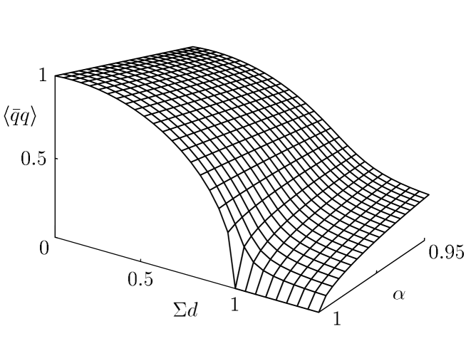
Figure 1: Plot of the $\langle\bar{q}q\rangle$ condensate in units of its value at $T=0$ as a function of $d$ and $\alpha$ defined in the text. Both $d$ and $\alpha$ are functions of temperature so that the dependence of $\langle\bar{q}q\rangle$ on $T$ corresponds to a specific path on this surface.

At this point, we are in a position to discuss specific numbers corresponding to the real physical situation. The QCD vacuum state is characterized by a number of quantities, one of them being the gluon condensate $\langle{\alpha\over\pi}G^{a}_{\mu\nu}G^{a}_{\mu\nu}\rangle$, which in turn can be related to the instanton–anti-instanton density (in Euclidean space-time). Phenomenologically, $n_{\rm inst}\approx$ 1 fm^-4 at $T=0$. It is expected [8] that this value changes only little with temperature up to $T_{\mathrm{c}}$. The typical instanton radius $\rho$ is equal to the color correlation length which is determined by many phenomenological considerations (e.g., from pomeron phenomenology or from the gluon form factor [19]) to be about 0.3 fm at $T=0$. The same number is determined by fitting a host of hadronic properties in the instanton vacuum model of Shuryak and co-workers. These numbers are further corroborated by specialized lattice studies using cooling techniques to single out the quasi-classical field configurations [20, 21]. Furthermore, the separation of instanton and anti-instanton in a correlated pair is $R\approx$ 1 fm [20], and the empirical value of the quark condensate is $\langle\bar{q}q\rangle\approx-$(225 MeV)³ [22].

The diagonal matrix elements $d$ have been calculated by Diakonov and Petrov [2], Eq. (22). For an optimally attractive orientation of instanton and anti-instanton this implies

$$|d|={4\rho^{2}\over R^{3}}\approx 0.4~{}{\rm fm}^{-1}$$ (23)

at $T=0$. On the other hand, we have for the ground state with no noticeable instanton-anti-instanton correlation ($\alpha\rightarrow 0$)

$$\Sigma=\left.{\langle\bar{q}q\rangle\over n_{\rm inst}}\right|_{T=0}\approx-1.5~{}{\rm fm}\;.$$ (24)

These numbers imply $\sqrt{1-(\Sigma d)^{2}}\approx 0.8$ at $T=0$. Thus, it is not sufficient that $\alpha$ approaches one, but in addition $d$ has to increase by about fifty percent as $T$ increases from zero to $T_{\rm c}$. This can be achieved by an increase of $\rho$ and/or a decrease of $R$. Lattice studies indicate that $\rho$ is approximately independent of $T$ [21]. Recent calculations by T. Schäfer and E. Shuryak in the framework of the instanton liquid model show that $R$ decreases with $T$ [23]. Thus, an overall inrease of $d$ with temperature is plausible.

We can compute various critical exponents from the above results. Our order parameter is $\langle\bar{q}q\rangle$, and the control parameter is the temperature $T$. Let us concentrate on Eq. (22). The two parameters $d$ and $\alpha$ depend on $T$ in a way which is beyond the scope of our model. However, some qualitative statements can be made on physical grounds. At $T=0$, $d$ has some finite value whereas $\alpha$ is zero. Both parameters will grow with temperature, but $\alpha$ is bounded by one. It is reasonable to assume that $d$ is an analytic function of $T$, but no such assumption can be made for the behavior of $\alpha(T)$ close to $\alpha=1$. There is even the possibility that $\alpha$ changes discontinuously to one resulting in a first order transition. We note that our model is rich enough to allow for that possibility but will assume in the following discussion that $\alpha$ is a continuous though not necessarily analytic function of $T$.

It is clear from Eq. (22) and Fig. 1 that necessary conditions for a vanishing condensate are $\Sigma d\geq 1$ and $\alpha=1$. Let us denote the temperatures at which these two conditions are first satisfied by $T_{d}$ and $T_{\alpha}$, respectively. The larger of these two temperatures is the critical temperature $T_{\mathrm{c}}$, but we do not know a priori which one it will be. In principle, there are three possibilities: (i) $T_{\mathrm{c}}=T_{d}>T_{\alpha}$, (ii) $T_{\mathrm{c}}=T_{d}=T_{\alpha}$, and (iii) $T_{\mathrm{c}}=T_{\alpha}>T_{d}$. We are interested in the critical exponent $\beta$ defined by

$$\langle\bar{q}q\rangle\sim|t|^{\beta}\ \ \mathrm{with}\ \ t=\frac{T-T_{\mathrm{c}}}{T_{\mathrm{c}}}\;.$$ (25)

(This $\beta$ is, of course, different from the $\beta$ labeling the random matrix ensembles.) For cases (ii) and (iii), $\beta$ depends on the specific form of $\alpha(T)$ close to $T_{\alpha}$. We parameterize this dependence by $1-\alpha(t)\sim|t|^{x}$ for $t\rightarrow 0^{-}$. We then obtain for case (i) $\beta={\textstyle\frac{1}{2}}$, for case (ii) $\beta={\textstyle\frac{1}{2}}$ for $x\geq 2$ and $\beta=\frac{x}{4}$ for $x<2$, and for case (iii) $\beta=\frac{x}{2}$.

The critical exponents $\gamma$ and $\delta$ are defined by

$$\chi\sim|t|^{-\gamma}\ \ \mathrm{with}\ \ \chi\sim\left.\frac{\partial\langle\bar{q}q\rangle}{\partial m}\right|_{m=0}$$ (26)

$$\langle\bar{q}q\rangle\sim m^{1/\delta}\ \ \mathrm{at}\ \ T=T_{\mathrm{c}}\;.$$ (27)

In this case, the mass $m$ plays the role of the conjugate field breaking chiral symmetry explicitly (the analog of the external magnetic field in the case of a ferromagnet). Both $\gamma$ and $\delta$ can be computed in a straightforward manner by going back to Eq. (14). The results, however, again depend on the relationship between $T_{d}$ and $T_{\alpha}$. We find that in case (i) $\gamma=1$ both above and below the transition and $\delta=3$ in agreement with Ref. [14]. In case (iii) $\gamma=0$ both above and below the transition and $\delta=1$. Case (ii) is more complicated. We obtain that above the transition $\gamma=1$ whereas below the transition $\gamma=1$ for $x\geq 2$ and $\gamma=\frac{x}{2}$ for $x<2$. Furthermore, $\delta=3$ here. In all three cases, the Widom scaling law, $\gamma=\beta(\delta-1)$, is obeyed.

Case (i) and case (ii) for $x\geq 2$ yield the standard mean-field exponents while case (ii) for $x<2$ and case (iii) give rise to critical exponents which do not seem to be in a familiar universality class. This finding deserves further discussion.

When considering a second order phase transition, one usually assumes that the “input” parameters of the system (in our case, $d$ and $\alpha$) depend on the control parameter in a smooth and analytic way. The non-analytic features of the “output” parameters (e.g., the order parameter) at the critical temperature are a consequence of the phase transition. It is not in the spirit of such considerations to introduce non-analyticities at the outset, i.e., in the input parameters. In our specific case, we are not able to specify how $\alpha$ approaches one as $T\rightarrow T_{\alpha}^{-}$. However, $\alpha$ is special in the sense that it is strictly equal to one for $T>T_{\alpha}$. Thus, requiring $\alpha(T)$ to be continuous and differentiable at $T_{\alpha}$ yields $1-\alpha(T)\sim(T_{\alpha}-T)^{2}$ for $T\rightarrow T_{\alpha}^{-}$ and, hence, $x=2$ in the above results for $\beta$ and $\gamma$. Therefore, if it should turn out that either $T_{d}>T_{\alpha}$ or $T_{d}=T_{\alpha}$ with $\alpha(T)$ continuous and differentiable at $T_{\alpha}$, we reproduce the mean field exponents of a second order phase transition. This would be consistent with the recent discussion in [24]. If $T_{d}<T_{\alpha}$ or $T_{d}=T_{\alpha}$ with $\alpha(T)$ continuous but not differentiable at $T_{\alpha}$, we obtain a second order phase transition with non-standard critical exponents. Finally, if $\alpha$ is discontinuous at $T_{\alpha}\geq T_{d}$, we obtain a first order transition.

In summary, we have extended the chiral random-matrix model of Refs. [5, 7, 14] in such a way that the model allows either for a first-order or for a second-order chiral phase transition. For the second-order transition, we have calculated the critical exponents, and we found a number of possible solutions, all consistent with universal scaling laws. A decision between them is beyond the present scope of our model. We believe, however, that these options define the generic possibilities of any physically realistic model of the chiral phase transition.

We would like to thank A. D. Jackson and J. J. M. Verbaarschot for communicating their results prior to publication and useful discussions. TW also acknowledges helpful discussions with T. Guhr, T. Schäfer, and E. V. Shuryak. AS thanks D. Diakonov for very valuable discussions and the MPI für Kernphysik, Heidelberg, as well as the ECT^∗, Trento, for its support.

References

- [1] D. I. Diakonov and V. Yu. Petrov, Phys. Lett. B 147 (1984) 351; Nucl. Phys. B 245 (1984) 259; Sov. Phys. JETP 62 (1985) 204, 431.
- [2] D. I. Diakonov and V. Yu. Petrov, Nucl. Phys. B 272 (1986) 457.
- [3] D. I. Diakonov and A. D. Mirlin, Phys. Lett. B 203 (1988) 2991.
- [4] Yu. A. Simonov, Sov. J. Nucl. Phys. 53 (1991) 1099; Phys. Rev. D 43 (1991) 3534.
- [5] E. Shuryak and J. Verbaarschot, Nucl. Phys. A 560 (1993) 306; Nucl. Phys. B 341 (1990) 1; Phys. Rev. Lett. 68 (1992) 2576.
- [6] J. Verbaarschot, Nucl. Phys. B 427 (1994) 534.
- [7] J. J. M. Verbaarschot, Phys. Rev. Lett. 72 (1994) 2531.
- [8] E.-M. Ilgenfritz and E. V. Shuryak, Phys. Lett. B 325 (1994) 263.
- [9] T. Schäfer, E. V. Shuryak, and J. J. M. Verbaarschot, Phys. Rev. D 51 (1995) 1267.
- [10] A. DiGiacomo, E. Meggiolaro, and H. Panagopoulos, Phys. Lett. B 277 (1992) 491.
- [11] F. Karsch, XI. Conference on Ultra-Relativistic Nucleus-Nucleus-Collisions, Monterey 1995, USA, preprint BI-TP 95/11, hep-lat/9503010 (1995).
- [12] C. F. Baillie et al., Phys. Lett. B 197 (1987) 195.
- [13] G. Bunatian and J. Wambach, Phys. Lett. B 336 (1994) 290.
- [14] A. D. Jackson and J. J. M. Verbaarschot, preprint hep-ph/9509324 (1995).
- [15] T. Banks and A. Casher, Nucl. Phys. B 169 (1980) 103.
- [16] Y. V. Fyodorov and A. D. Mirlin, Phys. Rev. Lett. 67, 2405 (1991).
- [17] J. J. M. Verbaarschot, H. A. Weidenmüller, and M. Zirnbauer, Phys. Rep. 129 (1985) 367.
- [18] J. Gasser and H. Leutwyler, Phys. Lett. B 188, 477 (1987).
- [19] V. M. Braun, P. Gornicki, L. Mankiewicz, and A. Schäfer, Phys. Lett. B 302 (1993) 291.
- [20] M.-C. Chu, J. M. Grandy, S. Huang, and J. W. Negele, Phys. Rev. D 49 (1994) 6039; D. I. Diakonov, “Instanton vacuum and confinement in QCD”, Third St. Petersburg Winter School in QCD, Feb. 26–Mar. 11, 1995.
- [21] M.-C. Chu and S. Schramm, Phys. Rev. D 51 (1995) 4580.
- [22] L. J. Reinders, H. Rubinstein, and S. Yazaki, Phys. Rep. 127, 1 (1985).
- [23] T. Schäfer and E. V. Shuryak, preprint hep-ph/9509337 (1995).
- [24] A. Kocić and J. Kogut, Phys. Rev. Lett. 74 (1995) 3109.