PROPERTIES OF THE STRANGE AXIAL MESONS
IN THE RELATIVIZED QUARK MODEL

Abstract

We studied properties of the strange axial mesons in the relativized quark model. We calculated the $K_{1}$ decay constant in the quark model and showed how it can be used to extract the $K_{1}(^{3}P_{1})-K_{1}(^{1}P_{1})$ mixing angle ($\theta_{K}$) from the weak decay $\tau\to K_{1}\nu_{\tau}$. The ratio $BR(\tau\to\nu_{\tau}K_{1}(1270))/BR(\tau\to\nu_{\tau}K_{1}(1400))$ is the most sensitive measurement and also the most reliable since the largest of the theoretical uncertainties factor out. However the current bounds extracted from the TPC/Two-Gamma collaboration measurements are rather weak: we typically obtain $-30^{o}\lesssim\theta_{K}\lesssim 50^{o}$ at 68% C.L. We also calculated the strong OZI-allowed decays in the pseudoscalar emission model and the flux-tube breaking model and extracted a ${}^{3}P_{1}-^{1}P_{1}$ mixing angle of $\theta_{K}\simeq 45^{o}$. Our analysis also indicates that the heavy quark limit does not give a good description of the strange mesons.

I INTRODUCTION

The strange axial mesons offer interesting possibilities for the study of QCD in the non-perturbative regime through the mixing of the ${}^{3}P_{1}$ and ${}^{1}P_{1}$ states. In the SU(3) limit these states do not mix, just as the $a_{1}$ and $b_{1}$ mesons do not mix. For a strange quark mass greater than the up and down quark masses SU(3) is broken so that the ${}^{3}P_{1}$ and ${}^{1}P_{1}$ states mix to give the physical $K_{1}$ states. In the heavy quark limit where the strange quark becomes infinitely heavy, the light quark’s spin couples with the orbital angular momentum resulting in the light quark having total angular momentum $j={3\over 2}$ in one state and $j={1\over 2}$ in the other state, each state having distinct properties[1, 2, 3]. By studying the strange axial mesons and comparing them to the heavy quark limit one might gain some insights about hadronic properties in the soft QCD regime.

Recently, the TPC/Two-Gamma Collaboration has presented measurements for the decays $\tau^{-}\to\nu_{\tau}K_{1}^{-}(1270)$ and $\tau^{-}\to\nu_{\tau}K_{1}^{-}(1400)$ [4]. It is expected that the LEP, CLEO, and BES collaborations, with their large samples of $\tau$’s, will be able to study these decays in further detail [5]. These decays provide another means of studying ${}^{3}P_{1}-^{1}P_{1}$ mixing of the strange axial mesons in addition to using their partial decay widths and masses.

In this paper we study the properties of the strange axial mesons in the context of the relativized quark model [6, 7]. We compare the experimental measurements to the predictions of the model to extract the ${}^{3}P_{1}-^{1}P_{1}$ mixing angle ($\theta_{K}$). Comparing both the experimental measurements and model results to various limits helps in understanding the nature of QCD in the soft regime.

We begin in Sec. II with a brief description of the relativized quark model and a description of the ${}^{3}P_{1}-^{1}P_{1}$ mixing. By comparing the mass predictions of the quark model to the observed $K_{1}$ masses we obtain our first estimate for $\theta_{K}$. In Sec. III we calculate the $K_{1}$ decay constants using the mock-meson approach and use the results to obtain a second estimate of $\theta_{K}$. In Sec. IV we study the strong decay properties of these states using the pseudoscalar emission model[6] and the flux-tube breaking model [8] and use the results as another way of measuring the ${}^{3}P_{1}-^{1}P_{1}$ mixing angle. When appropriate we examine the non-relativistic and heavy quark limits to gain insights into the underlying dynamics. Various aspects of the phenomenology of the strange axial mesons have also been studied by Suzuki in a series of recent papers [9, 10] using approaches complementary to ours.

II THE $K_{1}$ MASSES and ${}^{3}P_{1}-^{1}P_{1}$ MIXING

In this section we give a very brief description of the relativized quark model [6, 7]. The spin-orbit contributions in particular will be important in understanding the ${}^{3}P_{1}-^{1}P_{1}$ mixing. The model is not derived from first principles but rather is motivated by expected relativistic properties. Although progress is being made using more rigorous approaches, the relativized quark model describes the properties of hadrons reasonably well and presents an approach which can give insights into the underlying dynamics that can be obscured in the more rigorous approaches.

The basic equation of the model is the rest frame Schrödinger-type equation. The effective potential, $V_{q\bar{q}}(\vec{p},\vec{r})$, is described by a Lorentz-vector one-gluon-exchange interaction at short distances and a Lorentz-scalar linear confining interaction. $V_{q\bar{q}}(\vec{p},\vec{r})$ was found by equating the scattering amplitude of free quarks, using a scattering kernel with the desired Dirac structure, with the effects between bound quarks inside a hadron [11]. Due to relativistic effects the potential is momentum dependent in addition to being co-ordinate dependent. The details of the model can be found in Ref. [6]. To first order in $(v/c)^{2}$, $V_{q\bar{q}}(\vec{p},\vec{r})$ reduces to the standard non-relativistic result:

$$V_{q\bar{q}}(\vec{p},\vec{r})\to V(\vec{r})=H^{conf}_{q\bar{q}}+H^{cont}_{q\bar{q}}+H^{ten}_{q\bar{q}}+H^{s.o.}_{q\bar{q}}$$ (1)

where

$$H^{conf}_{q\bar{q}}=C+br+{{\alpha_{s}(r)}\over r}\vec{F}_{q}\cdot\vec{F}_{\bar{q}}$$ (2)

includes the spin-independent linear confinement and Coulomb-like interaction,

$$H^{cont}_{q\bar{q}}=-{{8\pi}\over 3}{{\alpha_{s}(r)}\over{m_{q}m_{\bar{q}}}}\vec{S}_{q}\cdot\vec{S}_{\bar{q}}\delta^{3}(\vec{r})\;\vec{F}_{q}\cdot\vec{F}_{\bar{q}}$$ (3)

is the colour contact interaction,

$$H^{ten}_{q\bar{q}}=-{{\alpha_{s}(r)}\over{m_{q}m_{\bar{q}}}}{1\over{r^{3}}}\left[{{{3\vec{S}_{q}\cdot\vec{r}\;\vec{S}_{\bar{q}}\cdot\vec{r}}\over{r^{2}}}-\vec{S}_{q}\cdot\vec{S}_{\bar{q}}}\right]\;\;\vec{F}_{q}\cdot\vec{F}_{\bar{q}}$$ (4)

is the colour tensor interaction,

$$H^{s.o.}_{q\bar{q}}=H^{s.o.(cm)}_{q\bar{q}}+H^{s.o.(tp)}_{q\bar{q}}$$ (5)

is the spin-orbit interaction with

$$H^{s.o.(cm)}_{q\bar{q}}=-{{\alpha_{s}(r)}\over{r^{3}}}\left({{{\vec{S}_{q}}\over{m_{q}m_{\bar{q}}}}+{{\vec{S}_{\bar{q}}}\over{m_{q}m_{\bar{q}}}}+{{\vec{S}_{q}}\over{m_{q}^{2}}}+{{\vec{S}_{\bar{q}}}\over{m_{\bar{q}}^{2}}}}\right)\cdot\vec{L}\;\vec{F}_{q}\cdot\vec{F}_{\bar{q}}$$ (6)

its colour magnetic piece arising from one-gluon exchange and

$$H^{s.o.(tp)}_{q\bar{q}}=-{1\over{2r}}{{\partial H_{q\bar{q}}^{conf}}\over{\partial r}}\left({{{\vec{S}_{q}}\over{m_{q}^{2}}}+{{\vec{S}_{\bar{q}}}\over{m_{\bar{q}}^{2}}}}\right)\cdot\vec{L}$$ (7)

the Thomas precession term. In these formulae, $\langle\vec{F}_{q}\cdot\vec{F}_{\bar{q}}\rangle=-4/3$ for a meson and $\alpha_{s}(r)$ is the running coupling constant of QCD.

For the case of a quark and antiquark of unequal mass the ${}^{3}P_{1}$ and ${}^{1}P_{1}$ states can mix via the spin orbit interaction or some other mechanism. Consequently, the physical $j=1$ states are linear combinations of ${}^{3}P_{1}$ and ${}^{1}P_{1}$ which we describe by the following mixing:

$$K_{1(low)}^{+} = (^{1}P_{1})^{+}\cos\theta+(^{3}P_{1})^{+}\sin\theta=K_{b}^{+}\cos\theta+K_{a}^{+}\sin\theta$$ (8)

$$K_{1(high)}^{+} = -(^{1}P_{1})^{+}\sin\theta+(^{3}P_{1})^{+}\cos\theta=-K_{b}^{+}\sin\theta+K_{a}^{+}\cos\theta$$ (9)

The Hamiltonian problem was solved using the following parameters: the slope of the linear confining potential is 0.18 GeV², $m_{u}=m_{d}=0.22$ GeV and $m_{s}=0.419$ GeV. The resulting masses of the unmixed states are:

$$M(K_{a}) = 1.37\;\mbox{GeV}$$ (10)

$$M(K_{b}) = 1.35\;\mbox{GeV}.$$ (11)

We expect these values to be reasonable estimates as the model’s predictions for the closely related $a_{1}$ and $b_{1}$ masses are consistent with the experimental measurements. In this model spin-orbit mixing results in $\theta_{K}=-5^{o}$ [3] but the $K_{1}$ masses remain the same within the given numerical precision. These mixed masses and the mixing angle are not consistent with the measured values.

We can obtain a phenomenological estimate of $\theta_{K}$ by considering the $2\times 2$ matrix relating $K_{a}$ and $K_{b}$ to the physical $K_{1}$’s. We do not make any assumptions about the origin of the ${}^{3}P_{1}-^{1}P_{1}$ mixing and treat the off-diagonal matrix element of the $K_{1}$ mass matrix as a free parameter. Diagonalizing the $K_{a}-K_{b}$ mass matrix gives the relation between $\theta_{K}$ and the mass differences:

$$\cos 2\theta_{K}={{M(K_{a})-M(K_{b})}\over{M(K_{1}(1402))-M(K_{1}(1273))}}$$ (12)

with corresponding $K_{1}$ masses:

$$M_{low} = M_{b}\cos^{2}\theta_{K}+M_{a}\sin^{2}\theta_{K}-(M_{a}-M_{b}){{\sin^{2}2\theta_{K}}\over{2\cos 2\theta_{K}}}$$ (13)

$$M_{high} = M_{b}\sin^{2}\theta_{K}+M_{a}\cos^{2}\theta_{K}+(M_{a}-M_{b}){{\sin^{2}2\theta_{K}}\over{2\cos 2\theta_{K}}}.$$ (14)

Solving gives $\theta_{K}\simeq\pm 41^{o}$. Note that degenerate $K_{a}$ and $K_{b}$ masses will always result in a mixing angle of $\pm 45^{o}$ [12]. Thus, the value we obtain for $\theta_{K}$ is more a reflection of the near degeneracy of the model’s prediction for $M_{K_{a}}$ and $M_{K_{b}}$ than anything else and one should not read too much into the value we extract here.

III WEAK COUPLINGS OF THE $K_{1}$’s

We use the mock meson approach to calculate the hadronic matrix elements [6, 13, 14, 15, 16, 17]. The basic assumption of the mock meson approach is that physical hadronic amplitudes can be identified with the corresponding quark model amplitudes in the weak binding limit of the valence quark approximation. This correspondence is exact only in the limit of zero binding and in the hadron rest frame. Away from this limit the amplitudes are not in general Lorentz invariant by terms of order $p_{i}^{2}/m_{i}^{2}$. In this approach the mock meson, which we denote by $\widetilde{M}$, is defined as a state of a free quark and antiquark with the wave function of the physical meson, $M$:

$$|\widetilde{M}(\vec{K})\rangle=\sqrt{2M_{\widetilde{M}}}\int d^{3}p\;\Phi_{M}(\vec{p})\chi_{s\bar{s}}\phi_{q\bar{q}}\phi_{colour}|q[(m_{q}/\mu)\vec{K}+\vec{p},s]\;\bar{q}[(m_{\bar{q}}/\mu)\vec{K}-\vec{p},\bar{s}]\rangle$$ (15)

where $\Phi_{M}(\vec{p})$, $\chi_{s\bar{s}}$, $\phi_{q\bar{q}}$, and $\phi_{colour}$ are momentum, spin, flavour, and colour wave functions respectively, $\mu=m_{q}+m_{\bar{q}}$, $\vec{K}$ is the mock meson momentum, $M_{\widetilde{M}}$ is the mock meson mass, and $\sqrt{2M_{\widetilde{M}}}$ is included to normalize the mock meson wavefunction. To calculate the hadronic amplitude, the physical matrix element is expressed in terms of Lorentz covariants with Lorentz scalar coefficients $A$. In the simple cases when the mock-meson matrix element has the same form as the physical meson amplitude we simply take $A$ = $\tilde{A}$.

In the case of interest, the axial meson decay constants are expressed as:

$$\langle 0|\bar{q}\gamma^{\mu}(1-\gamma_{5})q\;|\;M(\vec{K},\lambda)\rangle={i\over{(2\pi)^{3/2}}}f_{K_{1}}\epsilon^{\mu}(\vec{K},\lambda)$$ (16)

where $\epsilon^{\mu}(\vec{K},\lambda)$ is the $K_{1}$ polarization vector and $f_{K_{1}}$ is the appropriate $K_{1}$ decay constant. To calculate the left hand side of Eq. (13) we first calculate

$$\langle 0|\bar{q}\gamma^{\mu}(1-\gamma_{5})q\;|q[(m_{q}/\mu)\vec{K}+\vec{p},s]\;\bar{q}[(m_{\bar{q}}/\mu)\vec{K}-\vec{p},\bar{s}]\rangle$$ (17)

using free quark and antiquark wavefunctions and weight the result with the meson’s momentum space wavefunction.

There are a number of ambiguities in the mock-meson approach and different prescriptions have appeared in the literature. For example, there are several different definitions for the mock-meson mass ($M_{\widetilde{M}}$) appearing in Eq. 12. To be consistent with the mock meson prescription, we should use the mock meson mass defined as $\langle E_{q}\rangle+\langle E_{\bar{q}}\rangle$. However, because it is introduced to give the correct relativistic normalization of the meson’s wavefunction the physical mass is another, perhaps more appropriate, definition. The second ambiguity is the question of which component of the 4-vector in Eq. 13 we should use to obtain $f_{K_{1}}$. In principle, it should not matter as both the left and right sides of Eq. 13 are Lorentz 4-vectors. This is true in the weak binding limit where binding effects are totally neglected, but in practice, this is not the case. We follow Ref. [13] and extract $f_{K_{1}}$ using the spatial components of Eq. 13 in the limit $\vec{K}\to 0$. Finally, evaluating Eq. 14 introduces factors of $\sim m_{i}/E_{i}$. While some prescriptions take the expression derived from Eq. 13 only as a guideline and introduce powers of $\sim(m_{i}/E_{i})^{\epsilon}$ with $\epsilon$ an arbitrary power, we chose to use the expression exactly as derived from take Eq. 13. The different prescriptions are described in greater detail in Ref. [13] which calculated the pseudoscalar decay constants ($f_{K}$). We will follow the approach taken there and use the variations in prescriptions as a measure of how seriously we should take our results. In our results we therefore use the “exact” expression for $f_{K_{1}}$ and we take $M_{\widetilde{M}}$ to be equal to the physical mass ($M_{phys}$). Variations in the mock-meson normalization result in variations in $f_{K_{1}}$ of at most 20%. Results using the physical mass lie in the middle of the range so that we expect uncertainties introduced by taking $M_{\widetilde{M}}\equiv M_{phys}$ to be no more than $\sim 10\%$. As in Ref. [13] $f_{K_{1}}$ was most sensitive to the wavefunction used. Here we use the sets of wavefunctions that gave the best agreement with experiment for $f_{K}$ in Ref. [13]. We choose two possibilities, one which underestimated $f_{K}$ and one which overestimated it. We would expect these choices to likewise bound the actual value of the $f_{K_{1}}$.

The expressions we obtain for $f_{K_{1}}$ are given by:

$$f_{K_{1}}(^{3}P_{1}) = -{{4\sqrt{3}}\over 3}\sqrt{M_{\widetilde{K}_{1}}}\int{{d^{3}p}\over{(2\pi)^{3/2}}}\left(i\sqrt{3\over 8\pi}\phi_{K_{1}}(p)\right)\;p\;$$ (19)

$$\qquad\quad\times\left[\left({{E_{q}+m_{q}}\over{2E_{q}}}\right)\left({{E_{\bar{q}}+m_{\bar{q}}}\over{2E_{\bar{q}}}}\right)\right]^{1/2}\left[{1\over{E_{q}+m_{q}}}+{1\over{E_{\bar{q}}+m_{\bar{q}}}}\right]$$

$$f_{K_{1}}(^{1}P_{1}) = +{{2\sqrt{6}}\over 3}\sqrt{M_{\widetilde{K}_{1}}}\int{{d^{3}p}\over{(2\pi)^{3/2}}}\left(i\sqrt{3\over 8\pi}\phi_{K_{1}}(p)\right)\;p\;$$ (21)

$$\qquad\quad\times\left[\left({{E_{q}+m_{q}}\over{2E_{q}}}\right)\left({{E_{\bar{q}}+m_{\bar{q}}}\over{2E_{\bar{q}}}}\right)\right]^{1/2}\left[{1\over{E_{q}+m_{q}}}-{1\over{E_{\bar{q}}+m_{\bar{q}}}}\right]$$

where $\phi_{K_{1}}(p)$ is the radial part of the momentum space wavefunction, $E_{q}=\sqrt{|\vec{p}|^{2}+m_{q}^{2}}$ and $E_{\bar{q}}=\sqrt{|\vec{p}|^{2}+m_{\bar{q}}^{2}}$. In the $SU(3)$ limit only $K_{a}$ couples to the weak current.

With the definition of $f_{K_{1}}$ given by Eq. (13) the partial width for $\tau\to K_{1}\nu_{\tau}$ is given by:

$$\Gamma(\tau\to K_{1}\nu_{\tau})={{G_{F}^{2}|V_{us}|^{2}f_{K_{1}}^{2}m_{\tau}^{3}}\over{16\pi m_{K_{1}}^{2}}}(1-m_{K_{1}}^{2}/m_{\tau}^{2})^{2}(1+2m_{K_{1}}^{2}/m_{\tau}^{2})$$ (22)

A The Non-relativistic Limit

It is useful to examine the $K_{1}$ decay constants in the non-relativistic limit where their qualitative properties are more transparent. In this limit the axial-vector meson decay constants become:

$$f_{K_{1}}(^{3}P_{1}) = -\sqrt{12M_{\widetilde{K_{1}}}}\left[{{1\over m_{q}}+{1\over m_{\bar{q}}}}\right]\left.\sqrt{3\over{8\pi}}{{\partial R_{P}(r)}\over{\partial r}}\right|_{r=0}$$ (23)

$$f_{K_{1}}(^{1}P_{1}) = \sqrt{6M_{\widetilde{K_{1}}}}\left[{{1\over m_{q}}-{1\over m_{\bar{q}}}}\right]\left.\sqrt{3\over{8\pi}}{{\partial R_{P}(r)}\over{\partial r}}\right|_{r=0}$$ (24)

where $R_{P}(r)$ is the radial part of the coordinate space wavefunction. Combining the weak decay amplitudes with the mixed $K_{1}$ eigenstates the decay constants for the mixed $|K^{+}\rangle=-|u\bar{s}\rangle$ states are given by:

$$f_{K_{low}} = -A\left[\left({{1\over m_{u}}-{1\over m_{s}}}\right)\cos\theta_{K}-\sqrt{2}\left({{1\over m_{u}}+{1\over m_{s}}}\right)\sin\theta_{K}\right]$$ (25)

$$f_{K_{high}} = +A\left[\left({{1\over m_{u}}-{1\over m_{s}}}\right)\sin\theta_{K}+\sqrt{2}\left({{1\over m_{u}}+{1\over m_{s}}}\right)\cos\theta_{K}\right]$$ (26)

where we have defined

$$A=\sqrt{6M_{\widetilde{K_{1}}}}\left(\left.\sqrt{3\over{8\pi}}{{\partial R_{P}(r)}\over{\partial r}}\right|_{r=0}\right).$$ (27)

In the SU(3) limit $f_{K_{1}}(^{1}P_{1})$ explicitly goes to zero and only the ${}^{3}P_{1}$ state couples to the weak current. The $K_{b}$ coupling therefore goes like the $SU(3)$ breaking $(m_{s}-m_{d})$.

B Extracting $\theta_{K}$ Using the Non-Relativistic Expressions

We can obtain an estimate of the ${}^{3}P_{1}-^{1}P_{1}$ mixing angle by comparing the quark model predictions to experiment. As stated above, the values of the decay constants were quite sensitive to the choice of wavefunction. We calculated the $f_{K_{1}}$ for two sets of wavefunctions that gave the best agreement between a quark model calculation and experiment for the pseudoscalar decay constants[13]. We expect that the actual values for the $f_{K_{1}}$ will lie between the values predicted using these wavefunctions. The values for the two meson masses and two sets of wavefunctions are given in Table I.

There are four measurements that can be used to constrain $\theta_{K}$. The TPC/Two-Gamma Collaboration [4] has made the measurements:

$$BR(\tau\to\nu K_{1}(1270)) = (0.41^{+.41}_{-.35})\times 10^{-2}$$ (28)

$$BR(\tau\to\nu K_{1}(1400)) = (0.76^{+.40}_{-.33})\times 10^{-2}$$ (29)

$$BR(\tau\to\nu K_{1}) = (1.17^{+.41}_{-.37})\times 10^{-2}$$ (30)

and Alemany [19] combines CLEO and ALEPH data [20] to obtain:

$$BR(\tau\to\nu K_{1})=(0.77\pm 0.12)\times 10^{-2}$$ (31)

which is smaller than, but consistent with, the TPC/Two-Gamma result. CLEO claims that the $\tau$ decays preferentially to the $K_{1}(1270)$.

Using the ratio $BR(\tau\to\nu K_{1}(1270))/BR(\tau\to\nu K_{1}(1400))$ has the advantage of factoring out the uncertainties associated with the $K_{1}$ wavefunction. The ratio is given by

$$R=1.83\left|{{\sin\theta_{K}-\delta\cos\theta_{K}}\over{\cos\theta_{K}+\delta\sin\theta_{K}}}\right|^{2}$$ (32)

where 1.83 is a phase space factor and $\delta$ is an $SU(3)$ breaking factor given by

$$\delta={1\over\sqrt{2}}\left({{m_{s}-m_{u}}\over{m_{s}+m_{u}}}\right).$$ (33)

The ratio, R, is plotted in Fig. 1a as a function of $\theta_{K}$. Taking $m_{u}=0.33$ GeV and $m_{s}=0.55$ GeV and fitting Eq. (24) to the ratio of the TPC/Two-Gamma results we obtain $-30^{o}\lesssim\theta_{K}\lesssim 50^{o}$ at 68 % C.L. where the large uncertainty is directly attributed to the large errors in the branching ratios.

Although the relative errors for the individual branching ratios are smaller than those of the ratio, especially for the sum to the two $K_{1}$ states, using the branching ratios introduces additional uncertainties due to the errors associated with the meson wavefunction. In addition, the branching ratios turn out to be less sensitive to $\theta_{K}$ than the ratio. This is seen very clearly in Figs. 1b, 1c, and 1d where we have plotted the branching ratios for $\tau\to\nu_{\tau}K_{1}(1270)$, $\tau\to\nu_{\tau}K_{1}(1400)$ and the sum of the two respectively. The values $\tau_{\tau}=(295.6\pm 3.1)\times 10^{-15}$ s and $|V_{us}|=0.2205\pm 0.0018$ were used to obtain these curves [21]. The two curves in each figure represent the two wavefunctions we use and we have included the experimental value with its error. In Fig. 1d both the TPC/Two-Gamma and the CLEO/ALEPH values are shown. It is apparent from these figures that it is not particularly meaningful to extract a value for $\theta_{K}$ from these results and any value would be very model dependent. Clearly better data is needed. The ratio of the rates into the individual final states will give the most model independent constraints on $\theta_{K}$.

C Extracting $\theta_{K}$ Using the Relativized Expressions

We next calculate the axial meson decay constants using the relativized formula of Eq. (15). One might question the importance of including relativistic corrections. However, we need only consider the importance of another relativistic correction: QCD hyperfine interactions which give rise to the $\rho-\pi$, $K^{*}-K$, $\ldots$, $B^{*}-B$ splittings [22]. Although it is difficult to gauge the importance of relativistic corrections to the $f_{K_{1}}$, if nothing else their inclusion acts as one more means of judging the reliability of the results.

As in the previous section we give results for two wavefunction sets that give reasonable agreement for the $f_{K}$ in a similar calculation. The various $f_{K_{1}}$ are given in Table II. We expect that the actual values will lie between the two values given for each case. The predictions for the various branching fractions are shown in Fig. 2 as a function of $\theta_{K}$ along with the experimental values. The most reliable constraint again comes from the ratio of branching fractions which gives $-35^{o}\lesssim\theta_{K}\lesssim 45^{o}$ at 68 % C.L. One could also extract values using $BR(\tau\to\nu K_{1}(1400))$ and $BR(\tau\to\nu K_{1}(1270))$ but as in the non-relativistic case these values are quite sensitive to the magnitude of $f_{K_{1}}$ which depends on the poorly known $K_{1}$ wavefunctions.

We conclude that the decays $\tau\to\nu K_{1}$ offer a means of measuring the ${}^{3}P_{1}-^{1}P_{1}$ mixing angle but to do so will require more precise measurements than are currently available.

IV STRONG DECAYS OF THE $K_{1}$’s

It is well known that the strong decays of the $K_{1}$ mesons provides a means of extracting the ${}^{3}P_{1}-^{1}P_{1}$ mixing angle[23]. In particular the $BR(K_{1}(1270)\to K^{*}\pi)/BR(K_{1}(1400)\to K^{*}\pi)$ and $BR(K_{1}(1270)\to K\rho)/BR(K_{1}(1400)\to K\rho)$ ratios have been especially useful. We examine the decays to the final states $K\rho$, $K\omega$, and $K^{*}\pi$. Although other decays are observed they lie below threshold and proceed through the tails of the Breit-Wigner resonances making the calculations less reliable. In this section we examine the strong $K_{1}$ decays using the pseudoscalar emission model [6], the ${}^{3}P_{0}$ model (also known as the quark-pair creation model) [24], and the flux-tube breaking model [8]. We concentrate on the decays $K_{1}\to K^{*}\pi$ and $K_{1}\to\rho K$.

For the decays $K_{1}\to VP$, where $V$ and $P$ denote vector and pseudoscalar mesons respectively, the OZI-rule-allowed decays can be described by two independent $S$ and $D$-wave amplitudes which we label $S$ and $D$. The decay amplitudes, using the conventions of Eq. (8) are given by

$$A(K_{1}^{low}\to[K^{*}\pi]_{S}) = -S\sin(\theta_{K}-\theta_{0})$$ (34)

$$A(K_{1}^{low}\to[K^{*}\pi]_{D}) = +D\cos(\theta_{K}-\theta_{0})$$ (35)

$$A(K_{1}^{high}\to[K^{*}\pi]_{S}) = -S\cos(\theta_{K}-\theta_{0})$$ (36)

$$A(K_{1}^{high}\to[K^{*}\pi]_{D}) = -D\sin(\theta_{K}-\theta_{0})$$ (37)

$$A(K_{1}^{low}\to[\rho K]_{S}) = +S\sin(\theta_{K}+\theta_{0})$$ (38)

$$A(K_{1}^{low}\to[\rho K]_{D}) = +D\cos(\theta_{K}+\theta_{0})$$ (39)

$$A(K_{1}^{high}\to[\rho K]_{S}) = +S\cos(\theta_{K}+\theta_{0})$$ (40)

$$A(K_{1}^{high}\to[\rho K]_{D}) = -D\sin(\theta_{K}+\theta_{0})$$ (41)

$$A(K_{1}^{high}\to[\omega K]_{S}) = +\sqrt{\frac{1}{3}}S\cos(\theta_{K}+\theta_{0})$$ (42)

$$A(K_{1}^{high}\to[\omega K]_{D}) = -\sqrt{\frac{1}{3}}D\sin(\theta_{K}+\theta_{0})$$ (43)

where $\sin\theta_{0}=\sqrt{1/3}$ and $\cos\theta_{0}=\sqrt{2/3}$ and the subscripts $S$ and $D$ refer to $S$- and $D$-wave decays. In the heavy quark limit the $j=1/2$ state decays into $K^{*}\pi$ in an S-wave and the $j=3/2$ state decays into $K^{*}\pi$ in a D-wave. Since the decay $K_{1}(1400)\to K^{*}\pi$ is dominantly $S$-wave while the decay $K_{1}(1270)\to K^{*}\pi$ has comparable $S$ and $D$-wave contributions we conclude that experimental data favours the heavier $J^{P}=1^{+}$ to be mainly $j=1/2$ and the lighter one to be mainly $j=3/2$.

In the following sections we give results for these amplitudes, the resulting decay widths and the fitted values of $\theta_{K}$ for the various decay models.

A Decays by the Pseudoscalar-Meson Emission Model

In this approach meson decay proceeds through a single-quark transition via the emission of a pseudoscalar meson [6]. We assume that the pair creation of $u$, $d$, and $s$ quarks is approximately $SU(3)$ symmetric. We follow Ref. [6] and use the various approximations introduced there. The resulting amplitudes are given by

$$D = {1\over 2}A\tilde{q}^{2}F(q^{2})$$ (44)

$$S = \tilde{S}F(q^{2})$$ (45)

where $A=1.67$, $\tilde{S}=3.27$, $q$ is the momentum of each outgoing meson in the centre of mass (CM) frame, $\tilde{q}=q/\beta$, $\beta=0.4$ GeV and

$$F(q^{2})=\sqrt{1\over 2}\left({q\over 2\pi}\right)^{1/2}\exp(-q^{2}/16\beta^{2}).$$ (46)

Numerical values for the amplitudes are given in Table III.

The partial widths for $K_{1}\to K^{*}\pi$ and $K_{1}\to\rho K$ and the ratio of the $D$ to $S$ amplitudes for $K_{1}\to K^{*}\pi$ are plotted in Fig. 3 as a function of $\theta_{K}$ for the $K_{1}(1270)$ and $K_{1}(1400)$. The experimental values are given with their errors. From the figures it is clear that the experimental values for $K_{1}(1270)\to K^{*}\pi$, $K_{1}(1400)\to\rho K$, and $A_{D}/A_{S}[K_{1}(1400)]$ correspond to minima in the quark model results with $\theta_{K}\sim 45^{o}$. We performed a $\chi^{2}$ fit to the data listed in Table IV and obtained $\theta_{K}=48^{o}\pm 5^{o}$. We also allowed the $\tilde{S}$, $A$, and $\beta$ parameters to vary and obtained very similar results, the main difference being that the $\chi^{2}$ value at the minimum decreased significantly. The partial widths and $A_{D}/A_{S}(K_{1}\to K^{*}\pi)$ ratios are given in Table IV for the fitted value of $\theta_{K}$.

B Decays by the Flux-Tube Breaking Model

The flux-tube breaking model is a variation of the ${}^{3}P_{0}$ model which more closely describes the actual decay processes. In the ${}^{3}P_{0}$ model the elementary process is described by the creation of a $q\bar{q}$ pair with the quantum numbers of the vacuum, $J^{PC}=0^{++}$. The greatest advantage of this approach is that it requires only one overall normalization constant for the pair creation process. In the flux-tube breaking model, the flux-tube-like structure of the decaying meson and its implications for ${}^{3}P_{0}$ amplitudes are taken into account by viewing a meson decay as occurring via the breaking of the flux-tube with the simultaneous creation of a quark-antiquark pair. To incorporate this into the ${}^{3}P_{0}$ model, the pair creation amplitude $\gamma$ is allowed to vary in space so that the $q\bar{q}$ pair is produced within the confines of a flux-tube-like region surrounding the initial quark and antiquark. This model is described in detail in Ref. [8]. The ${}^{3}P_{0}$ model corresponds to the limit in which $\gamma$ is constant.

For the ${}^{3}P_{0}$ model using simple harmonic oscillator wavefunctions the $S$ and $D$ amplitudes are given by:

$$S = \left[3-q^{2}\left({{m_{13}\beta_{B}^{2}+m_{23}\beta_{C}^{2}}\over{3\beta_{B}^{4}\beta_{C}^{4}}}\right)\left[3\beta_{B}^{2}\beta_{C}^{2}-\beta^{2}(m_{13}\beta_{B}^{2}+m_{23}\beta_{C}^{2})\right]\right]F(q^{2})A$$ (47)

$$D = q^{2}\left({{m_{13}\beta_{B}^{2}+m_{23}\beta_{C}^{2}}\over{3\beta_{B}^{4}\beta_{C}^{4}}}\right)\left[3\beta_{B}^{2}\beta_{C}^{2}-\beta^{2}(m_{13}\beta_{B}^{2}+m_{23}\beta_{C}^{2})\right]F(q^{2})A$$ (48)

where

$$F(q^{2}) = \exp\left[{-q^{2}\over 6}\left({{\beta^{2}[(m_{13}-m_{23})^{2}\beta_{A}^{2}+m_{13}^{2}\beta_{B}^{2}+m_{23}^{2}\beta_{C}^{2}]}\over{\beta_{A}^{2}\beta_{B}^{2}\beta_{C}^{2}}}\right)\right]$$ (49)

$$A = {{2i\gamma}\over{27\pi^{1/4}\beta^{1/2}}}\left({\beta\over\beta_{A}}\right)^{5/2}\left({\beta^{2}\over\beta_{B}\beta_{C}}\right)^{3/2}q^{1/2}\left({{\widetilde{M}_{B}\widetilde{M}_{C}}\over{\widetilde{M}_{A}}}\right)^{1/2}$$ (50)

$$\beta^{-2} = {1\over 3}(\beta_{A}^{-2}+\beta_{B}^{-2}+\beta_{C}^{-2})$$ (51)

$$m_{13} = {m_{1}\over m_{1}+m_{3}}$$ (52)

$$m_{23} = {m_{2}\over m_{2}+m_{3}},$$ (53)

$m_{1}$ and $m_{2}$ are the quark and antiquark masses from the original meson, $m_{3}$ is the mass of the created quark/antiquark, the $\beta_{i}$ are the simple harmonic oscillator wavefunction parameters, and $q$ is the momentum of each outgoing meson in the CM frame. For these results we take the $\widetilde{M}_{i}$ to be equal to the calculated masses of the mesons in a spin-independent potential [8]. Numerical values for the relevant amplitudes are given in Table III.

The decay amplitudes in the ${}^{3}P_{0}$ model were computed symbolically using Mathematica [25]. In the flux-tube breaking model two of the six integrals were done analytically; the remaining four were done numerically. The integrands were prepared symbolically using Mathematica and then integrated numerically using either adaptive Monte Carlo (VEGAS [26]) or a combination of adaptive Gaussian quadrature routines.

We calculated the $K_{1}$ strong decays using both the flux-tube breaking model and the ${}^{3}P_{0}$ model for several sets of wavefunctions. In all cases we fitted $\gamma$ to 28 of the best known meson decays by minimizing the $\chi^{2}$ defined by $\chi^{2}=\sum_{i}(\Gamma^{theory}_{i}-\Gamma^{exp}_{i})^{2}/\delta\Gamma_{i}^{2}$ where $\delta\Gamma_{i}$ is the experimental error . The details of these fits are given in Ref. [27]. We performed a second fit to the $K_{1}$ decays where we allowed both $\theta_{K}$ and $\gamma$ to vary. The value of $\theta_{K}$ obtained in the second approach did not change much from the first value — the main difference was that the $\chi^{2}$ in the second fit was reduced substantially. The values for $\gamma$ obtained in the second set of fits are consistent, within errors, with those obtained by the global fit of Ref. [27]. In Fig. 4 we show the decay widths and ratios of D to S amplitudes as a function of $\theta_{K}$ for the ${}^{3}P_{0}$ model. The results for the two variations of the flux-tube breaking model are very similar and are therefore not shown. It is clear from these figures that $\theta_{K}$ will be approximately equal to $45^{o}$. The fitted values of $\theta_{K}$ for the various models, and the resulting widths, are given in Table IV.

V DISCUSSION

One of the motivations for this analysis is to relate hadron properties to the underlying theory via effective interquark interactions [28]. We begin our discussion of the $K_{1}$ mesons by rewriting the non-relativistic spin dependent potential in a more suitable form and interpreting it as an effective interaction [28]. We will later examine the $K_{1}$ meson properties in the limit $m_{Q}\to\infty$.

The spin-orbit Hamiltonian can be rewritten as:

$$H_{q\bar{q}}^{s.o.(cm)} = {2\over 3}{{\alpha_{s}}\over{r^{3}}}\left({1\over m_{q}}+{1\over m_{\bar{q}}}\right)^{2}\vec{S}\cdot\vec{L}+{2\over 3}{{\alpha_{s}}\over{r^{3}}}\left({1\over m_{q}^{2}}-{1\over m_{\bar{q}}^{2}}\right)\vec{S}_{-}\cdot\vec{L}$$ (54)

$$H_{q\bar{q}}^{s.o.(tp)} = -{1\over 4r}{{\partial H_{q\bar{q}}^{conf}}\over{\partial r}}\left[\left({1\over m_{q}^{2}}+{1\over m_{\bar{q}}^{2}}\right)\vec{S}\cdot\vec{L}+\left({1\over{m_{q}^{2}}}-{1\over m_{\bar{q}}^{2}}\right)\vec{S}_{-}\cdot\vec{L}\right]$$ (55)

where $\vec{S}=\vec{S}_{q}+\vec{S}_{\bar{q}}$, $\vec{S}_{-}=\vec{S}_{q}-\vec{S}_{\bar{q}}$. Taking $\bar{q}=Q$ the various terms in $H^{s.o.}$ can be rearranged as

$$H^{s.o.} = H_{s.o.}^{+}\;\vec{S}\cdot\vec{L}+H_{s.o.}^{-}\;\vec{S}_{-}\cdot\vec{L}$$ (56)

$$= H_{s.o.}^{q}\;\vec{S}_{q}\cdot\vec{L}+H_{s.o.}^{Q}\;\vec{S}_{Q}\cdot\vec{L}$$ (57)

where the definitions of $H_{s.o.}^{+}$, $H_{s.o.}^{-}$, $H^{q}_{s.o.}$, and $H_{s.o}^{Q}$ follow from Eqs. (37) and (38). It is the $H^{-}_{s.o}$ term which gives rise to the spin-orbit mixing between the singlet and triplet states. With this Hamiltonian, we obtain the following mass formulae for the P-wave mesons:

$$M(^{3}P_{2}) = M_{0}+{1\over 4}\langle H_{cont}\rangle-{1\over{10}}\langle H_{ten}\rangle+\langle H^{+}_{s.o.}\rangle$$ (58)

$$\pmatrix{M(^{3}P_{1})\cr M(^{1}P_{1})\cr} = \pmatrix{M_{0}+{1\over 4}\langle H_{cont}\rangle+{1\over 2}\langle H_{ten}\rangle-\langle H^{+}_{s.o.}\rangle&\sqrt{2}\langle H^{-}_{s.o.}\rangle\cr\sqrt{2}\langle H^{-}_{s.o.}\rangle&M_{0}-{3\over 4}\langle H_{cont}\rangle\cr}\;\pmatrix{{}^{3}P_{1}\cr{}^{1}P_{1}\cr}$$ (59)

$$M(^{3}P_{0}) = M_{0}+{1\over 4}\langle H_{cont}\rangle-\langle H_{ten}\rangle-2\langle H^{+}_{s.o.}\rangle$$ (60)

where the $\langle H_{i}\rangle$ are the expectation values of the spatial parts of the various terms, $M_{0}$ is the center of mass of the multiplet, and we have adopted a phase convention corresponding to the order of coupling $\vec{L}\times\vec{S}_{q}\times\vec{S}_{Q}$.

We can rewrite $H^{s.o.}$ using the substitutions $\bar{m}={1\over 2}(m_{q}+m_{Q})$ and $\Delta=(m_{Q}-m_{q})$ to obtain the approximate expression

$$H^{s.o.}\simeq\left[{8\over 3}{\alpha_{s}\over\bar{m}^{2}r^{3}}-{1\over 2\bar{m}^{2}}{1\over r}{{\partial H_{q\bar{q}}^{conf}}\over{\partial r}}\right]\vec{S}\cdot\vec{L}-{\Delta\over\bar{m}}\left[{4\over 3}{\alpha_{s}\over\bar{m}^{2}r^{3}}-{1\over 2\bar{m}^{2}}{1\over r}{{\partial H_{q\bar{q}}^{conf}}\over{\partial r}}\right]\vec{S}_{-}\cdot\vec{L}.$$ (61)

Written in this way one sees that there is a factor of two difference between the colour magnetic term and the Thomas precession term for the $H_{s.o}^{-}$ relative to $H_{s.o}^{+}$. The observed spin-orbit splittings in hadrons indicate a delicate cancellation between the colour magnetic and Thomas precession spin-orbit terms. Given this cancellation, the factor of two could lead to a large effect or even a sign reversal in the spin-orbit mixing.

In particular, the relativized quark model gives $\theta_{K}=-5^{o}$ [3]. This originates from $\langle H_{s.o.}^{-}\rangle\sim-1$ MeV. On the other hand, the various phenomenological measurements give $\theta_{K}\sim 40^{o}$ which implies a value of $\langle H_{s.o.}^{-}\rangle\sim 40$ MeV. Comparing these numbers to $\langle H_{s.o.}^{+}\rangle\sim 47$ MeV extracted from Ref. [3] one can see that by extracting a value for $\langle H_{s.o.}^{-}\rangle$ from $\theta_{K}$ and comparing it to the value for $\langle H_{s.o.}^{+}\rangle$ one can obtain information about the relative strengths of the Coulomb and confining pieces of $H_{q\bar{q}}^{conf}$. Given the sensitivity of the mixing angle to the delicate cancellation between terms, $L-S$ mixing can therefore be a useful means of probing the confinement potential.

We next consider the heavy quark limit, where $m_{Q}\to\infty$. In this limit the mass formulae simplify to:

$$M(^{3}P_{2}) = M_{0}+\langle H^{q}_{s.o.}\rangle$$ (62)

$$\pmatrix{M(^{3}P_{1})\cr M(^{1}P_{1})\cr} = \pmatrix{M_{0}-\langle H^{q}_{s.o.}\rangle&\sqrt{2}\langle H^{q}_{s.o.}\rangle\cr\sqrt{2}\langle H^{q}_{s.o.}\rangle&M_{0}\cr}\;\pmatrix{{}^{3}P_{1}\cr{}^{1}P_{1}\cr}$$ (63)

$$M(^{3}P_{0}) = M_{0}-2\langle H^{q}_{s.o.}\rangle$$ (64)

The two mixed $K_{1}$ mass eigenstates of $J^{P}=1^{+}$ appropriate to the heavy quark limit are described by the total angular momenta $j$ of the light quark with $j=1/2$ and $j=3/2$ which are degenerate with the $J^{P}=0^{+}$ and $J^{P}=2^{+}$ states respectively. In what follows we will take $\langle H^{q}_{s.o.}\rangle$ positive but similar results are obtained for $\langle H^{q}_{s.o.}\rangle$ negative. For $\langle H^{q}_{s.o.}\rangle>0$ the mixing angle is given by $\sin\theta_{K}=-\sqrt{2/3}$ and $\cos\theta_{K}=\sqrt{1/3}$ ($\theta_{K}=-54.7^{o}$) with $M_{K_{low}}$ degenerate with the ${}^{3}P_{0}$ ($j=1/2$) state and $M_{K_{high}}$ degenerate with the ${}^{3}P_{2}$ ($j=3/2$) state.

For the $K_{1}$ decay constants, in the limit that $m_{\bar{s}}$ becomes infinitely heavy, the $f_{K_{1}}$ become proportional to the inverse of the light quark mass and are given by

$$f_{K_{low}} = {\sqrt{3}A\over m_{u}}$$ (65)

$$f_{K_{high}} = 0$$ (66)

So in the heavy quark limit only the $j=1/2$ state couples to the weak current. By comparing this result to the measured decays one might learn how well the heavy quark limit describes the strange axial mesons. Using the value of $\theta_{K}$ that gives the $j=1/2$ and $j=3/2$ eigenstates (expected in the heavy quark limit) and using a finite mass strange quark (still taking $\langle H^{q}_{s.o.}\rangle>0$) the decay constants are given by:

$$f_{K}(j=1/2) = +{\sqrt{3}A\over m_{u}}(1+{m_{u}\over 3m_{s}})$$ (67)

$$f_{K}(j=3/2) = -\sqrt{8\over 3}{A\over m_{s}}.$$ (68)

The value does not change very much for the $j=1/2$ state, $m_{u}/3m_{s}\simeq 0.2$, but the $j=3/2$ state decay constant is no longer zero but is now similar in magnitude to that of the $j=1/2$ state.

More importantly, the $\theta_{K}$ we used in the above discussion was based on the $J^{P}=1^{+}$ mass matrix obtained for the heavy quark limit which assumes that the contact and tensor contributions are negligible. However, values for these terms extracted from predictions of the relativized quark model [3] are: $\langle H_{cont}\rangle=33$ MeV, $\langle H_{ten}\rangle=56$ MeV, and $\langle H^{+}_{s.o.}\rangle=47$ MeV. Clearly the assumption that the contact and tensor pieces are negligible is not supported by this model so that the heavy quark limit is questionable for the $s$ quark.

We conclude that while the heavy quark limit is an interesting means of making qualitative observations the actual situation for the strange axial mesons is far more complicated.

VI CONCLUSIONS

In this paper we studied the properties of the strange axial mesons in the quark model. We extracted the $K_{1}(^{3}P_{1})-K_{1}(^{1}P_{1})$ mixing using the mass predictions, by comparing a quark model calculation of the $K_{1}$ decay constants to the decays $\tau\to\nu_{\tau}K_{1}$ and by comparing strong decay widths calculated using the pseudoscalar emission model and the flux-tube breaking model to experimental results. In all cases we obtained a mixing angle consistent with $\theta_{K}\simeq 45^{o}$. There are two important conclusions we can draw from this result. First, the relativized quark model predicts a much smaller mixing angle of $\sim-5^{o}$. Either the quark model result is way off, which is possible given the delicate cancellation taking place between the contributions to the spin-orbit term, or a different mechanism is responsible for the ${}^{3}P_{1}-^{1}P_{1}$ mixing [29]. The second observation we make on the basis of the quark model results is that the heavy quark limit does not appear to be applicable to the strange axial mesons. We come to this conclusion because the tensor interaction is still comparable in size to the spin-orbit interactions and additionally, the mixing angle is not compatible with that expected in the heavy quark limit.

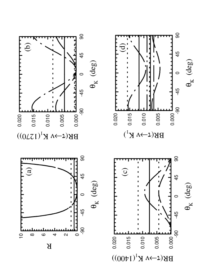
FIG. 1.: The $\tau\to K_{1}\nu$ decay widths as a function of $\theta_{K}$ for the non-relativistic results. $R=BR(\tau\to\nu K_{1}(1270))/BR(\tau\to\nu K_{1}(1400))$. In all figures the dashed curve is for the wavefunctions from Ref. [18] and the dot-dashed curve is for the wavefunctions from Ref. [17]. In the figure for $R$ both curves lie on each other. The solid and dotted lines are for the experimental values and their $1-\sigma$ errors from the TPC/Two-Gamma measurement [4]. In addition, in the figure for $BR(\tau\to\nu K_{1})$, the solid line bounded by the dot-dot-dashed lines are for the CLEO/ALEPH result and their $1-\sigma$ error [19].

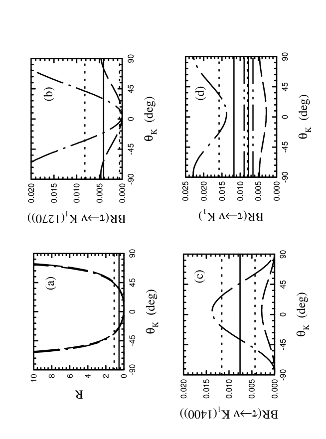
FIG. 2.: The $\tau\to K_{1}\nu$ decay widths as a function of $\theta_{K}$ for the relativized results. The line labelling is the same as in Fig. 1.

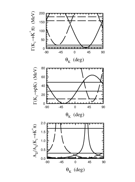
FIG. 3.: Predictions of the pseudoscalar emission model as a function of $\theta_{K}$ for the $K_{1}$ partial widths (to $K^{*}\pi$ and $\rho K$), and ratio of D to S amplitudes (to $K^{*}\pi$). The solid curves are for the $K_{1}(1270)$ and the dashed curves are for the $K_{1}(1400)$. The horizontal lines are the $1-\sigma$ error bounds for the experimental measurements [21] with the same line labelling (solid, dashed) as the predictions. (The experimental lower bound for $K_{1}(1400)\to\rho K$ lies on the axis.)

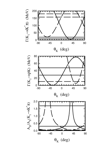
FIG. 4.: Predictions of the ${}^{3}P_{0}$ model as a function of $\theta_{K}$ for the $K_{1}$ partial widths (to $K^{*}\pi$ and $\rho K$), and ratio of D to S amplitudes (to $K^{*}\pi$). The line labelling is the same as in Fig. 3.

TABLE I.: Axial vector decay constants in the nonrelativistic limit using simple harmonic oscillator wavefunctions. The $f_{K_{1}}$ for $|K^{+}\rangle=-|u\bar{s}\rangle$ are given in units of GeV².

Parameter set	$M_{K_{1}}=1.273$ GeV	$M_{K_{1}}=1.402$ GeV
Set 1a	$f_{K_{b}}=-0.049$	$f_{K_{b}}=-0.050$
	$f_{K_{a}}=+0.269$	$f_{K_{a}}=+0.283$
Set 2b	$f_{K_{b}}=-0.070$	$f_{K_{b}}=-0.073$
	$f_{K_{a}}=+0.396$	$f_{K_{a}}=+0.415$

^a From Ref. [18] with $\beta=0.257$ GeV, $m_{u}=m_{d}=0.33$ GeV and $m_{s}=0.55$ GeV.
^b From Ref. [17] with $\beta=0.3$ and $m_{u}=m_{d}$ and $m_{s}$ as above.

TABLE II.: Axial vector decay constants using the relativized mock-meson matrix elements. Simple harmonic oscillator wavefunctions are used with the parameters given below. The $f_{K_{1}}$ for $|K^{+}\rangle=-|u\bar{s}\rangle$are given in units of GeV².

Parameter set	$M_{K_{1}}=1.273$ GeV	$M_{K_{1}}=1.402$ GeV
Set 1a	$f_{K_{b}}=-0.024$	$f_{K_{b}}=-0.025$
	$f_{K_{a}}=+0.220$	$f_{K_{a}}=+0.231$
Set 2b	$f_{K_{b}}=-0.040$	$f_{K_{b}}=-0.042$
	$f_{K_{a}}=+0.486$	$f_{K_{a}}=+0.510$

^a From Ref. [17] with $\beta=0.3$, $m_{u}=m_{d}=0.33$ GeV and $m_{s}=0.55$ GeV.
^b We used effective oscillator parameters from Ref. [6]. They were obtained by fitting simple harmonic oscillator wavefunctions to the rms radii of the wavefunctions of Ref. [6] to obtain $\beta_{K_{1}}=0.45$ GeV. $m_{u}=m_{d}=0.22$ GeV and $m_{s}=0.419$ GeV.

TABLE III.: Strong decay amplitudes for the strange axial mesons using the pseudoscalar emission model, the ${}^{3}P_{0}$ decay model and the flux-tube breaking model. Note that the amplitudes include phase space and are all given in units of MeV^1/2.

Amplitude	Pseudoscalar	${}^{3}P_{0}$	Flux-tube breaking
	emission	Set 1a	Set 1a	Set 2b
$\gamma$		6.25	10.4	12.8
$S(K^{low}_{1}\to\rho K)$	8.02	8.81	8.50	11.0
$D(K^{low}_{1}\to\rho K)$	0.074	0.056	0.057	0.055
$S(K^{low}_{1}\to K^{*}\pi)$	15.5	15.5	14.8	20.5
$D(K^{low}_{1}\to K^{*}\pi)$	2.23	2.36	2.43	2.29
$S(K^{high}_{1}\to\rho K)$	15.4	15.5	14.8	20.1
$D(K^{high}_{1}\to\rho K)$	2.18	2.28	2.34	2.25
$S(K^{high}_{1}\to K^{*}\pi)$	17.3	15.1	14.2	20.7
$D(K^{high}_{1}\to K^{*}\pi)$	4.45	4.61	4.74	4.44
$S(K^{high}_{1}\to K\omega)$	15.1	15.4	14.7	20.0
$D(K^{high}_{1}\to K\omega)$	1.96	2.04	2.10	2.02

^a Simple harmonic oscillator wavefunctions with $\beta=0.40$ GeV, $m_{u}=0.33$ GeV, and $m_{s}=0.55$ GeV.
^b Wavefunctions from Ref. [6].

TABLE IV.: Partial decay widths and ratios of D to S amplitudes of the strange axial mesons for the pseudoscalar emission model, the ${}^{3}P_{0}$ decay model and the flux-tube breaking model using the fitted value of $\theta_{K}$. The widths are given in MeV. $A_{D}/A_{S}$ refers to the ratio of $D$ to $S$ amplitudes. The errors on $\theta_{K}$ are $1-\sigma$.

Decay	Experiment	Pseudoscalar	${}^{3}P_{0}$	Flux-tube breakinga
	(RPP)	emission	Set 1b	Set 1b	Set 2c
$\theta_{K}$		$48^{o}\pm 5^{o}$	$45^{o}\pm 4^{o}$	$44^{o}\pm 4^{o}$	$51^{o}\pm 3^{o}$
$\Gamma(K_{1}(1270)\to\rho K)$	$38\pm 10$	63	75	70	121
$\Gamma(K_{1}(1270)\to K^{*}\pi)$	$14.4\pm 5.5$	16	12	11	35
$|A_{D}/A_{S}(K_{1}(1270)\to K^{*}\pi)|$	$1.0\pm 0.7$	0.64	0.89	1.02	0.40
$\Gamma(K_{1}(1400)\to\rho K)$	$5.2\pm 5.2$	7.9	12	13	6.7
$\Gamma(K_{1}(1400)\to K^{*}\pi)$	$164\pm 16$	286	221	197	400
$\Gamma(K_{1}(1400)\to K\omega)$	$1.7\pm 1.7$	2.3	3.6	3.9	1.9
$|A_{D}/A_{S}(K_{1}(1400)\to K^{*}\pi)|$	$0.04\pm 0.01$	0.058	0.052	0.051	0.062

^a Note that because the flux-tube breaking calculation involves a numerical integral with a 1% error, the two values of $S$ (or $D$) calculated from the $K_{1}(1270)$ and $K_{1}(1400)$ decay results may not agree exactly. In Table III an average value of the two results is given. Because the $S$ and $D$ values in Table III are not exact, using them with Eqn. 43 will not exactly reproduce the flux-tube breaking results show in this table, which are calculated directly from the numerical work.
^b Simple harmonic oscillator wavefunctions with $\beta=0.40$ GeV, $m_{u}=0.33$ GeV, and $m_{s}=0.55$ GeV.
^c Wavefunctions from Ref. [6].