Is $B\to X_{s}\gamma$ equal to $b\to s\gamma$ ?
Spectator contributions to rare inclusive B decays.

Abstract

In $B\to X_{s}\gamma$ there are perturbative $QCD$ corrections at order $\alpha_{s}$ not only to the single quark line process $b\to s\gamma$ but also coming from a set of diagrams where the weak interaction vertex involves a gluon which interacts with the spectator quark in the B hadron. We discuss the impact of the full set of these diagrams. These can influence the decay rate and also the line shape of the photon spectrum as they favor a softer photon energy than does the pure spectator decay $b\to s\gamma$. A subset of these diagrams generate differences in the decay rates for charged and neutral B’s , $B^{+}\to X_{s}\gamma$ vs. $B^{0}\to X_{s}\gamma$ which can be searched for experimentally, although our calculation indicates that the effect will be hard to observe. Bound state effects turn out to be required to give rise to spectator corrections to the decay rate at order $\alpha_{s}$. The resulting contribution to the total rate is rather small (of about $5\%$ ), although the effect is somewhat larger on portions of the photon spectrum.

UMHEP-423

1 Introduction

Rare decays of heavy mesons received considerable interest in the recent years as possible grounds for testing the Standard Model in flavor changing neutral current processes which known to occur only at one loop level [1]. Exclusive decays of $B$-mesons to the non-charmed final states (which are examples of FCNC) are somewhat easier to observe experimentally. However theoretical calculations of exclusive rates include modeling of the hadronization of the final $s(d)$-quark and the resulting predictions vary by the order of magnitude from one to another. The inclusive radiative decay $B\to X_{s}\gamma$ was recently observed by CLEO collaboration [2] and is consistent with the $SM$ expectations. It is now generally accepted that $QCD$ corrections significantly change the decay rate for this process so it is important to bring all of the possible corrections under control to reduce theoretical uncertainties associated with $QCD$.

Most work on the inclusive $B\to X_{s}\gamma$ decay proceeds by calculating radiative corrections to the quark decay $b\to s\gamma$(see for example [3]). However, there are also several diagrams where a radiative correction involves a gluon which interacts with the spectator quark. They generate effects which are not accounted for in spectator model calculations, and the inclusive rate $B\to X_{s}\gamma$ could in principle differ from that of $b\to s\gamma$ at order $\alpha_{s}$. If one is interested in a complete analysis of this decay mode, these non-spectator diagrams must be included. This is especially true if one is interested in the photon spectrum, since reactions which include the spectator quark produce a softer photon spectrum than does the free quark decay. The calculation presented below fills this gap and completes the calculation of the process of inclusive radiative decay of heavy meson at the level $O(\alpha_{s})$

In this paper, we present a $QCD$ based calculation which estimates these non-spectator effects. There are 12 diagrams which we consider, shown in Fig 1. The weak vertices are calculated in $QCD$ perturbation theory (some vertices already exist in the literature), and the ACCMM model [4] is used to calculate the decay rates and spectra. The interference of these diagrams with the leading $b\to s\gamma$ amplitude only occurs for small values of the momentum of the spectator quark. This portion is then particularly sensitive to the bound-state wavefunction, but fortunately the interference is relatively small. The main non-spectator effect comes from the region of phase space where the spectator quark recoils significantly, and hence are second order in $\alpha_{s}$.

The plan of the paper is as follows. In Section 2, we organize the calculation and recall some of the information which in known about the gluonic vertices. Section 3 is devoted to most of the details about the calculation of the modifications to the decay rate and photon spectrum. The impact of the results is described in Section 4. Before proceeding, let us resolve a nomenclature ambiguity. It is conventional to call calculations which focus on the $b\to s\gamma$ transition by the phrase ”spectator model” and to refer to the light quark in the B hadron as the ”spectator” quark. We will continue to use the latter phrase for the light quark in the B meson although, in the diagrams which we consider, it is no longer a spectator but is an active participant in the weak decay. We will call the $b\to s\gamma$ diagrams the spectator process and conversely will label those which actively involve the spectator quark as non-spectator transitions.

2 Diagrams and vertices

There are quite a number of diagrams at order $\alpha_{s}$ which lead to modifications to $B\to X_{s}\gamma$, as shown in Fig 1. Let us divide these into five classes:

1. $QCD$-corrections to the single quark process $b\to s\gamma$.

2. “Gluonic-penguin” (bremstrahlung) diagrams which include $bsg$-vertex with photons emitted from external quark legs.

3. “Triangle” diagrams in which both the gluon and photon are emitted from weak vertex due to a quark loop.

4. Hard gluon spectator exchange diagrams with gluons emitted from $b$ or $s$-lines.

5. Diagram ($10$) involves the $WW\gamma$-vertex and and is suppressed by a power of $1/M_{W}^{2}$. We will not consider this diagram further.

The calculation proceeds by evaluating each of the diagrams, adding them together coherently, integrating over the initial particles momentum using a momentum space wavefunction and summing over the final momenta and spins. The effective vertices are often momentum dependent and depend on the momentum flow in the diagram. Since we are dealing with inclusive decays, the details of hadronization of the final $s$-quark state are not relevant for our discussion (all hadronic final states are summed over), so we have to model only the initial state. This substantially reduces the model-dependence of the final result. However we do have to carefully account for interference effects between the many diagrams, as different diagrams contribute to different portions of the final particles’ phase space. For the $b\to s\gamma$ process, the spectator quark emerges with only low momentum reflecting its momentum in the bound state wavefunction. However in the other diagrams, the final quarks carry a typical momentum of a fraction of the B mass. Interference between the two classes only occurs in a portion of the available phase space. We address this region specifically below. For the initial state wavefunction we use the ACCMM model.

In this calculation we shall encounter two types of vertices: “penguin” and “triangle”.

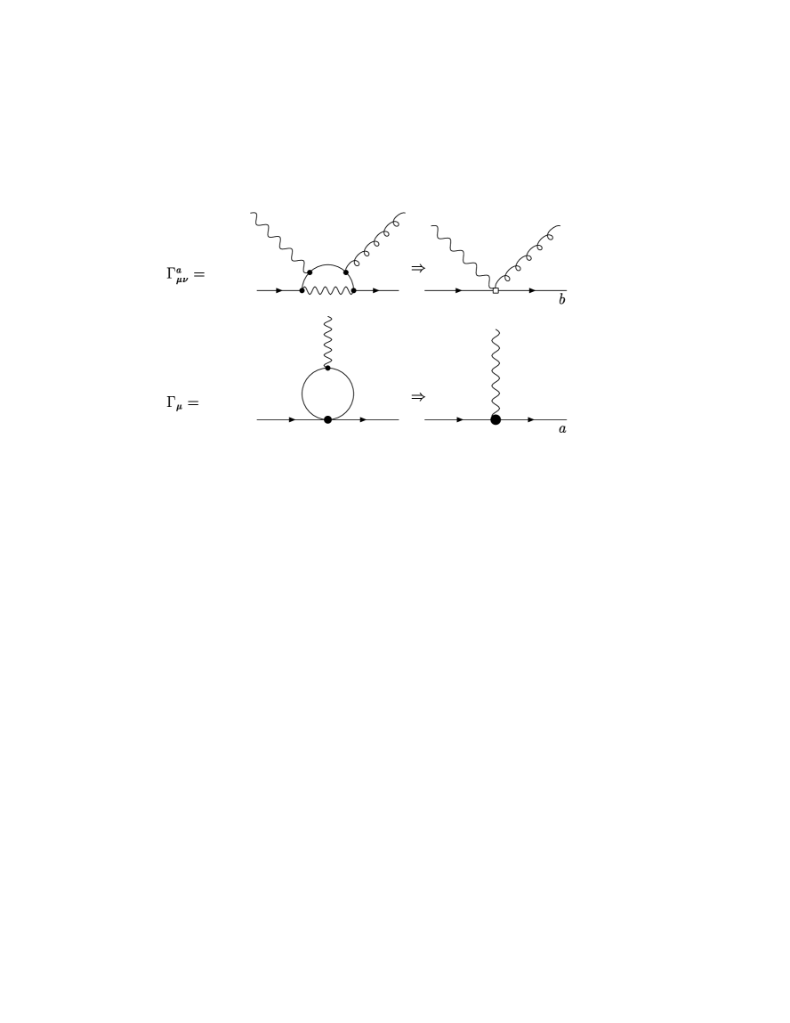
Figure 2: Effective vertices.

1.”Penguin” vertex (Fig.2a). This vertex was calculated quite a while ago [5] and for the $bsg$-interactions turned out to be

$$\Gamma_{\mu}^{a}=-\frac{G_{F}}{\sqrt{2}}V_{bt}V_{ts}\frac{\lambda^{a}}{2}\frac{g_{s}}{8\pi^{2}}\Bigl{(}F_{1}^{g}(x)(k^{2}\gamma_{\mu}-k_{\mu}k\hskip-5.0pt/)(1+\gamma_{5})-m_{b}F_{2}^{g}(x)i\sigma_{\mu\nu}k^{\nu}(1-\gamma_{5})\Bigr{)}$$ (1)

where $x=m_{i}^{2}/m_{W}^{2}$ for $i=c,t$. $F_{1}(x),F_{2}(x)$ are the Inami-Lim functions, $F_{i}^{g}=\sum_{k}F_{ik}^{g}V_{bk}V_{ks}$, using unitarity of CKM matrix we get $F^{g}_{1}=-5.24$ and $F^{g}_{2}=-0.19$ for $m_{t}=176~{}GeV$,$m_{c}=1.3~{}GeV$. Only the magnetic-moment type vertex contributes to the real photon emission in the $b\to s\gamma$, so

$$\Gamma_{\mu}=\frac{G_{F}}{\sqrt{2}}\frac{eQ}{8\pi^{2}}V_{bi}V_{is}m_{b}F_{2}^{\gamma}(x)i\sigma_{\mu\nu}q^{\nu}(1-\gamma_{5})$$ (2)

$F_{2}^{\gamma}(x)\approx 0.65$. We refer to $k$ being the momentum of the gluon and $q$ - momentum of the photon. In the gluon vertex, we shall drop the small contribution from $F_{2}^{g}$, which, however, might be sizable for gluonic penguin-mediated hadronic processes [6].

2. “Triangle” vertex (Fig.2b). The calculation of this vertex reduces to the calculation of the set of usual triangle diagrams with certain form-factors ( a complete parameterization of the diagrams of this type was first given in [7]) and is interesting in the sense that light (spectator quark) current couples to $b\to s$ current through $\epsilon$-tensors. The vertex itself was recently calculated by D.Wyler and H.Simma in [8] and takes the form

$$\Gamma_{\mu\nu}^{a}=-\frac{G_{F}}{\sqrt{2}}\frac{g_{s}eQ}{8\pi^{2}}\frac{\lambda^{a}}{2}V_{bi}V_{is}\Bigl{(}if_{1~{}\mu\nu s}+if_{2~{}\mu\nu s}+if_{3~{}\mu\nu s}\Bigr{)}\gamma^{s}(1+\gamma_{5})$$ (3)

where

$$f_{1~{}\mu\nu s}=\epsilon_{r\mu\nu s}(k^{r}\Delta i_{5}+q^{r}\Delta i_{6})=\epsilon_{r\mu\nu s}l^{r}$$

$$f_{2~{}\mu\nu s}=\frac{\epsilon_{\rho\sigma\mu s}}{kq}k^{\rho}q^{\sigma}k_{\nu}\Delta i_{23}$$ (4)

$$f_{3~{}\mu\nu s}=\frac{\epsilon_{\rho\sigma\nu s}}{kq}k^{\rho}q^{\sigma}q_{\mu}\Delta i_{26}$$

with

$$\Delta i_{5}=-1+\frac{z_{1}}{z_{0}-z_{1}}(Q_{0}(z_{0})-Q_{0}(z_{1}))-\frac{2}{z_{0}-z_{1}}(Q_{-}(z_{0})-Q_{-}(z_{1}))$$

$$\Delta i_{6}=1+\frac{z_{1}}{z_{0}-z_{1}}(Q_{0}(z_{0})-Q_{0}(z_{1}))+\frac{2}{z_{0}-z_{1}}(Q_{-}(z_{0})-Q_{-}(z_{1}))$$

$$\Delta i_{23}=\Delta i_{5}=-\Delta i_{26}$$ (5)

$$Q_{-}(x)=\int_{0}^{1}\frac{du}{u}~{}ln(1-xu(1-u))$$

$$Q_{0}(x)=\int_{0}^{1}du~{}ln(1-xu(1-u))$$

and $z_{0}=s/m_{i}^{2}$,$z_{1}=k^{2}/m_{i}^{2}$, $s$ is a total momentum of internal quarks.

These vertices will be used to calculate the rate and spectrum in the next section. We define the total decay rate as

$$\Gamma_{tot}=\Gamma_{q}+\Gamma_{sc}+\Gamma_{mix}$$ (6)

where $\Gamma_{q}$ represents the leading contributions from $b\to s\gamma$ (diagrams of the class $I$), $\Gamma_{sc}$ gives the corrections which involve the spectator quarks, and $\Gamma_{mix}$ gives the mixing of the two. In powers of the strong coupling constant, $\Gamma_{mix}$ is of order $\alpha_{s}$ and $\Gamma_{sc}$ is of order $\alpha_{s}^{2}$.

In order to account for bound state effects, we will treat the decay of a $B$-meson as a $2\to 3$ scattering process, assuming that the scattering occurs from the bound state and model this state with the ACCMM-model [4]. In calculating the decay rate (cross section $2\to 3$) we average over the spins of the initial particles which, in principle, leads to the prediction for $\Gamma_{tot}$ for the “mixture” of $B$ and $B^{*}$-particles (one can, at the expense of a considerable increase in complexity of the calculation, separate $B$ and $B^{*}$ by introducing polarization operators for projecting out different spin combinations). Thus the decay rate is defined as

$$d\Gamma=\frac{1}{4}~{}\frac{1}{4p_{b}p_{u}}~{}|T_{fi}|^{2}~{}d\Phi$$ (7)

where factor of $4$ in the denominator comes from the spin averaging and

$$d\Phi=(2\pi)^{4}\delta^{4}(p_{f}-p_{i})\frac{d^{3}p_{s}}{(2\pi)^{3}2E_{s}}\frac{d^{3}p_{u}^{\prime}}{(2\pi)^{3}2E_{u}^{\prime}}\frac{d^{3}q}{(2\pi)^{3}2\omega}$$ (8)

We also treat spectator quark as massless to simplify the following calculations. The final phase space integration is performed numerically.

3 Spectator Contributions to the Rate and the Shape of the Photon Spectrum.

3.1 Corrections of order $\alpha_{s}$.

The introduction of interactions with the light quark obviously makes the kinematics of the process more involved - the final state is no longer a simple two-body final state which results in delta-function-like peak in the photon energy distribution. Instead, the peak is now extended down to lower photon energies making it possible for the photon to populate the energy interval from $0$ to $\sim~{}2.5~{}GeV$. Moreover, a difference between the decay spectra of neutral and charged mesons also arises.

The question that naturally appears here is whether it is possible to have an interference of the spectator and non-spectator mechanisms. Since the $b\to s\gamma$ transition is of order $\alpha_{s}^{0}$ and the non-spectator matrix elements are first order in $\alpha_{s}$ this would provide corrections of order $\alpha_{s}$. If there were not any momentum associated with the bound state, the spectator quark would remain precisely at rest in the $b\to s\gamma$ transition and therefore would not interfere with the diagrams where momentum was transferred to the spectator quark. However if bound state effects are present the spectator quark will always carry some momentum (typically of order 1 GeV or less) and the two classes of diagrams can interfere. Since this occurs only over one portion of the phase space, we can say that the interference effects are really of order $\alpha_{s}1GeV/m_{B}$.

In the bound state, the initial momenta are described by a momentum distribution $\phi_{B}(p)$ (which is given by the wave function of quarks inside of the meson).The interference takes place with a probability proportional to a wave-function overlap. We now turn to the calculation of this overlap.

Let $O_{I}$ to be an operator responsible for the transitions via mechanism $I$ and $O_{II}$ - via mechanisms $II-IV$. Then, the mixing term arises as a result of

$$|M_{fi}|^{2}=\sum_{X_{s}}\langle B^{\prime}|O_{I}+O_{II}|X_{s}\rangle\langle X_{s}|O_{I}^{+}+O_{II}^{+}|B\rangle=$$

$$=\langle B^{\prime}|(O_{I}+O_{II})(O_{I}^{+}+O_{II}^{+})|B\rangle=\langle B^{\prime}||O_{I}|^{2}+|O_{II}|^{2}+2Re~{}O_{I}O_{II}^{+}|B\rangle$$ (9)

where we have used completeness relation for $|X_{s}\rangle$-states. We are interested in the last term.

Let us write down the contributions from different classes of diagrams in turn.

$$T_{II}=-\frac{g_{s}e}{8\pi}\frac{1}{k^{2}}\Bigl{\{}\Bigl{(}Q_{b}\Bigl{(}\frac{p_{b}\epsilon}{p_{b}q}-\frac{p_{s}\epsilon}{p_{s}q}\Bigr{)}+Q_{sp}\Bigl{(}\frac{p_{u}\epsilon}{p_{u}q}-\frac{p_{u}^{\prime}\epsilon}{p_{u}^{\prime}q}\Bigr{)}\Bigr{)}\bar{s}(p_{s})\Gamma_{\mu}^{a}b(p_{b})\cdot$$

$$\bar{u}(p_{u}^{\prime})\gamma^{\mu}\lambda_{a}u(p_{u})+\bar{s}(p_{s})\Bigl{(}\Gamma_{\mu}^{a}q\hskip-5.0pt/\frac{\epsilon\hskip-5.0pt/}{2p_{b}q}+\frac{\epsilon\hskip-5.0pt/}{2p_{s}q}q\hskip-5.0pt/\Gamma_{\mu}^{a}\Bigr{)}b(p_{b})~{}\bar{u}(p_{u}^{\prime})\gamma^{\mu}\lambda_{a}u(p_{u})+$$ (10)

$$\bar{s}(p_{s})\Gamma_{\mu}^{a}b(p_{b})~{}\bar{u}(p_{u}^{\prime})\Bigl{(}\gamma^{\mu}\frac{q\hskip-5.0pt/}{2p_{u}q}\epsilon\hskip-5.0pt/+\epsilon\hskip-5.0pt/\frac{q\hskip-5.0pt/}{2p_{u}^{\prime}q}\gamma_{\mu}\Bigl{)}\lambda_{a}u(p_{u})\Bigr{\}}$$

Here $\epsilon$ is the polarization vector of the photon $Q_{b},Q_{sp}$ are the charges of b-quark and spectator respectively, and $\Gamma_{\mu}^{a}$ is given by (1). Note that $k^{2}$ in the denominator due to gluon propagator is to be cancelled by $k^{2}$ in $bsg$-vertex, so $T_{II}$ is a local operator. This operator (convoluted with the lowest order non-spectator graph, along with its charge conjugate part) gives a contribution to the shape of the photon spectrum.

The result of convolution can be represented as

$$T^{2}_{II}=\frac{G_{F}^{2}}{8\pi^{2}}|V_{bt}V_{ts}|^{2}F_{1}^{g}(x)F_{2}^{\gamma}(x)\alpha_{s}(m_{b})\alpha m_{b}C^{1}_{\alpha}$$

$$\Bigl{\{}~{}p_{s}^{\nu}A^{\alpha}q^{\beta}\bar{b}(p_{b})\gamma_{\mu}\gamma_{\nu}\sigma_{\alpha\beta}(1-\gamma_{5})b(p_{b}^{\prime})~{}L^{\mu}+$$

$$+\frac{Q_{b}^{2}}{2p_{s}q~{}p_{b}q}\Bigl{(}S_{b}(q_{\mu}g_{\alpha\nu}-g_{\mu\alpha}q_{\nu})p_{s~{}\theta}-iP_{b}\epsilon_{\mu\alpha t\nu}q_{t}p_{s~{}\theta}\Bigr{)}q^{\beta}~{}$$ (11)

$$\bar{b}(p_{b})\gamma_{\nu}\gamma_{\theta}\sigma_{\alpha\beta}(1-\gamma_{5})b(p_{b}^{\prime})~{}L^{\mu}+\frac{Q_{sp}^{2}}{2p_{u}^{\prime}q~{}p_{u}q}p_{s}^{\nu}q^{\beta}~{}\bar{b}(p_{b})\gamma_{\mu}\gamma_{\nu}\sigma_{\alpha\beta}(1-\gamma_{5})b(p_{b}^{\prime})$$

$$\Bigl{(}S_{u}(q_{\mu}g_{\alpha\theta}-g_{\mu\alpha}q_{\theta})~{}L^{\theta}-iP_{u}\epsilon_{\mu\alpha tu}q_{t}~{}L_{5}^{u}\Bigr{)}\Bigr{\}}+~{}C.c.$$

with $S_{b}=p_{s}q+p_{b}q$, $P_{b}=p_{b}q-p_{s}q$ and analogously for $S_{u}$ and $P_{u}$, $L^{\mu}=\bar{u}(p_{u}^{\prime})\gamma^{\mu}u(p_{u})$, $L_{5}^{\mu}=\bar{u}(p_{u}^{\prime})\gamma^{\mu}\gamma_{5}u(p_{u})$, $C^{1}_{\alpha}=4/3$ is a color factor coming from the averaging over initial colors and summing over the final ones (taking into account the fact that initial and final states are color-singlets). Also

$$A^{\mu}=\frac{p_{b}^{\mu}}{p_{b}q}+\frac{p_{u}^{\mu}}{p_{u}q}-\frac{p_{s}^{\mu}}{p_{s}q}-\frac{{p^{\prime}}_{u}^{\mu}}{p_{u}^{\prime}q},$$

$$\bar{b}(p_{b})\gamma_{\mu}\gamma_{\nu}\sigma_{\alpha\beta}(1-\gamma_{5})b(p_{b}^{\prime})=(g_{\mu\nu}g_{\alpha\beta}+$$

$$g_{\nu\alpha}g_{\mu\beta}-g_{\mu\alpha}g_{\nu\beta}-i\epsilon_{\mu\nu\alpha\beta})\bar{b}(p_{b}^{\prime})(1-\gamma_{5})b(p_{b})-$$ (12)

$$i\bar{b}(p_{b}^{\prime})(g_{\mu\nu}\sigma_{\alpha\beta}+g_{\nu\alpha}\sigma_{\mu\beta}-g_{\mu\alpha}\sigma_{\nu\beta}-i\epsilon_{\mu\nu\alpha\theta}\sigma_{\theta\beta})(1-\gamma_{5})b(p_{b})$$

The calculation of the contribution from the diagrams of the class $III$ is more involved mainly because of the complicated structure of the vertex (3). The amplitude squared reads

$$T_{III}^{2}=\frac{1}{k^{2}}H_{\mu}^{\alpha\beta}L^{\mu}W_{\alpha\beta}=-\frac{Const}{k^{2}}h^{\alpha\alpha}_{\mu}l^{\mu}$$ (13)

with

$$Const=-\frac{G_{F}^{2}}{8\pi^{2}}m_{b}|V_{ts}V_{tb}|^{2}\alpha Q^{2}\alpha_{s}C^{1}_{\alpha}F_{2}^{\gamma}(x)$$

$$l^{\mu}=\bar{u}(p_{u}^{\prime})\gamma^{\mu}u(p_{u})$$ (14)

$$h_{\mu}=2\bar{b}(p^{\prime})\sum_{i}f_{i\mu\alpha s}\sigma_{\alpha\nu}q^{\nu}p\hskip-5.0pt/\gamma^{s}(1+\gamma_{5})b(p)$$

We will be working explicitly with components of this current in order to get $|T_{III}|^{2}$. Using various $\gamma$-matrix identities

$$\sigma_{\alpha\nu}=\frac{i}{2}\Bigl{[}\gamma_{\alpha};\gamma_{\nu}\Bigr{]},$$

$$\gamma_{\alpha}\gamma_{\nu}\gamma_{\theta}=g_{\alpha\nu}\gamma_{\theta}+g_{\nu\theta}\gamma_{\alpha}-g_{\alpha\theta}\gamma_{\nu}-i\epsilon_{\alpha\nu\theta\beta}\gamma_{\beta}\gamma_{5}$$ (15)

we arrive at

$$h^{\mu}=2iq^{\nu}p^{\theta}\bar{b}(p^{\prime})\sum_{i}f^{\mu}_{i\alpha s}\Bigl{\{}g_{\nu\theta}\gamma_{\alpha}\gamma_{s}-g_{\alpha\theta}\gamma_{\nu}\gamma_{s}+i\epsilon_{\alpha\nu\theta\beta}\gamma_{\beta}\gamma_{s}\Bigr{\}}(1+\gamma_{5})b(p)$$ (16)

Note that the term symmetric under $\alpha\leftrightarrow\nu$ disappears. Next, using explicit form of $f_{i\mu\nu s}$, identities

$$\sigma^{\mu\nu}\gamma_{5}=-\frac{i}{2}\epsilon^{\mu\nu\lambda\sigma}\sigma_{\lambda\sigma}$$ (17)

to get rid of $\epsilon$-couplings and discarding terms proportional to $q^{2}$ (on-shell photons), we write

$$h^{\mu}_{\alpha\alpha}=i\bar{b}(p^{\prime})\Bigl{\{}p_{s}^{\mu}((ql)+2\Delta i_{23}(kq))-l^{\mu}(p_{s}q)+q^{\mu}(2(p_{s}l)-4\Delta i_{23}(p_{s}k)+\Delta i_{26}(p_{s}q)+$$

$$+2\Delta i_{23}k^{3}\frac{p_{s}q}{kq})-k^{\mu}(2\Delta i_{23}(p_{s}q))+ik^{\mu}(2\Delta i_{23}\frac{p_{s}q}{kq}\sigma^{\alpha\beta}k_{\alpha}q_{\beta}+\Delta i_{23}\sigma^{\alpha\beta}q_{\alpha}p_{s\beta})$$ (18)

$$+2i(p_{s}q)\sigma^{\mu r}l_{r}-2i(ql)\sigma^{\mu r}p_{s\alpha}+2i(p_{s}l)\sigma^{\mu r}q_{\alpha}-2i\Delta i_{23}(p_{s}k)\sigma^{\mu\alpha}q_{\alpha}+2i\Delta i_{23}((p_{s}q)\sigma^{\mu\alpha}k_{\alpha}$$

$$-\frac{k^{2}}{kq}\sigma^{\mu\alpha}q_{\alpha})-i\Delta i_{23}(kq)\sigma^{\mu\alpha}p_{s\alpha}-\sigma^{\alpha\beta}q_{\alpha}l_{\beta}\sigma^{\mu r}p_{sr}\Bigr{\}}(1+\gamma_{5})b(p)$$

Using (3.1) we obtain the contributions from class $III$. Finally, class $IV$ gives the following

$$T_{IV}=-\frac{i}{k^{2}}\frac{G_{F}}{\sqrt{2}}\frac{eQ}{8\pi^{2}}V_{bi}V_{is}F_{2}^{\gamma}(x)m_{b}g_{s}^{2}\Bigl{\{}\bar{s}(p_{s})\sigma_{\alpha\nu}q^{\nu}(1+\gamma_{5})\lambda_{a}b(p_{b})$$

$$\bar{u}(p_{u})\Bigl{(}\frac{2p\hskip-5.0pt/_{s}}{2p_{s}k+k^{2}}-\frac{2p\hskip-5.0pt/_{b}}{2p_{b}k-k^{2}}\Bigr{)}\lambda_{a}u(p_{u})-\frac{1}{2p_{b}k-k^{2}}\bar{s}(p_{s})\sigma_{\alpha\nu}q^{\nu}(1-\gamma_{5})k\hskip-5.0pt/\gamma_{\mu}\lambda_{a}b(p_{b})$$ (19)

$$\bar{u}(p_{u}^{\prime})\gamma^{\mu}\lambda_{a}u(p_{u})+\frac{1}{2p_{s}k+k^{2}}\bar{s}(p_{s})\gamma_{\mu}k\hskip-5.0pt/\sigma_{\alpha\nu}q^{\nu}(1-\gamma_{5})\lambda_{a}b(p_{b})~{}\bar{u}(p_{u}^{\prime})\gamma^{\mu}\lambda_{a}u(p_{u})\Bigr{\}}$$

Let us also mention that some range of momentum transferred to the spectator gives a contribution to the decay rate which is highly suppressed - in the ACCMM-model, for instance, decay rate looks like

$$\Gamma=\int d^{3}p\phi^{*}_{B}(p^{\prime})\Gamma_{qm}\phi_{B}(p)$$ (20)

with $\vec{p}^{\prime}=\vec{p}+\vec{k}$ and $\phi(p)=(1/p^{3}\sqrt{\pi})exp(-\bar{p}^{2}/2p_{f}^{2})$. Note that this expression reduces to the conventional ACCMM-averaging if the momentum flow between heavy quark and spectator lines is discarded. It is clear that if the magnitude of $3$-momentum transferred to the spectator line is large, the factor of wave function suppression is large as well which results in the exponential fall-off of the $\alpha_{s}$-spectrum as $E_{\gamma}\to 0$. This is the reason why non-spectator $\alpha_{s}$ corrections turn out to give much smaller impact on the line shape of the spectrum than those at order $\alpha_{s}^{2}$, in fact,

$$\frac{\Gamma_{mix}}{\Gamma_{sc}}\leq 1.0\cdot 10^{-2}$$ (21)

3.2 Corrections of order $\alpha_{s}^{2}$.

Let us now consider corrections of order $\alpha_{s}^{2}$. In fact they can simply be obtained by squaring the sum of $T_{i}$ presented in the previous section. We shall present only few of them emphasizing their possible experimental signatures and highlighting some steps of derivations.

Class I. Diagrams of class $I$ give contributions to $\Gamma_{q}$ and have been calculated elsewhere [3]. This contribution to the branching ratio $Br$ varies from $2.0\cdot 10^{-4}$ to $4.2\cdot 10^{-4}$. The major uncertainties at present come from the choice of the renormalization scale in the effective operators and the KM elements, and so this branching ratio can be predicted more accurately in the future as the KM elements are more precisely measured.

Class II. Diagrams of this class give a new contribution to $\Gamma_{tot}$ which comes from the emission of the photon from the spectator quark.

The matrix elements for diagrams ($6$) and ($7$) ( Fig. 1 ) can be rewritten as

$$T_{fi}=\frac{1}{k^{2}}H_{\mu}L_{\alpha}^{\mu}\epsilon^{\alpha}$$ (22)

and are given by (3.1). Taking the hermitian conjugate and multiplying by (3.1) gives $|T_{fi}|^{2}$ for which we can write

$$|T_{fi}|^{2}=\frac{C_{\alpha}^{2}(4\pi)^{2}\alpha_{s}\alpha}{k^{4}}H_{\mu\nu}L^{\mu\nu}_{\alpha\beta}W^{\alpha\beta}$$ (23)

where

$$W^{\alpha\beta}=\sum_{pol}\epsilon^{\alpha*}\epsilon^{\beta}=-g^{\alpha\beta}$$

$$H_{\mu\nu}=Tr\Bigl{\{}p\hskip-5.0pt/_{b}~{}\Gamma_{\mu}^{a}~{}p\hskip-5.0pt/_{s}~{}\Gamma_{\nu}^{b}\Bigr{\}}$$ (24)

$$L_{\alpha\beta}^{\mu\nu ab}=Tr\Bigl{\{}p\hskip-5.0pt/_{u}^{\prime}\Pi^{\mu a}_{\alpha}p\hskip-5.0pt/_{u}\Pi^{\nu a}_{\beta}\Bigr{\}}$$

where as before we set $m_{s}=0$ and $C^{2}_{\alpha}$ is a color factor. To obtain $C^{2}_{\alpha}$ we have used the fact that $B$-meson is a superposition of the color-singlet states, so

$$C^{2}_{\alpha}=\frac{1}{3}tr\Bigl{(}\frac{\lambda_{a}}{2}\frac{\lambda_{b}}{2}\frac{\lambda_{b}}{2}\frac{\lambda_{a}}{2}\Bigr{)}=\frac{16}{9}$$ (25)

Evaluating the traces we obtain for $H_{\mu\nu}$:

$$H_{\mu\nu}=\frac{G_{F}^{2}}{32\pi^{3}}\alpha_{s}|V_{bi}V_{is}|^{2}F_{1}^{g~{}2}k^{4}\Bigl{\{}p_{s\mu}p_{b\nu}+p_{s\nu}p_{b\mu}-(p_{s}p_{b})g_{\mu\nu}+i\epsilon_{\mu\nu\alpha\beta}p_{s}^{\alpha}p_{b}^{\beta}\Bigr{\}}$$ (26)

where the last term vanishes upon contraction with $L_{\alpha\beta}^{\mu\nu}$ for which we can write down (taking into account contraction with $W_{\alpha\beta}$):

$$L_{\alpha\alpha}^{\mu\nu}=Q_{sp}^{2}(2(p_{u}p_{1})(({p_{u}^{\mu}}^{\prime}p_{1}^{\nu})+{p_{u}^{\nu}}^{\prime}p_{u}^{\mu}-g^{\mu\nu}(p_{u}^{\prime}p_{u}))-p_{1}^{2}({p_{u}^{\mu}}^{\prime}p_{u}^{\nu}+{p_{u}^{\nu}}^{\prime}p_{u}^{\mu}-$$

$$g^{\mu\nu}(p_{u}^{\prime}p_{u}))+2p_{2}^{\mu}p_{2}^{\nu}(p_{u}p_{u}^{\prime})+g^{\mu\nu}(2(p_{u}^{\prime}p_{2})(p_{u}p_{2})-p_{2}^{2}(p_{u}p_{u}^{\prime})+$$ (27)

$$p_{2}^{2}(p_{u}^{\mu}{p_{u}^{\nu}}^{\prime}+p_{u}^{\nu}{p_{u}^{\mu}}^{\prime}))-2{p_{u}^{\mu}}^{\prime}p_{2}^{\nu}(p_{u}p_{2})-2p_{u}^{\nu}p_{2}^{\mu}(p_{u}^{\prime}p_{2}))$$

for the diagrams ($6$) and ($7$). These diagrams might be interesting from the experimental point of view since they give rise to different contributions from charged and neutral $B$-mesons (the amplitude is proportional to the charge of spectator $Q_{sp}$), so one, in principle, can observe this charge asymmetry

$$A=\frac{\Gamma(B^{+}\to X_{s}\gamma)-\Gamma(B^{0}\to X_{s}\gamma)}{\Gamma(B^{+}\to X_{s}\gamma)+\Gamma(B^{0}\to X_{s}\gamma)}\sim 0.3\cdot 10^{-3}$$ (28)

However the small size of our prediction means that it will be difficult to make this measurement.

Class III. Calculation of the diagrams of this class involves the effective vertex (3) for the sum of two diagrams - 8 and 9. As before, the amplitude squared can be written in the form

$$|T_{fi}|^{2}=\frac{C_{\alpha}^{2}}{k^{4}}H_{\mu\nu}^{\alpha\beta ab}L^{\mu\nu}_{ab}W^{\alpha\beta}$$

$$H_{\mu\nu ab}^{\alpha\beta}=Tr\Bigl{\{}\Gamma_{\mu}^{\alpha a}~{}p\hskip-5.0pt/_{s}~{}\Gamma_{\nu}^{\beta b}~{}p\hskip-5.0pt/_{b}\Bigr{\}}$$ (29)

$$L^{\mu\nu}=4\Bigl{\{}p_{u}^{\mu}{p_{u}^{n}u}^{\prime}+{p_{u}^{\mu}}^{\prime}p_{u}^{n}u-(p_{u}p_{u}^{\prime})g^{\mu\nu}\Bigr{\}}$$

Expanding $\Gamma_{\mu}^{\alpha a}$ as $\Gamma_{\mu}^{\alpha a}=\sum_{i}f^{a}_{i~{}\mu\alpha s}\gamma_{s}(1+\gamma_{5})$ we get

$$H_{\mu\nu}=\sum_{ik}f_{i\mu\alpha s}f_{k\nu\alpha t}Tr\Bigl{\{}\gamma_{s}(1+\gamma_{5})p\hskip-5.0pt/_{s}\gamma_{t}(1+\gamma_{5})p\hskip-5.0pt/_{b}\Bigr{\}}$$

$$=8\sum_{ik}f_{i\alpha s\mu}f_{k\alpha t\nu}\Bigl{\{}p_{ss}p_{bt}+p_{st}p_{bs}-(p_{s}p_{b})g_{st}+i\epsilon_{stnm}p_{s}^{n}p_{b}^{m}\Bigr{\}}$$ (30)

Thus, the problem is the calculation of $\sum_{ik}f_{i\alpha s\mu}f_{k\alpha t\nu}$. This calculation, which requires the explicit form for the $f$-functions and involves expansions of the products of $\epsilon$-tensors, results in a quite lengthy final expression. However, restricting our attention only to the case of real photons ($q^{2}=0$) and taking advantage of the symmetry of $L^{\mu\nu}$ under $\mu\leftrightarrow\nu$ (implying further convolution with “light” tensor $L^{\mu\nu}$ ) simplify the result enormously since there are only four combinations of $f$’s that give non-vanishing contributions to the problem of interest. They are

$$f_{1~{}\mu s\alpha}f_{1\nu s\beta}=-(l^{2}(g_{\mu\nu}g_{\alpha\beta}-g_{\alpha\nu}g_{\mu\beta})+l_{\mu}l_{\beta}g_{\alpha\nu}+l_{\nu}l_{\alpha}g_{\mu\beta}-l_{\alpha}l_{\beta}g_{\mu\nu}-l_{\mu}l_{\nu}g_{st})$$

$$f_{1~{}\mu s\alpha}f_{2~{}\nu s\beta}+f_{2~{}\mu s\alpha}f_{2~{}\nu s\beta}+f_{2~{}\mu s\alpha}f_{1~{}\nu s\beta}=-\Bigl{(}\frac{{\Delta i_{23}}^{2}}{(kq)^{2}}k^{2}+2\frac{\Delta i_{23}\Delta i_{6}}{kq}\Bigr{)}\epsilon_{\rho\sigma\mu\alpha}\epsilon_{mn\nu\beta}k^{\rho}q^{\sigma}k^{m}q^{n}$$

$$f_{3~{}\mu s\alpha}f_{3~{}\nu s\beta}=-q_{\mu}q_{\nu}\Bigl{(}\frac{\Delta i_{26}}{kq}\Bigr{)}^{2}\Bigl{\{}(kq)(q_{\alpha}k_{\beta}+q_{\beta}k_{\alpha}-(kq)g_{\alpha\beta})-q_{\alpha}q_{\beta}k^{2}\Bigr{\}}$$ (31)

$$f_{3~{}\mu s\alpha}f_{1~{}\nu s\beta}+f_{1~{}\mu s\alpha}f_{3~{}\nu s\beta}=\frac{\Delta i_{26}}{kq}\Bigl{\{}q_{\mu}q_{\nu}(-2(lk)g_{\alpha\beta}+k_{\alpha}l_{\beta}+l_{\alpha}k_{\beta})-q_{\alpha}q_{\nu}(k_{\mu}l_{\beta}-$$

$$(lk)g_{\mu\beta})-q_{\beta}q_{\mu}(k_{\nu}l_{\alpha}-(lk)g_{\alpha\nu})+g_{\alpha\beta}(k_{\mu}q_{\nu}+q_{\mu}k_{\nu})(lq)-(lq)(k_{\alpha}q_{\nu}g_{\mu\beta}+k_{\beta}q_{\mu}g_{\alpha\nu})\Bigr{\}}$$

Combining all of the terms together and contracting $H_{\mu\nu}^{\alpha\alpha}$ to $L^{\mu\nu}$ one obtains the contribution of the class III diagrams to the $\Gamma_{tot}$ which is to be computed numerically. The resulting analytical expression for the amplitude is too long to be presented here.

Class IV. Finally for the class of diagrams responsible for the $b$($s$)-spectator hard gluon exchange, using the same technique as above, we write for $L$ and $H$ tensors

$$L^{\mu\nu}_{ab}=4\Bigl{\{}p_{u}^{\mu}{p^{\prime}}_{u}^{\nu}+{p^{\prime}}_{u}^{\mu}p_{u}^{\nu}-(p_{u}p_{u}^{\prime})g^{\mu\nu}\Bigr{\}}$$

$$H_{\mu\nu ab}^{\alpha\alpha}=Tr\Bigl{\{}p\hskip-5.0pt/_{s}~{}\Pi_{\mu}^{a}~{}p\hskip-5.0pt/_{b}~{}\Pi_{\nu}^{b}\Bigr{\}}$$ (32)

Here the “heavy” current is

$$H^{\alpha a}_{\mu}=\bigl{(}\bar{s}(p_{s})\Gamma^{\alpha}\frac{1}{p\hskip-5.0pt/_{1}-m_{b}}\gamma_{\mu}b(p_{b})+\bar{s}(p_{s})\gamma_{\mu}\frac{1}{p\hskip-5.0pt/_{2}}\Gamma^{\alpha}b(p_{b}))=\bar{s}(p_{s})\Pi^{\alpha a}_{\mu}b(p_{b})$$ (33)

and $\Gamma_{\mu}$ is given by (2). Evaluating the traces and making use of the facts that $L^{\mu\nu}_{ab}$ is symmetric under $\mu\leftrightarrow\nu$ and $q^{2}=0$, we obtain

$$H_{\mu\nu}^{\alpha\alpha}=\frac{G_{F}^{2}}{2\pi}m_{b}^{2}F_{2}^{\gamma~{}2}(x)\alpha\alpha_{s}^{2}Q_{int}^{2}|V_{bi}V_{is}|^{2}C_{\alpha}^{2}\Bigl{[}\frac{32}{k_{1}^{4}(p_{1}^{2}-m_{b}^{2})^{2}}\Bigl{(}(p_{1}^{2}-m_{b}^{2})$$

$$(p_{b}^{\nu}q^{\mu}+p_{b}^{\mu}q^{\nu}-(p_{b}q)g^{\mu\nu})-2(pq)(p_{1}^{\mu}p_{b}^{\nu}+p_{1}^{\nu}p_{b}^{\mu}-(p_{1}p_{b})g^{\mu\nu})\Bigr{)}+$$ (34)

$$\frac{32}{k_{2}^{4}p_{2}^{4}}(p_{b}q)\Bigl{(}p_{2}^{2}(p_{s}^{\mu}q^{\nu}+p_{s}^{\nu}q^{\mu}-(p_{s}q)g^{\mu\nu})-2(p_{2}q)(p_{s}^{\mu}p_{2}^{\nu}+p_{s}^{\nu}p_{2}^{\mu}-(p_{s}p_{2})g^{\mu\nu})\Bigr{)}\Bigr{]}$$

with $p_{1}=p_{s}+q$ and $p_{2}=p_{b}-q$, here $Q_{int}$ is a charge of the internal quarks. Contracting $H_{\mu\nu ab}^{\alpha\alpha}$ with $L^{\mu\nu}_{ab}$ gives the expression for the diagrams of class $IV$. In the final calculation of the magnitude of the spectator effects, the dominant contribution comes from the class $IV$ diagrams [9].

In evaluating the matrix elements, we have taken the $b$-quark spinors to be non-relativistic. The interferences between the different classes of diagrams involving the spectator quark have also been taken into account, although we have not displayed the (lengthy) formulas explicitly above. Some of the complicated sums over many Dirac matrices were evaluated numerically with the help of $Mathematica^{TM}$.

Substituting $|T_{fi}|^{2}$ and (48) into (7), and performing numerical $5$-dimensional Monte-Carlo integration over $\phi_{s},\phi_{q},\theta_{q},\theta_{s},p$ we obtain photon energy distribution presented in Fig.3. Integrating over $x=2\omega/M_{b}$ gives for the decay rate:

$$\delta\Gamma_{tot}\sim 5.3\cdot 10^{-18}~{}GeV$$ (35)

$$\delta Br\sim 1.5\cdot 10^{-5}$$ (36)

Given the recent measured by $CLEO$ value for $Br(B\to X_{s}\gamma)=2.32\cdot 10^{-4}$ [2] we conclude that spectator corrections give an overall effect of about $5\%$ on the inclusive decay rate $\Gamma(B\to X_{s}\gamma)$.

4 Summary

The diagrams which involve the spectator quark are in general non-local and involve momentum transfers to the spectator which are comparable to the energy released in the decay. This is a quite different configuration from the $b\to s\gamma$ transition where the spectator quark is nearly at rest. Despite the inclusion of the bound state momentum of the spectator, the interference of the two classes of diagrams turns out to be very small. We have evaluated the remaining effects of the spectator diagrams, which then amount to effects at order $\alpha_{s}^{2}$.

Our results indicate that the diagrams involving the spectator quark do not play a large role in $B\to X_{s}\gamma$, which implies that the $b\to s\gamma$ reaction is the dominant contribution to the inclusive decay.

Acknowledgments. One of us (A.P.) would like to thank S. Nikolaev for useful conversations regarding Monte-Carlo integration. This work has been supported in part by the US National Science Foundation.

Appendix. Calculation of the Phase Space. Since we are calculating $QCD$-corrections associated with bound-state effects it is convenient to work in the rest frame of $B$-meson. Let us adopt ACCMM-model for use in this particular frame. In this coordinate system (the center of mass frame for the system “heavy quark-spectator”):

$$\vec{p}_{u}^{\prime}+\vec{p}_{s}=0=\vec{p}_{u}+\vec{p}_{b}$$ (37)

$$E_{b}+E_{u}=M_{B}=E_{u}^{\prime}+E_{s}+\omega$$ (38)

We treat the spectator as a massless particle,so

$$E_{u}=p_{u}=p,~{}~{}~{}E_{b}=\sqrt{m_{b}^{2}+p^{2}}$$ (39)

As usual in the ACCMM model the effective $b$ quark mass is momentum dependent and is given by $m_{b}^{2}=M_{B}(M_{B}-2p)$. Also

$$E_{s}=\sqrt{\vec{p}_{s}^{2}}=\sqrt{(\vec{p^{\prime}}_{u}+\vec{q})^{2}}=\sqrt{{E^{\prime}}_{u}^{2}+\omega^{2}+2{E^{\prime}}_{u}\omega cos(\theta^{\prime}_{uq})}$$ (40)

Let us note that in this frame the decay products $u^{\prime},s,q$ lay in the same plane, thus the angle parameters are $\theta^{\prime}_{uq}$-the angle between the directions of $3$-momenta of $s$-quark and photon and the relative angle between $3$-momenta of the initial (“spectator”) $u$-quark and normal to the decay plane. Let us recall that

$$\delta^{4}(p_{f}-p_{i})=\delta(E_{f}-E_{i})\delta^{3}(\vec{p}_{f}-\vec{p}_{i})$$ (41)

Therefore, (8) can be integrated over $\vec{p}_{u}^{\prime}$ to get

$$d\Phi\sim\frac{d^{3}q}{\omega}\frac{d^{3}p^{\prime}_{u}}{E_{u}^{\prime}E_{s}}\delta(M_{B}-E_{u}^{\prime}-E_{s}-\omega)$$ (42)

with $M_{B}^{2}=(E_{b}+E_{u})^{2}$. Next, evaluating the $\vec{p^{\prime}}_{u}$-integral (keeping in mind that $E_{s}$ is given by (40)) yields

$$d\Phi\sim\frac{d^{3}q}{\omega}\frac{d\Omega^{\prime}_{u}{E^{\prime}}_{u}dE^{\prime}_{u}}{E_{s}}\delta(M_{B}-E_{u}^{\prime}-E_{s}-\omega)$$ (43)

Making use of a familiar $\delta$-function relation

$$\delta(f(x))=\sum_{x=x_{0}}\frac{1}{|f^{\prime}(x_{0})|}\delta(x-x_{0})$$ (44)

to perform integration over $E^{\prime}_{u}$ we arrive at the equation for the roots of $E^{\prime}_{u}$:

$$M_{B}-E^{\prime}_{u}-\sqrt{{E^{\prime}}_{u}^{2}+\omega^{2}+2E^{\prime}_{u}\omega cos\theta^{\prime}_{uq}}-\omega=0$$ (45)

which can be solved to get

$$E^{\prime}_{u_{0}}=\frac{M_{B}(M_{B}-2\omega)}{2(M_{B}-\omega(1-cos\theta^{\prime}_{uq}))}.$$ (46)

This gives for the $\delta$-function:

$$\delta(E_{f}-E_{i})=\frac{E_{s}(E^{\prime}_{u_{0}})}{E^{\prime}_{u_{0}}+E_{s}(E^{\prime}_{u_{0}})+\omega cos^{\prime}\theta_{uq}}\delta(E^{\prime}_{u}-E^{\prime}_{u_{0}})$$ (47)

Hence, the phase volume is

$$d\Phi\sim\omega d\omega d\Omega_{q}d\Omega^{\prime}_{u}\frac{M_{B}(M_{B}-2\omega)}{2(M_{B}-\omega(1-cos\theta^{\prime}_{uq}))^{2}}$$ (48)

with $d\Omega_{i}=dcos\theta_{q}d\phi$.

Figure 1: Set of the relevant diagrams.

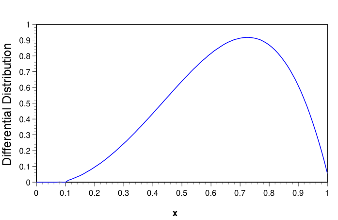
Figure 3: Spectrum for $B\to X_{s}\gamma$.

References

- [1] J. Hewett, SLAC-PUB-95-6782 [hep-ph/9505247] (Talk presented at International Workshop on B Physics, Nagoya, Japan, Oct.1994.)
- [2] CLEO collaboration, CLEO 94-25.
-
[3]
S. Bertolini, F. Borzumati, A. Masiero,
Phys. Rev. Lett. 59 (1987) 180.
M. Misiak, Nucl. Phys. B393 (1993) 23.
B. Grinstein, R. Springer, M.B. Wise, Nucl. Phys. B339 (1990) 269.
A. Ali, C. Greub, Z. Phys. C49 (1990) 431.
A.F. Falk, M. Luke, M.J. Savage, Phys. Rev D49 (1994)3367.
A.J. Buras et. al. Nucl. Phys. B424 (1994) 374.
J.M. Soares, TRI-PP-95-06, hep-ph/9503285. - [4] G. Altarelli et al., Nucl. Phys. B208 (1982)365.
-
[5]
M.A. Shifman, A.I. Vainshtein, V.I. Zakharov,
Phys.Rev. D18 (1978) 2583,
T. Imami, C.S. Lim, Progr. of Theor. Phys. 65 (1981) 297. - [6] N.G. Deshpande, J. Trampetic, Phys.Rev. D41 (1990) 895.
- [7] L. Rosenberg, Phys.Rev. D129 (1963) 2786.
-
[8]
D. Wyler, H.Simma, Nucl.Phys. B344 (1990) 283,
C. Greub, D. Wyler, H. Simma, Nucl. Phys. B434 (1995) 39. -
[9]
C.E. Carlson, J. Milana, hep-ph/9405344,
J. Milana, hep-ph/9503376. -
[10]
R.D. Dikeman, M. Shifman, N.G. Uraltsev,
hep-ph/9505397,
A. Ali, J. Phys. G18 (1992) 1605,
A. Ali, DESY 95-157 [hep-ph/9508335] (review). - [11] A. Ali, T. Ohl, T. Mannel, Phys. Lett. B298 (1993) 195.