Application of HQET to $B\to K^{(*)}$ Transitions

Abstract

We examine the measured rates for the decays $D\to K^{(*)}\ell\nu$, $B\to K^{(*)}\psi^{(\prime)}$ and $B\to K^{*}\gamma$ in a number of scenarios, in the framework of the heavy quark effective theory. We attempt to find a scenario in which all of these decays are described by a single set of form factors. Once such a scenario is found, we make predictions for the rare decays $B\to K^{(*)}\ell^{+}\ell^{-}$. While we find that many scenarios can provide adequate descriptions of all the data, somewhat surprisingly, we observe that two popular choices of form factors, namely monopolar forms and exponential forms, exhibit some shortcomings, especially when confronted with polarization observables. We predict $Br(\bar{B}^{0}\to\bar{K}^{0}\mu^{+}\mu^{-})=6.4\pm 1.0\times 10^{-7}$ and $Br(\bar{B}^{0}\to\bar{K}^{*0}\mu^{+}\mu^{-})=3.8\pm 1.3\times 10^{-6}$. We also make predictions for polarization observables in these decays.

I Introduction

The decays of heavy hadrons have recently received much attention in the literature [1, 2, 3, 4, 5, 6, 7, 8, 9, 10, 11, 12, 13]. From the experimental standpoint, these decays allow access to some of the fundamental parameters of the standard model, such as the elements of the Cabibbo-Kobayashi-Maskawa (CKM) matrix. Questions of CP violation, heavy-flavor oscillations and many others have added to this interest.

From the theoretical standpoint, these processes, and the heavy hadrons themselves, allow various quark models of QCD, as well effective theories, to be tested. In particular, the heavy quark effective theory (HQET) has both been tested by experimental observations, and has played a major role in the extraction of $\left|V_{cb}\right|$ from experimental data [13].

Much of the success of HQET has been in the treatment of decays from one heavy flavor to another, namely $b\to c$ transitions. The effective theory is more limited in scope when applied to heavy-to-light transitions, such as $c\to s$ or $b\to u$. Neverthless, as we will outline in a later section, the scaling behavior of the form factors that describe various weak decays can be deduced [14]. This, in principle, allows the form factors for $b\to s$ transitions to be inferred from those for $c\to s$.

In this article, we assume the validity of the heavy quark symmetry and examine the decays $D\to K^{(*)}\ell\nu$, $B\to K^{(*)}\psi^{(\prime)}$, and the recently measured $B\to K^{*}\gamma$ in a number of scenarios. In particular, we seek a scenario in which all of these decays are adequately described by a single set of form factors. A number of authors have performed similar analyses [15, 16, 17, 18, 19], using the decays $D\to K^{(*)}\ell\nu$ and $B\to K^{(*)}\psi^{(\prime)}$, with varying results.

Once we find a scenario that is satisfactory for the decays mentioned above, we examine, briefly, the decays $B\to K^{(*)}\ell^{+}\ell^{-}$. In this way, we hope to make reliable estimates of the absolute decay rates for these processes. In a later article, we will consider more details of these decays, such as forward-backward asymmetries. These decays, as well as the decay $B\to K^{*}\gamma$, are particularly interesting as the short distance operators responsible arise first at the one-loop-level, and are therefore sensitive to new physics beyond the standard model [20, 21, 22, 23]. However, in order for any effects due to such new physics to be clearly identified, the long distance contributions that arise in the hadronic matrix elements must be well understood. As witness to this, we point out that the inclusive rate $b\to s\gamma$ is reasonably well understood, while the exclusive rate $B\to K^{*}\gamma$ has been predicted to be anywhere from 2% to 40% of this inclusive rate [24].

In the case of the nonleptonic and the rare decays, there arises the crucial issue of the form factors describing the $B\to K^{(*)}$ transition. Such form factors may be estimated in various models, from QCD sum rules, or by applying the scaling relations predicted by HQET to the form factors for the corresponding $D\to K^{(*)}$ transition. The method suggested by HQET, while clearly model-independent, is itself somewhat problematic, as one must take into account the fact that predicting $B\to K^{(*)}\psi$, for instance, requires that these relations be carefully extrapolated beyond the kinematic range accessible in the $D\to K^{(*)}$ transitions. This is because the maximum $q^{2}$ in the $D\to K^{(*)}$ transitions is 1.95 (0.95) GeV², while the $q^{2}$ appropriate to the $B\to K^{(*)}\psi$ transition is 9.6 GeV².

The HQET symmetry predictions relate form factors at the same value of the kinematic variable $v\cdot v^{\prime}$ (or $v\cdot p^{\prime}$), not $q^{2}$, where $v$ and $v^{\prime}$ are the four-velocities of the parent and daughter hadron, respectively. In this case, the extrapolation is from $v\cdot v^{\prime}$ = 2.1 in $D\to K\ell\nu$ to $v\cdot v^{\prime}$ = 3.6 in $B\to K\psi$. The corresponding numbers for the $K^{*}$ decays are 1.3 and 2.0. The question of extrapolation also applies to the rare decays, and is particularly important for the decay $B\to K^{*}\gamma$, for which $q^{2}$ = 0, but $v\cdot v^{\prime}$ = 3.0.

For the nonleptonic decays, a second issue is that of the factorization approximation, which is commonly used to calculate the hadronic matrix elements required. This approximation is not very well founded in general theoretically, yet it appears to work well phenomenologically in the $B$ decays where it has been tested. Nevertheless, application of the form factors of some model or effective theory to the decay $B\to K\psi$, in conjunction with the factorization approximation, serves to probe both issues, and may fail due either to inadequate choice of form factors, failure of the factorization approximation, or both.

The rest of this article is organized as follows. In the next section we describe briefly the effective Hamiltonians and the appropriate hadronic matrix elements for the processes of interest. In section III we use HQET to obtain relations among the form factors of interest. In section IV we discuss our fitting procedure, and present the results for the decays that we are considering. In section V we discuss possible limitations of our results, and suggest questions that may be of interest to both theorists and experimentalists.

II Decay Processes

A Semileptonic Decays

Of the three processes we discuss, the semileptonic decays are perhaps the simplest to treat theoretically. The effective Hamiltonian for these decays is

$${\cal H}_{\rm eff}=\frac{G_{F}}{\sqrt{2}}V_{cs}\bar{s}\gamma_{\mu}\left(1-\gamma_{5}\right)c\bar{\ell}\gamma^{\mu}\left(1-\gamma_{5}\right)\nu_{\ell}.$$ (1)

The hadronic matrix elements for the decays $D\to K^{(*)}\ell\nu$ are

$$\left<K(p^{\prime})\left|\bar{s}\gamma_{\mu}c\right|D(p)\right> = f_{+}(p+p^{\prime})_{\mu}+f_{-}(p-p^{\prime})_{\mu},$$ (2)

$$\left<K(p^{\prime})\left|\bar{s}\gamma_{\mu}\gamma_{5}c\right|D(p)\right> = 0,$$ (3)

$$\left<K^{*}(p^{\prime},\epsilon)\left|\bar{s}\gamma_{\mu}c\right|D(p)\right> = ig\epsilon_{\mu\nu\alpha\beta}\epsilon^{*\nu}(p+p^{\prime})^{\alpha}(p-p^{\prime})^{\beta},$$ (4)

$$\left<K^{*}(p^{\prime},\epsilon)\left|\bar{s}\gamma_{\mu}\gamma_{5}c\right|D(p)\right> = f\epsilon^{*}_{\mu}+a_{+}\epsilon^{*}\cdot p(p+p^{\prime})_{\mu}+a_{-}\epsilon^{*}\cdot p(p-p^{\prime})_{\mu}.$$ (5)

These decays are thus described in terms of six independent, a priori unknown form factors. The terms in $f_{-}$ and $a_{-}$ are unimportant when the lepton mass is ignored, since

$$(p-p^{\prime})_{\mu}\bar{\ell}\gamma^{\mu}(1-\gamma_{5})\nu_{\ell}=(k_{\nu}+k_{\ell})_{\mu}\bar{\ell}\gamma^{\mu}(1-\gamma_{5})\nu_{\ell}=m_{\ell}\bar{\ell}\gamma^{\mu}(1-\gamma_{5})\nu_{\ell}.$$ (6)

In experimental analyses, the form factors $f_{+}$, $a_{+}$, $f$ and $g$ are usually assumed to have the form

$$f_{i}(q^{2})=\frac{f_{i}(0)}{1-\frac{q^{2}}{m_{i}^{2}}},$$ (7)

where $q^{2}=(p-p^{\prime})^{2}$, and $m_{i}$ is a mass, usually taken to be that of the nearest resonance with the appropriate quantum numbers. To date, only the mass appropriate to $f_{+}$ has been measured, and its value measured by CLEO is $2.0\pm 0.22$ GeV [25]. The masses appropriate to $a_{+}$, $f$ and $g$ are assumed to be 2.5 GeV, 2.5 GeV and 2.1 GeV respectively. The $f_{i}(0)$ have the values $0.66\pm 0.03$, $-0.14\pm 0.03$, $0.40\pm 0.07$ and $1.55\pm 0.11$, for $f_{+}$, $a_{+}$, $g$ and $f$, respectively [26].

B Nonleptonic Decays

Neglecting penguin contributions, the effective Hamiltonian for the nonleptonic decays of interest here is

$${\cal H}_{\rm eff} = \frac{G_{F}}{\sqrt{2}}V_{cb}V_{cs}^{*}\left[C_{1}(m_{b})\left(\bar{c}\gamma_{\mu}(1-\gamma_{5})b\right)\left(\bar{s}\gamma^{\mu}(1-\gamma_{5})c\right)\right.$$ (8)

$$+ \left.C_{2}(m_{b})\left(\bar{s}\gamma_{\mu}(1-\gamma_{5})b\right)\left(\bar{c}\gamma^{\mu}(1-\gamma_{5})c\right)\right],$$ (9)

where

$$C_{1}(m_{b}) = \frac{1}{2}\left[\left(\frac{\alpha_{s}(m_{b})}{\alpha_{s}(m_{W})}\right)^{-6/23}+\left(\frac{\alpha_{s}(m_{b})}{\alpha_{s}(m_{W})}\right)^{12/23}\right],$$ (10)

$$C_{2}(m_{b}) = \frac{1}{2}\left[\left(\frac{\alpha_{s}(m_{b})}{\alpha_{s}(m_{W})}\right)^{-6/23}-\left(\frac{\alpha_{s}(m_{b})}{\alpha_{s}(m_{W})}\right)^{12/23}\right].$$ (11)

Here, $m_{W}$ is the mass of the $W$ boson, and $\alpha_{s}(\mu)$ is the running coupling of QCD. This effective Hamiltonian mediates two classes of $B$ nonleptonic decays. The first class contains a $D$ in the final state: $B\to DX$ where $X$ may be $D_{s},D_{s}^{*}$. The second class contains a light meson in the final state: $B\to$ ‘$K$’ $Y$ where $Y$ is now a charmonium state.

To evaluate the matrix elements of the effective Hamiltonian we employ the factorization assumption. By Fierz rearrangement we rewrite the effective Hamiltonian in a form which is suitable for use with this assumption. Both terms of the effective Hamiltonian contribute, in general, but for the decays in which we are interested, only the second term is of interest, and it may be written

$${\cal H}_{\rm eff} = \frac{G_{F}}{\sqrt{2}}V_{cb}V_{cs}^{*}\left(C_{2}(m_{b})+\frac{1}{N_{c}}C_{1}(m_{b})\right)$$ (13)

$$\times\left(\bar{s}\gamma_{\mu}(1-\gamma_{5})b\right)\left(\bar{c}\gamma^{\mu}(1-\gamma_{5})c\right),$$

where $N_{c}$ is the number of colors.

At this point, it has become customary to replace the coupling coefficient by a phenomenological constant $a_{2}$, whose absolute value is measured to be approximately 0.24. The sign of $a_{2}$ is not important for our discussion at this point. It will become important if long distance contributions to the dileptonic rare decays are included.

For the decay $B\to K^{(*)}J/\psi$, we therefore write, after using factorization,

$$\left<J/\psi K^{(*)}\left|\vphantom{K^{(*)}}{\cal H}_{\rm eff}\right|B\right> = \frac{G_{F}}{\sqrt{2}}V_{cb}V_{cs}^{*}a_{2}\left<J/\psi\left|\bar{c}\gamma_{\mu}(1-\gamma_{5})c\right|0\right>$$ (15)

$$\times\left<K^{(*)}\left|\bar{s}\gamma^{\mu}(1-\gamma_{5})b\right|B\right>.$$

The hadronic matrix elements $\left<K^{(*)}\left|\bar{s}\gamma^{\mu}(1-\gamma_{5})b\right|B\right>$ are analogs of those of the previous subsection, so that the form factors required for these matrix elements may, in principle, be obtained from the ‘semileptonic’ decays of $B$ mesons into kaons. Such decays do not take place in the standard model, but we can invoke heavy quark symmetries to relate the form factors needed to those for the semileptonic decays of $D$ mesons to kaons.

The remaining matrix element is

$$\left<J/\psi(p_{\psi},\varepsilon_{\psi})\left|\bar{c}\gamma^{\mu}(1--\gamma_{5})c\right|0\right>=f_{\psi}m_{\psi}\varepsilon_{\psi}^{\mu}.$$ (16)

The decay constant $f_{\psi}$ can be obtained from the leptonic width of the appropriate charmonium vector resonance as

$$f_{\psi}=\sqrt{\Gamma_{\psi\to\ell^{+}\ell^{-}}\frac{27m_{\psi}}{16\alpha^{2}\pi}},$$ (17)

where we have ignored lepton masses. In this way, we find $f_{\psi}$=0.382 GeV, and $f_{\psi^{\prime}}$=0.302 GeV.

C Rare Decays

In the standard model, the effective Hamiltonian for the decay $b\to s\gamma$ is [20, 22, 27]

$${\cal H}_{\rm eff}=-\frac{G_{F}}{\sqrt{2}}\frac{e}{8\pi^{2}}V_{ts}^{*}V_{tb}C_{7}(m_{b})\bar{s}\sigma_{\mu\nu}\left[m_{b}\left(1+\gamma_{5}\right)+m_{s}\left(1-\gamma_{5}\right)\right]bF^{\mu\nu},$$ (18)

where $F^{\mu\nu}$ is the electromagnetic field strength tensor, and the term in $m_{s}$ may be safely ignored. For the decay $b\to s\ell^{+}\ell^{-}$, the corresponding effective Hamiltonian is

$${\cal H}_{\rm eff} = \frac{G_{F}}{\sqrt{2}}\frac{\alpha}{4\pi}V_{ts}^{*}V_{tb}\left[2i\frac{m_{b}}{q^{2}}C_{7}(m_{b})\bar{s}\sigma_{\mu\nu}q^{\nu}(1+\gamma_{5})b\bar{\ell}\gamma^{\mu}\ell\right.$$ (19)

$$+ \left.\vphantom{\frac{4G_{F}}{\sqrt{2}}}C_{9}(m_{b})\bar{s}\gamma_{\mu}\left(1-\gamma_{5}\right)b\bar{\ell}\gamma^{\mu}\ell+C_{10}(m_{b})\bar{s}\gamma_{\mu}\left(1-\gamma_{5}\right)b\bar{\ell}\gamma^{\mu}\gamma_{5}\ell\right].$$ (20)

The Wilson coefficients $C_{i}$ are as in the article by Buras et al. [22]. For the discussion at hand, we have ignored contributions that arise from closed $q\bar{q}$ loops, although these may be easily included.

The only new hadronic matrix elements that arise in the rare decays of interest are

$$\left<K(p^{\prime})\left|\bar{s}\sigma_{\mu\nu}b\right|B(p)\right> = is\left[\left(p+p^{\prime}\right)_{\mu}\left(p-p^{\prime}\right)_{\nu}-\left(p+p^{\prime}\right)_{\nu}\left(p-p^{\prime}\right)_{\mu}\right],$$ (21)

$$\left<K^{*}(p^{\prime},\epsilon)\left|\bar{s}\sigma_{\mu\nu}b\right|B(p)\right> = \epsilon_{\mu\nu\alpha\beta}\left[g_{+}\epsilon^{*\alpha}\left(p+p^{\prime}\right)^{\beta}+g_{-}\epsilon^{*\alpha}\left(p-p^{\prime}\right)^{\beta}\right.$$ (23)

$$\left.+h\epsilon^{*}\cdot p\left(p+p^{\prime}\right)^{\alpha}\left(p-p^{\prime}\right)^{\beta}\right],$$

introducing four new form factors. Due to the relation

$$\sigma^{\mu\nu}\gamma_{5}=\frac{i}{2}\varepsilon^{\mu\nu\alpha\beta}\sigma_{\alpha\beta},$$ (24)

we can easily relate the matrix elements above to those in which the current is $\bar{s}\sigma_{\mu\nu}\gamma_{5}b$. Experimentally, nothing is known about the form factors $s$, $g_{\pm}$ nor $h$.

III HQET And Form Factors

Using the Dirac matrix representation of heavy mesons, one may treat heavy-to-light transitions using the same trace formalism that has been applied to heavy-to-heavy transitions [28, 29]. In the effective theory, a $D$ meson traveling with velocity $v$ is represented as [28, 29]

$$D(v)\to\frac{1+v\hskip-5.0pt/}{2}\gamma_{5}\equiv M_{D}(v),$$ (25)

with an identical representation for a $B$ meson. The meson states of the effective theory are normalized so that

$$\left<{\cal D}(v^{\prime})\left|\right.{\cal D}(v)\right>=2v_{0}\delta^{3}\left({\bf p-p^{\prime}}\right).$$ (26)

The states of QCD and HQET are therefore related by

$$\left|D(v)\right>=\sqrt{m_{D}}\left|{\cal D}(v)\right>.$$ (27)

In all that follows, we will represent the states of full QCD as $\left|D(v)\right>$, and the states of HQET as $\left|{\cal D}(v)\right>$.

Let us consider transitions between such a heavy meson ($D$ meson) and a light meson (kaon) of spin $J$, through a generic flavor changing current. In the effective theory, the matrix element of interest is

$$\left<K^{(J)}(p,\eta)\left|\bar{s}\Gamma h_{v}^{(c)}\right|{\cal D}(v)\right>={\rm Tr}\left\{\Xi\Gamma M_{D}(v)\right\}.$$ (28)

$\Gamma$ is an arbitrary combination of Dirac $\gamma$ matrices, and $\eta$ is the fully symmetric, traceless, transverse, $J$-index tensor that represents the polarization of the state with spin $J$. The matrix $\Xi$ must be the most general that can be constructed from the kinematic variables available, and Dirac $\gamma$ matrices. The most general form for this is [30]

$$\Xi = \eta^{\mu_{1}\dots\mu_{J}}v_{\mu_{1}}\dots v_{\mu_{J-1}}$$ (29)

$$\times \left[v_{\mu_{J}}\left(\xi_{1}^{(J)}(v\cdot p)+p\hskip-5.0pt/\xi_{2}^{(J)}(v\cdot p)\right)+\gamma_{\mu_{J}}\left(\xi_{3}^{(J)}(v\cdot p)+p\hskip-5.0pt/\xi_{4}^{(J)}(v\cdot p)\right)\right]\left(\matrix{1\cr\gamma_{5}}\right).$$ (30)

The $\xi_{i}$’s are uncalculable, nonperturbative functions of the kinematic variable $v\cdot p$, and the 1 ($\gamma_{5}$) is present if the resonance $K^{(J)}$ has natural (unnatural) parity.

From this point on, let us limit the discussion to only two of the kaon resonances, namely the ground-state pseudoscalar kaon itself, and its vector counterpart, $K^{*}$. The above then leads to

$$\left<K(p)\left|\bar{s}\Gamma h_{v}^{(c)}\right|{\cal D}(v)\right> = {\rm Tr}\left\{\left(\xi_{1}+p\hskip-5.0pt/\xi_{2}\right)\gamma_{5}\Gamma M_{D}(v)\right\},$$ (31)

$$\left<K^{*}(p,\epsilon)\left|\bar{s}\Gamma h_{v}^{(c)}\right|{\cal D}(v)\right> = {\rm Tr}\left\{\left[\left(\xi_{3}+p\hskip-5.0pt/\xi_{4}\right)\epsilon^{*}\cdot v+\epsilon\hskip-5.0pt/^{*}\left(\xi_{5}+p\hskip-5.0pt/\xi_{6}\right)\right]\Gamma M_{D}(v)\right\}.$$ (32)

At this point, let us emphasize that the form factors $\xi_{i}$ are independent of the form of $\Gamma$, and so are valid for decays through the left handed current ($\Gamma=\gamma_{\mu}(1-\gamma_{5})$), as well as for rare decays ($\Gamma=\sigma_{\mu\nu}(1\pm\gamma_{5})$). These form factors are also independent of the mass of the heavy quark, and are therefore universal functions. Thus, they are valid for $D\to K$ decays, as well as for $B\to K$ decays. This independence of the quark mass allows us to deduce, in a relatively straightforward manner, the scaling behavior of the usual form factors that describe these transitions [14]. We illustrate this by examining one matrix element in detail.

Consider

$$\left<K(p)\left|\bar{s}\gamma_{\mu}c\right|D(p_{0})\right>=f_{+}(p_{0}+p)_{\mu}+f_{-}(p_{0}-p)_{\mu}$$ (33)

$$= \sqrt{m_{D}}\left<K(p)\left|\bar{s}\gamma_{\mu}h_{v}^{(c)}\right|{\cal D}(v)\right>=\sqrt{m_{D}}{\rm Tr}\left\{\left(\xi_{1}+p\hskip-5.0pt/\xi_{2}\right)\gamma_{5}\gamma_{\mu}\frac{1+v\hskip-5.0pt/}{2}\gamma_{5}\right\},$$ (34)

$$= 2\sqrt{m_{D}}\left(\xi_{1}v_{\mu}-\xi_{2}p_{\mu}\right).$$ (35)

From these equations, one finds that

$$\xi_{1} = \frac{\sqrt{m_{D}}}{2}\left(f_{+}+f_{-}\right),$$ (36)

$$\xi_{2} = \frac{1}{2\sqrt{m_{D}}}\left(f_{-}-f_{+}\right).$$ (37)

Since the $\xi_{i}$ do not scale with the mass of the heavy quark (or meson), it is trivial to deduce that

$$f_{+}+f_{-}\approx m_{D}^{-1/2},\,\,\,\,f_{+}-f_{-}\approx m_{D}^{1/2}.$$ (38)

For the other transitions of interest, the form factors are as defined in the previous section, and the relationships between these and the $\xi_{i}$ are

$$\xi_{1} = \frac{\sqrt{m_{D}}}{2}\left(f_{+}+f_{-}\right),$$ (39)

$$\xi_{2} = \frac{1}{2\sqrt{m_{D}}}\left(f_{-}-f_{+}\right)=-\sqrt{m_{D}}s,$$ (40)

$$\xi_{3} = \frac{m_{D}^{3/2}}{2}\left(a_{+}+a_{-}\right),$$ (41)

$$\xi_{4} = \frac{\sqrt{m_{D}}}{2}\left(2g-a_{+}+a_{-}\right)=m_{D}^{3/2}h,$$ (42)

$$\xi_{5} = -\frac{1}{2\sqrt{m_{D}}}\left(f+2m_{D}v\cdot pg\right)=-\frac{\sqrt{m_{D}}}{2}\left(g_{+}+g_{-}\right),$$ (43)

$$\xi_{6} = \sqrt{m_{D}}g=\frac{1}{2\sqrt{m_{D}}}\left(g_{-}-g_{+}\right).$$ (44)

These expressions yield the additional scaling behavior

$$a_{+}+a_{-}\approx m_{D}^{-3/2},\,\,\,a_{+}-a_{-}\approx m_{D}^{-1/2},$$ (45)

$$f\approx m_{D}^{1/2},\,\,\,g\approx m_{D}^{-1/2},$$ (46)

$$s\approx m_{D}^{-1/2},\,\,\,h\approx m_{D}^{-3/2},$$ (47)

$$g_{+}+g_{-}\approx m_{D}^{-1/2},\,\,\,g_{+}-g_{-}\approx m_{D}^{1/2}.$$ (48)

Eqns. (29) and (31), and consequently eqns. (33-39), contain all of the leading order $m_{D}$ dependence in the form factors, and are valid irrespective of the mass of the strange quark. If the strange quark could be treated as heavy, then we could think of the $\xi_{i}$ as arising from an infinite sum of terms in the $1/m_{s}$ expansion. The leading order forms (in $1/m_{s}$) are also contained in these expressions. These expressions are also valid in the limit of a very light strange quark.

Isgur and Wise [14] have used the scaling of $f_{+}+f_{-}$ ($\approx m_{D}^{-1/2}$) to say that this combination of form factors vanishes (at leading order in $1/m_{D}$), and suggest that one can write $f_{-}=-f_{+}+{\cal O}(1/m_{D})$. Implicit in this argument is the assumption that the strange quark is very light. In our formalism, this amounts to setting $\xi_{1}$ to zero, and we would automatically lose the full scope of our predictions. This is because we could then never recover the limit of a heavy strange quark, for in this limit, $\xi_{1}=-\sqrt{m_{K}}\xi/2$, where $\xi$ is the usual Isgur-Wise function.

The strange quark is such that it may be treated as either heavy or light. We believe that neither the full heavy $s$ limit ($\xi_{1}=-\sqrt{m_{K}}\xi/2$), nor the limit of a very light $s$ quark ($\xi_{1}\to 0$) is completely satisfactory. We assume neither limit in our analysis, and therefore make full use of the predictions of the heavy quark effective theory, which are valid independent of the mass of the strange quark. This means that we retain the form factor $\xi_{1}$ in our discussion and treat it as a completely independent form factor, tying it to neither of the two limits discussed.

At the risk of boring the overly patient reader to tears, and perhaps even to death, we list one more set of relationships among form factors, this time writing the usual form factors in terms of the $\xi_{i}$. The relations are

$$f_{+} = \frac{1}{\sqrt{m_{D}}}\left(\xi_{1}-m_{D}\xi_{2}\right),$$ (49)

$$f_{-} = \frac{1}{\sqrt{m_{D}}}\left(\xi_{1}+m_{D}\xi_{2}\right),$$ (50)

$$f = 2\sqrt{m_{D}}\left(\xi_{5}+v\cdot p\xi_{6}\right),$$ (51)

$$a_{+} = -\frac{1}{m_{D}^{3/2}}\left[\xi_{3}+m_{D}\left(\xi_{6}-\xi_{4}\right)\right],$$ (52)

$$a_{-} = -\frac{1}{m_{D}^{3/2}}\left[\xi_{3}-m_{D}\left(\xi_{6}-\xi_{4}\right)\right],$$ (53)

$$g = \frac{1}{\sqrt{m_{D}}}\xi_{6}.$$ (54)

For the corresponding transitions with a $b$ quark (and a $B$ meson) in the initial state, all factors of $m_{D}$ above must be replaced by $m_{B}$. Using this, rearrangement of eqns. (49) yields

$$f_{+}^{B}(v\cdot p) = \frac{1}{2}\left(\frac{m_{B}}{m_{D}}\right)^{1/2}\left[f_{+}^{D}(v\cdot p)\left(1+\frac{m_{D}}{m_{B}}\right)+f_{-}^{D}(v\cdot p)\left(\frac{m_{D}}{m_{B}}-1\right)\right],$$ (55)

$$f_{-}^{B}(v\cdot p) = \frac{1}{2}\left(\frac{m_{B}}{m_{D}}\right)^{1/2}\left[f_{-}^{D}(v\cdot p)\left(1+\frac{m_{D}}{m_{B}}\right)+f_{+}^{D}(v\cdot p)\left(\frac{m_{D}}{m_{B}}-1\right)\right],$$ (56)

$$f^{B}(v\cdot p) = \left(\frac{m_{B}}{m_{D}}\right)^{1/2}f^{D}(v\cdot p),$$ (57)

$$g^{B}(v\cdot p) = \left(\frac{m_{D}}{m_{B}}\right)^{1/2}g^{D}(v\cdot p),$$ (58)

$$a_{+}^{B}(v\cdot p) = \frac{1}{2}\left(\frac{m_{D}}{m_{B}}\right)^{1/2}\left[a_{+}^{D}(v\cdot p)\left(1+\frac{m_{D}}{m_{B}}\right)+a_{-}^{D}(v\cdot p)\left(\frac{m_{D}}{m_{B}}-1\right)\right],$$ (59)

$$a_{-}^{B}(v\cdot p) = \frac{1}{2}\left(\frac{m_{D}}{m_{B}}\right)^{1/2}\left[a_{-}^{D}(v\cdot p)\left(1+\frac{m_{D}}{m_{B}}\right)+a_{+}^{D}(v\cdot p)\left(\frac{m_{D}}{m_{B}}-1\right)\right],$$ (60)

where $f_{+}^{D}$ is the form factor appropriate to the $D\to K$ transition, while $f_{+}^{B}$ is the form factor appropriate to the $B\to K$ transition, and quantities on the left-hand-sides of eqns. (55) are evaluated at the same values of $v\cdot p$ as those on the right-hand-sides. Omitted from each of eqn. (55) is a QCD scaling factor, discussed below.

Eqns. (55) illustrate two effects, namely the scaling of form factors in going from the $D$ system to the $B$ system, as well as the mixing of $a_{+}$ with $a_{-}$, and $f_{+}$ with $f_{-}$. The effect of this mixing is very important in going from $D$ transitions to $B$ transitions, as it introduces form factors that have not yet been measured experimentally, or to which experiments are not yet sensitive, namely $f_{-}$ and $a_{-}$. In the rates for the semileptonic decays $D\to K^{(*)}\ell\nu$, terms dependent on $f_{-}$ and $a_{-}$ are proportional to the mass of the lepton, and thus play a miniscule role, except near $q^{2}=m_{\ell}^{2}$. Such terms may also be significant if the polarization of the charged lepton is measured.

We close this section with a brief discussion of radiative corrections to the currents and matrix elements that we have discussed. In the limit of a heavy $b$ quark, the full current of QCD is replaced by [31]

$$\bar{s}\Gamma b\to\bar{s}\Gamma h_{v}^{(b)}\left[\frac{\alpha_{s}(m_{b})}{\alpha_{s}(\mu)}\right]^{-\frac{6}{25}}.$$ (61)

This arises from integrating out the $b$ quark, and matching the resulting effective theory onto full QCD at the scale $m_{b}$, at one loop level. At the scale $m_{c}$, we must also integrate out the $c$ quark, but there is also the effect due to running between $m_{b}$ and $m_{c}$. The net effect of this is that the form factors $\xi_{i}$ appropriate to the $b\to s$ transitions are related to those for the $c\to s$ transitions by

$$\xi_{i}^{b\to s}=\xi_{i}^{c\to s}\left[\frac{\alpha_{s}(m_{b})}{\alpha_{s}(m_{c})}\right]^{-\frac{6}{25}}.$$ (62)

The forms of the matrix elements that we discuss above are valid in the limit of infinitely heavy $b$ and $c$ quarks. For quarks of finite mass, there are clearly going to be corrections to the relations we have obtained. In other words, new form factors that appear first at order $1/m_{c}$ and $1/m_{b}$ will begin to make contributions. It is expected that such contributions will become more significant away from the ‘non-recoil’ point, or for $v\cdot p>m_{K^{(*)}}$. This is particularly important for the $B\to K^{(*)}$ decays, as $v\cdot p$ can become very large. Nevertheless, we will apply the relations we have found through all of the available phase space. It is our hope that by doing this, we will at least be able to indicate the suitability of HQET for these transitions. However, since we fit the form factors rather than attempt to calculate them in some model, some of these higher order effects may, in fact, have been included.

IV Results And Discussion

A Data

All of the results we describe are for decays with $\bar{K}^{0}$ (or $\bar{K}^{0*}$) in the final state. The treatment of charged kaons would be identical, and we believe that our results in these channels would be similar in quality to those we obtain for neutral kaons. Before describing the results of our fits, we must comment on how we treat the available data, particularly in the case of the semileptonic decays. Very few of the experimental collaborations have extracted acceptance-corrected distributions [25, 32]. Instead, the form factors are all assumed to be of the monopole form [26], and the parameters are then extracted from the Monte Carlo simulations, with acceptances and efficiencies folded in.

Because of this, we proceed in the inverse sense to generate some ‘simulated data’. We use the published monopole parameters for the form factors to generate $d\Gamma/dq^{2}$ spectra for the semileptonic decays, using the published uncertainties in the monopole parameters to generate uncertainties in the simulated data. In general, these errors are correlated, but we ignore this correlation.

The simulated data generated in this way are completely smooth. We introduce an ‘anti-smoothing’ by smearing the simulated data with a pseudo-randomly generated gaussian distribution of mean zero and standard deviation determined by the errors in the unsmeared simulated data. It is this smeared simulated data that we use for fitting. For the decays $D^{+}\to\bar{K}^{0*}\ell^{+}\nu$, we also include the ratios $\Gamma_{L}/\Gamma$ and $\Gamma_{+}/\Gamma_{-}$ in the fit, where $\Gamma_{\pm}$ are as defined in PDG [26]. In addition, we must point out that the measured decay rates for $D^{+}\to\bar{K}^{0(*)}\ell^{+}\nu$ are somewhat smaller than those for $D^{0}\to\bar{K}^{-(*)}\ell^{+}\nu$, while the published form factor parametrizations are for the average over charge states. To account for this, we rescale the values of the $f_{i}(0)$ to correspond to the smaller rates for neutral kaons. It is these rescaled values that are cited in section II A, and that we use to generate the simulated data.

For the nonleptonic decays, we fit to the PDG averaged decay widths for $\bar{B}^{0}\to\bar{K}^{0}\psi$ and $\bar{B}^{0}\to\bar{K}^{0*}\psi$. In the case of the latter, we also include the ratio $\Gamma_{L}/\Gamma$. For this ratio, we take the averaged value of $0.78\pm 0.073$ as calculated by Gourdin et al. [15, 16]. Masses and lifetimes of mesons are all taken from PDG [26], and we use $V_{tb}=0.9988$, $V_{ts}=0.03$, $V_{cs}=0.9738$, $V_{cb}=0.041$, $m_{b}=4.9$ GeV, $m_{c}$=1.5 GeV, $m_{t}$=177 GeV.

It is worth mentioning that the experimental choice of monopole form factors may be inappropriate, particularly for $f$. In the limit of a heavy strange quark, one finds that $f\propto\left(1+v\cdot v^{\prime}\right)\xi(v\cdot v^{\prime})$, where $\xi$ is the Isgur-Wise function. If $\xi$ is assumed to be monopolar in $q^{2}$, then simple pole dependence for $f$ is inappropriate. Even in the case of a light strange quark, we find that $f\propto\xi_{5}+v\cdot p\xi_{6}$, again indicating that the dependence on the kinematic variable is not simply a monopole form. However, for the range of $q^{2}$ accessible in $D\to K^{*}$ decays, the decay rate is not sensitive to the kinematic dependence. The effect on the decay rate for the nonleptonic and rare decays being considered here, however, are quite significant.

In our fitting, we have separated the decays containing a $K$ meson in the final state from those containing a $K^{*}$ meson in the final state. Thus, for instance, we do not include data on ratios of rates like $\Gamma(D\to K^{*}\ell\nu)/\Gamma(D\to K\ell\nu)$. Our reason is that such ratios introduce correlations between the parameters of the form factors for the two sets of decays.

B Heavy-$s$ Limit

One approximation used recently in the literature has been to treat the strange quark as heavy [33, 34], so that the decays of interest can be treated in the heavy-to-heavy limit. In this limit, the form factors of eqn. (31) may be written

$$\xi_{1} = \xi_{5}=\frac{\sqrt{m_{K}}}{2}\xi,$$ (63)

$$--\xi_{2} = \xi_{6}=\frac{1}{2\sqrt{m_{K}}}\xi,$$ (64)

$$\xi_{3} = \xi_{4}=0,$$ (65)

where $\xi$ is the Isgur-Wise function for heavy-to heavy transitions, and in this limit, $m_{K}=m_{K^{*}}$. In particular, this limit means that $\xi_{5}=m_{K}\xi_{6}$.

We have used this form in fitting the data, and have obtained reasonable fits to the differential decay rates in the semileptonic decays, as well as to the total decay rates in the nonleptonic decays. Polarization ratios, however, are poorly reproduced. In the case of the nonleptonic decay $B\to K^{*}\psi$, the ratio $\Gamma_{L}/\Gamma$ depends only on kinematics, and has a value of 0.43, independent of the form chosen for $\xi$. The experimental value is $0.78\pm 0.07$. In addition, the ratio $\Gamma_{+}/\Gamma_{-}$ in $D\to K^{*}\ell\nu$ always has a value of about 0.4, significantly different from the experimental value of 0.16$\pm$0.04, and largely independent of the form chosen for $\xi$. This indicates that the value of 0.43 obtained for the ratio $\Gamma_{L}/\Gamma$ in $B\to K^{*}\psi$ is not necessarily due to the breakdown of factorization in the heavy $s$ limit, as this limit does not even provide an adequate description of all measurements in the semileptonic decays.

Relaxing the strict heavy-$s$ limit, but constraining the form factors to be near this limit, does not help much, as the polarization observables are still not well reproduced. The conclusion that we draw from this is that the heavy-$s$ limit may give an acceptable description of unpolarized data, but may be dangerous when applied to polarization observables.

C General Features Of Results

All of the results we present are obtained by performing four kinds of fits, namely (1) include the semileptonic decays $D\to K^{(*)}\ell\nu$ only; (1) include the semileptonic decays as well as the nonleptonic decays $B\to K^{(*)}\psi$; (3) include the semileptonic decays, the nonleptonic decays $B\to K^{(*)}\psi$, and the nonleptonic decays $B\to K^{(*)}\psi^{\prime}$; (4) include the measured decay rate for $B\to K^{*}\gamma$ in the fit, as well as the three other decays. Clearly, in the case of the decays to $K$ mesons, we need perform only three kinds of fits. In cases where a measured quantity is not included in the fit, we calculate that quantity using the fit parameters.

We have explored two sets of parametrizations of the form factors. In the first scenario, which we refer to as the exponential scenario, each $\xi_{i}$ has one of the forms

$$\xi_{i} = a_{i}\exp{\left[-b_{i}\left(v\cdot p-m_{K^{(*)}}\right)\right]}=a_{i}\exp{\left[-\frac{b_{i}}{2m_{D}}\left(q^{2}_{{\rm max}}--q^{2}\right)\right]},$$ (66)

$$\xi_{i} = a_{i}\exp{\left[-b_{i}\left(v\cdot p-m_{K^{(*)}}\right)^{2}\right]}=a_{i}\exp{\left[-\frac{b_{i}}{4m_{D}^{2}}\left(q^{2}_{{\rm max}}-q^{2}\right)^{2}\right]},$$ (67)

$$\xi_{i} = a_{i}\exp{\left[-b_{i}\left(v\cdot p\right)^{2}\right]},$$ (68)

while in the second scenario, which we call the multipolar scenario, the forms chosen are

$$\xi_{i}=a_{i}\left(1+b_{i}v\cdot p\right)^{n_{i}},$$ (69)

with $n_{i}=-2,\,-1,\,0,\,1$. In the exponential scenario, eqn. (66) most closely corresponds to the forms that arise in some quark models, most notably that of Isgur and collaborators [35]. However, in such models, the exponential of eqn. (66) is usually multiplied by a polynomial in $v\cdot p$, or equivalently, in $q^{2}$. In the multipolar scenario, $n_{i}=-2$ corresponds to a dipole form factor, while $n_{i}=-1$ represents a monopole. In any one fit, we do not choose all the form factors to have the same form. This means that, for instance, in the case of the decays to $K$ mesons, for which there are two form factors, the second scenario corresponds to sixteen different possible combinations of forms for $\xi_{1}$ and $\xi_{2}$.

In each case, the $a_{i}$ and $b_{i}$ are the free parameters to be varied in the fit. There are therefore twelve free parameters in each fit, to be compared with five extracted and three assumed parameters in the measured semileptonic decays. Since we have more free parameters than are extracted from the experimental data, one might expect that it should be very easy to account for all of the data. In fact, the number of free parameters poses some problems, as it means that the problem is not very well constrained. One consequence of this is that there appear to be several local minima for any particular choice of form factors. Nevertheless, there are some combinations of form factors that simply do not provide adequate descriptions of the data, despite the large number of free parameters.

When only the semileptonic decays are included in the fit, we find that almost any combination of forms for the form factors leads to reasonable results. The few combinations that do not provide good descriptions fail only in their description of the polarization observables.

When we use the exponential forms, we find that we are not able to obtain an adequate description of all of the data simultaneously. In particular, when we include the nonleptonic decays in the fit, the prediction for the rare decay $B\to K^{*}\gamma$ is significantly different from the measured rate. In some cases, however, we find that if we fit the semileptonic decays alone, omitting all of the nonleptonic decays, the prediction for the rare decays is of the right order of magnitude. One possible conclusion here is that factorization is not applicable to these nonleptonic decays, or that there are significant non-factorizable contributions to the amplitude.

In contrast with the exponentials of the first scenario, many combinations of the ‘multipolar’ forms of the second scenario lead to good descriptions of all the data simultaneously. One outstanding feature of all of our results in this scenario (which also exists in the exponential scenario, but to a lesser extent) can be easily understood by examining eqn. (49), where it is seen that $\xi_{6}$ is present in all of the form factors that describe the semileptonic decays $D\to K^{*}$. It is therefore not at all surprising that our results are most sensitive to this form factor. Invariably, we have found that the best fits occur for $\xi_{6}$ linear in $v\cdot p$ (i.e., $n_{6}=1$), independent of the forms chosen for the other form factors. Furthermore, the slope parameter $b_{6}$ is almost always negative, with values lying between -0.4 and -0.65 GeV^-1. The only positive values for $b_{6}$ occur when only the semileptonic decays are included.

The fact that $\xi_{6}$ is so well constrained in our fits means that $f$ and $g$ are also quite well constrained. Since these are the only two form factors that are needed for the decay $B\to K^{*}\gamma$, it is no surprise that we find little variation in the predictions for this decay rate as we vary the parametrizations of $\xi_{3}$, $\xi_{4}$ and $\xi_{5}$, provided that the choice of parametrization of $\xi_{6}$ is unchanged.

For other forms of $\xi_{6}$, we find that at most two of the semileptonic, nonleptonic or rare decays are well accomodated. For instance, if we choose a monopole form for $\xi_{6}$, then in addition to the semileptonic decays, we find that we can accomodate either the nonleptonic decays, the rare decay, but not both. In addition, if we choose all form factors to be monopolar, we fail to find adequate descriptions of the polarization observables, particularly for the ratio $\Gamma_{L}/\Gamma$ measured in the nonleptonic decay.

Our results for the form factors are comparable with those of other authors. Gourdin et al. [15] have found that a number of scenarios, including monopolar form factors, are unable to describe the nonleptonic measurements. Aleksan et al. [17] have found that softening the scaling relations allows an adequate description, while in a second article, Gourdin et al. [16] have found that allowing the form factor $f$ to decrease linearly with $q^{2}$ allows an adequate description of the data. We find that $f$ is quadratic in $q^{2}$, but the absolute value at $q^{2}=0$ for the $B\to K^{*}$ transitions is larger than the absolute value at $q^{2}=q^{2}_{\rm max}$, in keeping with the results of [16], and quite different from pole models.

D Parameters And Form Factors

For each scenario, we have selected a set of fits that we consider to be representative. The parameters for these fits are displayed in table I for the exponential forms, and in table II for the multipolar forms. In the first scenario, the results we have selected correspond to $\xi_{2}$ and $\xi_{3}$ as in eqn. (66), $\xi_{1}$ and $\xi_{4}$ as in eqn. (67), and $\xi_{5}$ and $\xi_{6}$ as in eqn. ( 68). In the second scenario, the $n_{i}$ have the values $n_{i}=(0,-1,1,-2,1,1)$.

TABLE I.: Values of the parameters that result from four different fits, for the exponential scenario. In this table, Fit 1 means that only $D\to K^{(*)}\ell\nu$ is included in the fit; Fit 2 means $D\to K^{(*)}\ell\nu$ and $B\to K^{(*)}J/\psi$ are included; Fit 3 means $D\to K^{(*)}\ell\nu$, $B\to K^{(*)}J/\psi$ and $B\to K^{(*)}\psi^{\prime}$ are included; Fit 4 means $D\to K^{*}\ell\nu$, $B\to K^{*}J/\psi$, $B\to K^{*}\psi^{\prime}$ and $B\to K^{*}\gamma$ are all included, and applies only to decays with $K^{*}$’s in the final state.

Parameter	Fit 1	Fit 2	Fit 3	Fit 4
$a_{1}$	2.497	0.671	0.667	-
$a_{2}$	1.503	-0.265	-0.266	-
$a_{3}$	10.0	8.825	1.745	1.742
$a_{4}$	4.521	5.137	1.259	1.257
$a_{5}$	9.996	9.998	9.990	9.726
$a_{6}$	1.044	1.037	1.080	1.074
$b_{1}$	3.353	1.979	1.984	-
$b_{2}$	4.710	8.0$\times 10^{-5}$	3.1$\times 10^{-6}$	-
$b_{3}$	3.511	0.238	7.6$\times 10^{-5}$	3.0 $\times 10^{-6}$
$b_{4}$	10.0	1.447	1.076	1.076
$b_{5}$	5.914	6.730	6.520	6.458
$b_{6}$	0.585	0.563	0.585	0.581

TABLE II.: Values of the parameters that result from four different fits, for the multipolar scenario. The columns are as in table I.

Parameter	Fit 1	Fit 2	Fit 3	Fit 4
$a_{1}$	3.358	0.144	0.158	-
$a_{2}$	2.929	5.875	5.951	-
$a_{3}$	-10.0	0.162	0.144	0.145
$a_{4}$	-10.0	3.154	2.569	2.365
$a_{5}$	1.399	0.288	0.346	0.451
$a_{6}$	0.055	1.094	1.085	0.922
$b_{1}$	-	-	-	-
$b_{2}$	0.290	10.0	10.0	-
$b_{3}$	-0.507	10.0	10.0	10.0
$b_{4}$	1.134	0.468	0.388	0.354
$b_{5}$	-1.012	-1.042	-1.030	-0.907
$b_{6}$	10.0	-0.439	-0.435	-0.392

To give some sort of meaning to these parameters, we display in tables III and IV, the values of the form factors at $q^{2}=0$, as well as their logarithmic derivatives at the same point. In these tables, the theoretical error that we quote, as well as those that we quote for the rest of our results, are estimates only, and are obtained by using the covariance matrix that results from the fit.

For the monopole form chosen by experimentalists, the logarithmic derivative is

$$\left.\frac{1}{f_{i}(q^{2})}\frac{df_{i}(q^{2})}{dq^{2}}\right|_{q^{2}=0}=\frac{1}{m_{i}^{2}},$$ (70)

where $m_{i}$ is the polar mass. In this way, we can compare our form factors at $q^{2}=0$, and the corresponding slope parameters, with the experimental values. It is gratifying to find that for $f$, $g$ and $f_{+}$, the values we have obtained are, for the most part, quite consistent with the experimental values, for both the exponential and multipolar scenarios. In addition, the logarithmic derivative of $a_{+}$ shows some variation as we go from fit to fit, and there are sizable variations in the values for $f_{-}$, $a_{-}$ and their logarithmic derivatives. These variations are not surprising, as there are no experimental constraints on these quantities. Although the values we obtain for these quantities may lie outside the accepted domain suggested by models, it is nevertheless quite satisfying to note that the values do not change much as we go from Fit 2 to Fit 3 to Fit 4, particularly for the multipolar scenario. It is also interesting that the prefered slope parameter for $a_{+}$ is negative.

TABLE III.: Values of the form factors and their logarithmic derivatives at $q^{2}=0$, for the exponential scenario. The columns are as in table I.

Quantity	Experiment	Fit 1	Fit 2	Fit 3	Fit 4
$f_{+}(0)$	0.66$\pm$0.03	0.59$\pm$0.04	0.66$\pm$0.03	0.66$\pm$0.03	-
$\frac{f^{\prime}_{+}(0)}{f_{+}(0)}$	$0.23\pm 0.09$	0.80$\pm$0.19	0.24$\pm$0.07	0.24$\pm$0.07	-
$f_{-}(0)$	-	0.97$\pm$0.48	-0.06$\pm$0.12	-0.07$\pm$0.12	-
$\frac{f^{\prime}_{-}(0)}{f_{-}(0)}$	-	0.98$\pm$0.17	-2.50$\pm$4.61	- -2.32$\pm$3.96	-
$f(0)$	1.55$\pm$0.11	1.53$\pm$0.10	1.55$\pm$0.07	1.57$\pm$0.11	1.57$\pm$0.08
$\frac{f^{\prime}(0)}{f(0)}$	0.16	0.15$\pm$0.12	0.12$\pm$0.05	0.14$\pm$0.03	0.14$\pm$0.05
$g(0)$	0.40$\pm$0.07	0.35$\pm$0.03	0.36$\pm$0.02	0.37$\pm$0.03	0.37$\pm$0.02
$\frac{g^{\prime}(0)}{g(0)}$	$0.23$	0.36$\pm$0.12	0.35$\pm$0.05	0.36$\pm$0.02	0.36$\pm$0.05
$a_{+}(0)$	-0.14$\pm$0.03	-0.23$\pm$0.05	-0.20$\pm$0.05	-0.19$\pm$0.05	-0.19$\pm$0.04
$\frac{a^{\prime}_{+}(0)}{a_{+}(0)}$	0.16	-3.17$\pm$0.66	-1.72$\pm$0.76	0.03$\pm$0.11	0.03$\pm$0.44
$a_{-}(0)$	-	-2.99$\pm$0.36	-6.33$\pm$1.98	-1.18$\pm$0.05	- -1.18$\pm$0.28
$\frac{a^{\prime}_{-}(0)}{a_{-}(0)}$	-	1.25$\pm$0.15	0.12$\pm$0.08	- -0.05$\pm$0.01	-0.05$\pm$0.11

TABLE IV.: Values of the form factors and their logarithmic derivatives at $q^{2}=0$, for the multipolar scenario. The columns are as in table I.

Quantity	Experiment	Fit 1	Fit 2	Fit 3	Fit 4
$f_{+}(0)$	0.66$\pm$0.03	0.64$\pm$0.06	0.63$\pm$0.02	0.62$\pm$0.04	-
$\frac{f^{\prime}_{+}(0)}{f_{+}(0)}$	$0.23\pm 0.09$	0.29$\pm$0.17	0.29$\pm$0.07	0.29$\pm$0.08	-
$f_{-}(0)$	-	-5.56$\pm$1.88	-0.84$\pm$0.34	-0.86$\pm$0.34	-
$\frac{f^{\prime}_{-}(0)}{f_{-}(0)}$	-	0.03$\pm$0.03	0.21$\pm$0.04	0.21$\pm$0.04	-
$f(0)$	1.55$\pm$0.11	1.55$\pm$0.14	1.55$\pm$0.08	1.53$\pm$0.18	1.54$\pm$0.07
$\frac{f^{\prime}(0)}{f(0)}$	0.16	0.04$\pm$0.12	0.14$\pm$0.06	0.17$\pm$0.20	0.15$\pm$0.05
$g(0)$	0.40$\pm$0.07	0.51$\pm$0.05	0.40$\pm$0.03	0.40$\pm$0.05	0.37$\pm$0.03
$\frac{g^{\prime}(0)}{g(0)}$	$0.23$	0.22$\pm$0.01	0.24$\pm$0.03	0.23$\pm$0.05	0.19$\pm$0.02
$a_{+}(0)$	-0.14$\pm$0.03	-0.24$\pm$0.05	-0.21$\pm$0.04	-0.20$\pm$0.08	-0.20$\pm$0.03
$\frac{a^{\prime}_{+}(0)}{a_{+}(0)}$	0.16	-1.14$\pm$0.33	-1.11$\pm$0.30	-0.93$\pm$0.71	-0.98$\pm$0.27
$a_{-}(0)$	-	3.54$\pm$0.33	-1.37$\pm$0.25	-1.21$\pm$0.61	- -1.21$\pm$0.22
$\frac{a^{\prime}_{-}(0)}{a_{-}(0)}$	-	0.22$\pm$0.02	-0.08$\pm$0.01	- -0.09$\pm$0.11	-0.09$\pm$0.01

The form factors for the $D\to K^{(*)}$ transitions that result from these fits are shown in fig. 1 for the exponential forms, and in fig. 2 for the multipolar forms. In each of these figures, we indicate with arrows the maximum $q^{2}$ possible in the corresponding $D\to K^{(*)}$ decay. The corresponding form factors for the $B\to K^{(*)}$ transitions are shown in figs. 3 and 4 respectively. In these latter figures, the vertical dashed lines indicate the range of $q^{2}$ that correspond to the $D\to K^{(*)}$ decays: the values of $v\cdot p$ within the dashed lines of figs 3 and 4 are the same as those that lie to the left of the arrows in figs. 1 and 2.

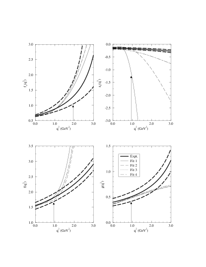
FIG. 1.: Form factors for the $D\to K^{(*)}$ transitions that result from fits, using exponential forms. The thick solid curve is the experimentally extracted form factor, while the thick dashed curves show the range that results from the experimental uncertainties in the parametrizations of the form factors. In each graph, Fit 1 means that only $D\to K^{(*)}\ell\nu$ is included in the fit; Fit 2 means $D\to K^{(*)}\ell\nu$ and $B\to K^{(*)}J/\psi$ are included; Fit 3 means $D\to K^{(*)}\ell\nu$, $B\to K^{(*)}J/\psi$ and $B\to K^{(*)}\psi^{\prime}$ are included; Fit 4 means $D\to K^{*}\ell\nu$, $B\to K^{*}J/\psi$, $B\to K^{*}\psi^{\prime}$ and $B\to K^{*}\gamma$ are all included, and applies only to $a_{+}$, $f$ and $g$. On the scale shown, the curves for Fit 4 are indistinguishable from those of Fit 3. The arrows indicate the maximum $q^{2}$ accessible in the semileptonic decays $D\to K^{(*)}\ell\nu$.

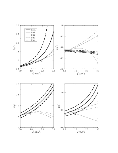
FIG. 2.: Form factors for the $D\to K^{(*)}$ transitions that result from fits, using ‘multipolar’ forms. The key is as in fig. 1.

The effect of the mixing mentioned near the end of the previous section is seen in the curves for $f_{+}^{B}$ and $a_{+}^{B}$. In the case of $f_{+}$ all of the curves for the $D$ form factors are very close to each other, and are all quite similar to the monopole form over the entire range of physically accessible $q^{2}$. Application of eqn. (55), or more truthfully, of eqn. (31), leads to curves for $f_{+}^{B}$ seen in figs. 3 and 4. We point out that the scaling effect due to the coefficient of the $f_{+}^{D}$ term is only about 15%, so that the very different forms for $f_{+}^{B}$ seen in the figures must be attributed to the mixing with $f_{-}^{D}$.

In examining the curves of this figure, one must remember to compare the form factors near the kinematic end points. This means that $f_{+}^{D}$ near $q^{2}=q^{2}_{{\rm max}_{D}}=(m_{D}-m_{K})^{2}=1.95$ GeV² should be compared with $f_{+}^{B}$ near $q^{2}=(m_{B}-m_{K})^{2}=24.8$ GeV². It is very interesting to note that the form factors for the $B\to K^{(*)}$ transitions that result from fitting to the semileptonic decays alone are usually very different from those that result when the nonleptonic decays are included in the fit.

By examining the graphs of figs. 1 and 2, as well as the numbers of tables III and IV, it is clear that the form factors that we have obtained are quite consistent with the experimentally extracted ones, in the range of physically accessible $q^{2}$. Outside of this range, however, all of the form factors we obtain are markedly different from the experimental forms. This clearly has very important consequences for the nonleptonic and rare decays.

FIG. 3.: Form factors for the $B\to K^{(*)}$ transitions that result from fits, using exponential forms. In each graph, Fit 1 means that only $D\to K^{(*)}\ell\nu$ is included in the fit; Fit 2 means $D\to K^{(*)}\ell\nu$ and $B\to K^{(*)}J/\psi$ are included; Fit 3 means $D\to K^{(*)}\ell\nu$, $B\to K^{(*)}J/\psi$ and $B\to K^{(*)}\psi^{\prime}$ are included; Fit 4 means $D\to K^{*}\ell\nu$, $B\to K^{*}J/\psi$, $B\to K^{*}\psi^{\prime}$ and $B\to K^{*}\gamma$ are all included, and applies only to $a_{+}$, $f$ and $g$. The region between the vertical dashed lines is the range of $q^{2}$ for which information is available from the $D\to K^{(*)}\ell\nu$ semileptonic decays.

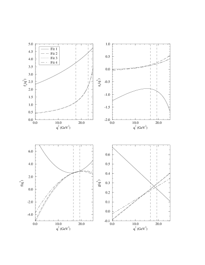
FIG. 4.: Form factors for the $B\to K^{(*)}$ transitions that result from fits, using multipolar forms. The key is as in fig. 3

E Results And Discussion

As can be seen from the numbers in tables V and VI, all fits to the semileptonic decays are reasonable. The quality of the fit with respect to the nonleptonic decays, the results of which are displayed in tables VII and VIII, is quite different, however. In the case of Fit 1, the nonleptonic decays are generally poorly described, while in the case of Fits 2, 3 and 4, the theory does a reasonable job of describing all of the data. The differences between Fits 1 and 2 are shown most graphically in the form factors of figs. 3 and 4. These differences have very significant effects on the decay rates for the rare decays. In general, the differences in the form factors among Fits 2, 3 and 4 are much less striking. We also point out that the striking differences in form factors are achieved, for the most part, with very small adjustments to the intercepts and slope parameters, as seen in tables III and IV.

TABLE V.: Results of fits for semileptonic decays, exponential forms. The columns are as in table I.

Quantity	Experiment	Fit 1	Fit 2	Fit 3	Fit 4
$\Gamma_{D\to K\ell\nu}$ ($10^{-14}$ GeV)	$4.16\pm 0.50$	$4.26\pm 0.28$	$3.91\pm 0.24$	$3.91\pm 0.24$	-
$\Gamma_{D\to K^{*}\ell\nu}$ ($10^{-14}$ GeV)	$2.98\pm 0.25$	$2.88\pm 0.12$	$2.87\pm 0.14$	$2.76\pm 0.12$	$2.77\pm 0.12$
$\frac{\Gamma_{L}}{\Gamma_{T}}\left(D\to K^{*}\ell\nu\right)$	$1.23\pm 0.13$	$1.19\pm 0.12$	$1.23\pm 0.13$	$1.06\pm 0.08$	$1.06\pm 0.10$
$\frac{\Gamma_{+}}{\Gamma_{-}}\left(D\to K^{*}\ell\nu\right)$	$0.16\pm 0.04$	$0.20\pm 0.02$	$0.18\pm 0.02$	$0.18\pm 0.03$	$0.19\pm 0.02$

TABLE VI.: Results of fits for semileptonic decays, multipolar forms. The columns are as in table I.

Quantity	Experiment	Fit 1	Fit 2	Fit 3	Fit 4
$\Gamma_{D\to K\ell\nu}$ ($10^{-14}$ GeV)	$4.16\pm 0.50$	$3.96\pm 0.28$	$3.94\pm 0.23$	$3.95\pm 0.25$	-
$\Gamma_{D\to K^{*}\ell\nu}$ ($10^{-14}$ GeV)	$2.98\pm 0.25$	$2.88\pm 0.12$	$2.87\pm 0.14$	$2.85\pm 0.13$	$2.88\pm 0.10$
$\frac{\Gamma_{L}}{\Gamma_{T}}\left(D\to K^{*}\ell\nu\right)$	$1.23\pm 0.13$	$1.21\pm 0.10$	$1.22\pm 0.09$	$1.20\pm 0.13$	$1.23\pm 0.09$
$\frac{\Gamma_{+}}{\Gamma_{-}}\left(D\to K^{*}\ell\nu\right)$	$0.16\pm 0.04$	$0.16\pm 0.03$	$0.16\pm 0.03$	$0.17\pm 0.04$	$0.20\pm 0.03$

TABLE VII.: Results of fits for nonleptonic decays, exponential forms. The columns are as in table I.

Quantity	Experiment	Fit 1	Fit 2	Fit 3	Fit 4
$\Gamma_{B\to K\psi}$ ($10^{-16}$ GeV)	$3.29\pm 0.95$	$1.27\pm 15.0\times 10^{-4}$	$3.29\pm 0.95$	$3.33\pm 0.95$	-
$\Gamma_{B\to K^{*}\psi}$ ($10^{-16}$ GeV)	$6.93\pm 1.33$	$1.61\pm 1.13$	$7.06\pm 1.48$	$6.75\pm 1.11$	$6.77\pm 1.30$
$\frac{\Gamma_{L}}{\Gamma}\left(B\to K^{*}\psi\right)$	$0.78\pm 0.073$	$0.13\pm 0.21$	$0.77\pm 0.08$	$0.78\pm 0.05$	$0.78\pm 0.07$
$\Gamma_{B\to K\psi^{\prime}}$ ($10^{-16}$ GeV)	$<3.5$	$1.57\pm 10.79\times 10^{-3}$	$1.07\pm 0.25$	$1.08\pm 0.25$	-
$\Gamma_{B\to K^{*}\psi^{\prime}}$ ($10^{-16}$ GeV)	$6.14\pm 3.95$	$22.90\pm 9.10$	$5.75\pm 2.64$	$9.46\pm 0.53$	$9.46\pm 1.18$
$\frac{\Gamma_{L}}{\Gamma}\left(B\to K^{*}\psi^{\prime}\right)$	-	$0.07\pm 0.04$	$0.96\pm 0.02$	$0.76\pm 0.03$	$0.76\pm 0.05$

TABLE VIII.: Results of fits for nonleptonic decays, multipolar forms. The columns are as in table I.

Quantity	Experiment	Fit 1	Fit 2	Fit 3	Fit 4
$\Gamma_{B\to K\psi}$ ($10^{-16}$ GeV)	$3.29\pm 0.95$	$77.02\pm 59.28$	$3.79\pm 0.51$	$3.82\pm 0.65$	-
$\Gamma_{B\to K^{*}\psi}$ ($10^{-16}$ GeV)	$6.93\pm 1.33$	$280.0\pm 52.0$	$6.96\pm 1.30$	$6.86\pm 1.34$	$7.69\pm 1.11$
$\frac{\Gamma_{L}}{\Gamma}\left(B\to K^{*}\psi\right)$	$0.78\pm 0.073$	$0.88\pm 0.03$	$0.78\pm 0.07$	$0.78\pm 0.07$	$0.71\pm 0.05$
$\Gamma_{B\to K\psi^{\prime}}$ ($10^{-16}$ GeV)	$<3.5$	$26.76\pm 17.10$	$1.73\pm 0.33$	$1.75\pm 0.38$	-
$\Gamma_{B\to K^{*}\psi^{\prime}}$ ($10^{-16}$ GeV)	$6.14\pm 3.95$	$26.00\pm 4.50$	$9.11\pm 0.97$	$8.33\pm 2.81$	$8.49\pm 0.80$
$\frac{\Gamma_{L}}{\Gamma}\left(B\to K^{*}\psi^{\prime}\right)$	-	$0.69\pm 0.07$	$0.71\pm 0.05$	$0.70\pm 0.08$	$0.69\pm 0.04$

One comment on the ratio $\rho_{L}=\Gamma_{L}/\Gamma$ in $B\to K^{*}\psi$ is worth making. For many fits, we obtain values for this ratio that are essentially unity. Gourdin et al. [15, 16] state that, assuming factorization of the transition amplitude, this ratio has a maximum value of 0.833. They go on to point out that observation of a value of $\rho_{L}$ greater than this value would be indication of significant non-factorizable contribution to the transition amplitude. In their notation,

$$\rho_{L}=\frac{(a-bx)^{2}}{(a-bx)^{2}+2(1+c^{2}y^{2})},$$ (71)

with $a$, $b$ and $c$ being determined by kinematics, and

$$x=\frac{A_{2}(m_{\psi}^{2})}{A_{1}(m_{\psi}^{2})},\,\,\,\,y=\frac{V(m_{\psi}^{2})}{A_{1}(m_{\psi}^{2})}.$$ (72)

The form factors $A_{1}$, $A_{2}$ and $V$ are those defined by Bauer et al. [36]. The error in their claim arises from ignoring the possibility that $x$ may be large, so that $\rho_{L}\simeq 1$. In our notation, $x\approx(m_{B}-m_{K^{*}})^{2}a_{+}/f$. Thus, we would claim that measurement of $\rho_{L}$ greater than 0.833 is not an indication that factorization is breaking down. Indeed, we have assumed factorization, but in fit 1 of table VIII, we find a value of $\rho_{L}=0.88>0.83$.

In tables IX and X we display our predictions for the rare decays $B\to K^{*}\gamma$, $B\to K\ell^{+}\ell^{-}$ and $B\to K^{*}\ell^{+}\ell^{-}$, obtained using the form factors from the four different fits. The lepton spectra are shown in figs. 5 and 6. As expected, the form factors from Fit 1, especially in the exponential scenario, lead to rates that are ruled out by experimental observations, particularly in the case of the decay $B\to K^{*}\gamma$. In the multipolar scenario, the predictions from Fits 2 and 3 are somewhat larger than the CLEO [24] measurement of $B\to K^{*}\gamma$, while the result from Fit 4 is consistent with the measured value.

TABLE IX.: Predictions for decay rates of rare processes, exponential scenario. The columns are as in table I.

Quantity	Experiment	Fit 1	Fit 2	Fit 3	Fit 4
$\Gamma_{B\to K^{*}\gamma}$ ($10^{-17}$ GeV)	$1.76\pm 0.83$	$0.01\pm 0.03$	$0.02\pm 0.02$	$0.01\pm 0.01$	$0.01\pm 0.01$
$\Gamma_{B\to K\mu^{+}\mu^{-}}$ ($10^{-18}$ GeV)	$<158.0$	$0.30\pm 0.72$	$0.08\pm 0.02$	$0.08\pm 0.02$	-
$\Gamma_{B\to K^{*}\mu^{+}\mu^{-}}^{T}$ ($10^{-18}$ GeV)	-	$0.12\pm 0.05$	$0.13\pm 0.03$	$0.13\pm 0.02$	$0.13\pm 0.02$
$\Gamma_{B\to K^{*}\mu^{+}\mu^{-}}^{L}$ ($10^{-18}$ GeV)	-	$0.13\pm 0.02$	$16.3\pm 12.1$	$1.15\pm 0.20$	$1.15\pm 1.60$
$\Gamma_{B\to K^{*}\mu^{+}\mu^{-}}$ ($10^{-18}$ GeV)	$<10.1$	$0.25\pm 0.06$	$16.5\pm 12.1$	$1.27\pm 0.19$	$1.27\pm 1.60$

TABLE X.: Predictions for decay rates of rare processes, multipolar scenario. The columns are as in table I.

Quantity	Experiment	Fit 1	Fit 2	Fit 3	Fit 4
$\Gamma_{B\to K^{*}\gamma}$ ($10^{-17}$ GeV)	$1.76\pm 0.83$	$77.90\pm 17.80$	$6.17\pm 3.31$	$6.34\pm 4.35$	$2.21\pm 0.72$
$\Gamma_{B\to K\mu^{+}\mu^{-}}$ ($10^{-18}$ GeV)	$<158.0$	$6.33\pm 5.65$	$0.27\pm 0.05$	$0.28\pm 0.05$	-
$\Gamma_{B\to K^{*}\mu^{+}\mu^{-}}^{T}$ ($10^{-18}$ GeV)	-	$5.05\pm 1.04$	$0.33\pm 0.13$	$0.34\pm 0.15$	$0.22\pm 0.03$
$\Gamma_{B\to K^{*}\mu^{+}\mu^{-}}^{L}$ ($10^{-18}$ GeV)	-	$72.7\pm 14.5$	$1.82\pm 1.49$	$1.42\pm 1.25$	$1.45\pm 0.54$
$\Gamma_{B\to K^{*}\mu^{+}\mu^{-}}$ ($10^{-18}$ GeV)	$<10.1$	$77.7\pm 14.4$	$2.15\pm 1.49$	$1.76\pm 1.26$	$1.67\pm 0.55$

Given the failure of the exponential scenario to explain the $B\to K^{*}\gamma$ data, one might be tempted to discard its predictions for the dileptonic decays. However, we see that the integrated rates are, for the most part, quite similar to those predicted in the multipolar scenario. The spectra that result from the two scenarios are very different, however, and the predictions for the relative amount of longitudinally polarized and transversely polarized $K^{*}$ produced are also somewhat different. The exponential forms predict $\Gamma_{T}/\Gamma_{L}\approx 0.1$, while in the multipolar scenario, the ratio ranges between 0.15 and 0.24. The moral here may be that the exponential forms may be adequate for predicting total rates, but not decay spectra, nor polarization observables. We limit our discussion to the multipolar scenario in what follows.

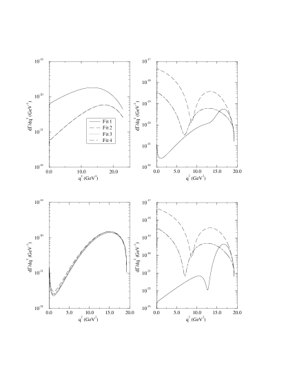
FIG. 5.: Differential decay rates for the processes $B\to K\mu^{+}\mu^{-}$ and $B\to K^{*}\mu^{+}\mu^{-}$, in the exponential scenario. The graphs are, starting at the top left and moving clockwise: $B\to K\mu^{+}\mu^{-}$; $B\to K^{*}\mu^{+}\mu^{-}$; $B\to K^{*}\mu^{+}\mu^{-}$ for longitudinally polarized $K^{*}$’s; $B\to K^{*}\mu^{+}\mu^{-}$ for transversely polarized $K^{*}$’s. In each graph, the key is as in fig. 3.

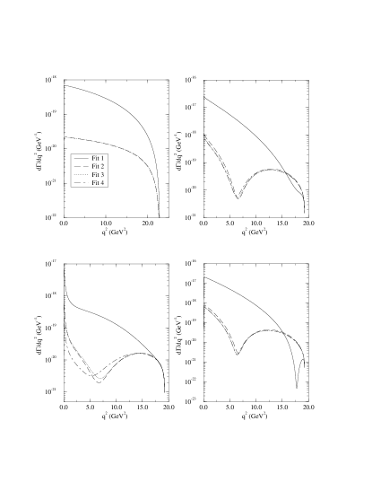
FIG. 6.: Differential decay rates for the processes $B\to K\mu^{+}\mu^{-}$ and $B\to K^{*}\mu^{+}\mu^{-}$, in the multipolar scenario. The graphs are, starting at the top left and moving clockwise: $B\to K\mu^{+}\mu^{-}$; $B\to K^{*}\mu^{+}\mu^{-}$; $B\to K^{*}\mu^{+}\mu^{-}$ for longitudinally polarized $K^{*}$’s; $B\to K^{*}\mu^{+}\mu^{-}$ for transversely polarized $K^{*}$’s. In each graph, the key is as in fig. 3.

The predictions for the process $B\to K\ell^{+}\ell^{-}$ are two to three orders of magnitude smaller than present experimental upper limits, while those for $B\to K^{*}\ell^{+}\ell^{-}$ are smaller than the experimental limits by factors of four to six. We point out, however, that the calculated rates for these last two processes do not include possible contributions from charmonium resonances, which will certainly alter the shape of the lepton spectrum, and should also increase the total decay rate. An investigation of this effect will be left for a future article. However, in at least one experimental analysis, kinematic cuts are imposed on the total mass of the lepton pair, so that events that may arise from either of the first two vector charmonium resonances are excluded [24]. In any case, our results suggest that the exclusive dileptonic decay to the $K^{*}$ should be observed in the near future.

The results that we have obtained here again illustrate that the fit to the present $D\to K^{(*)}$ semileptonic spectra alone is inadequate for providing information on $B\to K^{*}$ processes. Even when we include the nonleptonic decays, the predictions for different decay modes (particularly $B\to K^{*}\ell^{+}\ell^{-}$ with longitudinally polarized $K^{*}$’s) are sensitive to the nonleptonic modes we include in the fit. If any of these predictions are to be taken seriously, we would suggest that most attention be paid to the predictions of Fit 4 in the multipolar scenario, as this is the only scenario that adequately describes all of the data available.

One of the features of the predicted spectra are the minima in the differential decay rates. These minima are the result of zeroes in the respective helicity amplitudes, and the question of whether or not these zeroes do indeed exist, and of their exact locations, will have to await a $B$-factory. However, long-distance effects, such as those that arise from charmonium resonances, or even from the charmonium continuum, will at least alter the positions of the zeroes, and may wash out the effect altogether.

V Conclusion

We have used the scaling predictions of HQET, together with the most recent data on $D\to K^{(*)}\ell\nu$ semileptonic decays, to extract the form factors that describe the $D\to K^{(*)}$ and $B\to K^{(*)}$ processes. The latter we have applied to other processes, namely the nonleptonic decays $B\to K^{(*)}\psi$ and $B\to K^{(*)}\psi^{\prime}$, as well as the rare decays $B\to K^{*}\gamma$ and $B\to K^{(*)}\ell^{+}\ell^{-}$. In the case of the nonleptonic decays, we have assumed factorization of the transition amplitude is valid. We have also performed simultaneous fits of the semileptonic, nonleptonic and rare processes, and have found that HQET, together with factorization, provide an adequate framework for describing the observations. Our predictions for the modes $B\to K^{(*)}\ell^{+}\ell^{-}$ suggest that these should be measurable in the next generation of experiments, and certainly at the proposed $B$ factory.

Perhaps the greatest shortcoming of our fit procedure lies in how we handle the data, or simulated data, for the semileptonic decays. Ideally, we should have attempted to fit our choices of form factors to the experimentally measured differential decay rates. As a second choice, our choices of form factors should have been input into the experimental Monte-Carlo programs to obtain the fit parameters. In any case, it is clear that the present data, particularly in the $D\to K^{*}\ell\nu$ mode, are inadequate to sufficiently constrain the form factors. In addition, the differences in form factors between Fit 1 and Fits 2, 3 and 4 are quite striking.

The scenario that best describes all of the experimental data is the multipolar one, and in this scenario, we find that the universal form factor $\xi_{6}$ is linear in $v\cdot p$. Using this scenario, we predict $Br(\bar{B}^{0}\to\bar{K}^{0}\mu^{+}\mu^{-})=(6.4\pm 1.0)\times 10^{-7}$ and $Br(\bar{B}^{0}\to\bar{K}^{*0}\mu^{+}\mu^{-})=(3.8\pm 1.3)\times 10^{-6}$. These numbers are consistent with other model calculations [24]. We also predict $\Gamma_{T}/\Gamma_{L}$ in $\bar{B}^{0}\to\bar{K}^{*0}\mu^{+}\mu^{-}$ to be $0.15\pm 0.07$.

To fully constrain the predictions of HQET, information on the form factors $a_{-}$ and $f_{-}$ is needed from the semileptonic decays. Such information can only be obtained from high-precision measurements of the decay spectra at low values of $q^{2}$, particularly for semileptonic decays to muons, as well as by measuring the polarization of the charged lepton, again preferably the muon. In addition, the precision and statistics in the $q^{2}$ spectrum must be improved so that the form factor parameters can be extracted from the data, particularly for the decays $D\to K^{*}\ell\nu$. Perhaps the ideal experiment would be the equivalent of present CLEO experiments, in which the machine is tuned to be a source of $B\bar{B}$ pairs, produced from the strong decays of the $\Upsilon(4S)$. For $D$ decays, the equivalent would be to produce a copious number of $\psi(3770)$’s, which can be realized at the proposed tau-charm factory.

- [1] N. Isgur and M. Wise, Phys. Lett. B232 (1989) 113; Phys. Lett. B237 (1990) 527.
- [2] B. Grinstein, Nucl. Phys. B339 (1990) 253.
- [3] H. Georgi, Phys. Lett. B240 (1990) 447.
- [4] A. Falk, H. Georgi, B. Grinstein and M. Wise, Nucl. Phys. B343 (1990) 1.
- [5] A. Falk and B. Grinstein, Phys. Lett. B247 (1990) 406.
- [6] T. Mannel, W. Roberts and Z. Ryzak, Nucl. Phys. B368 (1992) 204.
- [7] M. Luke, Phys. Lett. B252 (1990) 447.
- [8] A. Falk, B. Grinstein and M. Luke, Nucl. Phys. B357 (1991) 185.
- [9] T. Mannel, W. Roberts and Z. Ryzak, Nucl. Phys. B355 (1991) 38.
- [10] N. Isgur and M. B. Wise, Nucl. Phys. B348 (1991) 276.
- [11] H. Georgi, Nucl. Phys. B348 (1991) 293.
- [12] The articles in B Decays, World Scientific (1992), Sheldon Stone, ed., contain many references to the relevant heavy quark literature.
- [13] M. Neubert, Phys. Rep. 245 (1994) 259, and references therein.
- [14] N. Isgur and M. B. Wise, Phys. Rev. D42 (1991) 2388.
- [15] M. Gourdin, A.N. Kamal and X.Y. Pham, Phys. Rev. Lett. 73 (1994) 3355.
- [16] M. Gourdin, Y.Y. Keum and X.Y. Pham, PAR-LPTHE-94-44, unpublished; PAR-LPTHE-95-01, unpublished.
- [17] R. Aleksan, A. Le Yaouanc, L. Oliver, O. Pene and J.C. Raynal, Phys. Rev. D51 (1995) 6235; LPTHE-ORSAY-94-105, unpublished.
- [18] C. Carlson and J. Milana, WM-94-110, unpublished.
- [19] H. - Y. Cheng and B. Tseng, Phys. Rev. D51 (1995) 6259.
- [20] N. G. Deshpande in B Decays, World Scientific (1992), Sheldon Stone, ed.
- [21] D. - S. Liu, UTAS-PHYS-95-08, unpublished; Phys. Lett. B346 (1995) 355.
- [22] A. J. Buras and M. Münz, MPI-PHT-94-96, unpublished.
- [23] G. Burdman, FERMILAB-PUB-95-113-T, unpublished.
- [24] S. Playfer and S. Stone, to appear in International Journal of Modern Physics Letters.
- [25] A. Bean et al., Phys. Lett. B317 (1993) 647.
- [26] L. Montanet et al., Phys. Rev. D50 (1994) 1173.
- [27] W. S. Hou, R. I. Willey and A. Soni, Phys. Rev. Lett. 58 (1987) 1608; B. Grinstein, M. J. Savage and M. B. Wise, Nucl. Phys. B319 (1989) 271; M. Misiak, Nucl. Phys. B393 (1993) 23; M. Misiak, Erratum, Nucl. Phys. B395 (1995) 461; R. Grigjanis, P. J. O’Donnell, M. Sutherland and H. Navelet, Phys. Rep. 228 (1993) 93.
- [28] See for example, H. Georgi, in Proceedings of TASI-91, A. J. Buras and M. Lindner, eds.; B. Grinstein in TASI-94 (1994); W. Roberts, in Physics In Collision 14, S. Keller and H. D. Wahl, eds.
- [29] A. Falk, Nucl. Phys. B378 (1992) 79.
- [30] T. Mannel and W. Roberts, Z. Phys. C61 (1994) 293.
- [31] M. A. Shifman and M. B. Voloshin, Sov. J. Nucl. Phys. 45 (1987) 292; H. D. Politzer and M. B. Wise, Phys. Lett. B206 (1988) 681; H. D. Politzer and M. B. Wise, Phys. Lett. B208 (1988) 504; E. Eichten and B. Hill, Phys. Lett. B234 (1990) 511.
- [32] J. C. Anjos et al., Phys. Rev. Lett. 62 (1989) 1587; ibid, 65 (1990) 2630; K. Kodama et al., Phys. Lett. B274 (1992) 246; Z. Bai et al., Phys. Rev. Lett. 66 (1991) 1011.
- [33] M. R. Ahmady, D. - S. Liu and A. H. Fariborz, HEPPH-9506235, unpublished.
- [34] A. Ali and T. Mannel, Phys. Lett. B264 (1991) 447; Erratum, ibid B274 (1992) 526; A. Ali, T. Ohl and T. Mannel, Phys. Lett. B298 (1993) 195.
- [35] N. Isgur, D. Scora, B. Grinstein and M. B. Wise, Phys. Rev. D39 (1989) 799; D. Scora and N. Isgur, Phys. Rev. D52 (1995) 2783; D. Scora, University of Toronto Ph. D. thesis, unpublished.
- [36] M. Wirbel, B. Stech and M. Bauer, Z. Phys. C29 (1985) 637; M. Bauer, B. Stech and M. Wirbel, Z. Phys. C34 (1987) 103.